Legitimate against Illegitimate IRSs on MISO Wiretap Channels

Abstract

The low-cost legitimate intelligent reflecting surfaces (IRSs) have been applied to the wiretap channel in physical layer security to enhance the secrecy rate. In practice, the eavesdropper can also deploy an IRS, namely illegitimate IRS, to deteriorate the secrecy rate. This paper studies the interplay between a transmitter, a legitimate IRS, and an illegitimate IRS in a multiple-input single-output (MISO) wiretap channel. We formulate a max-min secrecy rate problem, where the channel state and resource allocation information are available at the transmitter as well as the receivers. We aim to design an efficient transmit beamforming and phase shifting strategy of the legitimate IRS, under the worst-case secrecy rate achieved based on optimizing the phase shifting strategy of the illegitimate IRS. We propose three solution methods based on the gradient descent ascent (GDA), the alternate optimization (AO), and the mixed Nash equilibrium (NE) in zero-sum games in strategic form. Numerical results are provided to demonstrate the performance and convergence behavior of AO, GDA, and the mixed NE for continuous and discrete domains of IRSs’ phase shifts.

I Introduction

Intelligent reflecting surface (IRS) has been developed as a key enabler to realize programmable and controllable signal propagation environment [1, 2]. The IRS can be thought of as a low-cost (smart) thin metasurface including passive reflecting elements, each of which is capable of modifying the amplitude and phase of the electromagnetic waves by using external stimuli, resulting in higher spectral efficiency [2, 3]. It has been shown that the passive elements of IRSs lead to much less power consumption compared to the traditional active transceivers or relays [1, 2, 3].

Recent research studies investigate the advantages of IRSs to improve the physical layer security (PLS) of wireless communications [4, 5, 6, 7, 8, 9, 10, 11, 12, 13]. The research studies on IRS-aided wiretap channels mainly focus on the advantages of legitimate IRSs under the control of the transmitter (Alice) to provide secure communications. However, the eavesdropper (Eve) can also use low-cost IRSs, called illegitimate IRSs, to deteriorate the secrecy rate. There are few works on PLS with the existence of illegitimate IRSs. In [14], the authors consider a wiretap channel, where Eve uses an IRS to degrade the legitimate receiver’s (Bob’s) reception by a passive jamming. In [15], a P2P channel with the existence of an IRS jammer is studied. To the best of our knowledge, the interplay between legitimate and illegitimate IRSs on the secrecy rate is not yet studied in the literature. In this work, we consider a new scenario, where both Bob and Eve use independent IRSs under the perfect channel state information. Moreover, the beamforming strategy (Alice’s strategy) as well as the phase shifting strategy of Bob’s IRS (Bob’s strategy) are available at Eve when she is tuning her own IRSs phase shifting elements (Eve’s strategy). Our contributions are as follows:

• We study the impacts of legitimate and illegitimate IRSs on the secrecy rate. In this scenario, we show that depending on some channel conditions, each IRS acts as a signal enhancer for its corresponding receiver or jammer for the other one.

• We design an efficient joint Alice’s (beamforming) and Bob’s (legitimate IRS) strategy to maximize the secrecy rate. To make the algorithm robust, we consider the worst-case secrecy rate achieved by optimizing Eve’s (illegitimate IRS) strategy for any given Alice’s and Bob’s strategies. Hence, we formulate a novel max-min secrecy rate problem.

• We propose three solution methods based on gradient descent ascent (GDA), alternate optimization (AO), and non-cooperative game theory. We numerically evaluate the convergence behavior and performance of AO and GDA for continuous and discrete domains of IRSs’ phase shifting elements.

II System Model and Problem Formulation

II-A System Model

We consider the multiple-input single-output (MISO) wiretap channel, where a single transmitter (Alice) equipped with $M$ antennas communicates with a single-antenna legitimate user (Bob) in the presence of a single-antenna eavesdropper (Eve) overhearing the broadcast signal as shown in Fig. 1. Moreover, an IRS with $N_{\text{B}}$ elements under the control of Alice, namely legitimate IRS or Bob’s IRS, is deployed. Bob’s IRS is responsible for enhancing the data rate of Bob and/or degrading the data rate of Eve, thus enhancing the secrecy rate. Besides, Eve’s IRS with $N_{\text{E}}$ reflecting elements is out of Alice’s control, and is responsible for enhancing Eve’s data rate and/or degrading Bob’s data rate, thus degrading the secrecy rate. The sets of reflecting elements of Bob’s and Eve’s IRS are denoted by $\mathcal{N}_{\text{B}}=\{1,\dots,N_{\text{B}}\}$, and $\mathcal{N}_{\text{E}}=\{1,\dots,N_{\text{E}}\}$, respectively. Theoretically, the reflection coefficient of each IRS element $n$ is modelled by $\alpha_{n}e^{j\beta_{n}}$, where $\alpha_{n}\in[0,1]$ and $\beta_{n}\in[0,2\pi)$ represent the amplitude and phase shift of this element, respectively [16]. We assume the reflecting amplitude $\alpha_{n}=1$ for each reflecting element of Bob’s and Eve’s IRSs, i.e., each reflecting element $n$ can only tune the phase shift $\beta_{n}$. Thus the reflecting element is referred to as phase shifting element.

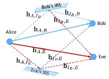
Figure 1: The exemplary model of an IRS-assisted MISO wiretap channel with the existence of an illegitimate IRS.

Let $\boldsymbol{\theta}_{\text{B}}=\left[\theta^{\text{B}}_{1},\dots,\theta^{\text{B}}_{N_{\text{B}}}\right]^{T}$ and $\boldsymbol{\theta}_{\text{E}}=\left[\theta^{\text{E}}_{1},\dots,\theta^{\text{E}}_{N_{\text{E}}}\right]^{T}$ denote the vectors of phase shifting coefficients of Bob’s and Eve’s IRS, respectively, where $\theta^{\text{B}}_{m}=e^{j\phi^{\text{B}}_{m}},~{}\forall m\in\mathcal{N}_{\text{B}}$, and $\theta^{\text{E}}_{n}=e^{j\phi^{\text{E}}_{n}},~{}\forall n\in\mathcal{N}_{\text{E}}$. The parameters $\phi^{\text{B}}_{m}\in[0,2\pi)$ and $\phi^{\text{E}}_{n}\in[0,2\pi)$ represent the phases of the $m$-th and $n$-th phase shifting elements of Bob’s and Eve’s IRS, respectively. In practice, due to the hardware limitation, the phase shifts can take only a finite number of discrete values [17]. Denoted by $L_{\text{B}}$ and $L_{\text{E}}$, the number of discrete values that each phase shifting element of Bob’s and Eve’s IRS can take, respectively. Without loss of generality, we assume that $\phi^{\text{B}}_{m}\in\{\frac{2k\pi}{L_{\text{B}}}|k=0,\dots,(L_{\text{B}}-1)\},~{}\forall m\in\mathcal{N}_{\text{B}}$, and $\phi^{\text{E}}_{n}\in\{\frac{2k\pi}{L_{\text{E}}}|k=0,\dots,(L_{\text{E}}-1)\},~{}\forall n\in\mathcal{N}_{\text{E}}$, [11, 3]. Subsequently, we define the discrete set of possible phase shifting coefficients of each phase shifting element of Bob’s and Eve’s IRS, respectively, by $\mathcal{L}_{\text{B}}=\{e^{j\frac{2k\pi}{L_{\text{B}}}}|k=0,\dots,(L_{\text{B}}-1)\}$, and $\mathcal{L}_{\text{E}}=\{e^{j\frac{2k\pi}{L_{\text{E}}}}|k=0,\dots,(L_{\text{E}}-1)\}$.

In this system, Alice intends to send a confidential message by the independent and identically distributed Gaussian code symbol $x\in\mathbb{C}$ with zero mean and unit variance to Bob over a quasi-static flat-fading Gaussian wiretap channel. The beamforming vector is denoted by $\mathbf{w}\in\mathbb{C}^{M\times 1}$. The generally complex channel vector/matrix from Alice to Bob, Alice to Bob’s IRS, Bob’s IRS to Bob, Bob’s IRS to Eve, Alice to Eve, Alice to Eve’s IRS, Eve’s IRS to Eve, and Eve’s IRS to Bob are denoted by $\mathbf{h}_{\text{A,B}}\in\mathbb{C}^{1\times M}$, $\mathbf{h}_{\text{A,$\text{I}_{\text{B}}$}}\in\mathbb{C}^{N_{\text{B}}\times M}$, $\mathbf{h}_{\text{$\text{I}_{\text{B}}$,B}}\in\mathbb{C}^{1\times N_{\text{B}}}$, $\mathbf{h}_{\text{$\text{I}_{\text{B}}$,E}}\in\mathbb{C}^{1\times N_{\text{B}}}$, $\mathbf{h}_{\text{A,E}}\in\mathbb{C}^{1\times M}$, $\mathbf{h}_{\text{A,$\text{I}_{\text{E}}$}}\in\mathbb{C}^{N_{\text{E}}\times M}$, $\mathbf{h}_{\text{$\text{I}_{\text{E}}$,E}}\in\mathbb{C}^{1\times N_{\text{E}}}$, $\mathbf{h}_{\text{$\text{I}_{\text{E}}$,B}}\in\mathbb{C}^{1\times N_{\text{E}}}$, respectively. We assume that the perfect CSI of all the links is available at all the nodes. The received signal at Bob and Eve can thus be formulated, respectively by

$$y_{B} =\underbrace{\left(\mathbf{h}_{\text{A,B}}+\mathbf{h}_{\text{$\text{I}_{\text{B}}$,B}}\mathbf{\Theta}_{\text{B}}\mathbf{h}_{\text{A,$\text{I}_{\text{B}}$}}+\mathbf{h}_{\text{$\text{I}_{\text{E}}$,B}}\mathbf{\Theta}_{\text{E}}\mathbf{h}_{\text{A,$\text{I}_{\text{E}}$}}\right)}_{\mathbf{h}_{\text{B}}\left(\mathbf{\Theta}_{\text{B}},\mathbf{\Theta}_{\text{E}}\right)}\mathbf{w}x+n_{B},$$ (1)

$$y_{E} =\underbrace{\left(\mathbf{h}_{\text{A,E}}+\mathbf{h}_{\text{$\text{I}_{\text{E}}$,E}}\mathbf{\Theta}_{\text{E}}\mathbf{h}_{\text{A,$\text{I}_{\text{E}}$}}+\mathbf{h}_{\text{$\text{I}_{\text{B}}$,E}}\mathbf{\Theta}_{\text{B}}\mathbf{h}_{\text{A,$\text{I}_{\text{B}}$}}\right)}_{\mathbf{h}_{\text{E}}\left(\mathbf{\Theta}_{\text{B}},\mathbf{\Theta}_{\text{E}}\right)}\mathbf{w}x+n_{E},$$ (2)

in which $\mathbf{\Theta}_{\text{B}}=\text{diag}\left(\boldsymbol{\theta}_{\text{B}}\right)$, $\mathbf{\Theta}_{\text{E}}=\text{diag}\left(\boldsymbol{\theta}_{\text{E}}\right)$, and $n_{B}$ and $n_{E}$ are the independent zero-mean additive white Gaussian noises (AWGNs) at Bob and Eve with variances $\sigma^{2}_{B}$ and $\sigma^{2}_{E}$, respectively. The row vectors $\mathbf{h}_{\text{B}}\left(\mathbf{\Theta}_{\text{B}},\mathbf{\Theta}_{\text{E}}\right)\in\mathbb{C}^{1\times M}$, and $\mathbf{h}_{\text{E}}\left(\mathbf{\Theta}_{\text{B}},\mathbf{\Theta}_{\text{E}}\right)\in\mathbb{C}^{1\times M}$ denote the effective/equivalent channel gains between Alice and Bob, and between Alice and Eve, respectively. The secrecy capacity is thus given by

$$C_{\text{s}}(\mathbf{w},\mathbf{\Theta}_{\text{B}},\mathbf{\Theta}_{\text{E}})=\underbrace{\log_{2}\left(1+\frac{\lvert\mathbf{h}_{\text{B}}\left(\mathbf{\Theta}_{\text{B}},\mathbf{\Theta}_{\text{E}}\right)\mathbf{w}\rvert^{2}}{\sigma^{2}_{B}}\right)}_{\text{Bob's capacity}}\\ -\underbrace{\log_{2}\left(1+\frac{\lvert\mathbf{h}_{\text{E}}\left(\mathbf{\Theta}_{\text{B}},\mathbf{\Theta}_{\text{E}}\right)\mathbf{w}\rvert^{2}}{\sigma^{2}_{E}}\right)}_{\text{Eve's rate}}.$$ (3)

II-B Problem Formulation

In this system, Alice intends to optimize the beamforming and legitimate IRS’s phase shifting strategies to maximize the secrecy rate. We consider the worst-case scenario, where Eve can access the information about the adopted $\mathbf{w}$, and $\mathbf{\Theta}_{\text{B}}$, and then optimize $\mathbf{\Theta}_{\text{E}}$. The secrecy capacity in the worst-case scenario is given by $\min\limits_{\mathbf{\Theta}_{\text{E}}}~{}C_{\text{s}}(\mathbf{w},\mathbf{\Theta}_{\text{B}},\mathbf{\Theta}_{\text{E}})$. In this work, we aim at designing efficient joint active ($\mathbf{w}$) and passive ($\mathbf{\Theta}_{\text{B}}$) beamforming strategies to maximize the worst-case secrecy capacity. The max-min secrecy capacity problem is formulated by

$$\max\limits_{\mathbf{w},\mathbf{\Theta}_{\text{B}}}~{} \min\limits_{\mathbf{\Theta}_{\text{E}}}C_{\text{s}}(\mathbf{w},\mathbf{\Theta}_{\text{B}},\mathbf{\Theta}_{\text{E}})$$ (4a)

s.t. $$\left\lVert\mathbf{w}\right\rVert^{2}_{2}\leq P,$$ (4b)

$$\theta^{\text{B}}_{m}\in\mathcal{L}_{\text{B}},~{}\forall m\in\mathcal{N}_{\text{B}},$$ (4c)

$$\theta^{\text{E}}_{n}\in\mathcal{L}_{\text{E}},~{}\forall n\in\mathcal{N}_{\text{E}},$$ (4d)

where $P$ denotes the maximum available transmit power of Alice. In (4a), we omit the operator $\{.\}^{+}$ without loss of optimality, since the optimal value is always non-negative.

III Solution Algorithms

The optimization problem (4) is nonconvex, due to the nonconcavity of the objective function (4a) with respect to either $\mathbf{w}$ or $(\mathbf{\Theta}_{\text{B}},\mathbf{\Theta}_{\text{E}})$, and nonconvexity of constraints (4c) and (4d) with discrete domains. In this way, it is still difficult to obtain the globally optimal solution of (4). In the following, we propose efficient suboptimal solution methods.

III-A Alternate Optimization

To make problem (4) more tractable, we propose a three-step AO method as follows: 1) Finding ${\Theta}_{\text{B}}$ for the given $\left(\mathbf{\Theta}_{\text{E}},\mathbf{w}\right)$; 2) Finding $\mathbf{w}$ for the given $\left(\mathbf{\Theta}_{\text{B}},\mathbf{\Theta}_{\text{E}}\right)$; 3) Finding $\mathbf{\Theta}_{\text{E}}$ for the given $\left(\mathbf{\Theta}_{\text{B}},\mathbf{w}\right)$. Note that we should optimize $\mathbf{\Theta}_{\text{E}}$ at the last step of each AO iteration, due to considering the worst-case secrecy rate.

III-A1 Finding $\mathbf{\Theta}_{\text{B}}$

For any given $\left(\mathbf{w},\mathbf{\Theta}_{\text{E}}\right)$, the main problem (4) can be equivalently transformed to the following maximization problem as

$$\max\limits_{\mathbf{\Theta}_{\text{B}}}~{}\frac{\frac{1}{\sigma^{2}_{B}}\lvert\mathbf{h}_{\text{B}}\left(\mathbf{\Theta}_{\text{B}},\mathbf{\Theta}_{\text{E}}\right)\mathbf{w}\rvert^{2}+1}{\frac{1}{\sigma^{2}_{E}}\lvert\mathbf{h}_{\text{E}}\left(\mathbf{\Theta}_{\text{B}},\mathbf{\Theta}_{\text{E}}\right)\mathbf{w}\rvert^{2}+1}~{}~{}~{}~{}\text{s.t.}~{}\eqref{constraint theta}.$$ (5)

To make problem (5) tractable, we first relax (4c), by letting each element in $\mathbf{\Theta}_{\text{B}}$ to be continuous. In this way, we replace (4c) with the unit-norm constraint $|\theta^{\text{B}}_{m}|=1,~{}\forall m\in\mathcal{N}_{\text{B}}$. According to

$$\mathbf{h}_{\text{$\text{I}_{\text{B}}$,B}}\mathbf{\Theta}_{\text{B}}\mathbf{h}_{\text{A,$\text{I}_{\text{B}}$}}=\boldsymbol{\theta}^{T}_{\text{B}}\text{diag}\left(\mathbf{h}_{\text{$\text{I}_{\text{B}}$,B}}\right)\mathbf{h}_{\text{A,$\text{I}_{\text{B}}$}},$$

and

$$\mathbf{h}_{\text{$\text{I}_{\text{B}}$,E}}\mathbf{\Theta}_{\text{B}}\mathbf{h}_{\text{A,$\text{I}_{\text{B}}$}}=\boldsymbol{\theta}^{T}_{\text{B}}\text{diag}\left(\mathbf{h}_{\text{$\text{I}_{\text{B}}$,E}}\right)\mathbf{h}_{\text{A,$\text{I}_{\text{B}}$}},$$

we have [5]

$$\frac{1}{\sigma^{2}_{B}}\lvert\mathbf{h}_{\text{B}}\left(\mathbf{\Theta}_{\text{B}},\mathbf{\Theta}_{\text{E}}\right)\mathbf{w}\rvert^{2}=\boldsymbol{\bar{\theta}}^{H}_{\text{B}}\mathbf{\bar{H}}_{\text{B}}\left(\mathbf{\Theta}_{\text{E}}\right)\boldsymbol{\bar{\theta}}_{\text{B}}+\mathbf{\bar{h}}_{\text{B}}\left(\mathbf{\Theta}_{\text{E}}\right),$$ (6)

and

$$\frac{1}{\sigma^{2}_{E}}\lvert\mathbf{h}_{\text{E}}\left(\mathbf{\Theta}_{\text{B}},\mathbf{\Theta}_{\text{E}}\right)\mathbf{w}\rvert^{2}=\boldsymbol{\bar{\theta}}^{H}_{\text{B}}\mathbf{\bar{H}}_{\text{E}}\left(\mathbf{\Theta}_{\text{E}}\right)\boldsymbol{\bar{\theta}}_{\text{B}}+\mathbf{\bar{h}}_{\text{E}}\left(\mathbf{\Theta}_{\text{E}}\right),$$ (7)

where $\boldsymbol{\bar{\theta}}_{\text{B}}=\left[\boldsymbol{\theta}^{T}_{\text{B}},1\right]^{T}$,

$$\mathbf{\bar{h}}_{\text{B}}=\frac{\left(\mathbf{h}_{\text{A,B}}+\mathbf{h}_{\text{$\text{I}_{\text{E}}$,B}}\mathbf{\Theta}_{\text{E}}\mathbf{h}_{\text{A,$\text{I}_{\text{E}}$}}\right)^{*}\mathbf{w}^{*}\mathbf{w}^{T}\left(\mathbf{h}_{\text{A,B}}+\mathbf{h}_{\text{$\text{I}_{\text{E}}$,B}}\mathbf{\Theta}_{\text{E}}\mathbf{h}_{\text{A,$\text{I}_{\text{E}}$}}\right)^{T}}{\sigma^{2}_{B}},$$

$$\mathbf{\bar{h}}_{\text{E}}=\frac{\left(\mathbf{h}_{\text{A,E}}+\mathbf{h}_{\text{$\text{I}_{\text{E}}$,E}}\mathbf{\Theta}_{\text{E}}\mathbf{h}_{\text{A,$\text{I}_{\text{E}}$}}\right)^{*}\mathbf{w}^{*}\mathbf{w}^{T}\left(\mathbf{h}_{\text{A,E}}+\mathbf{h}_{\text{$\text{I}_{\text{E}}$,E}}\mathbf{\Theta}_{\text{E}}\mathbf{h}_{\text{A,$\text{I}_{\text{E}}$}}\right)^{T}}{\sigma^{2}_{E}},$$

and $\mathbf{\bar{H}}_{\text{B}}\left(\mathbf{\Theta}_{\text{E}}\right)$ and $\mathbf{\bar{H}}_{\text{E}}\left(\mathbf{\Theta}_{\text{E}}\right)$ are given by (8) and (9), respectively.

$$\mathbf{\bar{H}}_{\text{B}}\left(\mathbf{\Theta}_{\text{E}}\right)=\frac{1}{\sigma^{2}_{B}}\begin{bmatrix}\text{diag}\left(\mathbf{h}_{\text{$\text{I}_{\text{B}}$,B}}\right)\mathbf{h}_{\text{A,$\text{I}_{\text{B}}$}}\mathbf{w}\mathbf{w}^{H}\mathbf{h}^{H}_{\text{A,$\text{I}_{\text{B}}$}}\text{diag}\left(\mathbf{h}_{\text{$\text{I}_{\text{B}}$,B}}\right)&\text{diag}\left(\mathbf{h}_{\text{$\text{I}_{\text{B}}$,B}}\right)\mathbf{h}_{\text{A,$\text{I}_{\text{B}}$}}\mathbf{w}\mathbf{w}^{H}\left(\mathbf{h}^{H}_{\text{A,B}}+\mathbf{h}^{H}_{\text{A,$\text{I}_{\text{E}}$}}\mathbf{\Theta}_{\text{E}}^{H}\mathbf{h}^{H}_{\text{$\text{I}_{\text{E}}$,B}}\right)\\ \left(\mathbf{h}_{\text{A,B}}+\mathbf{h}_{\text{$\text{I}_{\text{E}}$,B}}\mathbf{\Theta}_{\text{E}}\mathbf{h}_{\text{A,$\text{I}_{\text{E}}$}}\right)\mathbf{w}\mathbf{w}^{H}\mathbf{h}_{\text{A,$\text{I}_{\text{B}}$}}^{H}\text{diag}\left(\mathbf{h}_{\text{$\text{I}_{\text{B}}$,B}}^{H}\right)&0\end{bmatrix},$$ (8)

$$\mathbf{\bar{H}}_{\text{E}}\left(\mathbf{\Theta}_{\text{E}}\right)=\frac{1}{\sigma^{2}_{E}}\begin{bmatrix}\text{diag}\left(\mathbf{h}_{\text{$\text{I}_{\text{B}}$,E}}\right)\mathbf{h}_{\text{A,$\text{I}_{\text{B}}$}}\mathbf{w}\mathbf{w}^{H}\mathbf{h}^{H}_{\text{A,$\text{I}_{\text{B}}$}}\text{diag}\left(\mathbf{h}_{\text{$\text{I}_{\text{B}}$,E}}\right)&\text{diag}\left(\mathbf{h}_{\text{$\text{I}_{\text{B}}$,E}}\right)\mathbf{h}_{\text{A,$\text{I}_{\text{B}}$}}\mathbf{w}\mathbf{w}^{H}\left(\mathbf{h}^{H}_{\text{A,E}}+\mathbf{h}^{H}_{\text{A,$\text{I}_{\text{E}}$}}\mathbf{\Theta}_{\text{E}}^{H}\mathbf{h}^{H}_{\text{$\text{I}_{\text{E}}$,E}}\right)\\ \left(\mathbf{h}_{\text{A,E}}+\mathbf{h}_{\text{$\text{I}_{\text{E}}$,E}}\mathbf{\Theta}_{\text{E}}\mathbf{h}_{\text{A,$\text{I}_{\text{E}}$}}\right)\mathbf{w}\mathbf{w}^{H}\mathbf{h}_{\text{A,$\text{I}_{\text{B}}$}}^{H}\text{diag}\left(\mathbf{h}_{\text{$\text{I}_{\text{B}}$,E}}^{H}\right)&0\end{bmatrix},$$ (9)

Here, the superscript ^∗ denotes the complex conjugate operation. According to (6) and (7), the relaxed form of (5) can be rewritten as

$$\max\limits_{\boldsymbol{\bar{\theta}}_{\text{B}}}~{} \frac{\boldsymbol{\bar{\theta}}^{H}_{\text{B}}\mathbf{\bar{H}}_{\text{B}}\left(\mathbf{\Theta}_{\text{E}}\right)\boldsymbol{\bar{\theta}}_{\text{B}}+\mathbf{\bar{h}}_{\text{B}}\left(\mathbf{\Theta}_{\text{E}}\right)+1}{\boldsymbol{\bar{\theta}}^{H}_{\text{B}}\mathbf{\bar{H}}_{\text{E}}\left(\mathbf{\Theta}_{\text{E}}\right)\boldsymbol{\bar{\theta}}_{\text{B}}+\mathbf{\bar{h}}_{\text{E}}\left(\mathbf{\Theta}_{\text{E}}\right)+1}$$ (10a)

s.t. $$\boldsymbol{\bar{\theta}}^{H}_{\text{B}}\mathbf{E}_{m}\boldsymbol{\bar{\theta}}_{\text{B}}=1,~{}\forall m\in\mathcal{N}_{\text{B}},$$ (10b)

where $\mathbf{E}_{m}$ is an $(N_{\text{B}}+1)\times(N_{\text{B}}+1)$ diagonal matrix, whose $(i,j)$-th element, represented by $[\mathbf{E}_{m}]_{(i,j)}$, is

$$[\mathbf{E}_{m}]_{(i,j)}=\left\{\begin{array}[]{ll}1,&\hbox{if $i=j=m$;}\\ 0,&\hbox{o.w.}\end{array}\right.$$ (11)

The quadratic equality constraints in (10b) are nonconvex. To this end, we apply the well-known semidefinite relaxation (SDR) technique. In this approach, we define $\boldsymbol{\bar{\Theta}}_{\text{B}}=\boldsymbol{\bar{\theta}}_{\text{B}}\boldsymbol{\bar{\theta}}^{H}_{\text{B}}$ and formulate the relaxed form of (10) (without the rank-1 constraint $\text{rank}(\boldsymbol{\bar{\Theta}}_{\text{B}})=1$) as follows:

$$\max\limits_{\boldsymbol{\bar{\Theta}}_{\text{B}}\succcurlyeq 0}~{} \frac{\text{tr}\left(\mathbf{\bar{H}}_{\text{B}}\left(\mathbf{\Theta}_{\text{E}}\right)\boldsymbol{\bar{\Theta}}_{\text{B}}\right)+\mathbf{\bar{h}}_{\text{B}}\left(\mathbf{\Theta}_{\text{E}}\right)+1}{\text{tr}\left(\mathbf{\bar{H}}_{\text{E}}\left(\mathbf{\Theta}_{\text{E}}\right)\boldsymbol{\bar{\Theta}}_{\text{B}}\right)+\mathbf{\bar{h}}_{\text{E}}\left(\mathbf{\Theta}_{\text{E}}\right)+1}$$ (12a)

s.t. $$\text{tr}\left(\mathbf{E}_{m}\boldsymbol{\bar{\Theta}}_{\text{B}}\right)=1,~{}\forall m\in\mathcal{N}_{\text{B}}.$$ (12b)

According to the Charnes-Cooper transformation (CCT) [18], we define $\lambda=\left(\text{tr}\left(\mathbf{\bar{H}}_{\text{E}}\left(\mathbf{\Theta}_{\text{E}}\right)\boldsymbol{\bar{\Theta}}_{\text{B}}\right)+\mathbf{\bar{h}}_{\text{E}}\left(\mathbf{\Theta}_{\text{E}}\right)+1\right)^{-1}$, and $\mathbf{\tilde{\Theta}}_{\text{B}}=\lambda\boldsymbol{\bar{\Theta}}_{\text{B}}$. In this way, (12) can be rewritten as

$$\max\limits_{\mathbf{\tilde{\Theta}}_{\text{B}},\lambda}~{} \text{tr}\left(\mathbf{\bar{H}}_{\text{B}}\left(\mathbf{\Theta}_{\text{E}}\right)\mathbf{\tilde{\Theta}}_{\text{B}}\right)+\lambda\left(\mathbf{\bar{h}}_{\text{B}}\left(\mathbf{\Theta}_{\text{E}}\right)+1\right)$$ (13a)

s.t. $$\text{tr}\left(\mathbf{\bar{H}}_{\text{E}}\left(\mathbf{\Theta}_{\text{E}}\right)\mathbf{\tilde{\Theta}}_{\text{B}}\right)+\lambda\left(\mathbf{\bar{h}}_{\text{E}}\left(\mathbf{\Theta}_{\text{E}}\right)+1\right)=1$$ (13b)

$$\text{tr}\left(\mathbf{E}_{m}\mathbf{\tilde{\Theta}}_{\text{B}}\right)=\lambda,~{}\forall m\in\mathcal{N}_{\text{B}},\,\mathbf{\tilde{\Theta}}_{\text{B}}\succcurlyeq 0,~{}\lambda\geq 0.$$ (13c)

Problem (13) is a semidefinite program (SDP) which is convex, and can be optimally solved by using the convex solvers, e.g., the interior point methods [18]. After finding the optimal $\mathbf{\tilde{\Theta}}_{\text{B}}$, we obtain $\boldsymbol{\bar{\Theta}}_{\text{B}}=\frac{1}{\lambda}\mathbf{\tilde{\Theta}}_{\text{B}}$. Then, due to constraint $\text{rank}(\boldsymbol{\bar{\Theta}}_{\text{B}})=1$, we apply the standard Gaussian randomization method and obtain $\boldsymbol{\bar{\theta}}_{\text{B}}$. Finally, $\boldsymbol{\theta}_{\text{B}}$ can be obtained by $\boldsymbol{\bar{\theta}}_{\text{B}}=\left[\boldsymbol{\theta}^{T}_{\text{B}},1\right]^{T}$.

The output of the proposed algorithm for solving (13) may be infeasible, due to the relaxation of constraints. In this line, we apply the quantization method based on the Euclidean distance [11, 3]. In this method, we apply the quantization method to each random vector generated via the Gaussian randomization algorithm. The quantization method is described as follows: Let us denote a generated vector by the Gaussian randomization algorithm as $\boldsymbol{\theta}^{\text{(0)}}_{\text{B}}=[\theta^{\text{B},(0)}_{m}],~{}\forall m\in\mathcal{N}_{\text{B}}$. The feasible $\boldsymbol{\theta}^{\text{(1)}}_{\text{B}}=[\theta^{\text{B},(1)}_{m}],~{}\forall m\in\mathcal{N}_{\text{B}}$ can be obtained as $\theta^{\text{B},(1)}_{m}=\frac{2k^{*}_{n}\pi}{L_{\text{B}}},~{}\forall m\in\mathcal{N}_{\text{B}}$, where $k^{*}_{m}=\operatorname*{arg\,min}\limits_{k=0,\dots,(L_{\text{B}}-1)}\left\lvert\theta^{\text{B},(0)}_{m}-e^{j\frac{2k\pi}{L_{\text{B}}}}\right\rvert$. In this quantized Gaussian randomization method, we choose the vector $\boldsymbol{\theta}^{\text{(1)}}_{\text{B}}$ which leads to the maximum secrecy rate formulated in (3).

III-A2 Finding $\mathbf{w}$

For any given $(\mathbf{\Theta}_{\text{B}},\mathbf{\Theta}_{\text{E}})$, problem (4) can be equivalently transformed to the following form

$$\max\limits_{\mathbf{w}}~{}\frac{\mathbf{w}^{H}\mathbf{\tilde{H}}_{\text{B}}\left(\mathbf{\Theta}_{\text{B}},\mathbf{\Theta}_{\text{E}}\right)\mathbf{w}+1}{\mathbf{w}^{H}\mathbf{\tilde{H}}_{\text{E}}\left(\mathbf{\Theta}_{\text{B}},\mathbf{\Theta}_{\text{E}}\right)\mathbf{w}+1}~{}~{}~{}~{}~{}~{}\text{s.t.}~{}~{}\mathbf{w}^{H}\mathbf{w}\leq P,$$ (14)

where $\mathbf{\tilde{H}}_{\text{B}}\left(\mathbf{\Theta}_{\text{B}},\mathbf{\Theta}_{\text{E}}\right)=\frac{1}{\sigma^{2}_{B}}\mathbf{h}^{H}_{\text{B}}\left(\mathbf{\Theta}_{\text{B}},\mathbf{\Theta}_{\text{E}}\right)\mathbf{h}_{\text{B}}\left(\mathbf{\Theta}_{\text{B}},\mathbf{\Theta}_{\text{E}}\right)$, $\mathbf{\tilde{H}}_{\text{E}}\left(\mathbf{\Theta}_{\text{B}},\mathbf{\Theta}_{\text{E}}\right)=\frac{1}{\sigma^{2}_{E}}\mathbf{h}^{H}_{\text{E}}\left(\mathbf{\Theta}_{\text{B}},\mathbf{\Theta}_{\text{E}}\right)\mathbf{h}_{\text{E}}\left(\mathbf{\Theta}_{\text{B}},\mathbf{\Theta}_{\text{E}}\right)$, in which the superscript $H$ denotes the conjugate transpose operation. The optimal beamforming $\mathbf{w}_{\text{opt}}$ for problem (14) can be obtained in closed form as follows:

$$\mathbf{w}_{\text{opt}}=\sqrt{P}\boldsymbol{u}_{\text{max}},$$ (15)

where $\boldsymbol{u}_{\text{max}}$ is the normalized eigenvector corresponding to the largest eigenvalue of $(\mathbf{\tilde{H}}_{\text{E}}\left(\mathbf{\Theta}_{\text{B}},\mathbf{\Theta}_{\text{E}}\right)+\frac{1}{P}\mathbf{I}_{\text{M}})^{-1}(\mathbf{\tilde{H}}_{\text{B}}\left(\mathbf{\Theta}_{\text{B}},\mathbf{\Theta}_{\text{E}}\right)+\frac{1}{P}\mathbf{I}_{\text{M}})$, in which $\mathbf{I}_{\text{M}}$ denotes an $M\times M$ identity matrix [19].

III-A3 Finding $\mathbf{\Theta}_{\text{E}}$

For any given $\left(\mathbf{w},\mathbf{\Theta}_{\text{B}}\right)$, problem (4) can be rewritten as

$$\min\limits_{\mathbf{\Theta}_{\text{E}}}~{}\frac{\frac{1}{\sigma^{2}_{B}}\lvert\mathbf{h}_{\text{B}}\left(\mathbf{\Theta}_{\text{B}},\mathbf{\Theta}_{\text{E}}\right)\mathbf{w}\rvert^{2}+1}{\frac{1}{\sigma^{2}_{E}}\lvert\mathbf{h}_{\text{E}}\left(\mathbf{\Theta}_{\text{B}},\mathbf{\Theta}_{\text{E}}\right)\mathbf{w}\rvert^{2}+1}~{}~{}~{}~{}~{}~{}\text{s.t.}~{}\eqref{constraint phi}.$$ (16)

The resulting problem (16) has a similar structure to (5). Therefore, the proposed algorithm for solving (5) can be easily modified to be applied to (16). To avoid duplication, the details of the modified algorithm for solving problem (16) is not presented in the paper.

III-A4 Initialization Method

Here, we initialize $\mathbf{\Theta}_{\text{B}}$, $\mathbf{w}$, and $\mathbf{\Theta}_{\text{E}}$, respectively, by using a low-complexity, yet suboptimal, method. For initializing $\mathbf{\Theta}_{\text{B}}$, we assume that $\mathbf{w}$ and $\mathbf{\Theta}_{\text{E}}$ are unknown, thus $\mathbf{\Theta}_{\text{B}}$ is designed to maximize the effective channel of Bob, denoted by $\mathbf{h}_{\text{B}}\left(\mathbf{\Theta}_{\text{B}}\right)=\left(\mathbf{h}_{\text{A,B}}+\mathbf{h}_{\text{$\text{I}_{\text{B}}$,B}}\mathbf{\Theta}_{\text{B}}\mathbf{h}_{\text{A,$\text{I}_{\text{B}}$}}\right)$. The resulting problem is given by

$$\max\limits_{\mathbf{\Theta}_{\text{B}}}~{}\left\lVert\mathbf{h}_{\text{A,B}}+\mathbf{h}_{\text{$\text{I}_{\text{B}}$,B}}\mathbf{\Theta}_{\text{B}}\mathbf{h}_{\text{A,$\text{I}_{\text{B}}$}}\right\rVert^{2}~{}~{}~{}~{}~{}~{}\text{s.t.}~{}\eqref{constraint theta}.$$ (17)

To solve (17), we first relax the integer constraint (4c) by replacing it with the unit-norm constraint $|\theta^{\text{B}}_{m}|=1,~{}\forall m\in\mathcal{N}_{\text{B}}$. The resulting problem has a similar structure to problem (13) in [20]. Therefore, the proposed method in [20] is utilized to solve (17) and find efficient $\mathbf{\Theta}_{\text{B}}$. To meet constraint (4c), we employ the quantized Gaussian randomization method described in Subsection III-A1.

Similar to $\mathbf{\Theta}_{\text{B}}$, we find $\mathbf{\Theta}_{\text{E}}$ such that the norm of the effective channel of Eve, denoted by $\mathbf{h}_{\text{E}}\left(\mathbf{\Theta}_{\text{E}}\right)=\left(\mathbf{h}_{\text{A,E}}+\mathbf{h}_{\text{$\text{I}_{\text{E}}$,E}}\mathbf{\Theta}_{\text{E}}\mathbf{h}_{\text{A,$\text{I}_{\text{E}}$}}\right)$, is maximized. The resulting problem is

$$\max\limits_{\mathbf{\Theta}_{\text{E}}}~{}\left\lVert\mathbf{h}_{\text{A,E}}+\mathbf{h}_{\text{$\text{I}_{\text{E}}$,E}}\mathbf{\Theta}_{\text{E}}\mathbf{h}_{\text{A,$\text{I}_{\text{E}}$}}\right\rVert^{2}~{}~{}~{}~{}~{}~{}\text{s.t.}~{}\eqref{constraint phi},$$ (18)

which has a similar structure to problem (17). Hence, the utilized method for solving (17) can be modified for solving (18).

After initializing $\mathbf{\Theta}_{\text{B}}$ and $\mathbf{\Theta}_{\text{E}}$, we initialize $\mathbf{w}$ by using the optimal closed-form expression (15). Finally, to consider the worst-case secrecy rate, we update $\mathbf{\Theta}_{\text{E}}$ for the given $\mathbf{\Theta}_{\text{B}}$ and $\mathbf{w}$ by using our proposed method in Subsection III-A3. The pseudo code of the proposed AO-based method for solving (4) is described in Alg. 1.

Algorithm 1 The alternating optimization method.

1:  Initialize $\mathbf{\Theta}_{\text{B}}$, $\mathbf{w}$, and $\mathbf{\Theta}_{\text{E}}$ by solving (16). Set maximum iterations $T$, and tolerance $\epsilon$.

2:  for $l=1:L$ do

3:     Find $\boldsymbol{\bar{\theta}}_{\text{B}}$ by solving problem (13). Then, update $\boldsymbol{\theta}_{\text{B}}$ by using $\boldsymbol{\bar{\theta}}_{\text{B}}=\left[\boldsymbol{\theta}^{T}_{\text{B}},1\right]^{T}$.

4:     Update the beamforming vector $\mathbf{w}$ according to (15).

5:     Update $\boldsymbol{\theta}_{\text{E}}$ according to Subsection III-A3.

6:     if   $|C^{(l)}_{\text{s}}-C^{(l-1)}_{\text{s}}|\leq\epsilon$  then

7:        break.

8:     end if

9:  end for

III-B Gradient Descent Ascent

To invoke GDA, which is used to solve min-max problems, we first transform the max-min problem (4) into a min-max form as follows:

$$\min\limits_{\mathbf{w},\mathbf{\Theta}_{\text{B}}}~{}\max\limits_{\mathbf{\Theta}_{\text{E}}} \quad\log_{2}\left(1+\frac{\lvert\mathbf{H}_{\text{E}}\left(\mathbf{\Theta}_{\text{B}},\mathbf{\Theta}_{\text{E}}\right)\mathbf{w}\rvert^{2}}{\sigma^{2}_{E}}\right)-$$

$$\hskip 42.67912pt\log_{2}\left(1+\frac{\lvert\mathbf{H}_{\text{B}}\left(\mathbf{\Theta}_{\text{B}},\mathbf{\Theta}_{\text{E}}\right)\mathbf{w}\rvert^{2}}{\sigma^{2}_{B}}\right)$$ (19a)

s.t. $$\quad\eqref{constraint power}\text{-}\eqref{constraint phi}.$$

Following the same steps to formulate (13), we define $\lambda_{2}=\left(\text{tr}\left(\mathbf{\bar{H}}_{\text{B2}}\left(\mathbf{\Theta}_{\text{B}}\right)\mathbf{\tilde{\Theta}}_{\text{E}}\right)+\mathbf{\bar{h}}_{\text{B2}}\left(\mathbf{\Theta}_{\text{B}}\right)+1\right)^{-1}$ and $\mathbf{\tilde{\Theta}}_{\text{E}}=\lambda_{2}\boldsymbol{\bar{\Theta}}_{\text{E}}$ and then formulate a linearized inner optimization problem with respect to $\mathbf{\tilde{\Theta}}_{\text{E}}$ and $\lambda_{2}$ as follows:

$$\max\limits_{\mathbf{\tilde{\Theta}}_{\text{E}},~{}\lambda_{2}}~{} f(\mathbf{\Theta_{B}},\mathbf{\tilde{\Theta}_{E}},\mathbf{w},\lambda_{2})$$ (20a)

s.t. $$\text{tr}\left(\mathbf{\bar{H}}_{\text{B2}}\left(\mathbf{\Theta}_{\text{B}}\right)\mathbf{\tilde{\Theta}}_{\text{E}}\right)+\lambda_{2}\left(\mathbf{\bar{h}}_{\text{B2}}\left(\mathbf{\Theta}_{\text{B}}\right)+1\right)=1$$ (20b)

$$\text{tr}\left(\tilde{\mathbf{E}}_{n}\mathbf{\tilde{\Theta}}_{\text{E}}\right)=\lambda_{2},~{}\forall n\in\mathcal{N}_{\text{E}}$$ (20c)

$$\mathbf{\tilde{\Theta}}_{\text{E}}\succcurlyeq 0,~{}\lambda_{2}\geq 0,$$ (20d)

where

$$f(\!\mathbf{\Theta_{B}},\mathbf{\tilde{\Theta}_{\text{E}}},\mathbf{w},\lambda_{2}\!)\!=\!\text{tr}\!\left(\!\mathbf{\bar{H}}_{\text{E2}}\!\left(\!\mathbf{\Theta}_{\text{B}}\!\right)\!\mathbf{\tilde{\Theta}}_{\text{E}}\!\right)\!+\!\lambda_{2}\!\left(\mathbf{\bar{h}}_{\text{E2}}\left(\!\mathbf{\Theta}_{\text{B}}\!\right)\!+\!1\right),$$ (21)

$$\mathbf{\tilde{\Theta}}_{\text{E}}=\lambda_{2}\boldsymbol{\bar{\theta}}_{\text{E}}\boldsymbol{\bar{\theta}}_{\text{E}}^{H},\,\,\boldsymbol{\bar{\theta}}_{\text{E}}=\left[\boldsymbol{\theta}^{T}_{\text{E}},1\right]^{T},\,\,\mathbf{Q}=\mathbf{w}\mathbf{w}^{H},$$ (22)

$$\mathbf{\bar{h}}_{\text{E2}}=\sigma^{-2}_{E}\left(\mathbf{h}_{\text{A,E}}+\mathbf{h}_{\text{$\text{I}_{\text{B}}$,E}}\mathbf{\Theta}_{\text{B}}\mathbf{h}_{\text{A,$\text{I}_{\text{B}}$}}\right)\mathbf{Q}\left(\mathbf{h}_{\text{A,E}}+\mathbf{h}_{\text{$\text{I}_{\text{B}}$,E}}\mathbf{\Theta}_{\text{B}}\mathbf{h}_{\text{A,$\text{I}_{\text{B}}$}}\right)^{H},$$ (23)

$$\mathbf{\bar{h}}_{\text{B2}}=\sigma^{-2}_{B}\left(\mathbf{h}_{\text{A,B}}+\mathbf{h}_{\text{$\text{I}_{\text{B}}$,B}}\mathbf{\Theta}_{\text{B}}\mathbf{h}_{\text{A,$\text{I}_{\text{B}}$}}\right)\mathbf{Q}\left(\mathbf{h}_{\text{A,B}}+\mathbf{h}_{\text{$\text{I}_{\text{B}}$,B}}\mathbf{\Theta}_{\text{B}}\mathbf{h}_{\text{A,$\text{I}_{\text{B}}$}}\right)^{H},$$ (24)

and $\mathbf{\bar{H}}_{\text{B2}}\left(\mathbf{\Theta}_{\text{B}}\right)$ and $\mathbf{\bar{H}}_{\text{E2}}\left(\mathbf{\Theta}_{\text{B}}\right)$ are defined as (25) and (26), respectively.

$$\mathbf{\bar{H}}_{\text{B2}}\left(\mathbf{\Theta}_{\text{B}}\right)=\frac{1}{\sigma^{2}_{B}}\begin{bmatrix}\text{diag}\left(\mathbf{h}^{*}_{\text{$\text{I}_{\text{E}}$,B}}\right)\mathbf{h}^{*}_{\text{A,$\text{I}_{\text{E}}$}}\mathbf{w}^{*}\mathbf{w}^{T}\mathbf{h}^{T}_{\text{A,$\text{I}_{\text{E}}$}}\text{diag}\left(\mathbf{h}_{\text{$\text{I}_{\text{E}}$,B}}\right)&\text{diag}\left(\mathbf{h}^{*}_{\text{$\text{I}_{\text{E}}$,B}}\right)\mathbf{h}^{*}_{\text{A,$\text{I}_{\text{E}}$}}\mathbf{w}^{*}\mathbf{w}^{T}\left(\mathbf{h}^{T}_{\text{A,B}}+\mathbf{h}^{T}_{\text{A,$\text{I}_{\text{E}}$}}\mathbf{\Theta}_{\text{B}}\mathbf{h}^{T}_{\text{$\text{I}_{\text{E}}$,B}}\right)\\ \left(\mathbf{h}^{*}_{\text{A,B}}+\mathbf{h}^{*}_{\text{$\text{I}_{\text{E}}$,B}}\mathbf{\Theta}_{\text{B}}^{*}\mathbf{h}^{*}_{\text{A,$\text{I}_{\text{E}}$}}\right)\mathbf{w}^{*}\mathbf{w}^{T}\mathbf{h}_{\text{$A,\text{I}_{\text{E}}$}}^{T}\text{diag}\left(\mathbf{h}_{\text{$\text{I}_{\text{E}}$,B}}\right)&0\end{bmatrix},$$ (25)

$$\mathbf{\bar{H}}_{\text{E2}}\left(\mathbf{\Theta}_{\text{B}}\right)=\frac{1}{\sigma^{2}_{E}}\begin{bmatrix}\text{diag}\left(\mathbf{h}^{*}_{\text{$\text{I}_{\text{E}}$,E}}\right)\mathbf{h}^{*}_{\text{A,$\text{I}_{\text{E}}$}}\mathbf{w}^{*}\mathbf{w}^{T}\mathbf{h}^{T}_{\text{A,$\text{I}_{\text{E}}$}}\text{diag}\left(\mathbf{h}_{\text{$\text{I}_{\text{E}}$,E}}\right)&\text{diag}\left(\mathbf{h}^{*}_{\text{$\text{I}_{\text{E}}$,E}}\right)\mathbf{h}^{*}_{\text{A,$\text{I}_{\text{E}}$}}\mathbf{w}^{*}\mathbf{w}^{T}\left(\mathbf{h}^{T}_{\text{A,E}}+\mathbf{h}^{T}_{\text{A,$\text{I}_{\text{B}}$}}\mathbf{\Theta}_{\text{B}}\mathbf{h}^{T}_{\text{$\text{I}_{\text{B}}$,E}}\right)\\ \left(\mathbf{h}^{*}_{\text{A,E}}+\mathbf{h}^{*}_{\text{$\text{I}_{\text{B}}$,E}}\mathbf{\Theta}_{\text{B}}^{*}\mathbf{h}^{*}_{\text{A,$\text{I}_{\text{B}}$}}\right)\mathbf{w}^{*}\mathbf{w}^{T}\mathbf{h}_{\text{$A,\text{I}_{\text{E}}$}}^{T}\text{diag}\left(\mathbf{h}_{\text{$\text{I}_{\text{E}}$,E}}\right)&0,\end{bmatrix},$$ (26)

The parameter $\tilde{\mathbf{E}}_{n}$ is an $(N_{\text{E}}+1)\times(N_{\text{E}}+1)$ diagonal matrix, defined similar to (11). The GDA scheme includes the following three main steps:

Step 1: Given $\mathbf{\Theta}_{\text{B}}$, $\mathbf{w}$, $\tilde{\mathbf{{\Theta}}}_{\text{E}}$, and $\lambda_{2}$ from the $r$-th round, we can update $\mathbf{{\Theta}}_{\text{B}}$ in the $(r+1)$-th round by GDA as follows:

$$\mathbf{\Theta}^{(r+1)}_{\text{B}}=$$

$$\mathcal{P}^{(r+1)}_{\mathcal{T}_{\text{B}}}\left(\mathbf{\Theta}^{(r)}_{\text{B}}-\alpha\nabla_{\mathbf{{\Theta}_{\text{B}}}}f\left(\mathbf{\tilde{\Theta}_{\text{E}}}^{(r)},{\boldsymbol{\Theta}_{\text{B}}}^{(r)},\mathbf{w}^{(r)},\lambda_{2}^{(r)}\right)\right),$$ (27)

where (for more details, please see Appendix A)

$$\nabla_{\mathbf{\Theta}_{\text{B}}}f={\lambda_{2}}\bigg{(}\mathbf{h}_{\text{A,$\text{I}_{\text{B}}$}}^{*}\mathbf{A}^{H}\boldsymbol{\theta_{\text{E}}}\mathbf{h}_{\text{$\text{I}_{\text{B}}$,E}}^{*}+\\ \frac{1}{\sigma_{\text{E}}^{2}}\mathbf{h}_{\text{$\text{I}_{\text{B}}$,E}}^{H}\left(\mathbf{h}_{\text{A,\text{E}}}+\mathbf{h}_{\text{$\text{I}_{\text{B}}$,E}}\mathbf{\Theta}_{\text{B}}\mathbf{h}_{\text{A,$\text{I}_{\text{B}}$}}\right)\mathbf{Q}^{T}\mathbf{h}_{\text{A,$\text{I}_{\text{B}}$}}^{H}\bigg{)},$$ (28)

$\mathbf{A}=\text{diag}\left(\mathbf{h}^{*}_{\text{$\text{I}_{\text{E}}$,E}}\right)\mathbf{h}^{*}_{\text{A,$\text{I}_{\text{E}}$}}\mathbf{w}^{*}\mathbf{w}^{T}$,

$$\mathcal{P}_{\mathcal{T}_{\text{B}}}^{(r+1)}\left(\boldsymbol{{\Theta}_{\text{B0}}}\right)=\operatorname*{arg\,min}_{\boldsymbol{{\Theta}_{\text{B}}}\in\mathcal{T}_{\text{B}}^{(r+1)}}||\boldsymbol{{\Theta}_{\text{B}}}-\mathbf{{\Theta}_{\text{B0}}}||_{F}^{2},$$ (29)

in which $\mathcal{T}_{\text{B}}^{(r+1)}=\bigg{\{}\boldsymbol{{\Theta}_{\text{B}}}:\,\mbox{tr}\left(\hat{\mathbf{E}}_{n}\boldsymbol{{\Theta}}_{\text{B}}\right)=\lambda_{2}^{(r)},~{}\forall n\in\mathcal{N}_{\text{B}},\,\boldsymbol{{\Theta}}_{\text{B}}\succeq\mathbf{0},\mbox{tr}\left(\mathbf{\bar{H}}_{\text{B2}}\left(\boldsymbol{\Theta_{\text{B}}}\right)\boldsymbol{\tilde{\Theta}}_{\text{E}}^{(r)}\right)\!+\!\lambda_{2}^{(r)}\left(\mathbf{\bar{h}}_{\text{B2}}\left(\boldsymbol{\Theta_{\text{B}}}\right)\!+\!1\right)=1\!\bigg{\}}$, and $\hat{\mathbf{E}}_{n}$ is an $N_{\text{B}}\times N_{\text{B}}$ diagonal matrix, defined similar to (11) except the last diagonal term. The optimization problem (29) has a quadratic objective function with linear constraints, thus it can be solved by using the standard convex solvers.

Step 2: After updating $\mathbf{{\Theta}}_{\text{B}}$, we update $\mathbf{w}$ by using (15).

Step 3: Given $\mathbf{{\Theta}}_{\text{B}}$ and $\mathbf{w}$ from the $(r+1)$-th round and also $\mathbf{\tilde{{\Theta}}}_{\text{E}}$ and $\lambda_{2}$ from the $r$-th round, we can update $\mathbf{\tilde{\Theta}_{\text{E}}}$ and $\lambda_{2}$ in the $(r+1)$-th round as follows:

$$(\!\mathbf{\tilde{\Theta}_{\text{E}}}^{\!(r\!+\!1)}\!\!,\!{\lambda_{2}}^{\!(r\!+\!1)}\!)\!=\!\mathcal{P}_{\mathcal{T}_{\text{E}}}^{(r+1)}\!\!\left(\!\mathbf{\tilde{\Theta}_{\text{E}}}^{(r)}\!\!\!+\!\!\alpha\!\nabla_{\!\!\mathbf{\tilde{\Theta}_{\text{E}}}}\!f\!\!\left(\!\mathbf{\Theta_{\text{B}}}^{(r+1)}\!\!,\!\mathbf{\tilde{\Theta}_{\text{E}}}^{(r)}\!,\!\mathbf{w}^{(r)}\!,\!\lambda_{2}^{(r)}\!\right)\!,\!\right.$$

$$\hskip 36.98866pt\left.{\lambda_{2}}^{(r)}+\alpha\nabla_{\lambda_{2}}f\left(\mathbf{\tilde{\Theta}_{\text{E}}}^{(r)},\boldsymbol{{\Theta}_{\text{B}}}^{(r+1)},\mathbf{w}^{(r)},\lambda_{2}^{(r)}\right)\right)$$

$$=\mathcal{P}_{\mathcal{T}_{E}}^{(r+1)}\left(\mathbf{\tilde{\Theta}_{\text{E}}}^{(r)},{\lambda_{2}}^{(r)}+\alpha\left(\mathbf{\bar{h}}_{\text{E2}}\left(\mathbf{\Theta}_{\text{B}}^{(r+1)}\right)+1\right)\right),$$ (30)

where (III-B) is from [21, Table 4.3] and $\nabla_{\mathbf{\tilde{\Theta}_{\text{E}}}}f=\frac{df}{d\tilde{\Theta}_{\text{E}}^{*}}$ with the fact that $\frac{d\mbox{tr}(\mathbf{A}\mathbf{\tilde{\Theta}_{\text{E}}})}{d\mathbf{\tilde{\Theta}_{\text{E}}}^{*}}=0$, the projection in (III-B) is defined as:

$$\mathcal{P}_{\mathcal{T}_{E}}^{(r+1)}\left(\mathbf{\tilde{\Theta}_{\text{E0}}},\,\lambda_{0}\right)=\!\!\!\operatorname*{arg\,min}_{(\mathbf{\tilde{\Theta}_{\text{E}},\,\lambda_{2})}\in\mathcal{T}_{\text{E}}^{(r+1)}}\!\!\!||\boldsymbol{\tilde{\Theta}_{\text{E}}}\!-\!\mathbf{\tilde{\Theta}_{\text{E0}}}||_{F}^{2}+|\lambda_{2}\!-\!\lambda_{0}|^{2},$$

where the set $$\mathcal{T}_{E}^{(r+1)}$$ is defined as follows:

$$\mathcal{T}_{E}^{(r+1)}=\bigg{\{}\left(\boldsymbol{\tilde{\Theta}_{\text{E}}},\lambda_{2}\right):\quad$$

$$\mbox{tr}\left(\mathbf{\bar{H}}_{\text{B2}}\left(\boldsymbol{\tilde{\Theta}_{\text{B}}}^{(r+1)}\right)\boldsymbol{\tilde{\Theta}}_{\text{E}}\right)+\lambda_{2}\left(\mathbf{\bar{h}}_{\text{B2}}\left(\boldsymbol{\tilde{\Theta}_{\text{B}}}^{(r+1)}\right)+1\right)=1,$$ (31a)

$$\mbox{tr}\left(\tilde{\mathbf{E}}_{n}\boldsymbol{\tilde{\Theta}}_{\text{E}}\right)=\lambda_{2},~{}\forall n\in\mathcal{N}_{\text{E}},\,\boldsymbol{\tilde{\Theta}}_{\text{E}}\succeq\mathbf{0},\,\lambda_{2}\geq 0\quad\bigg{\}},$$ (31b)

where $||.||_{F}^{2}$ is the Frobenius norm, (31a) is from the CCT and (31b) is from the unit magnitude constraint. Then we iteratively run Steps 1-3 until the algorithm converges. The pseudo code of our proposed GDA-based method is presented in Alg. 2.

Algorithm 2 The gradient descent ascent algorithm.

1:  Initialize $\mathbf{\Theta}_{\text{B}}$, $\mathbf{w}$, and $\mathbf{\Theta}_{\text{E}}$ according to Subsection III-A4. Set maximum iterations $T$, and tolerance $\epsilon$.

2:  for $l=1:L$ do

3:     Update $\boldsymbol{\theta}_{\text{B}}$ by solving problem (III-B).

4:     Update the beamforming vector $\mathbf{w}$ according to (15).

5:     Update $\boldsymbol{\theta}_{\text{E}}$ by solving problem (III-B)

6:     if   $|C^{(l)}_{\text{s}}-C^{(l-1)}_{\text{s}}|\leq\epsilon$  then

7:        break.

8:     end if

9:  end for

III-C Game Theoretical Method

We review the games in strategic form where players choose their strategy once and simultaneously with all other players without knowing the others’ actions. The game $\Gamma$ can be described by the tuple $\Gamma=(\mathcal{N},\mathcal{S},\bf{u})$ with $\mathcal{N}=\{\text{Bob},\text{Eve}\}$ denoting the set of players, $\mathcal{S}$ the joint strategy space, and $\bf{u}$ the utility function. Since the players, Bob’s IRS and Eve’s IRS, have conflicting interests, i.e., Bob’s and Eve’s IRS aim to maximize and minimize the secrecy rate, respectively, this game can be modeled as a two-player zero-sum game. We represent the players’ utilities by a matrix, which is defined as $\mathbf{A}=[a_{ij}],~{}\forall i=1,\dots,L_{\text{B}}^{N_{\text{B}}},~{}j=1,\dots,L_{\text{E}}^{N_{\text{E}}}$, where $a_{ij}$ and $-a_{ij}$ denote the utilities of Bob’s and Eve’s IRS, respectively. The min-max value is equal to the max-min value in any finite two-player zero-sum game which corresponds to a Nash equilibrium (NE). The NE is a strategy profile in which all players choose the best response of the other players’ strategies. In the mixed strategies, the player chooses her actions randomly and independently of the other players’ choices according to a probability distribution. Note that there exists a NE equilibrium in the mixed strategy in any game with finite set of players with a finite set of actions. Therefore, we have at least one NE in our strategic game. We can then compute the mixed NE strategy $\mathbf{x}=[x_{i}],\forall i=1,\dots,L_{B}^{N_{B}}$, for Bob’s IRS by solving a linear program [22]. Similarly, Eve’s IRS could also randomize her actions by the same procedure and obtain her mixed NE strategy $\mathbf{y}=[y_{j}],\forall j=1,\dots,L_{E}^{N_{E}}$, such that none of the players would gain a higher payoff by deviating unilaterally from their NE strategy.

IV Numerical results

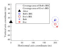
(a) Network topology and placement of elements.

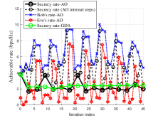
(b) Achievable rate vs. iteration index: The continuous domain for phase shifting elements.

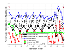
(c) Achievable rate vs. iteration index: The discrete domain for phase shifting elements.

Figure 2: The secrecy/receivers data rate over AO and GDA iterations.

We evaluate the convergence and performance of AO and GDA. We set $M=3$, $N_{\text{B}}=N_{\text{E}}=4$, $P=46$ dBm, $5$ MHz wireless band, and AWGN power density $-174$ dBm/Hz. The path loss exponents for the direct and reflected channels are set to $4$ and $2$, respectively. We apply the MIMO channel correlation model in [23] for the channels between Alice to each IRS. In the following, we consider the case that these MIMO channels are full-rank. For Gaussian randomization, we generate $10,000$ random vectors according to the optimized covariance matrix.

Fig. 2(b) shows the convergence behavior of AO and GDA for the continuous domain of phase shifting strategies. Within each AO iteration, we observe that after optimizing $\mathbf{w}$ and $\Theta_{\text{B}}$, the secrecy rate is non-decreasing. On the other hand, the secrecy rate is non-increasing after optimizing $\Theta_{\text{E}}$ at each AO iteration, verifying the feasibility of our adopted SDR techniques. Although AO may achieve better performance than GDA in some iterations, it does not guarantee convergence in general. This is due to the fact that for any given $\mathbf{w}$ and $\Theta_{\text{B}}$, optimizing $\Theta_{\text{E}}$ effectively changes the phase of Eve’s equivalent channel $\mathbf{h}_{\text{E}}\left(\mathbf{\Theta}_{\text{B}},\mathbf{\Theta}_{\text{E}}\right)$, specifically when the norm of Eve’s IRS channel dominates other channels, i.e., $\left\lVert\mathbf{h}_{\text{$\text{I}_{\text{E}}$,E}}\mathbf{\Theta}_{\text{E}}\mathbf{h}_{\text{A,$\text{I}_{\text{E}}$}}\right\rVert\gg\left\lVert\mathbf{h}_{\text{A,E}}\right\rVert$, and $\left\lVert\mathbf{h}_{\text{$\text{I}_{\text{E}}$,E}}\mathbf{\Theta}_{\text{E}}\mathbf{h}_{\text{A,$\text{I}_{\text{E}}$}}\right\rVert\gg\left\lVert\mathbf{h}_{\text{$\text{I}_{\text{B}}$,E}}\mathbf{\Theta}_{\text{B}}\mathbf{h}_{\text{A,$\text{I}_{\text{B}}$}}\right\rVert$. When Bob is close to Eve’s IRS, $\mathbf{\Theta}_{\text{E}}$ can effectively change the phase of Bob’s equivalent channel $\mathbf{h}_{\text{B}}\left(\mathbf{\Theta}_{\text{B}},\mathbf{\Theta}_{\text{E}}\right)$, such that it seriously degrades secrecy rate, due to the fixed $\mathbf{w}$. Hence, when $\left\lVert\mathbf{h}_{\text{$\text{I}_{\text{E}}$,B}}\mathbf{\Theta}_{\text{E}}\mathbf{h}_{\text{A,$\text{I}_{\text{E}}$}}\right\rVert\gg\left\lVert\mathbf{h}_{\text{A,B}}\right\rVert$, and $\left\lVert\mathbf{h}_{\text{$\text{I}_{\text{E}}$,B}}\mathbf{\Theta}_{\text{E}}\mathbf{h}_{\text{A,$\text{I}_{\text{E}}$}}\right\rVert\gg\left\lVert\mathbf{h}_{\text{$\text{I}_{\text{B}}$,B}}\mathbf{\Theta}_{\text{B}}\mathbf{h}_{\text{A,$\text{I}_{\text{B}}$}}\right\rVert$, we observe that Eve’s IRS may act as a jammer to Bob by changing the phase of $\mathbf{h}_{\text{B}}\left(\mathbf{\Theta}_{\text{B}},\mathbf{\Theta}_{\text{E}}\right)$ rather than enhancing $\mathbf{h}_{\text{E}}\left(\mathbf{\Theta}_{\text{B}},\mathbf{\Theta}_{\text{E}}\right)$. A similar effect can be observed at Bob’s IRS. The convergence behavior of GDA is smoother than AO such that after few iterations, it converges to a stationary point. Fig. 2(b) shows the convergence behavior of AO and GDA for $L_{\text{B}}=L_{\text{E}}=5$. Discrete domains for $\mathbf{\Theta}_{\text{B}}$ and $\mathbf{\Theta}_{\text{E}}$ usually improves the convergence of AO. This effect is because $\mathbf{\Theta}_{\text{E}}$ cannot be effectively chosen under a discrete domain. Although the same argument holds for $\mathbf{\Theta}_{\text{B}}$, the beamforming at Alice with a continuous domain can effectively compensate the inflexibility of choosing $\mathbf{\Theta}_{\text{B}}$. From numerical results, we observed that AO with discrete domains for $\mathbf{\Theta}_{\text{B}}$ and $\mathbf{\Theta}_{\text{E}}$ has smoother convergence than that of the continuous one, although it does not always hold. In the game-theoretic approach, the game has a single mixed NE. At that mixed NE, it is interesting to note that only five phase shift combinations share the whole probability mass of the optimal strategy for Bob and Eve. Following that strategy yields a mixed secrecy capacity of $6.436$ bps/Hz, which is higher than those of AO and GDA. In the game-theoretic approach, the priority of updating $\mathbf{\Theta}_{\text{E}}$ after optimizing $\mathbf{w}$ is not considered, so the optimal beamforming can effectively deteriorate Eve’s rate.

V Conclusion

We consider a wiretap channel where both the legitimate receiver and the eavesdropper use their own IRSs. We formulate a max-min secrecy rate problem, to design the transmit beamforming and phase shifting strategies of the IRSs by AO, GDA, and mixed NE. Simulation results show that AO does not guarantee convergence for continuous phase shifting, although it may achieve better performance than GDA in some iterations. GDA usually converges to a stationary point. Discrete phase shifting improves the convergence behavior of AO and GDA. The mixed NE strategy (with no priority among the players) achieves higher secrecy rate compared to AO and GDA.

Appendix A Derivation of $\nabla_{\mathbf{\Theta}_{\text{B}}}f$ in (III-B)

We first re-express $\mathbf{\bar{H}}_{\text{E2}}$ from (26) as follows:

$$\mathbf{\bar{H}}_{\text{E2}}\left(\mathbf{\Theta}_{\text{B}}\right):= \begin{bmatrix}\mathbf{c_{0}}&\mathbf{d}\\ \mathbf{d}^{H}&{0}\end{bmatrix},$$ (32)

where $\mathbf{d}=\mathbf{A}(\mathbf{a}+\mathbf{B}\mathbf{\Theta}_{\text{B}}\mathbf{c})\in\mathds{C}^{M\times 1}$, $\mathbf{A}=\text{diag}\left(\mathbf{h}^{*}_{\text{$\text{I}_{\text{E}}$,E}}\right)\mathbf{h}^{*}_{\text{A,$\text{I}_{\text{E}}$}}\mathbf{w}^{*}\mathbf{w}^{T}$ and $\mathbf{B}=\mathbf{h}^{T}_{\text{A,$\text{I}_{\text{B}}$}}$ are defined below (28), $\mathbf{a}=\mathbf{h}_{A,E}^{T}$ and $\mathbf{c}=\mathbf{h}_{I_{B},E}^{T}$ are both column vectors. Then, $\text{tr}\left(\mathbf{\bar{H}}_{\text{E2}}\left(\mathbf{\Theta}_{\text{B}}\right)\mathbf{\tilde{\Theta}}_{\text{E}}\right)$ can be rearranged as follows:

$$\text{tr}\left(\mathbf{\bar{H}}_{\text{E2}}\left(\mathbf{\Theta}_{\text{B}}\right)\mathbf{\tilde{\Theta}}_{\text{E}}\right)$$

$$=\lambda_{2}\text{tr}\left(\begin{bmatrix}\mathbf{c_{0}}&\mathbf{d}\\ \mathbf{d}^{H}&{0}\end{bmatrix}\begin{bmatrix}\mid&&\mid&\mid\\ \theta_{1}^{E*}\boldsymbol{\bar{\theta}_{\text{E}}}&\cdots&\theta_{N_{E}}^{E*}\boldsymbol{\bar{\theta}_{\text{E}}}&\boldsymbol{\bar{\theta}_{\text{E}}}\\ \mid&&\mid&\mid\end{bmatrix}\right)$$ (33)

$$=\lambda_{2}\text{tr}\left(\begin{bmatrix}\mathbf{c_{0}}&\mathbf{d}\\ \mathbf{d}^{H}&{0}\end{bmatrix}\begin{bmatrix}\theta_{1}^{E*}\boldsymbol{\theta_{\text{E}}}&\cdots&\theta_{N_{E}}^{E*}\boldsymbol{\theta_{\text{E}}}&\boldsymbol{\theta_{\text{E}}}\\ \theta_{1}^{E*}&&\theta_{N_{E}}^{E*}&1\end{bmatrix}\right)$$ (34)

$$=\lambda_{2}\left(\left(\sum_{k=1}^{N_{E}}\theta_{k}^{E*}\mathbf{c_{0,k}}\right)\boldsymbol{\theta_{\text{E}}}+\mathbf{d}^{T}\boldsymbol{\theta_{\text{E}}}^{*}+\mathbf{d}^{H}\boldsymbol{\theta_{\text{E}}}\right)$$ (35)

$$=\lambda_{2}\left(\tilde{{c}}_{0}+\boldsymbol{\theta_{\text{E}}}^{H}\mathbf{d}+\boldsymbol{\theta_{\text{E}}}^{T}\mathbf{d}^{*}\right),$$ (36)

where (33) and (34) are by definition of $\mathbf{\tilde{\Theta}}_{\text{E}}$ and $\boldsymbol{\bar{\theta}_{\text{E}}}$, respectively. In (35), we define $\mathbf{c_{0,k}}$ as the $k$-th row of $\mathbf{c_{0}}$. In (36), we define the first term inside the bracket in (35) as $\tilde{\mathbf{c}}_{0}$.

Then from (36) we have

$$\nabla_{\boldsymbol{\Theta_{\text{B}}}} \text{tr}\left(\mathbf{\bar{H}}_{\text{E2}}\left(\mathbf{\Theta}_{\text{B}}\right)\mathbf{\tilde{\Theta}}_{\text{E}}\right)=\lambda_{2}\frac{d}{d\boldsymbol{\Theta_{\text{B}}}^{*}}\left(\tilde{{c}}_{0}+\boldsymbol{\theta_{\text{E}}}^{H}\mathbf{d}+\boldsymbol{\theta_{\text{E}}}^{T}\mathbf{d}^{*}\right)$$ (37)

$$=\lambda_{2}\frac{d}{d\boldsymbol{\Theta_{\text{B}}}^{*}}\boldsymbol{\theta}_{\text{E}}^{H}\mathbf{d}^{*}$$ (38)

$$=\lambda_{2}\frac{d}{d\boldsymbol{\Theta_{\text{B}}}^{*}}\boldsymbol{\theta}_{\text{E}}^{H}\mathbf{A}^{*}(\mathbf{a}^{*}+\mathbf{B}^{*}\boldsymbol{\Theta_{\text{B}}}^{*}\mathbf{c}^{*})$$ (39)

$$=\lambda_{2}\frac{d}{d\boldsymbol{\Theta_{\text{B}}}^{*}}\mbox{tr}\left(\mathbf{A}^{*}(\mathbf{a}^{*}+\mathbf{B}^{*}\boldsymbol{\Theta_{\text{B}}}^{*}\mathbf{c}^{*})\boldsymbol{\theta}_{\text{E}}^{H}\right)$$ (40)

$$=\lambda_{2}\frac{d}{d\boldsymbol{\Theta_{\text{B}}}^{*}}\mbox{tr}\left(\mathbf{c}^{*}\boldsymbol{\theta}_{\text{E}}^{H}\mathbf{A}^{*}\mathbf{B}^{*}\boldsymbol{\Theta_{\text{B}}}^{*}\right)$$ (41)

$$={\lambda_{2}}\mathbf{B}^{H}\mathbf{A}^{H}\boldsymbol{\theta}_{\text{E}}^{*}\mathbf{c}^{H},$$ (42)

where (37) is from [21, (4.48)], (38) is due to the fact that $\tilde{\mathbf{c}}_{0}$, $\boldsymbol{\theta}_{\text{E}}$ and $\mathbf{d}$ do not contain $\boldsymbol{\Theta_{\text{B}}}^{*}$, (39) is due to the fact that $\mathbf{r}^{T}\cdot\mathbf{s}=\mbox{tr}(\mathbf{r}^{T}\cdot\mathbf{s})=\mbox{tr}(\mathbf{s}\cdot\mathbf{r}^{T}),$ where $\mathbf{r}$ and $\mathbf{s}$ are column vectors, (40) is due to the property $\mbox{tr}(\mathbf{P}\mathbf{Q})=\mbox{tr}(\mathbf{Q}\mathbf{P})$ and also $\mathbf{a}^{*}$ and $\mathbf{A}^{*}$ are not functions of $\boldsymbol{\Theta_{\text{B}}}^{*}$, (42) is due to the property $\frac{d}{d\mathbf{Z}^{*}}\mbox{tr}(\mathbf{P}\mathbf{Z}^{*})=\mathbf{P}^{T}$ [21, Table 4.3]. The gradient of the second term in $f$ is as follows:

$$\lambda_{2}\nabla_{\mathbf{\Theta}_{\text{B}}}\mathbf{\bar{h}}_{\text{E2}}\left(\mathbf{\Theta}_{\text{B}}\right)=\lambda_{2}\nabla_{\mathbf{\Theta}_{\text{B}}}\mbox{tr}\left[\mathbf{\bar{h}}_{\text{E2}}\left(\mathbf{\Theta}_{\text{B}}\right)\right]$$ (43)

$$=\frac{\lambda_{2}}{\sigma_{E}^{2}}\nabla_{\mathbf{\Theta}_{\text{B}}}\mbox{tr}\left[\left(\mathbf{h}_{\text{A,E}}+\mathbf{h}_{\text{$\text{I}_{\text{B}}$,E}}\mathbf{\Theta}_{\text{B}}\mathbf{h}_{\text{A,$\text{I}_{\text{B}}$}}\right)^{*}\mathbf{Q}\left(\mathbf{h}_{\text{A,E}}+\mathbf{h}_{\text{$\text{I}_{\text{B}}$,E}}\mathbf{\Theta}_{\text{B}}\mathbf{h}_{\text{A,$\text{I}_{\text{B}}$}}\right)^{T}\right]$$ (44)

$$=\frac{\lambda_{2}}{\sigma_{E}^{2}}\nabla_{\mathbf{\Theta}_{\text{B}}}\mbox{tr}\left[\left(\mathbf{h}_{\text{A,E}}+\mathbf{h}_{\text{$\text{I}_{\text{B}}$,E}}\mathbf{\Theta}_{\text{B}}\mathbf{h}_{\text{A,$\text{I}_{\text{B}}$}}\right)^{T}\left(\mathbf{h}_{\text{A,E}}+\mathbf{h}_{\text{$\text{I}_{\text{B}}$,E}}\mathbf{\Theta}_{\text{B}}\mathbf{h}_{\text{A,$\text{I}_{\text{B}}$}}\right)^{*}\mathbf{Q}\right]$$ (45)

$$=\frac{\lambda_{2}}{\sigma_{E}^{2}}\nabla_{\mathbf{\Theta}_{\text{B}}}\mbox{tr}\left[\mathbf{Q}\left(\mathbf{h}_{\text{A,E}}+\mathbf{h}_{\text{$\text{I}_{\text{B}}$,E}}\mathbf{\Theta}_{\text{B}}\mathbf{h}_{\text{A,$\text{I}_{\text{B}}$}}\right)^{T}\left(\mathbf{h}_{\text{A,E}}+\mathbf{h}_{\text{$\text{I}_{\text{B}}$,E}}\mathbf{\Theta}_{\text{B}}\mathbf{h}_{\text{A,$\text{I}_{\text{B}}$}}\right)^{*}\right]$$ (46)

$$= \frac{\lambda_{2}}{\sigma_{E}^{2}}\nabla_{\mathbf{\Theta}_{\text{B}}}\mbox{tr}\left[\mathbf{c}_{1}+\mathbf{c}_{2}\mathbf{\Theta}_{\text{B}}^{*}\right]$$ (47)

$$= \frac{\lambda_{2}}{\sigma_{E}^{2}}\mathbf{c}_{2}^{T},$$ (48)

where (43) is due to the fact that $\mathbf{\bar{h}}_{\text{E2}}\left(\mathbf{\Theta}_{\text{B}}\right)$ is a scalar, (44) is by definition (23), and (45) and (46) use tr$(\mathbf{A}\mathbf{B})$=tr$(\mathbf{B}\mathbf{A})$. In (47), $\mathbf{c}_{1}$ includes all term not relevant to $\boldsymbol{\Theta_{\text{B}}}^{*}$ and $\mathbf{c}_{2}:=\mathbf{h}_{\text{A,$\text{I}_{\text{B}}$}}^{*}\mathbf{Q}\left(\mathbf{h}_{\text{A,E}}+\mathbf{h}_{\text{$\text{I}_{\text{B}}$,E}}\mathbf{\Theta}_{\text{B}}\mathbf{h}_{\text{A,$\text{I}_{\text{B}}$}}\right)^{T}\mathbf{h}_{\text{$\text{I}_{\text{B}}$,E}}^{*}$. After combining (42) and (48), we have the gradient of $f$ with respect to $\mathbf{\Theta}_{\text{B}}$ as (28).

References

• [1] M. Di Renzo, M. Debbah, D.-T. Phan-Huy, A. Zappone, M.-S. Alouini, C. Yuen, V. Sciancalepore, G. C. Alexandropoulos, J. Hoydis, H. Gacanin, J. d. Rosny, A. Bounceur, G. Lerosey, and M. Fink, “Smart radio environments empowered by reconfigurable AI meta-surfaces: an idea whose time has come,” EURASIP Journal on Wireless Communications and Networking, May 2019.
• [2] M. Di Renzo, A. Zappone, M. Debbah, M.-S. Alouini, C. Yuen, J. de Rosny, and S. Tretyakov, “Smart radio environments empowered by reconfigurable intelligent surfaces: How it works, state of research, and the road ahead,” IEEE Journal on Selected Areas in Communications, vol. 38, no. 11, pp. 2450–2525, 2020.
• [3] N. S. Perović, L.-N. Tran, M. Di Renzo, and M. F. Flanagan, “Achievable rate optimization for MIMO systems with reconfigurable intelligent surfaces,” IEEE Transactions on Wireless Communications, vol. 20, no. 6, pp. 3865–3882, 2021.
• [4] H. Shen, W. Xu, S. Gong, Z. He, and C. Zhao, “Secrecy rate maximization for intelligent reflecting surface assisted multi-antenna communications,” IEEE Communications Letters, vol. 23, no. 9, pp. 1488–1492, 2019.
• [5] M. Cui, G. Zhang, and R. Zhang, “Secure wireless communication via intelligent reflecting surface,” IEEE Wireless Communications Letters, vol. 8, no. 5, pp. 1410–1414, 2019.
• [6] Z. Chu, W. Hao, P. Xiao, and J. Shi, “Intelligent reflecting surface aided multi-antenna secure transmission,” IEEE Wireless Communications Letters, vol. 9, no. 1, pp. 108–112, 2020.
• [7] H.-M. Wang, J. Bai, and L. Dong, “Intelligent reflecting surfaces assisted secure transmission without eavesdropper’s CSI,” IEEE Signal Processing Letters, vol. 27, pp. 1300–1304, 2020.
• [8] L. Dong and H.-M. Wang, “Secure MIMO transmission via intelligent reflecting surface,” IEEE Wireless Communications Letters, vol. 9, no. 6, pp. 787–790, 2020.
• [9] X. Yu, D. Xu, Y. Sun, D. W. K. Ng, and R. Schober, “Robust and secure wireless communications via intelligent reflecting surfaces,” IEEE Journal on Selected Areas in Communications, vol. 38, no. 11, pp. 2637–2652, 2020.
• [10] S. Hong, C. Pan, H. Ren, K. Wang, and A. Nallanathan, “Artificial-noise-aided secure MIMO wireless communications via intelligent reflecting surface,” IEEE Transactions on Communications, vol. 68, no. 12, pp. 7851–7866, 2020.
• [11] H. Niu, Z. Chu, F. Zhou, Z. Zhu, M. Zhang, and K.-K. Wong, “Weighted sum secrecy rate maximization using intelligent reflecting surface,” IEEE Transactions on Communications, vol. 69, no. 9, pp. 6170–6184, 2021.
• [12] B. Feng, Y. Wu, M. Zheng, X.-G. Xia, Y. Wang, and C. Xiao, “Large intelligent surface aided physical layer security transmission,” IEEE Transactions on Signal Processing, vol. 68, pp. 5276–5291, 2020.
• [13] Z. Chu, W. Hao, P. Xiao, D. Mi, Z. Liu, M. Khalily, J. R. Kelly, and A. P. Feresidis, “Secrecy rate optimization for intelligent reflecting surface assisted MIMO system,” IEEE Transactions on Information Forensics and Security, vol. 16, pp. 1655–1669, 2021.
• [14] P. Staat, H. Elders-Boll, M. Heinrichs, C. Zenger, and C. Paar, “Mirror mirror on the wall: Wireless environment reconfiguration attacks based on fast software-controlled surfaces,” https://arxiv.org/abs/2107.01709.
• [15] B. Lyu, D. T. Hoang, S. Gong, D. Niyato, and D. I. Kim, “IRS-based wireless jamming attacks: When jammers can attack without power,” IEEE Wireless Communications Letters, vol. 9, no. 10, pp. 1663–1667, 2020.
• [16] S. Zhang and R. Zhang, “Capacity characterization for intelligent reflecting surface aided MIMO communication,” IEEE Journal on Selected Areas in Communications, vol. 38, no. 8, pp. 1823–1838, 2020.
• [17] Q. Wu and R. Zhang, “Beamforming optimization for wireless network aided by intelligent reflecting surface with discrete phase shifts,” IEEE Transactions on Communications, vol. 68, no. 3, pp. 1838–1851, 2020.
• [18] L. Liu, R. Zhang, and K.-C. Chua, “Secrecy wireless information and power transfer with MISO beamforming,” IEEE Transactions on Signal Processing, vol. 62, no. 7, pp. 1850–1863, 2014.
• [19] A. Khisti and G. W. Wornell, “Secure transmission with multiple antennas I: The MISOME wiretap channel,” IEEE Transactions on Information Theory, vol. 56, no. 7, pp. 3088–3104, 2010.
• [20] Q. Wu and R. Zhang, “Intelligent reflecting surface enhanced wireless network via joint active and passive beamforming,” IEEE Transactions on Wireless Communications, vol. 18, no. 11, pp. 5394–5409, 2019.
• [21] A. Hjorungnes, Complex-Valued Matrix Derivatives: With Applications in Signal Processing and Communications.   Cambridge University Press, 2011.
• [22] C. E. Lemke and J. T. Howson, Jr., “Equilibrium points of bimatrix games,” Journal of the Society for Industrial and Applied Mathematics, vol. 12, no. 2, pp. 413–423, 1964. [Online]. Available: https://doi.org/10.1137/0112033
• [23] A. Sayeed, “Deconstructing multiantenna fading channels,” IEEE Transactions on Signal Processing, vol. 50, no. 10, pp. 2563–2579, 2002.