Sensitivity of the MnTe valence band to orientation of magnetic moments

Abstract

An effective model of the hexagonal (NiAs-structure) manganese telluride valence band in the vicinity of the A-point of the Brillouin zone is derived. It is shown that while for the usual antiferromagnetic order (magnetic moments in the basal plane) band splitting at A is small, their out-of-plane rotation enhances the splitting dramatically (to about 0.5 eV). We propose extensions of recent experiments (Moseley et al., Phys. Rev. Materials 6, 014404) where such inversion of magnetocrystalline anisotropy has been observed in Li-doped MnTe, to confirm this unusual sensitivity of a semiconductor band structure to magnetic order.

I Introduction

The electronic structure of crystalline semiconductors can be treated by various methods which differ greatly in their computational cost.someBook Among ab initio methods, GW is one of the most advanced approaches yet a numerically rather expensive one.Grumet:2018_a A widely-used alternative is density functional theory (DFT) where the speed comes at the cost of worse performance (even if there are various approaches to mitigate deficiencies such as too small gaps) and yet faster options are available, of which tight-binding approachesAndersen:1984_a and $k\cdot p\$modelsWinkler2003 will be of interest here. Such effective models need material parameters (such as on-site energies or hopping amplitudes) as an input which can sometimes be of advantage because they can be adjusted to fit experiments. Also, they may offer insight into mechanisms governing the band structure.

An archetypal example of an effective model is the Kohn-Luttinger HamiltonianLuttinger:1956_a which has a wide range of applications to non-magnetic materials, including silicon and III-V semiconductors with $\Gamma_{8}$ manifold at the top of the valence band (VB). Magnetism adds a new twist: for Mn-doped GaAs, the host is described by this Hamiltonian and the effect of ferromagnetic ordering is captured by a kinetic $pd$ exchange term $\propto\hat{\vec{s}}\cdot\vec{S}$ where $\hat{\vec{s}}$ is the spin operator (of the VB holes) and $\vec{S}$ is the classical spin representing the Mn magnetic moments (usually treated on the mean-field level). Such description of ferromagnetic semiconductorsTanaka:2021_a ; Jungwirth:2014_a has been employed extensively in the context of spintronicsMarrows:2011_a and now that antiferromagnetic spintronicsBaltz:2018_a has become an active field, we hereby wish to contribute to its progress by presenting an effective model of hexagonal (NiAs-structure) MnTe which is a well-established antiferromagnetic semiconductor, as exemplified by its $T=0$ band structure in Fig. 1, with a relatively high ($\approx 310$ K) Néel temperature. Typical samples, both bulk and layers exhibit p-type conductivity and we will therefore focus on its VB.

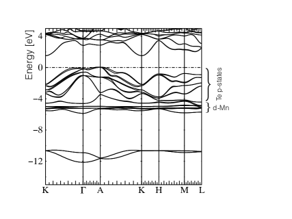
Figure 1: Band structure of MnTe calculated by QSGW for $\vec{L}\perp z$ (in-plane orientation). Note the competing maxima of the valence band at $\Gamma$ and $A$ points.

The magnetic structure of MnTe was establishedKomatsubara:1963_a long ago (see Fig. 3) with a strong anisotropy favouring in-plane orientation of the magnetic moments and a weak residual anisotropy within the plane.Kriegner:2017_a Recently, Moseley et al. Moseley:2022_a have found by neutron diffraction that, upon doping by lithium, the magnetic moments rotate out of plane. They also noticed that in the density of states (DOS), significant changes occur and we use the effective model to explain how the VB responds to this change of magnetic order (once spin-orbit interaction is taken into account). Even if the Mn $d$-states lieSato:1994_a deep below the Fermi level $E_{F}$ and seem too remote from the VB topBossini:2020_a which is built dominantly from $p$-Te orbitals, we demonstrate that the combination of MnTe layered structure and relativistic spin-orbit interaction (SOI) lead to an unusual sensitivity of the electronic structure to the orientation of magnetic moments. In the next Section we discuss the competing VB maxima and we focus on the one near A-point of the Brillouin zone (BZ) in Sec. III. We conclude in Sec. IV.

II Competing VB maxima

Once the SOI is taken into account, there arises a tight competition between valence band maxima close to A and $\Gamma$ points of the BZ, see Fig. 2b. A long-standing consensusPodgorny:1983_a ; note3 that the former prevails has recently been challenged by Yin et al. [Yin:2019_a, ] who claim that the VB top occurs in the vicinity of $\Gamma$ point. To improve on the potentially less accurate DFT approach,Yin:2019_a we employ the Quasiparticle Self-Consistent GW approximationKotani:2007_a (QSGW). The GW approximation, which is an explicit theory of excited states is widely used to predict quasiparticle levels with better reliability than density functionals. QSGW is an optimized form of the GW approximation, where the starting Hamiltonian is generated within the GW approximation itself, constructed so that it minimizes the difference between the one-body and many-body Hamiltonians. As a by-product the poles of the one-body Green’s function coincide with the poles of the interacting one: thus energy band structures have physical interpretation as quasiparticle levels, in marked contrast to DFT approaches (some examples are given in Sec. 5.1 of the Supplementary Information) where the auxillary Hamiltonian has no formal physical meaning (in practice Lagrange multipliers of this Hamiltonian are interpreted as quasiparticle levels). In practice QSGW yields high fidelity quasiparticle levels in most materials where dynamical spin fluctuations are not strong.Schilfgaarde:2006_a

Bulk lattice constants of MnTe at room temperature are $a=0.414$ nm and $c=0.671$ nm;Moseley:2022_a we show in Fig. 2d that for such $c/a=1.621$, the VB maximum close to the A point safely prevails ($\Delta E$ is the difference between energy of local VB maxima close to $\Gamma$ and that close to $A$). Most experiments nowadays are performed with thin films of MnTe, however, and then lattice constants depend on the choice of substrate. Temperature-dependent data in Fig. 3 of Ref. Kriegner:2017_a, suggest that while samples grown on SrF₂ surface still fall into the same class, low temperatures may effectively push the VB maxima close to the $\Gamma$ point up and in particular, samples grown on the InP substrate may exhibit the inverted alignment of the VB maxima.

Comparing the present QSGW results to DFT calculations of Ref. Yin:2019_a, , several remarks are in order. Lattice constants used in that reference (which correspond to $c/a=1.57$) have been obtained by structure optimisation in DFT rather than from experimental data. Next, the hybrid functional HSE06 may avoid the known problem of underestimated gaps in DFT but this in itself does not guarantee a reliable description of finer details of the band structure (such as VB maxima alignment). Predicted valence and conduction bands are more uniformly reliable in GW than in density-functional methods. Moreover QSGW surmounts the problematic starting-point dependence that plagues the usual implementations of the GW approximation and therefore QSGW is a better choice for our study than DFT. Regarding the subsequent derivation of an effective model for the VB around $\Gamma$ point,Yin:2019_a we note as follows. The $k_{z}=0$ approximation is used; while this would be appropriate for very thin layers (say 5 nm), present experiments Kriegner:2017_a are more likely behaving like 3D bulk. Also, the effective model (1) in Ref. Yin:2019_a, assumes a fixed direction of the magnetic moments; to plot the experimentally relevant ’angular sweeps’, the current direction rather than Néel vector is rotated which is, however, not the actual experimental protocol. For systems where only the non-crystalline anisotropic magnetoresistance (AMR) occurs,Rushforth:2007_a the two protocols are equivalent but measurements in the Corbino geometryKriegner:2017_a prove this assumption false. Being aware of these issues, we strive to derive an effective model in the following which is free of these shortcomings captures the dependence on magnetic moments direction.

(a)	(b)
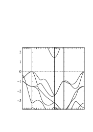
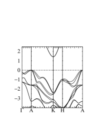
(c)	(d)

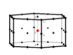
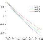
Figure 2: Detailed view of the VB maximum and (c) the Brillouin zone of $\alpha$-MnTe corresponding to lattice constants: 0.414 nm and $c/a=1.6208$. Panels (a,b) show the difference between SOI ignored and included and (d) gives for the latter case the energy difference between VB maximum in $\Gamma$ and A depending on the $c/a$ ratio (for several values of $a$ given in a.u.); origin of this dependence is discussed in Sec. 5.2 of the Supplementary Material. Negative $\Delta E$ means that the VB maxima around A prevail and all energies are given in eV.

A proper symmetry analysis of the crystal structure of MnTe provides the non-symmorphic space group D${}_{\text{6h}}^{\text{4}}$. Once AF ordering is included the Mn atoms must be treated as inequivalent since each Mn layer would have spins pointing in the opposite direction as shown in Fig. 3 for in-plane spins. Hence, the symmetry group is reduced from D${}_{\text{6h}}$ to D${}_{\text{3d}}$ without SOI (see for instance Sandratskii et al.Sandratskii:1981_a ). Furthermore, the symmetry group would also depend on the interplay of SOI and choice of the AF direction since spins pointing in different directions behave differently under symmetry operations. For example, in the out-of-plane AF configuration, the symmetry remains D${}_{\text{3d}}$ while for in-plane AF, either along $\left[10\bar{1}0\right]$ or $\left[11\bar{2}0\right]$ directions, the symmetry group is reduced C${}_{\text{2h}}$. Besides the conceptual analysis of the symmetries, independent calculations using the WIEN2k and Quantum Espresso ab initio packages also provide the same symmetry groups discussed above. Thus, for the particular choice of in-plane AF the D${}_{\text{2h}}$ point group discussed by Yin et al. should be replaced by C${}_{\text{2h}}$.

III Effective models

Several attempts to describe the electronic structure of $\alpha$-MnTe in a simplified way have been made so far. Here, the $k\cdot p$ approachWinkler2003 ; LewYanVoon2009 is a common choice for semiconductorsFariaJunior2016PRB especially if only high-symmetry points in the BZ are of interest. Such a model for the VB top in A point was derived more than 40 years agoSandratskii:1981_a and later extended to a tight-binding scheme.Masek:1987_a The latter allows for the description of the energy bands over the whole BZ but neither of these models allows to analyse the dependence of electronic structure on the directions on Mn magnetic moments. In the perfectly ordered AFM phase (as in Fig. 2d) and without SOI, the Bloch functions at the top of the valence band in the A point transform as the two-dimensional irreducible representation E${}_{\text{g}}$ or ($\Gamma_{3}^{+}$) of the the D_3d. Including corrections up $k^{2}$ and no SOI (essentially given by Eq. 2 in Sandratskii et al.Sandratskii:1981_a ) one would obtain the following Hamiltonian:

$$H_{kp,2\times 2}=\left(\begin{array}[]{cc}ak_{x}^{2}+bk_{y}^{2}+ck_{z}^{2}&(a-b)k_{x}k_{y}\\ (a-b)k_{x}k_{y}&bk_{x}^{2}+ak_{y}^{2}+ck_{z}^{2}\end{array}\right)\,.$$ (1)

The inverse effective masses (proportional to $a,b,c$) imply that Fermi surfaces (FSs) are, at this level of approximation, two prolate ellipsoids (both doubly degenerate) touching at the point where they are pierced by the A$\Gamma$ line; other properties of this model and its parameters, effective masses, extracted from fits to QSGW are given in Sec. 2 of the Supplementary Material. From the point of view of magnetism, this is a consequence of neglecting the spin-orbit interaction. Once SOI is included, the band dispersion will depend on the direction of magnetic moments. On the other hand, if higher order terms in $\vec{k}$ were included, the symmetry would be lowered and FSs would become warped and spin-split.Smejkal:2021_a Consequent spin order in reciprocal space, being a hallmarkMazin:2021_a of so called altermagnetism, can lead to phenomena normally unexpected in collinear compensated magnets such as the anomalous Hall effect.

The derivation of Eq. (1) is based solely on symmetry arguments and entails neither any explicit information about orbital composition of the corresponding Bloch states nor any parametric dependence on magnetic order. In the following, we therefore first describe a toy model capturing the essence of interplay between magnetism and orbital degrees of freedom and next, we make use of these insights to derive a realistic model of MnTe.

III.1 Toy model

Consider a 1D chain of alternating nonmagnetic (A) and magnetic (B) atoms depicted in Fig. 3 where only the nearest neighbours couple (the amplitude being $t$). The single-orbital-per-site tight-binding Hamiltonian assuming that the B-atom orbitals have on-site energies $\epsilon_{d}\pm\Delta$ (where $2\Delta$ is the exchange splitting) reads

$$H_{1}(\Delta)=\left(\begin{array}[]{cccc}0&t&0&te^{-ika}\\ t&\epsilon_{d}+\Delta&t&0\\ 0&t&0&t\\ te^{ika}&0&t&\epsilon_{d}-\Delta\end{array}\right)$$ (2)

in the basis of Bloch states with momentum $k$ so that $ka$ ranging from $-\pi$ to $\pi$ parametrises the BZ.

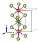
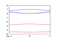
Figure 3: NiAs structure (left) reduced to a toy model comprising a one-dimensional chain of magnetic (B) and non-magnetic (A) atoms; there are two of the latter, A_a and A_b per unit cell. Energies are shown in the units of $t$ and $\Delta/t=1$, $-\epsilon_{d}/t=3$ was chosen.

The toy model described by $H_{1}$ can be treated analytically (see Ref. [SI, ], Sec. 1) and focusing on the bands of dominantly A-atom orbital composition, we observe a downfolded cosine band of width downscaled by factor $\approx t/\epsilon_{d}$ in the large $|\epsilon_{d}|$ limit, i.e. remote B-atom dominated bands, as the dashed black dispersion in Fig. 3 confirms. Atoms A_a and A_b interact only through the intermediate (magnetic) atoms $B$ which suppresses their effective coupling. There are two main observations to make at this point. First, even if $\Delta\ll\epsilon_{d}$ there opens a gap in the ’VB states’ at the BZ edge (to make the gap better visible, we chose a larger value of $\Delta/\epsilon_{d}$ for the blue and red bands in Fig. 3). This allows for the insight that, inasmuch the atom A_b is sandwiched between spin-up (left) and spin-down neighbours (right), where the exchange coupling is $\Delta$ and $-\Delta$, their effect on the A-band (blue in Fig. 3 at the bottom right panel) does not average out to zero. Next, an even more important insight concerns the eigenstates of $H_{1}$ at $ka=\pm\pi$.

At this point, we should point out that $H_{1}$ of (2) in fact only describes one of the two spin species; let us denote it as up-spin and correspondingly, $H_{1,\uparrow}=H_{1}(\Delta)$. The two states at $ka=\pm\pi$ split by nonzero $\Delta$ turn out to be $(|a\rangle\pm|b\rangle)\otimes|\uparrow\rangle$ where $|a\rangle$ and $|b\rangle$ refer to orbitals of A_a and A_b atoms, respectively. For the spin-down sector, $H_{1,\downarrow}=H_{1}(-\Delta)$ which leads to identical band structure as in Fig. 3 whose eigenstates are nevertheless not the same as for $H_{1,\uparrow}$. The state degenerate with $(|a\rangle\pm|b\rangle)\otimes|\uparrow\rangle$ is $(|a\rangle\mp|b\rangle)\otimes|\downarrow\rangle$ and thus, we arrive at the conclusion that, at the BZ edge, the VB states in our toy model come in two pairs (split by the gap) and without loss of generality, we now focus on the subspace spanned by the pair

$$(|a\rangle+|b\rangle)\otimes|\!\!\uparrow\rangle,(|a\rangle-|b\rangle)\otimes|\!\!\downarrow\rangle.$$ (3)

Unlike the pair $|\!\!\uparrow\rangle,|\!\!\downarrow\rangle$ (without any orbital part), any linear combination of the two states in (3) has a zero expectation value of transversal spin operators $\hat{\sigma}_{x}$, $\hat{\sigma}_{y}$. This can also be restated as $\langle\hat{\vec{\sigma}}\rangle||z$, or, easily generalised to the statement that the states (3) have the (expectation value of) spin parallel to the magnetic moments of atoms B. In this way, the direction of magnetic moments of the atoms remote in energy from the VB top influences the current-carrying states close to the Fermi energy. In the following, we denote the direction of spin in the basis state $(|a\rangle+|b\rangle)\otimes|\!\!\uparrow\rangle$ by $\vec{L}$ and it can be understood as the Néel vector. In the following, we explore this influence in the context of spin-orbit interaction; an alternative pathway relies on spin disorderBaral:2022_a (as it occurs for example at finite temperatures) and we outline an approach to it based on the coherent potential approximation (CPA) in the Supplementary material. It provides an alternative interpretation of ’magnetic blue shift’ Bossini:2020_a of the gap which does not rely on many-body effects.

III.2 Extension to MnTe crystal

The previous argument can be extended to Te $p_{x}$, $p_{y}$ states which form the VB top near A. To account for fine details of the band structure (as explained in Ref. SI, , Sec. 2), we also include the remote $p_{z}$ levels (in A, they are $\approx 3$ eV below the VB top, see Fig. 2a) whose dispersion is dropped at this level of approximation. Also note that the group of VB maxima close to $\Gamma$ relies on Te $p_{z}$ orbitals as explained in the Supplementary material. We will measure energy from the VB top (as it appears in the case of absent SOI) with $E_{F}$ denoting the Fermi energy and use two copies of Eq. (1) to describe the $k_{x,y}$-dependent mixing of $p_{x}$, $p_{y}$ orbitals.

Denoting the position of $p_{z}$ orbitals of tellurium by $e_{z}$ ($e_{z}<0$, $|e_{z}/E_{F}|\gg 1$), the full description of the VB close to A is provided by a block-diagonal $6\times 6$ matrix

$$H_{kp}=\left(\begin{array}[]{cccccc}ak_{x}^{2}+bk_{y}^{2}+ck_{z}^{2}&(a-b)k_{x}k_{y}&0\\ (a-b)k_{x}k_{y}&bk_{x}^{2}+ak_{y}^{2}+ck_{z}^{2}&0\\ 0&0&e_{z}\\ &&&ak_{x}^{2}+bk_{y}^{2}+ck_{z}^{2}&(a-b)k_{x}k_{y}&0\\ &&&(a-b)k_{x}k_{y}&bk_{x}^{2}+ak_{y}^{2}+ck_{z}^{2}&0\\ &&&0&0&e_{z}\end{array}\right)$$ (4)

and the first and second $3\times 3$ block is written in the basis (3) whereas inside the blocks, the basis vectors are simply $|p_{x}\rangle,|p_{y}\rangle,|p_{z}\rangle$. Since the matrix (4) does not explicitly depend on $\vec{L}$ (only its basis vectors are), we arrive at the conclusion that (when SOI is ignored) the band structure does not depend on the direction of Mn magnetic moments.

In the limit $|e_{z}|\to\infty$, the full model (4) combined with SOI breaks down into two decoupled $2\times 2$ blocks and since we now have a microscopic understanding of the basis, one which contains the information about direction of Mn magnetic moments, the SOI can now be evaluated. With finite $e_{z}$, the dependence of band splitting in A can be better described as we explain in the following.

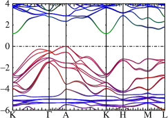
Figure 4: MnTe band structure for $\vec{L}||z$ (energies in eV). Colour coding: red Te, blue/green Mn.

III.3 Spin-orbit interaction

We are now in a position to explain the following behaviour of band structure calculated by relativistic ab initio methods. In panel (b) of Fig. 2, we could have already observed the bands split by SOI and, compared to band widths, such splittings were small (note that these splittings cause the shift of the VB top away from A, the point of high symmetry). Those calculations were done assuming $\vec{L}\parallel x$ and, at this level of detail, depend only little on the direction of $\vec{L}$ as long as $\vec{L}\perp z$ which is compatible with MnTe being an easy-plane material.Kriegner:2017_a However, when $\vec{L}\parallel z$ is assumed in calculations, see Fig. 4, band splittings become sizable. Restricting our discussion to Te $p_{x}$, $p_{y}$ orbitals combined into the states (3), this behaviour is linked to the directionality of $H_{so}=\lambda\vec{l}\cdot\vec{\sigma}$ evaluated in the corresponding basis:

$$H_{so,2\times 2}=\left(\begin{array}[]{cc}0&i\lambda\cos\theta\\ -i\lambda\cos\theta&0\end{array}\right)$$ (5)

where $\vec{L}\cdot\hat{z}=\cos\theta$ and $\vec{l}$ is the orbital angular momentum operator. Clearly, SOI projected to such a restricted space becomes ultimately ineffective for the in-plane orientation of magnetic moments where $\theta=\pi/2$ (taking into account also the $|p_{z}\rangle$ orbital,SI small splittings at Ain the in-plane configuration can nevertheless be also accounted for) whereas for finite $e_{z}$, the full $6\times 6$ matrix of $H_{so}$ must be considered instead of (5). On the other hand, for out-of-plane magnetic moments, the splitting at A seen in Fig. 4 can be directly compared to eigenvalues $\pm\lambda$ of $H_{so,2\times 2}$.

IV Discussion and conclusions

An effective model of the MnTe valence band around A point of the BZ depends on the level of detail needed: Eq. (1) is a meaningful approximation to begin with but it cannot describe the band-dispersion dependence on the direction of Mn magnetic moments; the six-band (or four-band, corresponding to $|e_{z}|\to\infty$ limit) description using Eq. (4) combined with $H_{so}$ evaluated with respect to basis (3) times $|p_{x}\rangle,|p_{y}\rangle,|p_{z}\rangle$ is the reasonable next step. On this level, the large sensitivity of the valence band at A to magnetic moment orientation can be explained in terms of zero matrix elements of $H_{so}$ between $(|a\rangle+|b\rangle)\otimes|\!\!\rightarrow\rangle$ and $(|a\rangle-|b\rangle)\otimes|\!\!\leftarrow\rangle$ where $a,b$ refer to the two Te atoms within unit cell of MnTe. Zooming into the details of the valence band smaller than $\sim 100$ meV would require adding further terms such as those discussed on p. 8 of the supplementary information to Ref. [Smejkal:2021_a, ]; on this level of approximation, phenomena such as the anomalous Hall effect or AMR can then likely be successfully modelled.

Calculations in Fig. 4 show that the splitting at A is associated with reduction of band gap in agreement with DFT calculations.Moseley:2022_a This implies that not only angular-resolved photoemission (ARPES) could be used to confirm the sensitivity of MnTe band structure to the orientation of Mn magnetic moments but also optical absorption measurements should reveal signatures of this effect. Such experiments could also confirm our results concerning the competition of valence band maxima close to the A and $\Gamma$ points of the Brillouin zone.

V Acknowledgements

We acknowledge assistance of Swagata Acharya with QSGW calculations and a preliminary KKR survey by Alberto Marmodoro; funding was provided by grants 22-21974S and EU FET Open RIA No. 766566, M.v.S. was supported by the DOE-BES Division of Chemical Sciences under Contract No. DE- AC36-08GO28308 and P.E.F.Jr. acknowledges financial support from the Alexander von Humboldt Foundation, Capes (Grant No. 99999.000420/2016-06) and Deutsche Forschungsgemeinschaft SFB 1277 (Project No. ID314695032, subprojects B05, B07 and B11).

References

- (1) Fabien Tran et al., J. Appl. Phys. 126, 110902 (2019)
- (2) M. Grumet et al., Phys. Rev. B 98, 155143 (2018).
- (3) O.K. Andersen and O. Jepsen, Phys. Rev. Lett. 53, 2571 (1984).
- (4) R. Winkler, Spin-orbit Coupling Effects in Two-Dimensional Electron and Hole Systems, (Springer, New York, 2003).
- (5) J. M. Luttinger, Phys. Rev. 102, 1030 (1956).
- (6) M. Tanaka, Jpn. J. Appl. Phys. 60, 010101 (2021).
- (7) T. Jungwirth et al., Rev. Mod. Phys. 86, 855 (2014).
- (8) C.H. Marrows and B.J. Hickey, Phil. Trans. R. Soc. A 369, 3027 (2011).
- (9) V. Baltz et al., Rev. Mod. Phys. 90, 015005 (2018).
- (10) Apart from the NiAs-type structure of MnTe, zinc-blende phase also exists which is AFM at low temperatures.
- (11) T. Komatsubara et al. ’63, doi: 10.1143/JPSJ.18.356
- (12) D. Kriegner et al., Phys. Rev. B 96, 214418 (2017).
- (13) D.H. Moseley et al., Phys. Rev. Mat. 6, 014404 (2022).
- (14) H. Sato et al., Sol. St. Comm. 92, 921 (1994).
- (15) R. Baral et al., Matter, 5, pp. 1853-1864 (2022).
- (16) D. Bossini et al., New J. Phys. 22, 083029 (2020).
- (17) M. Podgorny and J. Oleszkiewicz, J. Phys. C: Sol. St. Phys. 16, 2547 (1983).
- (18) More recent studies range from S. J. Youn et al., phys. stat. sol. (b) 241, 1411 (2004) to Mu et al., Phys. Rev. Mat. 3, 025403 (2019) and this VB maxima alignment is also consistent with our previous DFT+U calculations.Kriegner:2017_a
- (19) T. Kotani et al., Phys. Rev. B 76, 165106 (2007).
- (20) M. van Schilfgaarde and Takao Kotani and S. Faleev, Phys. Rev. Lett. 96, 226402 (2006).
- (21) G. Yin et al., Phys. Rev. Lett. 122, 106602 (2019).
- (22) A.W. Rushforth et al., Phys. Rev. Lett. 99, 147207 (2007).
- (23) L.M. Sandratskii et al., phys. stat. sol. (b) 104, 103 (1981).
- (24) L. C. Lew Yan Voon, M. Willatzen, The method: electronic properties of semiconductors, (Springer, Berlin, 2009).
- (25) P. E. Faria Junior et al., Phys. Rev. B 93, 235204 (2016).
- (26) J. Mašek, B. Velický and V. Janiš, J. Phys. C: Solid State Phys. 20, 59 (1987).
- (27) Libor Šmejkal, Jairo Sinova, and T. Jungwirth, Phys. Rev. X 12, 031042 (2022).
- (28) I. Mazin et al., Proceedings of Nat. Acad. Sci. USA 118 (42) e2108924118.
- (29) Supplementary information.