A new endstation for extreme-ultraviolet spectroscopy of free clusters and nanodroplets

Abstract

We present a new endstation for the AMOLine of the ASTRID2 synchrotron at Aarhus University, which combines a cluster and nanodroplet beam source with a velocity map imaging and time-of-flight spectrometer for coincidence imaging spectroscopy. Extreme-ultraviolet spectroscopy of free nanoparticles is a powerful tool for studying the photophysics and photochemistry of resonantly excited or ionized nanometer-sized condensed-phase systems. Here we demonstrate this capability by performing photoelectron-photoion coincidence (PEPICO) experiments with pure and doped superfluid helium nanodroplets. Different doping options and beam sources provide a versatile platform to generate various van der Waals clusters as well as He nanodroplets. We present a detailed characterization of the new setup and present examples of its use for measuring high-resolution yield spectra of charged particles, time-of-flight ion mass spectra, anion–cation coincidence spectra, multi-coincidence electron spectra and angular distributions. A particular focus of the research with this new endstation is on intermolecular charge and energy-transfer processes in heterogeneous nanosystems induced by valence-shell excitation and ionization.

I Introduction

Synchrotron radiation has been used to study the structure and dynamics of atoms, molecules and clusters since the 1980s. Nevertheless, synchrotron spectroscopy of gas-phase targets still is an active research field today, due to the advantages of synchrotrons over lasers and other light sources: The enormous range of photon energies covered by synchrotrons, spanning from the infrared up to hard X-rays, is unchallenged by any other radiation source. State-of-the-art monochromator beamlines typically provide extremely narrow-band radiation ($E/\Delta E>10^{4}$) continuously tunable across wide spectral ranges. This allows us to perform high-resolution spectroscopy in the extreme-ultraviolet (EUV) or X-ray ranges, not accessible by other means.

Over the past decades, the focus of gas-phase synchrotron science has been shifting from mere atomic and molecular structure determination to unraveling the complex photophysics and photochemistry of free biomolecules and nanoparticles. Atomic and molecular clusters are ideal model systems with reduced complexity that enable detailed studies of relaxation dynamics in condensed phase systems initiated by valence-shell or inner-shell excitation or ionization. In particular, interatomic or intermolecular charge and energy transfer are fundamentally important relaxation processes of weakly bound molecules and nanosystems exposed to ultraviolet up to X-ray radiation. Nanoparticles are of great interest for modern applications due to their peculiar properties determined by finite-size effects; applications range from heterogeneous photocatalysis Han et al. (2018), nanoplasmonics Liz-Marzán, Murphy, and Wang (2014), aerosol science Wang, Friedlander, and Mädler (2005), to radiation biology Butterworth et al. (2012).

Recent technical developments in synchrotron technology have mostly aimed to increase the achievable photon energy, brilliance and coherence of X-ray beams. In the particular field of gas-phase studies at synchrotrons, major progress has been made by devising more and more sophisticated diagnostic methods. Imaging detection of ions and electrons emitted by the irradiated molecules and nanoparticles provides both information about magnitudes and angles of electron and ion momenta. In particular, the velocity map imaging (VMI) technique Eppink and Parker (1997) is now widely used at EUV gas-phase beamlines because of its high particle momentum resolution and its $4\pi$-collection efficiency. Additionally, the combination of VMI of electrons with time-of-flight (TOF) detection of ions, or vice versa, or even double-sided VMI detection, where the electrons and ions are detected in coincidence (photoelectron-photoion coincidence, PEPICO), are established techniques at many facilities nowadays Garcia et al. (2005); Hosaka et al. (2006); Rolles et al. (2007); Tang et al. (2009); O’Keeffe et al. (2011); Garcia et al. (2013); Bodi et al. (2012); Tang et al. (2015); Kostko et al. (2017).

Gas-phase synchrotron science is also being moved forward by devising and implementing more diverse sources of free molecular complexes, clusters and nanoparticles into EUV and X-ray beamlines. While biologically relevant molecules are mostly thermally evaporated Prince et al. (2015), supersonic jet expansions are also used, where the carrier gas is bubbled through water and passed over the sample vapor to form microhydrated clusters Khistyaev et al. (2013). A slow-flow laser photolysis reactor in the vicinity of the ionization region is used to measure unimolecular and bimolecular reactions of free radicals Sztáray et al. (2017). Using the photon-ion merged-beams technique Schippers et al. (2016), highly charged ions Simon et al. (2010), size-selected metal clusters Niemeyer et al. (2012), and endohedral fullerenes have been investigated Kilcoyne et al. (2010). By coupling an aerosol source to a synchrotron beamline, particles up to a size of $\sim$1\text{\,}\mathrm{\SIUnitSymbolMicro m}$$ can be studied by EUV radiation Shu et al. (2006); Gaie-Levrel et al. (2011); Goldmann et al. (2015).

Another attractive target system for EUV synchrotron studies is pure and doped superfluid helium (He) nanodroplets (HNDs) Toennies and Vilesov (2004); Mudrich and Stienkemeier (2014). Pioneering work by the groups of Toennies Fröchtenicht et al. (1996), Möller von Haeften et al. (1997), and Neumark Ziemkiewicz, Neumark, and Gessner (2015), have revealed complex relaxation dynamics of resonantly excited He nanodroplets, including visible and EUV fluorescence emission von Haeften et al. (1997), autoionization causing the emission of ultraslow electrons Peterka et al. (2003), the ejection of mostly He2+ ions, and, to a lesser extent, larger fragment ions. Dopant molecules embedded inside the He droplets were found to be efficiently ionized indirectly by Penning-like excitation-transfer ionization via He^* ‘excitons’.Fröchtenicht et al. (1996); Wang et al. (2008); Peterka et al. (2006)

Neumark et al. introduced the VMI technique to study He nanodroplets in the photon energy range around the ionization energy of He, $E_{i}^{\ch{He}}=$24.59\text{\,}\mathrm{e}\mathrm{V}$$, using synchrotron radiation and later using laser-based EUV sources Ziemkiewicz, Neumark, and Gessner (2015). In recent experiments at the synchrotron facility Elettra, Trieste, we have extended that work by implementing photoelectron–photoion coincidence (PEPICO) VMI detection. In this way, we can measure photoelectron spectra and angular distributions in coincidence with specific ion masses Buchta et al. (2013). We have evidenced efficient single and double ionization of alkali-metal atoms and molecules attached to the surface of He droplets, through resonantly excited He nanodroplets Buchta et al. (2013); Ben Ltaief et al. (2019); LaForge et al. (2019). Upon photoionization of the droplets, we found that embedded metal atoms are ionized by charge transfer mechanisms Buchta et al. (2013); LaForge et al. (2019); Ltaief et al. (2020). We have recently complemented these synchrotron studies by time-resolved experiments using the tunable EUV free-electron laser Fermi, Trieste Mudrich et al. (2020); LaForge et al. (2021); Asmussen et al. (2021, 2022).

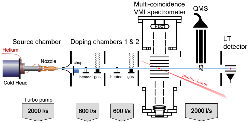
Figure 1: Experimental setup. A skimmed He droplet beam is produced from a cryogenically cooled continuous nozzle expansion with $5\text{\,}\mathrm{\SIUnitSymbolMicro m}$ diameter. The chopper wheel (‘chop.’) allows to alternatively measure foreground and background. Gas doping and oven cells enable pickup of dopants by the droplets. The droplets then cross the photon beam in the center of the spectrometer. A quadrupole mass spectrometer (QMS) and Langmuir-Taylor detector (LT) behind the spectrometer are used for beam diagnostics.

In this article we describe a new endstation that has recently been installed at the AMOLine of the ASTRID2 synchrotron at Aarhus University, Denmark Hertel and Hoffmann (2011). With this apparatus, our previous experiments at Elettra Buchta et al. (2013); LaForge et al. (2019) will be further extended owing to a more sophisticated imaging detector, extended doping capabilities, improved options for cluster beam characterization, and various cluster sources. We characterize the new PEPICO VMI spectrometer and present original data that illustrate the capability of the new setup to reveal the details of interatomic Coulombic decay (ICD) processes occurring in pure and doped He nanodroplets.Shcherbinin et al. (2017)

II Experimental setup

The new endstation placed at the end of the AMOLine of the ASTRID2 synchrotron is schematically shown in Fig. 1. A skimmed atomic, molecular or cluster beam traverses two vacuum chambers for doping with gas and oven cells before crossing the photon beam from the synchrotron in the center of an ion–electron coincidence spectrometer. The molecular or cluster beam then passes a chamber housing a quadrupole mass spectrometer (QMS) and is dumped in an additional small chamber, which is directly attached to the adjacent chamber without additional pumping. This beam dump also houses a simple Langmuir-Taylor (LT) detector for alkali and earth-alkali metals. Both chambers serve the purpose of monitoring the intensity and composition of the cluster beams. The pressure rise in the LT chamber in the presence of an He atomic or nanodroplet beam is on the order of ${10}^{-8}\text{\,}\mathrm{m}\mathrm{b}\mathrm{a}\mathrm{r}$.

For generating He nanodroplets we use a continuous cryogenic nozzle of diameter $5\text{\,}\mathrm{\SIUnitSymbolMicro m}$ placed at a distance of $12\text{\,}\mathrm{m}\mathrm{m}$ in front of a skimmer with $0.4\text{\,}\mathrm{m}\mathrm{m}$ diameter. Unless otherwise stated, all presented data were recorded with $30\text{\,}\mathrm{b}\mathrm{a}\mathrm{r}$ He backing pressure and $14\text{\,}\mathrm{K}$ nozzle temperature. The average number of He atoms per droplet was estimated by titration measurements Gomez et al. (2011) that yielded $\langle N_{\ch{He}}\rangle\approx 2000$. Typical operating pressures under these conditions are $1.4\text{\times}{10}^{-3}\text{\,}\mathrm{m}\mathrm{b}\mathrm{a}\mathrm{r}$ in the source, $4\text{\times}{10}^{-6}\text{\,}\mathrm{m}\mathrm{b}\mathrm{a}\mathrm{r}$ in the first and $6\text{\times}{10}^{-7}\text{\,}\mathrm{m}\mathrm{b}\mathrm{a}\mathrm{r}$ in the second doping chamber, $3\text{\times}{10}^{-8}\text{\,}\mathrm{m}\mathrm{b}\mathrm{a}\mathrm{r}$ in the VMI and QMS chambers and $5\text{\times}{10}^{-8}\text{\,}\mathrm{m}\mathrm{b}\mathrm{a}\mathrm{r}$ in the LT chamber.

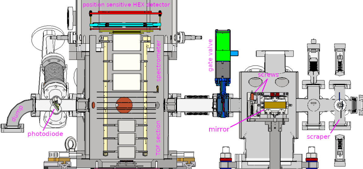
Figure 2: Spectrometer with beam dump and photodiode (left) and grazing incidence mirror and scrapers (right) for the incoming photon beam.

II.1 The AMOLine at ASTRID2

A cross-section of the spectrometer chamber and the adjacent mirror chamber to couple in the photon beam from the AMOLine is presented in Fig. 2. Two different gratings for the monochromator (not shown) provide 5 to $150\text{\,}\mathrm{e}\mathrm{V}$ photons from an undulator source on the ASTRID2 synchrotron. A slit and a selection of different foils can be used to adjust the photon intensity and suppress higher-order radiation. A focusing mirror after the monochromator is used to align the photon beam on the mirror (MC2) in Fig. 2 that refocuses the beam into the interaction region of the spectrometer (see Supporting Information S1). Several sets of scrapers placed upstream in the beamline are instrumental for reducing stray light reaching the mirror. The vertical position of the mirror is electronically controlled and can be replaced with either a photodiode or phosphor screen for photon beam diagnostics. The horizontal position (perpendicular to the beam direction) can be adjusted by movement of the chamber, while the pitch and yaw of the mirror are manually adjusted by a set of in-vacuum screws. The mirror chamber is separated from the spectrometer chamber by a pneumatic gate valve and a pinhole. The photon beam is dumped in a bent tube on the opposite side of the spectrometer which contains another phosphor screen and photodiode for beam diagnostics. Software integration of the data acquisition program and beamline control via TCP/IP allows several beamline parameters to be scanned for optimization, in particular the photon energy for automated photon-energy scans.

II.2 Beam source and doping options

A He atomic or nanodroplet beam is formed by a precooled continuous supersonic expansion through a $\mathrm{\SIUnitSymbolMicro m}$-size nozzle. The nozzle holder, body and He gas line are cooled by a closed-cycle cryostat that has a cooling power of $1\text{\,}\mathrm{W}$ at $4\text{\,}\mathrm{K}$. A copper heat shield mounted on the first cooling stage is not shown in Fig. 1. The nozzle temperature is continuously measured and regulated by resistive heating. Nozzle openings are formed by planar Pt foils (orifice diameters 5, 10 or $20\text{\,}\mathrm{\SIUnitSymbolMicro m}$) pressed into a copper holder. The open cylinder at the back of this holder is pressed onto a copper counterpart by a union nut and sealed with a C-shaped sealing ring. This facilitates the exchange of nozzles with different diameter. New nozzles are tested by measuring the He flow at $50\text{\,}\mathrm{b}\mathrm{a}\mathrm{r}$ backing pressure, which typically amounts to $1\text{\,}\mathrm{ml}\text{\,}{\mathrm{s}}^{-1}$ for a $5\text{\,}\mathrm{\SIUnitSymbolMicro m}$ nozzle. The supersonic expansion is skimmed to select the cold part of the beam before a shock wave is formed and for ensuring differential pumping. The skimmer holder is screwed into a threaded outer surface to adjust the nozzle-to-skimmer distance. The horizontal and vertical nozzle position can be varied by a translation stage without breaking vacuum.

To expand other gases, the same He nanodroplet source can be used where only the nozzle part has to be replaced by one with a larger diameter. Alternatively, it can be fully replaced by another beam source. A source for pure or molecule-doped water clusters based on the design of Förstel et al. Förstel et al. (2015) is currently in preparation.

In the oven chambers, four slots for heated ovens or gas doping cells enable sequential pickup of different dopants into He nanodroplets from solid, liquid or gaseous samples. This allows us to quickly apply different dopants or to form tailored multicomponent structures by adjusting the partial pressures and the order of doping the various substances into the droplet beam. The doping conditions are typically characterized by the QMS or by charge transfer ionization of dopants when irradiating the droplets with photons at energies $h\nu\geq E_{i}^{\ch{He}}$.

Figure 3: Spectrometer geometry. Half of the central cross-section of the electrode stack is depicted true to scale, including the center of the ionization region on the central axis. The inner electrodes are realized by metal plates with concentric holes. The outer ion stacks in Einzel lens configuration are realized by metal cylinders. The black bars on the far left and right specify the detector positions. The lengths of the VMI and TOF sections from the ionization region to the detectors are $247\text{\,}\mathrm{m}\mathrm{m}$ and $174\text{\,}\mathrm{m}\mathrm{m}$, respectively. Electrode positions and diameters are specified in Table 1.

Table 1: Electrode positions and inner radii of the spectrometer in Fig. 3.

Electrode	E6		E5		E4		E3		E2		E1		R1		R2		R3		R4		R5		R6		R7
Position/$\mathrm{m}\mathrm{m}$	-190.	625	-130.	875	-70.	625	-40.	0	-24.	0	-8.	0	8.	0	13.	0	24.	0	40.	0	62.	875	102.	875	142.	875
Radius/$\mathrm{m}\mathrm{m}$	42.	0	42.	0	42.	0	25.	0	20.	0	15.	0	7.	0	7.	0	11.	0	14.	0	25.	0	25.	0	25.	0

II.3 Spectrometer and VMI potentials

Two microchannel plate (MCP) detectors with a stack of $\mu$-metal shielded electrodes and a position-sensitive detection system, see Fig. 2, are currently set up to measure kinetic energies on one side and ion flight times for mass spectrometry on the other side of the spectrometer. Coincidence detection of cations and electrons allows us to obtain the ion time-of-flight (TOF) as the difference of electron and ion arrival times on the detectors. This detection mode is ideal for experiments with quasi-continuous photon beams as provided by synchrotrons.

The key strength of the electron and ion spectrometer is the combination of a RoentDek hexanode delay-line detector (HEX75) Jagutzki et al. (2002) with a set of electrodes to perform high-resolution VMI. The position-sensitive HEX75 detector is well suited for single particle detection at high event rates Österdahl et al. (2005) and in particular to reconstruct multi-hit events. In case of ion imaging, the $<$1\text{\,}\mathrm{n}\mathrm{s}$$ time resolution facilitates the full three-dimensional reconstruction of the momentum vectors of several ions in Coulomb explosion experiments Hasegawa, Hishikawa, and Yamanouchi (2001).

Fig. 3 shows a scaled drawing of the electrode configuration. The VMI section is similar to the spectrometer geometry at the GasPhase beamline at Elettra in Trieste, Italy O’Keeffe et al. (2011). A third extractor electrode is inserted and the flight tube is split into three tube sections to be used as an Einzel lens. The TOF and VMI sections of the spectrometer are separated by two meshes in the center that serve as repellers for VMI, labeled R1 and R2 in Fig. 3. The TOF section has a similar geometry with one electrode less, smaller electrode radius and shorter length. The time resolution does not noticeably depend on the specific electrode potentials, which are chosen to defocus the ions on the $40\text{\,}\mathrm{m}\mathrm{m}$ diameter MCP to reduce wear (see Figure 9). The combination of the MCP with a phosphor screen and digital camera allows us to monitor the spatial distribution of ions on the detector. When removing the central meshes, VMI could be performed on both sides of the spectrometer. The delay-line detector is combined with a larger $80\text{\,}\mathrm{m}\mathrm{m}$ diameter MCP which has the advantage of improved resolution when using higher VMI magnification and a larger maximum kinetic energy acceptance at a given magnification factor.

To achieve optimal VMI resolution it is crucial to optimize the potentials of the extractor electrodes to minimize the position spread due to the initial spatial distribution in the interaction region. The latter is defined by the overlap of the focused photon beam and the droplet beam, of which the extent in the horizontal plane is restricted to $4\text{\,}\mathrm{m}\mathrm{m}$ by a pair of adjustable scrapers. The three extractor electrodes and three electrodes in Einzel lens configuration are used to adjust the imaging properties to different ranges of electron kinetic energy. Trajectory simulations with the program SIMION Sim (2008) were used with a derivative based optimization routine Stei et al. (2013) to refine different sets of electrode potentials for optimal VMI conditions in a simple and quick way (see also Supporting Information S2). In the original method, derivatives are evaluated at zero initial kinetic energy. Here, the method was extended to nonzero values.

To calibrate the spectrometer in spatial map imaging mode, potassium-doped He nanodroplets were ionized with a Coherent Mira Ti:sapphire laser at continuous $767\text{\,}\mathrm{n}\mathrm{m}$ wavelength and about $0.56\text{\,}\mathrm{W}$ power. A lens with $175\text{\,}\mathrm{m}\mathrm{m}$ focal length was mounted on a translation stage to focus the light into the center of the interaction region. By shifting the focus position in the interaction region horizontally and vertically, we calibrated the positions on the detector and the ion time-of-flight, respectively Wituschek et al. (2016). Furthermore, a grating-stabilized diode laser is at our disposal to implement a simple scheme for photoionization of potassium atoms for precise calibration measurements Wituschek et al. (2016).

III Results and Discussion

III.1 Velocity mapping and resolution

Precise velocity map imaging is the basis for accurate measurements of electron or ion kinetic energy spectra and angular distributions. This section describes and characterizes different VMI potentials including scaled potentials to improve the resolution at low kinetic energies in the $\mathrm{e}\mathrm{V}$ range and use of Einzel lens electrodes to achieve detection up to kinetic energies of $100\text{\,}\mathrm{e}\mathrm{V}$.

III.1.1 Electron VMI without the Einzel lens

Spectrometer potentials for high resolution VMI imaging were determined with the numerical optimization routine. We refer to the Supporting Information for additional details (S2) and the obtained potentials (Table S.3). For calibration and characterization, a set of He+ images from photoionization in the gas phase is acquired at equally spaced photon energies, see Fig. 4. The energy calibration with empirical and simulation results in Fig. 5a and Table 2 is detailed in the Supporting Information (S3).

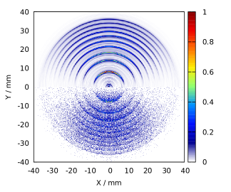
Figure 4: Photoelectron images for the ionization of gas-phase He at photon energies of 26, 29, 32, 35, 38, 41, 44, 47, 50 and $53\text{\,}\mathrm{e}\mathrm{V}$. Lower half: Raw images. Upper half: Abel inverted distributions.

The agreement of the near-linear calibration functions is very good with a maximum deviation of $0.9\text{\,}\mathrm{\char 37\relax}$ between simulation and measurement (black crosses in Fig. 5b). The higher-order coefficients $p_{1}$ and $p_{2}$ are not reproduced by the simulation. Their order of magnitude can be reproduced by a more detailed simulation taking into account an initial position distribution (see Supporting Information S4) that is offset from the center by $4\text{\,}\mathrm{m}\mathrm{m}$ away from the detector and $9\text{\,}\mathrm{m}\mathrm{m}$ along the photon beam (last row in Table 2). Besides imperfect centering of the photon beam and the He beam, also small deviations from the ideal electrical field and residual magnetic fields may contribute to the nonlinearities.

Table 2: Calibration coefficients for VMI without Einzel lens. The calibration function is $E_{\mathrm{kin}}=p_{0}R^{2}+p_{1}R^{4}+p_{2}R^{6}$. Uncertainties in parentheses are given in units of the last digit.

Origin	$p_{0}$	$p_{1}/\text{\small${10}^{-7}$}$	$p_{2}/\text{\small${10}^{-9}$}$
Experiment	$0.0235(1)$	$21(3)$	$-1.5(1)$
Simulation	$0.023\,58$	$1.13(2)$	$0.0013(8)$
with offset	$0.0260(4)$	$26(11)$	$-1.5(10)$

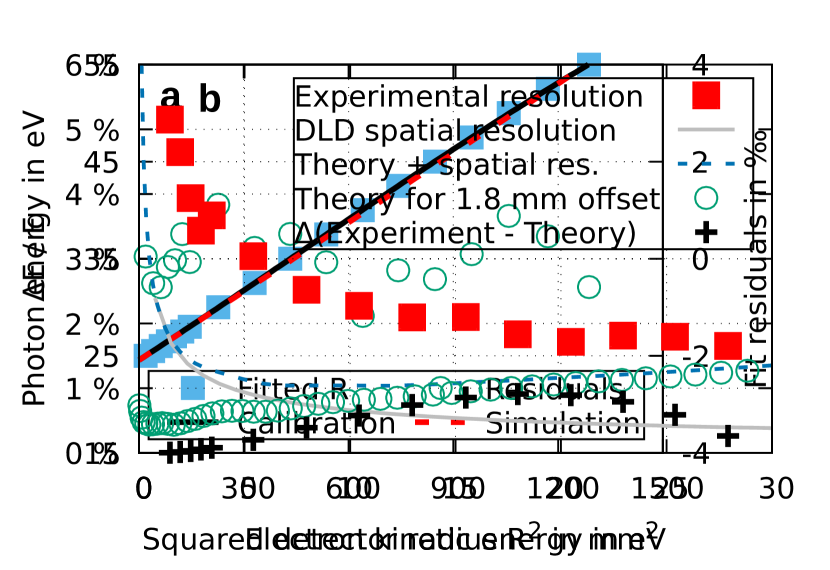
Figure 5: Results of a calibration measurement in comparison with simulation results. (a) Photon energy as a function of the squared detector radius with a polynomial fit. (b) Experimental energy resolution, simulated deviations due to off-center start positions and relative deviation between the simulated and the empiric calibration function.

III.1.2 Energy resolution limits

Quantifying the energy resolution by the ratio of the standard deviation $\Delta E$ to the magnitude of the electron kinetic energy $E$, the VMI settings without Einzel lens perform best with $\Delta E/E=$1.7\text{\,}\mathrm{\char 37\relax}$$ at large detector radii. The resolution stays below $2.1\text{\,}\mathrm{\char 37\relax}$ down to about $13\text{\,}\mathrm{e}\mathrm{V}$ kinetic energy in Fig. 5b. Below $13\text{\,}\mathrm{e}\mathrm{V}$, the absolute radial spread stays constant near $230\text{\,}\mathrm{\SIUnitSymbolMicro m}$ so the energy resolution decreases and reaches $5\text{\,}\mathrm{\char 37\relax}$ at $1.5\text{\,}\mathrm{e}\mathrm{V}$ kinetic energy.

A position resolution of $160\text{\,}\mathrm{\SIUnitSymbolMicro m}$ Österdahl et al. (2005) FWHM and better can be achieved with the HEX75 detector for atoms and ions, corresponding to a standard deviation of $68\text{\,}\mathrm{\SIUnitSymbolMicro m}$. Electrons produce signal amplitudes with lower magnitude and higher variance and we expect a resolution limit of $100\text{\,}\mathrm{\SIUnitSymbolMicro m}$ represented by the gray line in Fig. 5b. The simulated energy broadening (see details in Supporting Information S4) due to the initial spatial distribution in the interaction region (green circles) only slightly raises this resolution limit (blue dashed line) that stays more than a factor $2$ below the experimental resolution. One possible explanation is the so far not controlled vertical position of the photon beam: The assumption of a $4\text{\,}\mathrm{m}\mathrm{m}$ offset from center irrespectively of the direction mostly reproduces the experimental result (blue triangles). The horizontal position has a minor effect on the simulated resolution. A later improvement of the detector resolution with higher MCP gain did not result into a better experimental resolution which supports the hypothesis that ajdustment of the interplay between vertical position and electrode potentials may further improve the achieved energy resolution.

Alternative potentials with improved resolution for low and high electron kinetic energy ranges are presented in the following.

III.1.3 Alternative VMI potentials

The maximum kinetic energy acceptance with $-3.5\text{\,}\mathrm{k}\mathrm{V}$ extraction potential without using the Einzel lens is about $32\text{\,}\mathrm{e}\mathrm{V}$. In highly excited or core ionized systems, it is often desirable to capture faster electrons to probe the process of interest or to include photoelectrons from direct ionization as a reference, e.g. to determine branching ratios.

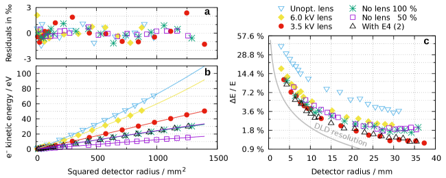
Figure 6: Fit residuals (a), calibration fits (b) and energy resolution (c) for different VMI settings. The corresponding electrode potentials are specified in Table S.3. The gray line indicates the expected resolution limit of the HEX75 detector for electrons.

We have achieved compression of electron VMI images with identical positive potentials on the outer electrodes E4, E6 of the Einzel lens and refer to the Supporting Information (S2) for additional explanations. The calibration curves in Fig. 6b visualize the resulting energy acceptance. There is no empirical data above $70\text{\,}\mathrm{e}\mathrm{V}$ kinetic energy as the high energy grating for the monochromator was not available when the data were taken.

Simply adding $6\text{\,}\mathrm{k}\mathrm{V}$ potentials to the optimized potentials without the lens gives the highest energy acceptance up to $100\text{\,}\mathrm{e}\mathrm{V}$ but significantly decreases the energy resolution, see Fig. 6c (”Unopt. lens”, blue triangles). Numerical re-optimization for VMI conditions almost restores the original energy resolution (yellow diamonds) at the cost of somewhat lower $90\text{\,}\mathrm{e}\mathrm{V}$ maximum energy.

Optimized potentials with a $3.5\text{\,}\mathrm{k}\mathrm{V}$ Einzel lens are a good compromise with $50\text{\,}\mathrm{e}\mathrm{V}$ energy acceptance and excellent resolution reaching down to $1.2\text{\,}\mathrm{\char 37\relax}$ in the high-energy range.

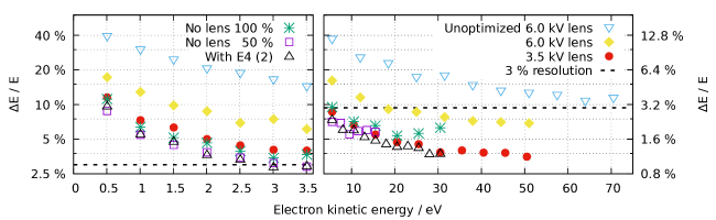
Figure 7: Energy resolution as a function of electron kinetic energy for different VMI settings. The corresponding electrode potentials are specified in Table S.3. The $6\text{\,}\mathrm{k}\mathrm{V}$ Einzel lens settings are applicable up to $90\text{\,}\mathrm{e}\mathrm{V}$ and above (see Fig. 6b) which has not been recorded. The $x$ range is split in two parts with different $y$ ranges. Dashed lines at $3\text{\,}\mathrm{\char 37\relax}$ resolution are shown to guide the eye.

The energy resolution decreases quickly at low energies in the $1\text{\,}\mathrm{e}\mathrm{V}$ range and this would still be true if the spatial resolution limit of the detector (gray line) could be reached. Therefore, a larger velocity magnification factor is required to significantly improve the resolution for slow electrons. This can to some extent be achieved by scaling the extraction potentials and is demonstrated for the settings without an Einzel lens scaled to $100\text{\,}\mathrm{\char 37\relax}$ (stars) and $50\text{\,}\mathrm{\char 37\relax}$ (squares) of the full potentials. While the resolution as a function of radius cannot be substantially altered (Fig. 6c), the resolution at a specific energy is improved. This becomes evident in Fig. 7, which summarizes all settings with the resolution as a function of kinetic energy. The $50\text{\,}\mathrm{\char 37\relax}$ results demonstrate the limits of this approach: scaling the potentials by a factor of $2$ improved the resolution by merely $15\text{\,}\mathrm{\char 37\relax}$ and settings below $30\text{\,}\mathrm{\char 37\relax}$ potentials were empirically found to be inadequate for imaging.

The $100\text{\,}\mathrm{\char 37\relax}$ potentials can be further improved by using lens E4 while the other two electrodes of the Einzel lens are kept at ground potential. Settings optimized for $30\text{\,}\mathrm{e}\mathrm{V}$ kinetic energy (see Supporting Information Table S.3) reach the resolution of the $50\text{\,}\mathrm{\char 37\relax}$ potentials without compromising the kinetic energy acceptance in Fig. 7. The disadvantage is a significantly reduced time-of-flight resolution due to a shallower extraction potential (”low res.” in Fig. 10).

Another elegant approach for low kinetic energies is to use a short Einzel lens in the flight tube to magnify the spatial distribution by inversion Offerhaus et al. (2001). Ramping up the lens first focuses electrons of different kinetic energy until reaching inversion and then starts magnifying the inverted electron image. To be efficient, this approach requires a shorter Einzel lens with smaller diameter than in our spectrometer geometry. The original geometry would thus limit the spectrometer to relatively low kinetic energies. Furthermore, such a geometry reduces the VMI quality with a significant dependence on the initial particle position in a way that cannot be compensated for by the numerical optimization routine. A more detailed analysis will be required to evaluate the trade-off between the different sources of uncertainty.

III.2 Spatial mapping and beam overlap

III.2.1 SMI potentials and calibration

In analogy to VMI but with inverse logic, the spectrometer can be used for spatial map imaging (SMI) in the interaction region with high precision, irrespectively of the initial velocities of the imaged particles.Stei et al. (2013) We have employed two-dimensional SMI for calibration and to characterize the overlap of the photon and He beam in the scattering plane. The numerical optimization routine was employed to determine potentials for three different settings that are presented in the Supporting Information (S5): (1) two-dimensional SMI of radial positions, (2) magnified two-dimensional SMI and (3) one-dimensional TOF-SMI of axial positions.

Calibration measurements for SMI settings were performed by ionizing potassium doped HNDs at $767\text{\,}\mathrm{n}\mathrm{m}$ wavelength. The magnification factor for ion or electron SMI was found to be $-3.2$, in excellent agreement with the simulation value $-3.154$ ($1.5\text{\,}\mathrm{\char 37\relax}$ deviation). With the magnifying settings, a factor of $-13$ was found ($3\text{\,}\mathrm{\char 37\relax}$ deviation) and the TOF-SMI has a scaling factor of $64\text{\,}\mathrm{ns}\text{\,}{\mathrm{mm}}^{-1}$ ($10\text{\,}\mathrm{\char 37\relax}$ deviation).

III.2.2 SMI resolution

Cation SMI with K+ ions gives an upper bound standard deviation of $50\text{\,}\mathrm{\SIUnitSymbolMicro m}$ for the waist of the focused beam (see Supporting Information, Table S.6). This corresponds to a radius of $160\text{\,}\mathrm{\SIUnitSymbolMicro m}$ on the detector, larger than the expected spatial resolution of the HEX75 detector of about $70\text{\,}\mathrm{\SIUnitSymbolMicro m}$ or lower. The same width is observed for the magnifying settings, which however corresponds to $670\text{\,}\mathrm{\SIUnitSymbolMicro m}$ on the detector. We assume that this is caused by stronger velocity broadening in line with the simulations that predict a significant derivative of the impact position with respect to the initial ion velocity, see Supporting Information (S5). The TOF-SMI settings give a similar value of $50\text{\,}\mathrm{\SIUnitSymbolMicro m}$ for the vertical direction which corresponds to a standard deviation of $3\text{\,}\mathrm{n}\mathrm{s}$ in the ion flight times which is larger than the optimum time resolution of the HEX75 detector of about $0.5\text{\,}\mathrm{n}\mathrm{s}$.

With electron SMI at full and $50\text{\,}\mathrm{\char 37\relax}$ potentials (scaling $s=1$ and $0.5$), the standard deviations are $w=$80\text{\,}\mathrm{\SIUnitSymbolMicro m}$$ and $110\text{\,}\mathrm{\SIUnitSymbolMicro m}$. The simplified assumption $w=w_{0}+c/\sqrt{s}$ with beam waist $w_{0}$ and velocity dependent broadening thus gives the estimate $w_{0}\approx$7.6\text{\,}\mathrm{\SIUnitSymbolMicro m}$$. The order of magnitude is confirmed by the $8.5\text{\,}\mathrm{\SIUnitSymbolMicro m}$ focused spot radius of a Gaussian beam with $5\text{\,}\mathrm{m}\mathrm{m}$ radius at the focusing lens. The experimental conditions are therefore suited to assess the resolution of about $50\text{\,}\mathrm{\SIUnitSymbolMicro m}$ (RMS) for ions that is achieved with the SMI mode.

III.2.3 Width of the He droplet beam

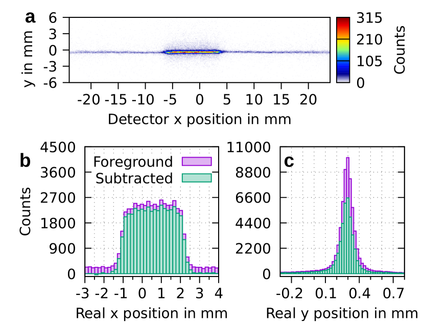
Figure 8: Cation spatial map image (a), and its projections on the He beam (b) and photon beam (c) axis. A HND beam at $30\text{\,}\mathrm{b}\mathrm{a}\mathrm{r}$ backing pressure and $12\text{\,}\mathrm{K}$ nozzle temperature is ionized by $25\text{\,}\mathrm{e}\mathrm{V}$ photons. Ionization of the background gas makes the photon beam visible and is subtracted from the projections to show the droplet related contribution. The conversion to real position is detailed in Supporting Information S5.

For a cold HND beam ionized at the synchrotron at $25\text{\,}\mathrm{e}\mathrm{V}$ photon energy, the raw SMI image on the detector and the centered projections in units of real length are shown in Fig. 8. The presented data are not mass selected, such that the photon beam is clearly visible from ionized background gas. The measurements were performed with a running chopper wheel. The rising and falling edges of a TTL monitor signal were acquired with the TDC to filter foreground and background events in the data analysis. Fig. 8b demonstrates the clear isolation of the droplet related signal by subtraction. The full width of the droplet beam profile at the baseline is $4.3\text{\,}\mathrm{m}\mathrm{m}$, close to the $4\text{\,}\mathrm{m}\mathrm{m}$ width of the scrapers that limit the horizontal extension of the droplet beam. The FWHM of a Gaussian fit to the photon beam profile is $0.12\text{\,}\mathrm{m}\mathrm{m}$ in good agreement with an estimate of $0.11\text{\,}\mathrm{m}\mathrm{m}$ derived from ray-tracing results in the Supporting Information (S1).

III.3 Time-of-flight mass spectrometry

Currently two meshes separate the VMI section from the TOF section which impedes to use the latter for velocity mapping. In principle, the TOF section can be used to collect electrons that define a zero point in arrival time to perform mass selective cation imaging in continuous beam experiments. In case of electron imaging, the TOF section provides complimentary information on the mass of coincident cations which is a powerful tool to probe if different ion formation channels involve different electronic states.

It has been found that the specific potentials of the electrodes in the TOF section (see Fig. 3) have only a small effect on the time resolution. Therefore, the potentials can be chosen to defocus the ions to increase the detector lifetime. This is demonstrated by an integrated intensity image of the phosphor screen in Fig. 9.

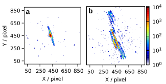
Figure 9: Defocusing ions on the TOF detector. Electrode potentials are E1: $-1433.5\text{\,}\mathrm{V}$, R1/R2: $-1750\text{\,}\mathrm{V}$, R5/R7: $-3550\text{\,}\mathrm{V}$ and R6: $-4250\text{\,}\mathrm{V}$. The MCP front and R6 potentials are the same. (a) Focused ions with $\mathrm{R3}=\mathrm{R2}$ and $\mathrm{R4}=\mathrm{R5}$. (b) Defocused ions with $\mathrm{R3}=\mathrm{R4}=$-3000\text{\,}\mathrm{V}$$.

Two example mass spectra are presented in Fig. 10. The first shows a progression of clusters from a pure He beam. The droplets were ionized at $67.5\text{\,}\mathrm{e}\mathrm{V}$ above the first excited level of He+. Some He_n^+ peaks are mixed with water, nitrogen, oxygen and carbon dioxide and their fragments from the background gas in the VMI chamber that also contains He+ from effusive He. Double electron coincidences from direct ionization and subsequent ICD at this photon energy are presented below.

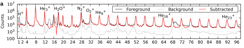
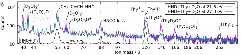
Figure 10: Mass spectra of (a) pure HNDs ($h\nu=$67.5\text{\,}\mathrm{e}\mathrm{V}$$) and (b) HNDs doped with thymine and D2O where dopants are Penning ionized ($21.6\text{\,}\mathrm{e}\mathrm{V}$) and charge-transfer ionized ($27\text{\,}\mathrm{e}\mathrm{V}$). Acquisition times were about $20\text{\,}\mathrm{h}$ ($21.6\text{\,}\mathrm{e}\mathrm{V}$) and $6.5\text{\,}\mathrm{h}$ ($27\text{\,}\mathrm{e}\mathrm{V}$) and the data of the latter are scaled by a factor of 0.3. The mass spectra in (b) are background subtracted. The solid black line shows a mass spectrum without D2O and with reduced TOF resolution at $21.6\text{\,}\mathrm{e}\mathrm{V}$ photon energy.

The second mass spectrum shows the mass resolution achieved with the $100\text{\,}\mathrm{\char 37\relax}$ VMI settings without using the Einzel lens electrodes. For these data, HNDs were doped with the nucleobase thymine (oven heated to $100\text{\,}\mathrm{\SIUnitSymbolCelsius}$, $\sim$ $9.6\text{\times}{10}^{-6}\text{\,}\mathrm{m}\mathrm{b}\mathrm{a}\mathrm{r}$ vapor pressure Ferro et al. (1980)) and deuterated water ($3.3\text{\times}{10}^{-6}\text{\,}\mathrm{m}\mathrm{b}\mathrm{a}\mathrm{r}$ partial pressure leaked directly into the vacuum chamber). The nucleobase was ionized and fragmented by either Penning ionization from He excited at a photon energy $h\nu=$21.6\text{\,}\mathrm{e}\mathrm{V}$$ or by charge transfer to He ionized at $h\nu=$27\text{\,}\mathrm{e}\mathrm{V}$$. Single mass peaks are resolved up to around $40\text{\,}\mathrm{u}$, still clearly visible around $80\text{\,}\mathrm{u}$ and start to convolute around $120\text{\,}\mathrm{u}$. This allows us to identify several thymine fragments with different hydrogen content and mixed clusters with up to $4$ attached heavy water molecules. Also pure water clusters up to $n=3$ are seen. The protonated water complex (D2O)_3D+ is indicative for the presence of larger clusters. Charge transfer leads to stronger fragmentation of thymine-D2O complexes and thymine clusters, whereas in the case of Penning ionization, larger clusters and thymine dimers are present in the spectrum.

III.4 Energy scan of a Fano resonance

Double excitation into the He 2s2p state at $h\nu=$60.15\text{\,}\mathrm{e}\mathrm{V}$$ gives rise to an atomic Fano resonance that is broadened and shifted to around $60.4\text{\,}\mathrm{e}\mathrm{V}$ in He nanodroplets LaForge et al. (2016). The autoionization of a doubly excited atom can compete with the ionization of a neighbor atom. The second process is called Interatomic Coulombic Decay (ICD) and results into a lower electron kinetic energy (eKE). This has been theoretically shown for HeNe dimers, where ICD is increasingly competitive with excitation into higher Rydberg orbitals Jabbari, Gokhberg, and Cederbaum (2020). Unfortunately, investigating ICD between neighboring He atoms in HNDs is complicated by inelastic scattering of the photoelectron Shcherbinin et al. (2019) giving rise to the same eKE if the same singly excited state is involved, e.g. 1s2p. The inelastic scattering rate is expected to follow the Fano line shape of the photoline. In that case the ratio between low and high eKE would remain constant. If, however, ICD contributed to the electron yield, we would expect a pronounced increase of this ratio at the double excitation resonance.

We therefore performed detailed photon energy scans around the $60.4\text{\,}\mathrm{e}\mathrm{V}$ and higher resonances that will be presented in a separate publication. The VMI potentials with a $3.5\text{\,}\mathrm{k}\mathrm{V}$ Einzel lens were ideally suited for these measurements, providing excellent resolution and a wide electron kinetic energy range including photoelectrons (see Fig. 7). Fig. 11 shows an example of two electron images recorded in coincidence with He+ and He2+ and the total eKE distributions at different photon energies. The photoline originates from direct ionization and autoionization while the 1s2p peak is due to ICD or inelastic scattering. We can thus compare relative rates as a function of selected electron/ion coincidences, electron kinetic energy and photon energy.

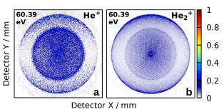
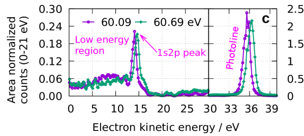
Figure 11: Electron images in coincidence with (a) He+ and (b) He2+ ions and (c) total eKE distributions at different photon energies around the 2s2p HND resonance ($30\text{\,}\mathrm{b}\mathrm{a}\mathrm{r}$ backing pressure, $14\text{\,}\mathrm{K}$ nozzle). The He+ coincidence image and total eKE spectra are background subtracted.

The He+ coincidence image in Fig. 11a is background subtracted to remove the contribution of background He to the photoline (the He2+ image is background free). In general, the background-subtraction factor is corrected as described in the Supporting Information (S6). To obtain energy distributions, foreground and background images are inverted separately using MEVELER to avoid pixel noise and to fulfill the requirement of Poissonian statistics Dick (2014).

The electron images additionally contain angular information. Distributions of the angle $\theta$ between the photoelectron velocity vector and the polarization axis at $60.39\text{\,}\mathrm{e}\mathrm{V}$ photon energy are presented in Fig. 12 with fit results for the anisotropy parameter $\beta$. The background-subtracted droplet contribution from the photoline in coincidence with He+ slightly deviates from the nearly perfect $\cos^{2}\theta$ dependence as measured for background He atoms. This indicates a deflection of the emitted electrons presumably by elastic scattering of the electrons at He atoms. The He2+ photoline has a strong isotropic contribution and the low-kinetic-energy electrons ($<$22\text{\,}\mathrm{e}\mathrm{V}$$ in Fig. 11) are predominantly isotropic due to massive elastic and inelastic electron-He scattering. A detailed analysis of the electron angular distributions of He nanodroplets will be presented elsewhere.

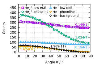
Figure 12: Angle distributions at $60.39\text{\,}\mathrm{e}\mathrm{V}$ photon energy. Solid lines are $1+\frac{\beta}{2}\left(3\cos^{2}\theta-1\right)$ fits. Resulting $\beta$-values are shown in the same color. The curve for the He+ photoline is background subtracted.

The narrow lineshape of the atomic 2s2p Fano resonance allows us to determine the energy resolution of the photon beam in the given energy range. To this end, we convolute the Fano line shape Kossmann, Krassig, and Schmidt (1988) with a Gaussian function as described by Domke et al. Domke et al. (1996) The standard deviation of the Gaussian is determined by a least-squares fit, see Fig. 13. The energy resolution depends on the width of the monochromator exit slit. Measurements are usually taken with $150\text{\,}\mathrm{\SIUnitSymbolMicro m}$ exit-slit width corresponding to an absolute photon energy resolution of $14\text{\,}\mathrm{m}\mathrm{e}\mathrm{V}$ or a resolving power of 4300. By further reducing the slit width to $100\text{\,}\mathrm{\SIUnitSymbolMicro m}$ the resolution can be further improved to $10\text{\,}\mathrm{m}\mathrm{e}\mathrm{V}$, at the cost of reduced photon flux, though. The measurement of the atomic Fano resonance position is also used for absolute energy calibration of the beamline.

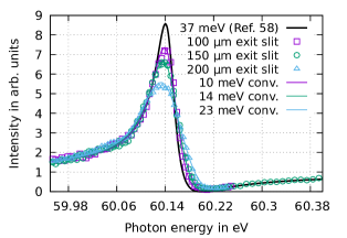
Figure 13: Least-squares fits to an atomic Fano resonance for different monochromator exit slit widths. Gaussian functions with the specified widths are convoluted with the Fano profile (black curve) with parameters by Domke et al. Domke et al. (1996)

III.5 Coincidences and multi-hits

Owing to the multi-hit capability of the HEX75 detector, it is possible to record two electrons from the same ionization event. By identifying coincidences both between electrons and between ions and electrons, we can select specific ionization processes in the analysis. To demonstrate the capability of this detection scheme, we revisit a previous experiment done at the GasPhase beamline at Elettra Shcherbinin et al. (2017). There, we studied Interatomic Coulombic Decay (ICD) in pure He nanodroplets upon formation of an excited He ion through the shake-up process.

$$\ch{He}-\ch{He}\xrightarrow{h\nu}\ch{He^{+*}}+\ch{He}+\ch{e_{sat}-}\\ \xrightarrow{\text{ICD}}\ch{He+}+\ch{He+}+\ch{e_{sat}-}+\ch{e_{ICD}-}$$ (1)

The total number of charged particles from the process is then 4 (two electrons and two cations). In our previous study of this process, detection of two ions with different masses in coincidence with a single electron was possible, but detection of multi-hits of electrons was impossible; only a single electron was measured for each ionization event. With our new endstation, detection of all products of the ICD process is now possible. Furthermore, with our optimized VMI settings using the Einzel lens (see section III.1.3), we can image the electrons from direct photoionization ($E_{\text{kin}}=h\nu-E_{i}^{\ch{He}}$) as well as the satellite photoelectron (e_sat-) from shake-up ionization and the ICD electron (e_ICD-).

Figure 14 displays coincidences between two ions recorded at $67.5\text{\,}\mathrm{e}\mathrm{V}$. Detection of two ions with identical mass-to-charge ratio is impossible for the current use of the ion detector because they have nearly equal flight times and thus one ion arrives within the deadtime of the detector caused by the other ion. The most abundant ion-ion coincidence is the ion pair He+/He2+. Simultaneously detected two He_$k$+ ions stem from either ICD or impact ionization following direct photoionization. The different ionization processes can be identified by inspecting the electron kinetic energy spectra. Figure 15 displays electron spectra for various cuts on the coincidence data recorded at $67.5\text{\,}\mathrm{e}\mathrm{V}$. From the coincidences of a single electron with either the He+ or He2+ ion, we can identify four peaks in the spectra. The peak at $\sim$43\text{\,}\mathrm{e}\mathrm{V}$$ is due to photoelectrons emitted by direct photoionization, whereas the peak at $\sim$22\text{\,}\mathrm{e}\mathrm{V}$$ is due to inelastic scattering of the photoelectron with another He atom in the droplet Shcherbinin et al. (2019). In the case of direct photoionization in coincidence with He+, the photoline stems from the component of free atoms accompanying the droplet beam.Shcherbinin et al. (2019) The sharp line at $2.2\text{\,}\mathrm{e}\mathrm{V}$ corresponds to satellite electrons, e_sat-, and the broad feature centered around $8\text{\,}\mathrm{e}\mathrm{V}$ are ICD electrons, e_ICD-.

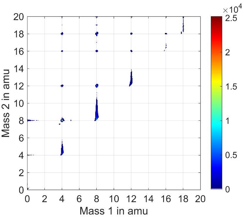
Figure 14: Background-subtracted electron/ion/ion coincidence time-of-flight mass spectrum recorded at $67.5\text{\,}\mathrm{e}\mathrm{V}$ photon energy, $30\text{\,}\mathrm{b}\mathrm{a}\mathrm{r}$ backing pressure and $14\text{\,}\mathrm{K}$ nozzle temperature.

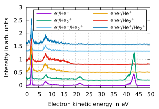
Figure 15: Electron kinetic energy distribution for different coincidences recorded at $67.5\text{\,}\mathrm{e}\mathrm{V}$ photon energy (nozzle at $14\text{\,}\mathrm{K}$ and $30\text{\,}\mathrm{b}\mathrm{a}\mathrm{r}$). In the case of coincidences involving two electrons, the spectrum contains the sum of the two electrons.

Direct photoionization and inelastic electron-He scattering leading to He excitation are processes creating only a single electron/cation pair. Therefore, the two peaks from these processes are suppressed in the electron spectra for coincidences of more than one electron and/or ion. The e_sat- and e_ICD- electrons are present in the spectra for all shown coincidence schemes, which shows that by selecting a certain coincidence scheme, we can filter for a specific ionization channel — in this case ICD. The two electrons from the ICD process arrive at the detector nearly at the same time such that we cannot separate them into two images. Instead, the spectra for coincidences of two electrons with one or two ions show the sum of the two electrons from each event. Setting the condition that the two electrons arrive at the detector simultaneously ($\Delta t<$10\text{\,}\mathrm{n}\mathrm{s}$$) helps to significantly suppress false coincidences. Differences in the shape of the ICD feature are seen depending on whether the coincidence cut includes the He+ ion or only the He2+ ion. In triple e-/e-/He2+ coincidences, the ICD feature extends to higher kinetic energy compared to the ICD feature for e-/e-/He+ coincidences. ICD between two He atoms at a larger interatomic distance leads to an increased kinetic energy of the electron in connection with a decreased kinetic energy release of the ions from Coulomb explosion Sisourat et al. (2010). Thus, the high kinetic energy part in the ICD electron peak for e-/e-/He2+ coincidences is due to ICD between two He atoms at large interatomic distance, which after ionization are more likely to pick up other He atoms before leaving the droplet due to their reduced kinetic energy. Consequently, the detection of this high-energy part of the ICD feature is suppressed for e-/e-/He+ coincidences.

As already mentioned, electron impact ionization following direct photoionization can also lead to two electron/cation-pairs. The characteristic feature for impact ionization would be a broad feature reaching from zero kinetic energy to the excess energy following impact ionization ($h\nu-2E_{i}^{\ch{He}}=$18.3\text{\,}\mathrm{e}\mathrm{V}$$) due to uniformly distributed energy sharing between the two electrons Shcherbinin et al. (2019). This is clearly seen in the e-/e-/He2+ coincidences in agreement with the formation of He2+ after the creation of a slow ion by electron impact. In most other channels, a clear minimum of zero intensity is present between the e_sat- and e_ICD- peaks, so we conclude a minor importance of impact ionization.

From the detection of either a single electron or the two electrons from the ICD process, we can estimate the detection efficiency of electrons on the HEX75 detector using the following formulas

$$f_{1} =df_{\text{tot}}-f_{2},$$ (2)

$$f_{2} =d^{2}f_{\text{tot}},$$ (3)

where $f_{1,\,2}$ is the rate of detecting either one or two electrons per ICD event, $f_{\text{tot}}$ is the real ICD event rate and $d$ is the detection efficiency of each electron. The yields ($I_{1,\,2}$) of ICD electrons from observed one or two electron coincidences are then

$$I_{1} =f_{1}t,$$ (4)

$$I_{2} =2f_{2}t,$$ (5)

where $t$ is the measurement time, and the factor 2 comes from the fact that electron spectra for coincidences of two electrons contain the sum of both electrons. From the ICD-related yield of coincidences including either a single electron or both electrons, we then determine the detection efficiency to be $\sim$20\text{\,}\mathrm{\char 37\relax}$$. From the $>$$70\text{\,}\mathrm{\char 37\relax}$ open area ratio (OAR) of the MCPs, we would expect $\sim$30\text{\,}\mathrm{\char 37\relax}$$ loss of electrons at the MCPs Fehre et al. (2018). Further loss of electrons happens at the mesh in front of the detector, and due to dependencies of the detection efficiency on the kinetic energy of the electrons Müller et al. (1986).

III.6 Detection of anions

Identification of ions by their time-of-flight in continuous experiments relies on coincidence detection. The simplest case is photoionization, as the electron flight time is negligible for mass spectrometry of the cations. Anion detection is of interest for example to study electron attachment processes.Fabrikant et al. (2017) In He nanodroplets, electrons with relevant kinetic energies can be created by photoionization. After subsequent resonant Jaksch et al. (2009) or dissociative da Silva et al. (2009) electron attachment, the formed anion will be detected in coincidence with the photoionized cation.

As a proof of concept for anion detection, we probed resonant $\ch{O2}+h\nu\rightarrow\ch{O+}+\ch{O-}$ pair formation at $17.47\text{\,}\mathrm{e}\mathrm{V}$ photon energy Dehmer and Chupka (1975); Zhou and Mo (2013). The cation flight time can be directly measured with photon energies above the appearance energy of O+. In case of pair formation, the event is triggered by O- on the HEX75 detector and due to the longer flight time of the anion, the O+ is observed at negative arrival time. The flight time of the coincident cation plus the negative arrival time axis thus gives the anion TOF spectrum and allows to set a cut on the O- image that is shown in Fig. 16.

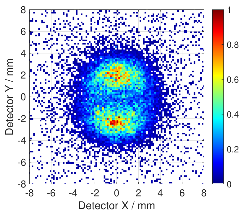
Figure 16: Ion images of O- ions detected in coincidence with O+ following ion pair formation from O2 at $h\nu=$17.47\text{\,}\mathrm{e}\mathrm{V}$$.

In such measurements of anion–cation coincidences, the primary photoelectrons should be suppressed. For this purpose we have added a simple construction to insert strong magnets near the ionization region. While leaving the anion TOF and image unperturbed, the electron count rate was reduced by half. We expect to improve the suppression of electrons by adding a second magnet tube on the opposite side.

IV Conclusion and outlook

In summary, we have described in detail a new endstation that complements the experimental capabilities of the AMOLine of the ASTRID2 synchrotron radiation facility. Using pure and doped He nanodroplets that were resonantly excited or ionized by XUV radiation, we characterized the performance of the imaging spectrometer with regard to high-resolution VMI photoelectron spectra, ion time-of-flight mass spectra, and spatial mapping of the ionization region. The capability of detecting electrons and ions in coincidence up to e-/e-/ion/ion quadruple coincidences was demonstrated. Original multi-coincidence ICD electron spectra in the regimes of He-droplet double excitation and shake-up ionization were discussed. Furthermore, we presented measurements of oxygen anion/cation coincidences, electron angular distributions of pure He nanodroplets, and fragment-ion mass spectra of thymine-D2O complexes formed in He nanodroplets doped with thymine and water.

This endstation will be continuously upgraded in the following directions: A continuous cluster source for producing heavier rare-gas clusters and water clusters mixed with biomolecules is in preparation. The addition of an aerosol injector is planned. Simultaneous imaging of electrons and ions in a double imaging geometry Bodi et al. (2012); Garcia et al. (2013) is envisioned. The implementation of a IR-UV fluorescence spectrometer will further widen the scope of future experimental studies.

Author declarations

The authors have no conflicts to disclose.

Data Availability Statement

The data that support the findings of this study are available from the corresponding author upon reasonable request.

References

- Han et al. (2018) P. Han, W. Martens, E. R. Waclawik, S. Sarina, and H. Zhu, Particle & Particle Systems Characterization 35, 1700489 (2018).
- Liz-Marzán, Murphy, and Wang (2014) L. M. Liz-Marzán, C. J. Murphy, and J. Wang, Chem. Soc. Rev. 43, 3820 (2014).
- Wang, Friedlander, and Mädler (2005) C. Wang, S. K. Friedlander, and L. Mädler, China Particuology 3, 243 (2005).
- Butterworth et al. (2012) K. T. Butterworth, S. J. McMahon, F. J. Currell, and K. M. Prise, Nanoscale 4, 4830 (2012).
- Eppink and Parker (1997) A. T. J. B. Eppink and D. H. Parker, Rev. Sci. Instrum. 68, 3477 (1997).
- Garcia et al. (2005) G. A. Garcia, L. Nahon, C. J. Harding, E. A. Mikajlo, and I. Powis, Rev. Sci. Instrum. 76, 053302 (2005).
- Hosaka et al. (2006) K. Hosaka, J. Adachi, A. V. Golovin, M. Takahashi, N. Watanabe, and A. Yagishita, Jpn. J. Appl. Phys. 45, 1841 (2006).
- Rolles et al. (2007) D. Rolles, Z. Pešić, M. Perri, R. Bilodeau, G. Ackerman, B. Rude, A. Kilcoyne, J. Bozek, and N. Berrah, Nucl. Instrum. Meth. B 261, 170 (2007).
- Tang et al. (2009) X. Tang, X. Zhou, M. Niu, S. Liu, J. Sun, X. Shan, F. Liu, and L. Sheng, Rev. Sci. Instrum. 80, 113101 (2009).
- O’Keeffe et al. (2011) P. O’Keeffe, P. Bolognesi, M. Coreno, A. Moise, R. Richter, G. Cautero, L. Stebel, R. Sergo, L. Pravica, Y. Ovcharenko, et al., Rev. Sci. Instrum. 82, 033109 (2011).
- Garcia et al. (2013) G. Garcia, B. Cunha de Miranda, M. Tia, S. Daly, and L. Nahon, Rev. Sci. Instrum. 84, 053112 (2013).
- Bodi et al. (2012) A. Bodi, P. Hemberger, T. Gerber, and B. Sztáray, Rev. Sci. Instrum. 83, 083105 (2012).
- Tang et al. (2015) X. Tang, G. A. Garcia, J.-F. Gil, and L. Nahon, Rev. Sci. Instrum. 86, 123108 (2015).
- Kostko et al. (2017) O. Kostko, B. Xu, M. Jacobs, and M. Ahmed, J. Chem. Phys. 147, 013931 (2017).
- Prince et al. (2015) K. Prince, P. Bolognesi, V. Feyer, O. Plekan, and L. Avaldi, J. Electron Spectrosc. Relat. Phenom. 204, 335 (2015).
- Khistyaev et al. (2013) K. Khistyaev, A. Golan, K. B. Bravaya, N. Orms, A. I. Krylov, and M. Ahmed, J. Phys. Chem. A 117, 6789 (2013).
- Sztáray et al. (2017) B. Sztáray, K. Voronova, K. G. Torma, K. J. Covert, A. Bodi, P. Hemberger, T. Gerber, and D. L. Osborn, J. Chem. Phys. 147, 013944 (2017).
- Schippers et al. (2016) S. Schippers, A. D. Kilcoyne, R. A. Phaneuf, and A. Müller, Contemporary Physics 57, 215 (2016).
- Simon et al. (2010) M. Simon, M. Schwarz, S. Epp, C. Beilmann, B. Schmitt, Z. Harman, T. Baumann, P. Mokler, S. Bernitt, R. Ginzel, et al., J. Phys. B: At., Mol. Opt. Phys. 43, 065003 (2010).
- Niemeyer et al. (2012) M. Niemeyer, K. Hirsch, V. Zamudio-Bayer, A. Langenberg, M. Vogel, M. Kossick, C. Ebrecht, K. Egashira, A. Terasaki, T. Möller, et al., Phys. Rev. Lett. 108, 057201 (2012).
- Kilcoyne et al. (2010) A. Kilcoyne, A. Aguilar, A. Möller, S. Schippers, C. Cisneros, G. Alna’Washi, N. Aryal, and K. Baral, Phys. Rev. Lett. 105, 213001 (2010).
- Shu et al. (2006) J. Shu, K. R. Wilson, M. Ahmed, and S. R. Leone, Rev. Sci. Instrum. 77, 043106 (2006).
- Gaie-Levrel et al. (2011) F. Gaie-Levrel, G. A. Garcia, M. Schwell, and L. Nahon, Phys. Chem. Chem. Phys. 13, 7024 (2011).
- Goldmann et al. (2015) M. Goldmann, J. Miguel-Sánchez, A. H. West, B. L. Yoder, and R. Signorell, J. Chem. Phys. 142, 224304 (2015).
- Toennies and Vilesov (2004) J. P. Toennies and A. F. Vilesov, Angew. Chem. Int. Ed. 43, 2622 (2004).
- Mudrich and Stienkemeier (2014) M. Mudrich and F. Stienkemeier, Int. Rev. Phys. Chem. 33, 301 (2014).
- Fröchtenicht et al. (1996) R. Fröchtenicht, U. Henne, J. Toennies, A. Ding, M. Fieber-Erdmann, and T. Drewello, J. Chem. Phys. 104, 2548 (1996).
- von Haeften et al. (1997) K. von Haeften, A. De Castro, M. Joppien, L. Moussavizadeh, R. Von Pietrowski, and T. Möller, Phys. Rev. Lett. 78, 4371 (1997).
- Ziemkiewicz, Neumark, and Gessner (2015) M. P. Ziemkiewicz, D. M. Neumark, and O. Gessner, Int. Rev. Phys. Chem. 34, 239 (2015).
- Peterka et al. (2003) D. S. Peterka, A. Lindinger, L. Poisson, M. Ahmed, and D. M. Neumark, Phys. Rev. Lett. 91, 043401 (2003).
- Wang et al. (2008) C. C. Wang, O. Kornilov, O. Gessner, J. H. Kim, D. S. Peterka, and D. M. Neumark, J. Phys. Chem. A 112, 9356 (2008).
- Peterka et al. (2006) D. S. Peterka, J. H. Kim, C. C. Wang, and D. M. Neumark, J. Phys. Chem. B 110, 19945 (2006).
- Buchta et al. (2013) D. Buchta, S. R. Krishnan, N. B. Brauer, M. Drabbels, P. O’Keeffe, M. Devetta, M. Di Fraia, C. Callegari, R. Richter, M. Coreno, et al., J. Phys. Chem. A 117, 4394 (2013).
- Ben Ltaief et al. (2019) L. Ben Ltaief, M. Shcherbinin, S. Mandal, S. Krishnan, A. LaForge, R. Richter, S. Turchini, N. Zema, T. Pfeifer, E. Fasshauer, et al., J. Phys. Chem. Lett. 10, 6904 (2019).
- LaForge et al. (2019) A. LaForge, M. Shcherbinin, F. Stienkemeier, R. Richter, R. Moshammer, T. Pfeifer, and M. Mudrich, Nat. Phys. 15, 247 (2019).
- Ltaief et al. (2020) L. B. Ltaief, M. Shcherbinin, S. Mandal, S. Krishnan, R. Richter, T. Pfeifer, M. Bauer, A. Ghosh, M. Mudrich, K. Gokhberg, et al., Phys. Chem. Chem. Phys. 22, 8557 (2020).
- Mudrich et al. (2020) M. Mudrich, A. LaForge, A. Ciavardini, P. O’Keeffe, C. Callegari, M. Coreno, A. Demidovich, M. Devetta, M. Di Fraia, M. Drabbels, et al., Nat. Commun. 11, 1 (2020).
- LaForge et al. (2021) A. C. LaForge, R. Michiels, Y. Ovcharenko, A. Ngai, J. Escartín, N. Berrah, C. Callegari, A. Clark, M. Coreno, R. Cucini, et al., Phys. Rev. X 11, 021011 (2021).
- Asmussen et al. (2021) J. D. Asmussen, R. Michiels, K. Dulitz, A. Ngai, U. Bangert, M. Barranco, M. Binz, L. Bruder, M. Danailov, M. Di Fraia, J. Eloranta, R. Feifel, L. Giannessi, M. Pi, O. Plekan, K. C. Prince, R. J. Squibb, D. Uhl, A. Wituschek, M. Zangrando, C. Callegari, F. Stienkemeier, and M. Mudrich, Phys. Chem. Chem. Phys. 23, 15138 (2021).
- Asmussen et al. (2022) J. D. Asmussen, R. Michiels, U. Bangert, N. Sisourat, M. Binz, L. Bruder, M. Danailov, M. Di Fraia, R. Feifel, L. Giannessi, et al., arXiv preprint arXiv:2203.01905 (2022).
- Hertel and Hoffmann (2011) N. Hertel and S. V. Hoffmann, Synchrotron Radiation News 24, 19 (2011).
- Shcherbinin et al. (2017) M. Shcherbinin, A. C. LaForge, V. Sharma, M. Devetta, R. Richter, R. Moshammer, T. Pfeifer, and M. Mudrich, Phys. Rev. A 96, 013407 (2017).
- Gomez et al. (2011) L. F. Gomez, E. Loginov, R. Sliter, and A. F. Vilesov, J. Chem. Phys. 135, 154201 (2011).
- Förstel et al. (2015) M. Förstel, M. Neustetter, S. Denifl, F. Lelievre, and U. Hergenhahn, Rev. Sci. Instrum. 86, 073103 (2015).
- Jagutzki et al. (2002) O. Jagutzki, A. Cerezo, A. Czasch, R. Dörner, M. Hattas, M. Huang, V. Mergel, U. Spillmann, K. Ullmann-Pfleger, T. Weber, et al., IEEE Trans. Nucl. Sci. 49, 2477 (2002).
- Österdahl et al. (2005) F. Österdahl, S. Rosén, V. Bednarska, A. Petrignani, F. Hellberg, M. Larsson, and W. J. van der Zande, J. Phys. Conf. Ser. 4, 286 (2005).
- Hasegawa, Hishikawa, and Yamanouchi (2001) H. Hasegawa, A. Hishikawa, and K. Yamanouchi, Chem. Phys. Lett. 349, 57 (2001).
- Sim (2008) “SIMION ion optics simulation software version 8.0, Idaho national engineering laboratory,” (2008).
- Stei et al. (2013) M. Stei, J. von Vangerow, R. Otto, A. H. Kelkar, E. Carrascosa, T. Best, and R. Wester, J. Chem. Phys. 138, 214201 (2013).
- Wituschek et al. (2016) A. Wituschek, J. von Vangerow, J. Grzesiak, F. Stienkemeier, and M. Mudrich, Rev. Sci. Instrum. 87, 083105 (2016).
- Offerhaus et al. (2001) H. L. Offerhaus, C. Nicole, F. Lépine, C. Bordas, F. Rosca-Pruna, and M. J. J. Vrakking, Rev. Sci. Instrum. 72, 3245 (2001).
- Ferro et al. (1980) D. Ferro, L. Bencivenni, R. Teghil, and R. Mastromarino, Thermochim. Acta 42, 75 (1980).
- LaForge et al. (2016) A. C. LaForge, D. Regina, G. Jabbari, K. Gokhberg, N. V. Kryzhevoi, S. R. Krishnan, M. Hess, P. O’Keeffe, A. Ciavardini, K. C. Prince, R. Richter, F. Stienkemeier, L. S. Cederbaum, T. Pfeifer, R. Moshammer, and M. Mudrich, Phys. Rev. A 93, 050502 (2016).
- Jabbari, Gokhberg, and Cederbaum (2020) G. Jabbari, K. Gokhberg, and L. S. Cederbaum, Chem. Phys. Lett. 754, 137571 (2020).
- Shcherbinin et al. (2019) M. Shcherbinin, F. V. Westergaard, M. Hanif, S. R. Krishnan, A. C. LaForge, R. Richter, T. Pfeifer, and M. Mudrich, J. Chem. Phys. 150, 044304 (2019).
- Dick (2014) B. Dick, Phys. Chem. Chem. Phys. 16, 570 (2014).
- Kossmann, Krassig, and Schmidt (1988) H. Kossmann, B. Krassig, and V. Schmidt, J. Phys. B: At., Mol. Opt. Phys. 21, 1489 (1988).
- Domke et al. (1996) M. Domke, K. Schulz, G. Remmers, G. Kaindl, and D. Wintgen, Phys. Rev. A 53, 1424 (1996).
- Sisourat et al. (2010) N. Sisourat, N. V. Kryzhevoi, P. Kolorenč, S. Scheit, T. Jahnke, and L. S. Cederbaum, Nat. Phys. 6, 508 (2010).
- Fehre et al. (2018) K. Fehre, D. Trojanowskaja, J. Gatzke, M. Kunitski, F. Trinter, S. Zeller, L. P. H. Schmidt, J. Stohner, R. Berger, A. Czasch, et al., Rev. Sci. Instrum. 89, 045112 (2018).
- Müller et al. (1986) A. Müller, N. Djurić, G. Dunn, and D. Belić, Rev. Sci. Instrum. 57, 349 (1986).
- Fabrikant et al. (2017) I. I. Fabrikant, S. Eden, N. J. Mason, and J. Fedor, Adv. At. Mol. Opt. Phys. 66, 545 (2017).
- Jaksch et al. (2009) S. Jaksch, I. Mähr, S. Denifl, A. Bacher, O. Echt, T. Märk, and P. Scheier, Eur. Phys. J. D 52, 91 (2009).
- da Silva et al. (2009) F. F. da Silva, S. Jaksch, G. Martins, H. Dang, M. Dampc, S. Denifl, T. Märk, P. Limao-Vieira, J. Liu, S. Yang, et al., Phys. Chem. Chem. Phys. 11, 11631 (2009).
- Dehmer and Chupka (1975) P. Dehmer and W. Chupka, J. Chem. Phys. 62, 4525 (1975).
- Zhou and Mo (2013) C. Zhou and Y. Mo, J. Chem. Phys. 139, 084314 (2013).