Floer homology and right-veering monodromy

Abstract.

We prove that the knot Floer complex of a fibered knot detects whether the monodromy of its fibration is right-veering. In particular, this leads to a purely knot Floer-theoretic characterization of tight contact structures, by the work of Honda–Kazez–Matić. Our proof makes use of the relationship between the Heegaard Floer homology of mapping tori and the symplectic Floer homology of area-preserving surface diffeomorphisms. We describe applications of this work to Dehn surgeries and taut foliations.

1. Introduction

Let $K$ be a fibered knot in a closed 3-manifold $Y$, with fiber $S$ and monodromy $h:S\to S$. The map $h$ is said to be right-veering if it sends every properly embedded arc in $S$ to the right (see §2 for a precise definition). This notion is important in low-dimensional topology due to the following celebrated theorem of Honda–Kazez–Matić [HKM07]:

Theorem 1.1.

A contact 3-manifold $(Y,\xi)$ is tight if and only if every fibered knot $K\subset Y$ supporting $(Y,\xi)$ has right-veering monodromy.

Our goal in this paper is to prove that the knot Floer complex of a fibered knot completely detects whether its monodromy is right-veering, as described below.

Recall that a fibered knot $K\subset Y$ gives rise to a filtration of the Heegaard Floer complex of $-Y$. Up to filtered chain homotopy equivalence, this filtration takes the form

$$\emptyset=\mathscr{F}_{-1-g}\,\subset\,\mathbb{F}\langle\mathbf{c}\rangle=\mathscr{F}_{-g}\,\subset\,\mathscr{F}_{1-g}\,\subset\,\cdots\,\subset\mathscr{F}_{g}=\widehat{\mathit{CF}}(-Y),$$

where $g=g(K)$ and we work with coefficients in $\mathbb{F}=\mathbb{Z}/2\mathbb{Z}$ throughout. In particular, the knot Floer homology groups associated with $K\subset-Y$ are given by

$$\widehat{\mathit{HFK}}(-Y,K,i)\cong H_{*}(\mathscr{F}_{i}/\mathscr{F}_{i-1}).$$

Note that

$$c(\xi)=[\mathbf{c}]\in H_{*}(\widehat{\mathit{CF}}(-Y))=\widehat{\mathit{HF}}(-Y)$$

is the contact invariant of the contact manifold $(Y,\xi)$ supported by the fibered knot $K\subset Y$, as defined by Ozsváth–Szabó in [OS05]. If this contact invariant vanishes (as, for example, when $\xi$ is overtwisted), then the class $[\mathbf{c}]$ vanishes in the homology of some filtration level. In [BVV18], Baldwin–Vela-Vick introduced a numerical invariant $b(K)\in\mathbb{N}\cup\{\infty\}$ to record the lowest level at which this occurs,

$$b(K)=b(K\subset Y):=\begin{cases}\infty,&c(\xi)\neq 0\\ g+\min\{k\mid[\mathbf{c}]=0\textrm{ in }H_{*}(\mathscr{F}_{k})\},&c(\xi)=0.\end{cases}$$

Moreover, they proved [BVV18, Theorem 1.8] that:

Theorem 1.2.

A fibered knot $K\subset Y$ has right-veering monodromy if $b(K)>1$.

Beyond its relevance to contact geometry, this theorem has been critical for knot detection results in both Floer homology [BVV18] and Khovanov homology [BS22, BDL⁺21, BHS21].

Our main result is the converse of Theorem 1.2:

Theorem 1.3.

A fibered knot $K\subset Y$ has right-veering monodromy if and only if $b(K)>1$.

Theorem 1.2 was proved in [BVV18] by careful inspection of a Heegaard diagram adapted to the fibered knot $K\subset Y$. It is not clear how to establish the converse by similarly direct means (see §2.4 for discussion about this). Indeed, our proof of Theorem 1.3 is distinctive in that it uses the relationship between knot Floer homology and symplectic Floer homology, and Cotton–Clay’s calculations of the latter, following the methods recently introduced in [BHS21, Ni21a, Ni22].

Remark 1.4.

There are other useful formulations of the invariant $b(K)$. For example, the cycle $\mathbf{c}\in\mathscr{F}_{-g}$ represents a class in every page of the spectral sequence

$$E_{1}\cong\widehat{\mathit{HFK}}(-Y,K)\implies\widehat{\mathit{HF}}(-Y)\cong E_{\infty}$$

associated with the filtration above, and $E_{b(K)+1}$ is the first page in which this class vanishes. In particular, $b(K)=1$ if and only if the spectral sequence differential

$$d_{1}:\widehat{\mathit{HFK}}(-Y,K,1-g)\to\widehat{\mathit{HFK}}(-Y,K,-g)$$

is nonzero. By the symmetry of knot Floer homology under orientation reversal, this holds in turn if and only if the corresponding spectral sequence differential

$$d_{1}:\widehat{\mathit{HFK}}(Y,K,g)\to\widehat{\mathit{HFK}}(Y,K,g-1)$$

is nonzero.

1.1. Applications

One application of Theorem 1.3, in combination with Theorem 1.1, is the following purely knot Floer-theoretic characterization of tightness:

Corollary 1.5.

A contact 3-manifold $(Y,\xi)$ is tight if and only if every fibered knot $K\subset Y$ supporting $(Y,\xi)$ satisfies $b(K)>1$.

Another application of our main result is a partial answer to a question posed in [HKK⁺19, Question 8.2] concerning the monodromies of slice fibered knots. The fractional Dehn twist coefficient of a monodromy $h:S\to S$ measures the twisting near $\partial S$ in the free isotopy between $h$ and its Nielsen–Thurston representative. Inspired by Gabai’s notion of degeneracy slope, this coefficient quantifies just how right-veering (or not) $h$ is, and contains important information about the associated contact structure [HKM07].

Remark 1.6.

For example, if $h$ is neither right-veering nor left-veering, then $h$ has fractional Dehn twist coefficient equal to zero [KR13, Corollary 2.6].

Inspection of low-crossing examples in the knot tables suggests that monodromies of slice fibered knots have fractional Dehn twist coefficient zero. However, this is not necessarily the case: as noted in [HKK⁺19, §8], the $(p,1)$-cable of any slice fibered knot is slice and fibered but has fractional Dehn twist coefficient $1/p$. The authors therefore ask [HKK⁺19, Question 8.2] whether the twist coefficient is always zero for hyperbolic slice fibered knots. We do not completely answer this question, but we prove the following closely related corollary, stated in terms of the tau invariant in Heegaard Floer homology (which vanishes for slice knots).

Corollary 1.7.

If $K\subset S^{3}$ is a fibered knot with thin knot Floer homology satisfying

$$|\tau(K)|<g(K),$$

then the monodromy of $K$ is neither right-veering nor left-veering.

Remark 1.8.

A fibered knot $K\subset S^{3}$ satisfies $|\tau(K)|<g(K)$ if and only if neither $K$ nor its mirror is strongly quasipositive [Hed10, Theorem 1.2].

Since $|\tau(K)|<g(K)$ is satisfied for every nontrivial slice knot, Corollary 1.7 helps explain the observations about fractional Dehn twist coefficients of low-crossing slice fibered knots as many of these have thin knot Floer homology.

Corollary 1.7 also has applications to Dehn surgery. A knot $K\subset S^{3}$ is called persistently foliar if for every $r\in\mathbb{Q}$ there exists a co-orientable taut foliation of the knot complement meeting the boundary transversally in curves of slope $r$. Note that every nontrivial Dehn surgery on a persistently foliar knot admits a co-orientable taut foliation. It is known that fibered knots whose monodromies are neither right-veering nor left-veering are persistently foliar [Rob01, DR21]. Therefore, Corollary 1.7 implies the following:

Corollary 1.9.

If $K\subset S^{3}$ is a fibered knot with thin knot Floer homology satisfying

$$|\tau(K)|<g(K),$$

then $K$ is persistently foliar.

Remark 1.10.

This corollary is consistent with the L-space conjecture, since fibered knots which are not strongly quasipositive do not admit nontrivial L-space surgeries.

Fibered alternating knots with $|\tau(K)|<g(K)$ satisfy the hypotheses of Corollary 1.9. By [Ni21b, Proposition 3.7], these are precisely the fibered alternating knots which are not connected sums of positive torus knots of the form $T_{2,2n+1}$ or the mirrors of such connected sums. Such knots are thus persistently foliar. In particular, we can use this to prove that Dehn surgeries on fibered alternating knots satisfy part of the L-space conjecture:

Corollary 1.11.

Suppose that $K\subset S^{3}$ is a fibered alternating knot and $r\in\mathbb{Q}$. Then $S^{3}_{r}(K)$ admits a co-orientable taut foliation if and only if it is not an L-space.

There is also a diagrammatic way of proving that the fibered alternating knots considered above are persistently foliar, to be explained in forthcoming work of Delman–Roberts [DR]. We note, however, that the hypotheses of Corollary 1.9 are satisfied by many non-alternating knots as well. For instance, quasialternating knots have thin knot Floer homology [MO08]. Among the eleven non-alternating prime knots with nine or fewer crossings, seven are fibered and quasialternating and satisfy $|\tau(K)|<g(K)$, according to KnotInfo [CL]:

$$8_{20},8_{21},9_{43},9_{44},9_{45},9_{47},9_{48}.$$

By Corollary 1.9, these knots are therefore persistently foliar.

Lastly, by combining Theorem 1.3 and Corollary 1.7 with work of Ni in [Ni20a, Theorem 1.1], we also obtain the following result about exceptional surgeries.

Corollary 1.12.

Let $K\subset S^{3}$ be a hyperbolic fibered knot such that $S^{3}_{r}(K)$ is non-hyperbolic for some rational number $r=p/q$ with $\gcd(p,q)=1$.

• If $\tau(K)=g(K)$, then $0\leq r\leq 4g(K)$.

• If $\tau(K)=-g(K)$, then $-4g(K)\leq r\leq 0$.

• If $|\tau(K)|<g(K)$ and the knot Floer homology of $K$ is thin, then $|q|\leq 2$.

We remark that the first two statements only require Theorem 1.2 while the last statement requires the full strength of Theorem 1.3.

We provide a detailed sketch of our proof of Theorem 1.3 below.

1.2. Proof outline

Suppose that $K\subset Y$ is a fibered knot with right-veering monodromy $h:S\to S$. One can show directly that Theorem 1.3 holds when $h$ is isotopic to the identity map rel boundary, so let us assume that $h\not\sim\operatorname{id}$. We wish to prove that $b(K)>1$. Let us suppose for a contradiction that $b(K)=1$.

Let $L\subset S^{1}\times S^{2}$ be a fibered knot which represents a contact structure $\xi$ on $S^{1}\times S^{2}$ with nontorsion $\operatorname{Spin}^{c}$ structure $\mathfrak{s}_{\xi}$. Let $L_{+}\subset S^{1}\times S^{2}$ be the $(3,3n+1)$-cable of $L$ for $n$ large, and let $g_{+}:F\to F$ denote the monodromy of $L_{+}$. Let $L_{-}\subset S^{1}\times S^{2}$ denote the mirror of $L_{+}$, with monodromy $g_{-}:F\to F$ given by the inverse of $g_{+}$.

Since $h\not\sim\operatorname{id}$ is right-veering, it follows that the monodromy $h^{-1}$ of the mirror $K\subset-Y$ is not right-veering. Therefore, $b(K\subset-Y)=1$ by Theorem 1.2. In particular, there is a nontrivial spectral sequence differential

$$\widehat{\mathit{HFK}}(Y,K,1-g)\to\widehat{\mathit{HFK}}(Y,K,-g),$$

as in Remark 1.4. Since $b(K\subset Y)=1$, there is likewise a nontrivial differential

$$\widehat{\mathit{HFK}}(Y,K,g)\to\widehat{\mathit{HFK}}(Y,K,g-1).$$

We show that the nontriviality of these differentials implies that the Heegaard Floer groups of $0$-surgeries on the knots $J_{\pm}=K\#L_{\pm}$ in the 3-manifold $Z=Y\#(S^{1}\times S^{2})$ have the same dimensions in their “next-to-top” $\operatorname{Spin}^{c}$ summands (see Proposition 3.4),

(1.1) $$\dim\mathit{HF}^{+}(Z_{0}(J_{+}),\textrm{top}{-}1)=\dim\mathit{HF}^{+}(Z_{0}(J_{-}),\textrm{top}{-}1).$$

Our proof is inspired by those of [Ni21a, Proposition 3.1] and [Ni22, Proposition 4.1], and uses the $0$-surgery formula in Heegaard Floer homology (our requirement that $L$ represents a nontorsion $\operatorname{Spin}^{c}$ structure, and our taking the cables $L_{\pm}$ helps when applying this formula).

Note that the manifold $Z_{0}(J_{\pm})$ is homeomorphic to the mapping torus of the reducible homeomorphism

$$h\cup g_{\pm}:S\cup F\to S\cup F.$$

Since $g(S\cup F)\geq 3$, the Heegaard Floer groups above are isomorphic to the symplectic Floer homology groups of these homeomorphisms,

(1.2) $$\mathit{HF}^{+}(Z_{0}(J_{\pm}),\textrm{top}{-}1)\cong\mathit{HF}^{symp}(h\cup g_{\pm}),$$

by work of Lee–Taubes [LT12] and Kutluhan–Lee–Taubes [KLT20]. These symplectic Floer groups can be computed from certain standard form representatives of the mapping classes of $h\cup g_{\pm}$, as in [CC09]. From an analysis of these standard representatives, we prove (see Proposition 4.1) that

$$\dim\mathit{HF}^{symp}(h\cup g_{+})=2+\dim\mathit{HF}^{symp}(h\cup g_{-}),$$

contradicting (1.1) and (1.2). This proves Theorem 1.3. Implicit in the final step is a means by which symplectic Floer homology detects whether a mapping class is right-veering. This may be of independent interest.

1.3. Organization

In §2, we review right-veering homeomorphisms and their importance in contact geometry, fractional Dehn twist coefficients, knot Floer homology, the definition of $b$, and Cotton-Clay’s calculation of symplectic Floer homology. In §3, we prove the equality (1.1) following work of Ni in [Ni21a, Ni22]. We prove Theorem 1.3 and its corollaries in §4.

1.4. Acknowledgements

We thank Andy Cotton-Clay, Nathan Dunfield, Matt Hedden, Ying Hu, Siddhi Krishna, Tye Lidman, Rachel Roberts, and Shea Vela-Vick for helpful correspondence. We particularly thank Siddhi for pointing out Corollary 1.9, and for first introducing us to the question posed in [HKK⁺19, Question 8.2].

2. Preliminaries

In this section and beyond, surface will refer to a compact, oriented surface with (possibly empty) boundary. All surface homeomorphisms we consider will be orientation-preserving. Isotopy of surface homeomorphisms will refer to isotopy rel boundary, and will be indicated by $\sim$. We will use the term free isotopy to refer to isotopy without boundary constraints.

2.1. Right-veering homeomorphisms

Suppose $\Sigma$ is a surface with nonempty boundary. Given two properly-embedded arcs $a,b\subset\Sigma,$ we say that $a$ is to the right of $b$ at $p$, denoted by $a\geq_{p}b$, if $p$ is a shared endpoint

$$p\in\partial a\cap\partial b\subset\partial\Sigma$$

of these arcs, and either:

• $a$ is isotopic to $b$ rel boundary, or

• after isotoping $a$ rel boundary so that it intersects $b$ minimally, $a$ is to the right of $b$ in a neighborhood of $p$, as shown in Figure 1.

We say that $a$ is to the right of $b$, denoted by $a\geq b$, if $a$ is to the right of $b$ at both endpoints.

2pt

$b$ at 32 28 $a$ at 52 27 $p$ at 39 -3 $\Sigma$ at 13 57 $\partial\Sigma$ at 86 4

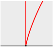
Figure 1. $a$ is to the right of $b$ in a neighborhood of $p$.

Suppose that $\varphi:\Sigma\to\Sigma$ is a homeomorphism of $\Sigma$ which restricts to the identity on a boundary component $B$ of $\Sigma$. Then we say that $\varphi$ is right-veering at $B$ if

$$\varphi(a)\geq_{p}a$$

for every properly-embedded arc $a\subset\Sigma$ and every $p\in\partial a\cap B$. If $\varphi$ restricts to the identity on all of $\partial\Sigma$, then we say that $\varphi$ is right-veering if

$$\varphi(a)\geq a$$

for every properly-embedded arc in $a\subset\Sigma$; equivalently, if $\varphi$ is right-veering at each boundary component of $\Sigma$. A map is left-veering if its inverse is right-veering.

As mentioned in the introduction, the notion of right-veering is important in low-dimensional topology due to the following theorem of Honda–Kazez–Matić [HKM07]:

Theorem 2.1.

A contact 3-manifold $(Y,\xi)$ is tight if and only if every fibered link $L\subset Y$ supporting $(Y,\xi)$ has right-veering monodromy.

A version of this result was stated in Theorem 1.1 in terms of fibered knots rather than links; we explain below how Theorem 1.1 follows from Theorem 2.1.

Proof of Theorem 1.1.

Suppose that $(Y,\xi)$ is tight. By Theorem 2.1, every fibered link—in particular, every fibered knot—supporting $(Y,\xi)$ has right-veering monodromy, proving one direction of Theorem 1.1.

For the other direction, let us suppose that every fibered knot supporting $(Y,\xi)$ has right-veering monodromy. We must show that $(Y,\xi)$ is tight. By Theorem 2.1, it suffices to prove that every fibered link supporting $(Y,\xi)$ has right-veering monodromy. We will prove this by induction on the number of link components (the base case holds by assumption).

Suppose that every fibered link supporting $(Y,\xi)$ with $n$ components has right-veering monodromy. Let $L\subset Y$ be a fibered link supporting $(Y,\xi)$ with $n+1$ components, with fiber $\Sigma$ and monodromy $\varphi$. Suppose, for a contradiction, that $a\subset\Sigma$ is a properly-embedded arc which is not sent to the right by $\varphi$. Let $c\subset\Sigma$ be an arc disjoint from $\varphi(a)$ whose endpoints lie on two different boundary components of $\Sigma$. Let $\Sigma^{\prime}$ be the surface obtained from $\Sigma$ by attaching a 1-handle along the endpoints of $c$, and let $\gamma\subset\Sigma^{\prime}$ be the curve obtained as the union of $c$ with a core of this handle. Letting $D_{\gamma}$ denote a right-handed Dehn twist about $\gamma$, we observe that the homeomorphism

$$\varphi^{\prime}=D_{\gamma}\circ\varphi$$

does not send $a\subset\Sigma^{\prime}$ to the right either, and is therefore not right-veering. As the open book $(\Sigma^{\prime},\varphi^{\prime})$ is a positive stabilization of $(\Sigma,\varphi)$, the associated fibered link $L^{\prime}\subset Y$ also supports $(Y,\xi)$. But $L^{\prime}$ has $n$ components, so its monodromy $\varphi^{\prime}$ is right-veering, a contradiction. ∎

2.2. Fractional Dehn twist coefficients

One can quantify how right-veering a homeomorphism is using the notion of fractional Dehn twist coefficient, as introduced by Honda–Kazez–Matić in [HKM07]. We explain this notion below in terms of certain standard representatives of surface homeomorphisms.

Let $\varphi:\Sigma\to\Sigma$ be a homeomorphism of a surface $\Sigma$. We say that $\varphi$ is periodic if $\varphi^{n}=\operatorname{id}$ for some positive integer $n$; when $\chi(\Sigma)<0$, we will assume that $\varphi$ is an isometry with respect to a hyperbolic metric on $\Sigma$ for which $\partial\Sigma$ is a geodesic. We say instead that $\varphi$ is pseudo-Anosov if there is a transverse pair of singular measured foliations

$$(\mathcal{F}_{s},\mu_{s})\textrm{ and }(\mathcal{F}_{u},\mu_{u})$$

of $\Sigma$, called the stable and unstable foliations of $\varphi$, such that

$$\varphi(\mathcal{F}_{s},\mu_{s})=(\mathcal{F}_{s},\lambda^{-1}\mu_{s})\textrm{ and }\varphi(\mathcal{F}_{u},\mu_{u})=(\mathcal{F}_{u},\lambda\mu_{u})$$

for some real number $\lambda>1$. These foliations meet $\partial\Sigma$ in a finite number of singular leaves called prongs.

Suppose that $\varphi$ is pseudo-Anosov and fixes a component $B$ of $\partial\Sigma$ setwise. Let $p_{1},\dots,p_{k}$ denote the intersection points of $B$ with the prongs of the stable foliation of $\varphi$, ordered according to the orientation of $B$. Then there is an integer $n$ such that

$$\varphi(p_{m})=p_{m+n}$$

for all $m$, where the subscripts are taken mod $k$. The restriction of $\varphi$ to $B$ is thus isotopic rel $\{p_{1},\dots,p_{k}\}$ to a rotation by $2\pi n/k$. One can perturb $\varphi$ via isotopy rel $\{p_{1},\dots,p_{k}\}$ in a standard way, described in [CC09, §4.2], to a smooth map which restricts to $B$ as a rotation by $2\pi n/k$ on the nose. We will henceforth assume when talking about pseudo-Anosov maps that they are of this perturbed form. In particular, we will assume that both periodic and pseudo-Anosov homeomorphisms of a surface restrict to periodic maps on the boundary. We use these notions to define standard representatives of surface homeomorphisms below, closely following [CC09, Definition 4.6].

Suppose that $\varphi:\Sigma\to\Sigma$ is a homeomorphism of a surface $\Sigma$. By Thurston’s classification of surface homeomorphisms [Thu88], $\varphi$ is isotopic to a homeomorphism $\phi$ of the following form. There is a finite union $N$ of disjoint closed annuli and curves in $\Sigma$ which is invariant under $\phi$ and $\phi^{-1}$ such that:

• If $A$ is an annulus component of $N$, and $\ell$ is the smallest positive integer such that $\phi^{\ell}(A)=A$, then $\phi^{\ell}|_{A}$ is either a twist map or a flip-twist map. That is, with respect to an identification

  $$A\cong[0,1]\times\mathbb{R}/\mathbb{Z},$$

  the map $\phi^{\ell}|_{A}$ takes one of the following two forms:

  (twist) $$(q,p)\mapsto(q,p+f(q)),$$

  (flip-twist) $$(q,p)\mapsto(1-q,-p-f(q)),$$

  where $f:[0,1]\to\mathbb{R}$ is a strictly monotonic smooth map such that $\phi^{\ell}|_{A}$ restricts to a periodic map on every boundary component of $A$ which is disjoint from $\partial\Sigma$.
  

• Let $A$ and $\ell$ be as above. If $\ell=1$ and $\phi|_{A}$ is a twist map, then $\textrm{Im}(f)\subset[0,1]$. Such an annulus $A$ is called a twist region, and is positive or negative if $f$ is increasing or decreasing, respectively. We require that parallel twist regions have the same sign. If $\ell=1$ and $\phi|_{A}$ is a flip-twist map, then $A$ is called a flip-twist region.
  

• Let $S$ be the closure of a component of $\Sigma\setminus N$, and $\ell$ the smallest positive integer such that $\phi^{\ell}(S)=S$. Then $\phi^{\ell}|_{S}$ is either periodic or pseudo-Anosov. We call $S$ a fixed component if $\ell=1$ and $\phi|_{S}=\operatorname{id}$. We require that $S$ is fixed if it is an annulus. In particular, parallel twist regions are separated by fixed annuli. A multitwist region is a maximal annular subsurface of $\Sigma$ given as a union of twist regions and the fixed annuli between them.
  

• $N$ is called the invariant set for $\phi$. We will assume that it is minimal with respect to inclusion. In particular, there is no curve component of $N$ which abuts a fixed region on both sides. There is a canonical such $N$ up to isotopy.

The map $\phi$ is called a standard representative of $\varphi$.

Remark 2.2.

A multitwist region $R$ consists of some number $k\geq 0$ of twist regions on which $\phi$ is a full Dehn twist, and at most two twist regions, each at an end of $R$, on which $\phi$ is a partial Dehn twist. In particular, if $R$ abuts a boundary component on which $\phi$ is the identity, then $R$ has at most one partial twist region, at an end interior to the surface, as described below and illustrated in Figure 2. We will encounter multitwist regions with up to two partial twist regions in the proof of Proposition 4.1, as illustrated in Figure 4.

Suppose that $\varphi:\Sigma\to\Sigma$ is a homeomorphism of a surface $\Sigma$ which restricts to the identity on a boundary component $B$, and let $\phi$ be a standard representative of $\varphi$. The fractional Dehn twist coefficient of $\varphi$ at $B$, denoted by

$$c_{B}(\varphi)\in\mathbb{Q},$$

is defined as follows. If $B$ does not abut a multitwist region for $\phi$, then

$$c_{B}(\varphi)=0.$$

If $B$ does abut a multitwist region $R$, then for some integer $k\geq 0$ and some $\epsilon\in\{\pm 1\}$, $R$ is a union of $k+1$ twist regions

$$A_{1},\dots,A_{k+1}\cong[0,1]\times\mathbb{R}/\mathbb{Z},$$

together with the $k$ fixed annuli between them, where:

• $B$ is identified with $\{0\}\times\mathbb{R}/\mathbb{Z}\subset A_{1},$

• $\phi|_{A_{i}}$ is isotopic to the map

  $$(q,p)\to(q,p+\epsilon q),$$

  for each $i=1,\dots,k$, and

• $\phi|_{A_{k+1}}$ is isotopic to the map

  $$(q,p)\to(q,p+rq)$$

  for some rational number $r$ with $|r|\in(0,1).$

That is, $\varphi$ is a full $\epsilon$-twist on each of $A_{1},\dots,A_{k}$, and a partial twist on $A_{k+1}$, as indicated in Figure 2. In this case, we define

$$c_{B}(\varphi)=\epsilon k+r.$$

These twist coefficients satisfy

$$c_{B}(\varphi^{n})=nc_{B}(\varphi)\textrm{ and }c_{B}(\varphi^{-1})=-c_{B}(\varphi).$$

If $\Sigma$ has connected boundary, we denote the twist coefficient simply by $c(\varphi)$.

2pt $R$ at 139 313 $B$ at -1 148 $A_{1}$ at 70 0 $A_{2}$ at 135 0 $A_{3}$ at 200 0

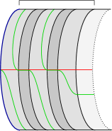
Figure 2. A portion of $\Sigma$ near the multitwist region $R$ in the case $k=2$ and $\epsilon=+1$. That is, $R$ is made up of three positive twist regions, $A_{1},A_{2},A_{3}$, shaded in medium gray, together with the two fixed annuli between them, shaded in dark gray. The green arc is the image of the red under $\phi$. In this example, we see that $c_{B}(\varphi)\in(2,3)$.

Fractional Dehn twist coefficients are intimately related with the notion of right-veering, as illustrated by Lemma 2.3 below. This lemma follows mostly from the work in [HKM07], but appears as stated below (or in a transparently equivalent way) in [KR13, Corollary 2.6].

Lemma 2.3.

Let $\varphi:\Sigma\to\Sigma$ be a homeomorphism which restricts to the identity on $\partial\Sigma$, and let $B$ be a boundary component of $\Sigma$. If $\varphi$ is right-veering at $B$ then $c_{B}(\varphi)\geq 0$. Moreover, if $c_{B}(\varphi)>0$ then $\varphi$ is right-veering at $B$. ∎

This lemma has the immediate corollary that if $\varphi$ is neither right-veering nor left-veering, then $c_{B}(\varphi)=0$, as noted in Remark 1.6.

Lemma 2.4.

Let $\varphi:\Sigma\to\Sigma$ be a pseudo-Anosov homeomorphism which restricts to the identity on a boundary component $B$ such that $c_{B}(\varphi)=0.$ Then there is a properly-embedded arc $a\subset\Sigma$ with $\partial a\subset B$ such that $\varphi(a)\not\geq a$. In particular, $\varphi$ is not right-veering at $B$.

Proof.

Note that $\varphi^{n}$ restricts to the identity on $\partial\Sigma$ for some positive integer $n$, and

$$c_{B}(\varphi^{n})=nc_{B}(\varphi)=0.$$

Then [HKM07, Proposition 3.1] says that $\varphi^{n}$ is not right-veering at $B$. Moreover, the proof of that proposition shows that there is a properly-embedded arc $a\subset\Sigma$ with $\partial a\subset B$ such that $\varphi^{n}(a)\not\geq a$, from which it follows that $\varphi(a)\not\geq a$ as well. ∎

Lemma 2.5.

If $\varphi:\Sigma\to\Sigma$ is a periodic homeomorphism which restricts to the identity on a boundary component $B$ such that $c_{B}(\varphi)=0,$ then $\varphi=\operatorname{id}$.

Proof.

This follows, for instance, from [JG93, Lemma 1.1], which implies in our case that the entire surface $\Sigma$ is a connected component of the fixed point set of $\varphi$. ∎

The following lemma is key in our proof of Proposition 4.1, which explains how symplectic Floer homology detects right-veering monodromy.

Lemma 2.6.

Let $S$ be a surface with one boundary component. Let

$$h:S\to S$$

be a homeomorphism which restricts to the identity on the boundary, and let $\alpha$ be a standard representative of $h$ with invariant set $N$. Let $S_{0}$ denote the closure of the component of $S\setminus N$ which abuts either $\partial S$ or a multitwist region containing $\partial S$, and let

$$\alpha_{0}=\alpha|_{S_{0}}:S_{0}\to S_{0}.$$

Then $h$ is right-veering if and only if either:

1. $\partial S$ abuts a positive twist region for $\alpha$, or

2. $\partial S\subset\partial S_{0}$, $\alpha_{0}=\operatorname{id}$, and every boundary component of $S_{0}$ besides $\partial S$ abuts a positive twist region for $\alpha$.

Proof.

Suppose that $h$ is right-veering. Then $c(h)\geq 0$ by Lemma 2.3. If $c(h)>0$, then $\partial S$ abuts a positive twist region for $\alpha$, and we are done. Let us therefore suppose that $c(h)=0$. This implies that $\partial S\subset\partial S_{0}$, that $\alpha_{0}|_{\partial S}=h|_{\partial S}=\operatorname{id}$, and that

$$c_{\partial S}(\alpha_{0})=c(h)=0.$$

Observe that $h$ is not freely isotopic to a pseudo-Anosov map, by [HKM07, Proposition 3.1]. If $h$ is freely isotopic to a periodic map, then Lemma 2.5 implies that $\alpha_{0}=\operatorname{id}$, as desired. There are no boundary components of $S_{0}$ besides $\partial S$ in this case.

Suppose, therefore, that $h$ is freely isotopic to a reducible map. If $\alpha_{0}$ is pseudo-Anosov, then the fact that $c_{\partial S}(\alpha_{0})=0$ implies by Lemma 2.4 that there is a properly-embedded arc $a\subset S_{0}$ with $\partial a\subset\partial S$ such that

$$h(a)\sim\alpha_{0}(a)\not\geq a,$$

which contradicts the assumption that $h$ is right-veering. Thus, $\alpha_{0}$ is periodic, which implies that $\alpha_{0}=\operatorname{id}$ by Lemma 2.5. It remains to show that every component $B$ of $\partial S_{0}\setminus\partial S$ abuts a positive twist region for $\alpha$. It is easy to see that the restriction

$$\alpha^{\prime}=\alpha|_{S\setminus\textrm{int}(S_{0})}$$

is right-veering at $B$, given that $h$ is right-veering and $\alpha_{0}=\operatorname{id}$. Thus, $c_{B}(\alpha^{\prime})\geq 0$ by Lemma 2.3. If $c_{B}(\alpha^{\prime})>0$, then $B$ abuts a positive twist region. Suppose, for a contradiction, that $c_{B}(\alpha^{\prime})=0$. Then $B$ does not abut any twist region; instead, $B$ abuts a component

$$S^{\prime}\subset S\setminus\textrm{int}(S_{0})$$

on which $\alpha^{\prime}$ is either pseudo-Anosov or periodic. In the first case, Lemma 2.4 says that there is a properly-embedded arc $a\subset S^{\prime}$ with $\partial a\subset B$ such that $\alpha^{\prime}(a)\not\geq a$, but this contradicts the fact that $\alpha^{\prime}$ is right-veering. In the second case, Lemma 2.5 implies that $\alpha^{\prime}$ restricts to the identity on $S^{\prime}$. But since $\alpha_{0}=\operatorname{id}$, this contradicts the minimality of the invariant set for $\alpha$: there should not be a curve abutting two regions on which $\alpha$ is the identity.

For the other direction, suppose first that item (1) of the lemma holds. Then $c(h)>0$, which implies that $h$ is right-veering by Lemma 2.3. Suppose now that item (2) holds. Then the fractional Dehn twist coefficients of the restriction

$$\alpha^{\prime}=\alpha|_{S\setminus\textrm{int}(S_{0})}$$

are all positive. The map $\alpha^{\prime}$ is thus right-veering by Lemma 2.3. Since $S$ is obtained from $S\setminus\textrm{int}(S_{0})$ by attaching 1-handles, and $\alpha$ is the extension of $\alpha^{\prime}$ to $S$ by the identity, [HKM07, Lemma 2.3] says that $\alpha$ and therefore $h\sim\alpha$ is right-veering as well. ∎

2.3. Symplectic Floer homology

Suppose $\varphi:\Sigma\to\Sigma$ is a homeomorphism of a closed surface $\Sigma$. Let $\omega$ be an area form on $\Sigma$, and let $\phi$ be an area-preserving diffeomorphism of $\Sigma$ isotopic to $\varphi$. Assuming certain nondegeneracy and monotonicity conditions, the symplectic Floer homology $\mathit{HF}^{symp}(\varphi)$ is the homology of a chain complex $\mathit{CF}^{symp}(\phi)$ which is freely-generated as an $\mathbb{F}$-vector space by the fixed points of $\phi$, and whose differential counts certain holomorphic cylinders. As indicated by the notation and proved by Seidel in [Sei02], the $\mathbb{F}$-vector space $\mathit{HF}^{symp}(\varphi)$ depends up to isomorphism only on the mapping class of $\varphi$.

The goal of this section is to review Cotton-Clay’s calculation of symplectic Floer homology in terms of standard representatives (Theorem 2.8). We first establish some notation.

Let $\varphi:\Sigma\to\Sigma$ be a homeomorphism of a closed surface $\Sigma$, and let $\phi$ be a standard representative of $\varphi$. Let $\Sigma_{0}$ denote the collection of fixed components for $\phi$. Let $\Sigma_{1}$ be the collection of (non-fixed) periodic components, and let $\Sigma_{2}$ be the collection of pseudo-Anosov components. We further divide $\Sigma_{0}$ into three subcollections as follows.

Let $\Sigma_{a}$ be the collection of fixed components for $\phi$ which do not abut any pseudo-Anosov components. Let $\Sigma_{b,p}$ be the collection of fixed components which abut exactly one pseudo-Anosov component, at a boundary with $p$ prongs. Let $\Sigma_{b,p}^{\circ}$ denote the subsurface obtained from $\Sigma_{b,p}$ by removing an open disk from each component of $\Sigma_{b,p}$. Let $\Sigma_{c,q}$ be the collection of fixed components $S$ which abut at least two pseudo-Anosov components, such that the total number of prongs meeting the boundary of $S$ is $q$.

Remark 2.7.

A fixed component cannot abut a periodic component $S$; otherwise, $\phi$ would restrict to the identity on a boundary component $B$ of $S$ and would satisfy

$$c_{B}(\phi|_{S})=0.$$

This would imply by Lemma 2.5 that $\phi$ is the identity on $S$, violating the minimality of the invariant set for $\phi$.

We partition $\partial\Sigma_{0}$ into collections $\partial_{\pm}\Sigma_{0}$ of positive and negative components as follows. Suppose that $S\subset\Sigma_{0}$ is a fixed component. If a component of $\partial S$ abuts a positive or negative twist region, then it is assigned to $\partial_{\pm}\Sigma_{0}$, respectively. If $S\subset\Sigma_{b,p}$, then the component of $\partial S$ which abuts a pseudo-Anosov component is assigned to $\partial_{-}\Sigma_{0}$. If $S\subset\Sigma_{c,q}$, then we assign at least one component of $\partial S$ which meets a pseudo-Anosov component to $\partial_{-}\Sigma_{0}$ and at least one other to $\partial_{+}\Sigma_{0}$ (and beyond that, it does not matter).

In [CC09, §4.5], Cotton-Clay further perturbs $\phi$ to an area-preserving diffeomorphism $\hat{\phi}$ of $\Sigma$ (with respect to some area form) with isolated fixed points, which agrees with $\phi$ on the invariant set. Let $\Lambda(\hat{\phi}|_{\Sigma_{1}})$ be the Lefschetz number of $\hat{\phi}|_{\Sigma_{1}}$. Let

$$\mathit{CF}^{symp}(\hat{\phi}|_{\Sigma_{2}})$$

denote the symplectic Floer chain complex for $\hat{\phi}$ restricted to $\Sigma_{2}$, understood as the $\mathbb{F}$-vector space freely-generated by the fixed points of $\hat{\phi}|_{\Sigma_{2}}$ which are not contained in $\partial\Sigma_{2}$.

Let $n_{f}$ denote the number of flip-twist regions for $\phi$.

With this setup, we are finally ready to state Cotton-Clay’s formula for symplectic Floer homology [CC09, Theorem 4.16], as clarified slightly in [Ni22, Theorem 1.3]:

Theorem 2.8.

Suppose that $\varphi:\Sigma\to\Sigma$ is a homeomorphism of a closed surface $\Sigma$ with $g(\Sigma)\geq 2$, and let $\phi$ be a standard representative of $\varphi$. Then we have that

$$\mathit{HF}^{symp}(\varphi)\cong\,\, H_{*}(\Sigma_{a},\partial_{-}\Sigma_{a};\mathbb{F})$$

$$\oplus\bigoplus_{p}\Big{[}H_{*}(\Sigma_{b,p}^{\circ},\partial_{-}\Sigma_{b,p};\mathbb{F})\oplus\mathbb{F}^{(p-1)|\pi_{0}(\Sigma_{b,p})|}\Big{]}$$

$$\oplus\bigoplus_{q}\Big{[}H_{*}(\Sigma_{c,p},\partial_{-}\Sigma_{c,q};\mathbb{F})\oplus\mathbb{F}^{q|\pi_{0}(\Sigma_{c,q})|}\Big{]}$$

$$\oplus\mathbb{F}^{\Lambda(\hat{\phi}|_{\Sigma_{1}})}\oplus\mathbb{F}^{2n_{f}}\oplus\mathit{CF}^{symp}(\hat{\phi}|_{\Sigma_{2}}),$$

with respect to the notation introduced above.

Remark 2.9.

Since the relative homology groups of fixed regions contribute importantly in the formula above, we remind the reader that if $S$ is a surface with boundary, and $\partial_{-}S$ is subcollection of the components of $\partial S$, then

$$\dim H_{*}(S,\partial_{-}S;\mathbb{F})=\begin{cases}\dim H_{*}(S;\mathbb{F}),&\textrm{ if }\partial_{-}S=\emptyset\textrm{ or }\partial_{-}S=\partial S,\\ \dim H_{*}(S;\mathbb{F})-2,&\textrm{ otherwise}.\end{cases}$$

We will use this extensively in the proof of Proposition 4.1.

Remark 2.10.

The contributions from $\Sigma_{0}$, $\Sigma_{1}$, $\Sigma_{2}$ to the formula in Theorem 2.8 do not change if we replace $\phi$ with $\phi^{-1}$. In particular, $\mathit{HF}^{symp}(\varphi)\cong\mathit{HF}^{symp}(\varphi^{-1}).$

We end by describing the relationship between symplectic Floer homology and Heegaard Floer homology. For this, suppose that $\varphi:\Sigma\to\Sigma$ is a homeomorphism of a closed surface $\Sigma$ with $g(\Sigma)\geq 2$. Let $M_{\varphi}$ denote the mapping torus of $\varphi$. Let us define

$$\mathit{HF}^{+}(M_{\varphi},\mathrm{top}{-}1)=\bigoplus_{\begin{subarray}{c}\mathfrak{s}\in\operatorname{Spin}^{c}(M_{\varphi})\\ \langle c_{1}(\mathfrak{s}),[\Sigma]\rangle=2g(\Sigma)-4\end{subarray}}\mathit{HF}^{+}(M_{\varphi},\mathfrak{s}).$$

The result below is a combination of work by Lee–Taubes [LT12, Theorem 1.1] and Kutluhan–Lee–Taubes [KLT20, Main Theorem]:

Theorem 2.11.

Suppose that $\varphi:\Sigma\to\Sigma$ is a homeomorphism of a closed surface $\Sigma$ with $g(\Sigma)\geq 3$. Then

$$\mathit{HF}^{+}(M_{\varphi},\mathrm{top}{-}1)\cong\mathit{HF}^{symp}(\varphi).$$

We will apply this theorem in §4 to mapping tori arising as $0$-surgery on the fibered knots $J_{\pm}\subset Z$ introduced in §3 in order to prove our main Theorem 1.3.

2.4. Knot Floer homology and $b$

We assume below that the reader has some familiarity with Heegaard Floer homology. Our goals in this section are primarily to establish notation and review the invariant $b$. See [OS04, BVV18] for more background.

Suppose that $(\Sigma,\alpha,\beta,z,w)$ is a doubly-pointed Heegaard diagram for a nullhomologous knot $K\subset Y$. Recall that the Heegaard Floer chain complex

$$\widehat{\mathit{CF}}(Y)=\widehat{\mathit{CF}}(\Sigma,\alpha,\beta,w)$$

is the $\mathbb{F}$-vector space freely-generated by intersection points between the associated tori

$$\mathbb{T}_{\alpha},\mathbb{T}_{\beta}\subset\operatorname{Sym}^{k}(\Sigma),$$

where $k=g(\Sigma)$. The differential

$$\partial:\widehat{\mathit{CF}}(Y)\to\widehat{\mathit{CF}}(Y)$$

is the linear map defined on generators $\mathbf{x}\in\mathbb{T}_{\alpha}\cap\mathbb{T}_{\beta}$ by

$$\partial(\mathbf{x})=\sum_{\mathbf{y}\in\mathbb{T}_{\alpha}\cap\mathbb{T}_{\beta}}\sum_{\begin{subarray}{c}\phi\in\pi_{2}(\mathbf{x},\mathbf{y})\\ \mu(\phi)=1\\ n_{w}(\phi)=0\end{subarray}}\#\widehat{\mathcal{M}}(\phi)\cdot\mathbf{y},$$

where $\pi_{2}(\mathbf{x},\mathbf{y})$ denotes the set of homotopy classes of Whitney disks from $\mathbf{x}$ to $\mathbf{y}$, $\mu(\phi)$ is the Maslov index of $\phi$, $n_{w}(\phi)$ is the intersection number

$$\phi\cdot\big{(}\{w\}\times\operatorname{Sym}^{k-1}(\Sigma)\big{)},$$

and $\widehat{\mathcal{M}}(\phi)$ is the space of pseudo-holomorphic representatives of $\phi$ modulo conformal automorphisms of the domain. The chain homotopy type of this complex, and thus the Heegaard Floer homology group

$$\widehat{\mathit{HF}}(Y)=H_{*}(\widehat{\mathit{CF}}(Y),\partial),$$

is an invariant of $Y$.

Given a Seifert surface $S$ for the knot $K$, each generator $\mathbf{x}$ of the Heegaard Floer complex is assigned an Alexander grading

$$A(\mathbf{x})\in\mathbb{Z}$$

such that for generators $\mathbf{x}$ and $\mathbf{y}$ connected by a Whitney disk $\phi\in\pi_{2}(\mathbf{x},\mathbf{y})$, we have

(2.1) $$A(\mathbf{x})-A(\mathbf{y})=n_{z}(\phi)-n_{w}(\phi).$$

Let $\mathscr{F}_{i}$ denote the subspace of $\widehat{\mathit{CF}}(Y)$ spanned by generators in Alexander grading at most $i$. The fact that $n_{z}(\phi)\geq 0$ when $\phi$ has a pseudo-holomorphic representative, combined with (2.1) and the fact that $\partial$ counts disks with $n_{w}(\phi)=0$, implies that these subspaces are in fact subcomplexes, and that they define a filtration

$$\dots\subset\mathscr{F}_{n-2}\subset\mathscr{F}_{n-1}\subset\mathscr{F}_{n}=\widehat{\mathit{CF}}(Y).$$

The filtered chain homotopy type of this complex is an invariant of $(Y,K)$ and the relative homology class $[S]\in H_{2}(Y,K)$. We denote by

$$\widehat{\mathit{CFK}}(Y,K,[S],i)=\mathscr{F}_{i}/\mathscr{F}_{i-1}$$

the direct summand of the associated graded complex in Alexander grading $i$, and by

$$\widehat{\mathit{HFK}}(Y,K,[S],i)=H_{*}(\widehat{\mathit{CFK}}(Y,K,[S],i))$$

the resulting knot Floer homology group in Alexander grading $i$. Recall that

(2.2) $$\widehat{\mathit{HFK}}(Y,K,[S],i)=0\textrm{ for }|i|>g(S).$$

Letting

$$\widehat{\mathit{HFK}}(Y,K,[S])=\bigoplus_{i}\widehat{\mathit{HFK}}(Y,K,[S],i),$$

it follows that the filtration above gives rise to a spectral sequence with

$$E_{1}\cong\widehat{\mathit{HFK}}(Y,K,[S])\textrm{ and }E_{\infty}\cong\widehat{\mathit{HF}}(Y)$$

whose $d_{1}$ differential is a sum over integers $i$ of maps of the form

$$d_{1}:\widehat{\mathit{HFK}}(Y,K,[S],i)\to\widehat{\mathit{HFK}}(Y,K,[S],i-1).$$

The chain complexes above (and thus the corresponding homology groups) split as direct sums of complexes over $\operatorname{Spin}^{c}$ structures on $Y$. Given $\mathfrak{s}\in\operatorname{Spin}^{c}(Y)$, we denote by

$$\widehat{\mathit{CF}}(Y,\mathfrak{s}),\,\widehat{\mathit{HF}}(Y,\mathfrak{s}),\,\widehat{\mathit{CFK}}(Y,K,[S],\mathfrak{s},i),\,\widehat{\mathit{HFK}}(Y,K,[S],\mathfrak{s},i)$$

the corresponding $\operatorname{Spin}^{c}$ summands.

Remark 2.12.

For a knot $K\subset S^{3}$, we have that

$$E_{\infty}\cong\widehat{\mathit{HF}}(S^{3})\cong\mathbb{F}.$$

The tau invariant $\tau(K)\in\mathbb{Z}$ is the Alexander grading of the generator of this page.

Remark 2.13.

We will omit the Seifert surface $S$ from the notation above where the class $[S]$ is implicit, as in the case of a fibered knot or a knot in a rational homology sphere.

Remark 2.14.

The knot Floer homology of a knot $K\subset S^{3}$ is bigraded,

$$\widehat{\mathit{HFK}}(S^{3},K)=\bigoplus_{m,i}\widehat{\mathit{HFK}}_{m}(S^{3},K,i),$$

where $m\in\mathbb{Z}$ denotes the Maslov grading. The knot Floer homology is thin if it is supported in bigradings $(m,i)$ with $m-i$ constant. The fact that the differential $\partial$ shifts Maslov grading by $-1$ implies that the spectral sequence

$$E_{1}\cong\widehat{\mathit{HFK}}(S^{3},K)\implies\widehat{\mathit{HF}}(S^{3})\cong E_{\infty}$$

collapses at the $E_{2}$ page when the knot Floer homology of $K$ is thin.

Suppose now that $K\subset Y$ is a fibered knot of genus $g$. Then

(2.3) $$\widehat{\mathit{HFK}}(\pm Y,K,\pm g)\cong\mathbb{F}.$$

Moreover, if $\mathfrak{s}$ is the $\operatorname{Spin}^{c}$ structure on $Y$ associated with the fibration of $K$ (by which we mean the $\operatorname{Spin}^{c}$ structure associated with the contact structure on $Y$ supported by $K$), then

(2.4) $$\widehat{\mathit{HFK}}(Y,K,\mathfrak{s},g) \cong\mathbb{F},$$

(2.5) $$\widehat{\mathit{HFK}}(Y,K,\mathfrak{s}^{\prime},g) =0,\textrm{ for }\mathfrak{s}^{\prime}\neq\mathfrak{s}.$$

Note that the combination of (2.2) and (2.3) implies that the filtration of $\widehat{\mathit{CF}}(-Y)$ associated with $K\subset-Y$ is filtered chain homotopy equivalent to a filtration of the form

$$\emptyset=\mathscr{F}_{-1-g}\,\subset\,\mathbb{F}\langle\mathbf{c}\rangle=\mathscr{F}_{-g}\,\subset\,\mathscr{F}_{1-g}\,\subset\,\cdots\,\subset\mathscr{F}_{g}=\widehat{\mathit{CF}}(-Y),$$

as mentioned in the introduction. As in that section, we define the invariant

$$b(K)=b(K\subset Y)\in\mathbb{N}\cup\{\infty\}$$

to be either

$$g+\min\{k\mid[\mathbf{c}]=0\textrm{ in }H_{*}(\mathscr{F}_{k})\},$$

if $[\mathbf{c}]=0\textrm{ in }\widehat{\mathit{HF}}(-Y),$ or $\infty$ otherwise. The spectral sequence interpretation of $b$ in Remark 1.4 then follows readily from its definition and the discussion above.

Theorem 1.2 is equivalent to the statement that $b(K)=1$ when the monodromy of $K$ is not right-veering. As mentioned in the introduction, this was proved by Baldwin–Vela-Vick via a Heegaard-diagrammatic approach, but it is not clear how to prove our main Theorem 1.3 by a similarly direct strategy. We elaborate on this point below.

The idea behind Baldwin–Vela-Vick’s proof of Theorem 1.2 is roughly the following: suppose that the monodromy $h:S\to S$ of $K$ is not right-veering. Then there is some basis arc $a\subset S$ which is not sent to the right by $h$. This arc and its image $h(a)$ can be used to define attaching curves in a doubly-pointed Heegaard diagram for $K\subset-Y$. The fact that $h$ does not send $a$ to the right is used to find a generator

$$\mathbf{d}\in\widehat{\mathit{CF}}(-Y),$$

in Alexander grading $1-g,$ such that the sole contribution to $\partial\mathbf{d}$ is a pseudo-holomorphic disk with domain given by a bigon from $\mathbf{d}$ to $\mathbf{c}$. This proves that $b(K)=1$.

One might hope to prove the converse (our Theorem 1.3) by similar diagrammatic means, working in reverse. More precisely, given a doubly-pointed Heegaard diagram for $K$ adapted to the open book $(S,h)$ and a basis of arcs on $S$, one might hope that $b(K)=1$ implies that there is a bigon from a generator $\mathbf{d}$ as above to $\mathbf{c}$, certifying that at least one of the basis arcs is not sent to the right. However, this strategy fails for the reason that one can find a surface $S$, a monodromy $h:S\to S$, and a basis of arcs on $S$ such that $h$ is not right-veering but nevertheless moves every arc in the basis to the right, as illustrated in Figure 3 below.

2pt $S$ at 53 48

$x$ at 142 7 $y$ at 7 142 $a$ at 7 89 $b$ at 7 166

$h(a)$ at 358 102 $h(b)$ at 358 60

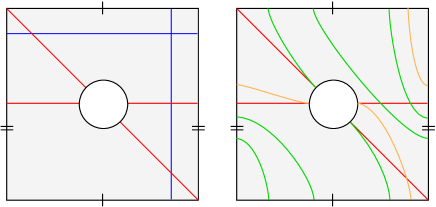
Figure 3. The composition $h=D_{x}\circ D_{y}^{-1}$ of a right-handed Dehn twist about $x$ with a left-handed Dehn twist about $y$ is a non-right-veering homeomorphism of the once-punctured torus $S$. The arcs $a$ and $b$ form a basis for $S$, and are both moved to the right by $h$.

2.5. The infinity knot Floer complex

We end this section with a review of the $\mathit{CFK}^{\infty}$ version of the knot Floer complex, which we will use extensively in §3.

Given a doubly-pointed Heegaard diagram for a nullhomologous knot $K\subset Y$ with Seifert surface $S$ as in the previous section, the chain complex

$$\mathscr{C}=\mathit{CFK}^{\infty}(Y,K,[S])$$

is generated as a vector space over $\mathbb{F}$ by triples $[\mathbf{x},i,j]$, with $\mathbf{x}\in\mathbb{T}_{\alpha}\cap\mathbb{T}_{\beta}$ and $(i,j)\in\mathbb{Z}\oplus\mathbb{Z}$, satisfying

$$A(\mathbf{x})=j-i.$$

This complex has the structure of an $\mathbb{F}[U]$-module, where multiplication by $U$ acts as

$$U\cdot[\mathbf{x},i,j]=[\mathbf{x},i-1,j-1].$$

The differential

$$\delta:\mathscr{C}\to\mathscr{C}$$

is the $\mathbb{F}[U]$-module map defined on generators by

$$\delta([\mathbf{x},i,j])=\sum_{\mathbf{y}\in\mathbb{T}_{\alpha}\cap\mathbb{T}_{\beta}}\sum_{\begin{subarray}{c}\phi\in\pi_{2}(\mathbf{x},\mathbf{y})\\ \mu(\phi)=1\end{subarray}}\#\widehat{\mathcal{M}}(\phi)\cdot[\mathbf{y},i-n_{w}(\phi),j-n_{z}(\phi)].$$

The complex $(\mathscr{C},\delta)$ is $(\mathbb{Z}\oplus\mathbb{Z})$-filtered with respect to the grading which assigns to a generator $[\mathbf{x},i,j]$ the pair $(i,j)$, once again by the nonnegativity of $n_{z}(\phi)$ and $n_{w}(\phi)$ for disks $\phi$ which admit pseudo-holomorphic representatives. In particular, $\delta$ is a sum of maps

$$\delta=\sum\delta_{mn}$$

over pairs of nonnegative integers, where $\delta_{mn}$ is the component of $\delta$ which lowers the grading by $(m,n).$ As before, the filtered chain homotopy type is an invariant of $(Y,K,[S])$, and this complex splits as a direct sum of complexes over $\operatorname{Spin}^{c}$ structures on $Y$. We will denote by $\mathscr{C}_{\mathfrak{s}}$ the summand corresponding to $\mathfrak{s}\in\operatorname{Spin}^{c}(Y)$.

Given $(i,j)\in\mathbb{Z}\oplus\mathbb{Z}$, let $\mathscr{C}_{\mathfrak{s}}(i,j)$ be the subspace of $\mathscr{C}_{\mathfrak{s}}$ spanned by generators of the form $[\mathbf{x},i,j]$. Then the component $\delta_{mn}$ of $\delta$ restricts to a sum of maps of the form

$$\delta_{mn}:\mathscr{C}_{\mathfrak{s}}(i,j)\to\mathscr{C}_{\mathfrak{s}}(i-m,j-n)$$

over pairs of integers $(i,j)$. More generally, given a subset $X\subset\mathbb{Z}\oplus\mathbb{Z}$, we define

$$\mathscr{C}_{\mathfrak{s}}X=\bigoplus_{(i,j)\in X}\mathscr{C}_{\mathfrak{s}}(i,j).$$

The differential $\delta$ induces an endomorphism of $\mathscr{C}_{\mathfrak{s}}X$ which may or may not be a differential. For example, $\mathscr{C}_{\mathfrak{s}}(i,j)$ is naturally a chain complex with respect to the induced map $\delta_{00}$, and there is a canonical isomorphism of this complex with the knot Floer complex above,

$$\mathscr{C}_{\mathfrak{s}}(i,j)\cong\widehat{\mathit{CFK}}(Y,K,[S],\mathfrak{s},j-i).$$

Moreover, for each $k\in\mathbb{Z}$, the induced endomorphism

$$\delta_{00}+\delta_{01}+\delta_{02}+\dots$$

on $\mathscr{C}\{i=k\}$ is a differential which is filtered by the $j$-coordinate, and this filtered complex is isomorphic to $\widehat{\mathit{CF}}(Y)$ with its filtration induced by $K$ and $[S]$ as above. The same is true of the complex $\mathscr{C}\{j=k\}$ as filtered by the $i$-coordinate.

In practice, we will use the reduced model for $\mathit{CFK}^{\infty}(Y,K,[S])$. This is the $(\mathbb{Z}\oplus\mathbb{Z})$-filtered chain complex $(C,d)$ over $\mathbb{F}[U]$, where

$$C=H_{*}(\mathscr{C},\delta_{00})$$

is obtained by taking homology with respect to $\delta_{00}$, and $d$ is the induced differential on $C$. Extending the notational conventions above in the obvious way, we have that

$$C_{\mathfrak{s}}(i,j)\cong\widehat{\mathit{HFK}}(Y,K,[S],\mathfrak{s},j-i)$$

for each $\mathfrak{s}\in\operatorname{Spin}^{c}(Y)$ and $(i,j)\in\mathbb{Z}\oplus\mathbb{Z}$, and

$$d=\sum d_{mn}$$

is a sum of maps over pairs $(m,n)$ of nonnegative integers which are not both equal to zero, where each component $d_{mn}$ restricts to a map

$$d_{mn}:C_{\mathfrak{s}}(i,j)\to C_{\mathfrak{s}}(i-m,j-n)$$

for every $(i,j)$. In addition, multiplication by $U$ is a map

$$U:C_{\mathfrak{s}}(i,j)\to C_{\mathfrak{s}}(i-1,j-1).$$

This reduced complex $(C,d)$ is $(\mathbb{Z}\oplus\mathbb{Z})$-filtered chain homotopy equivalent to $(\mathscr{C},\delta)$. In particular, for each $k\in\mathbb{Z}$, the complex $C\{i=k\}$ with filtration induced by the $j$-coordinate, which as a vector space is given by

$$C\{i=k\}\,\cong\,\bigoplus_{j\in\mathbb{Z}}\widehat{\mathit{HFK}}(Y,K,[S],j-k),$$

is filtered chain homotopy equivalent to $\widehat{\mathit{CF}}(Y)$ with the filtration induced by $K$ and $[S]$ as above. Moreover, the restriction of

$$d_{01}=(\partial_{01})_{*}$$

to $C\{i=k\}$ is a sum over integers $j$ of maps of the form

$$d_{01}:\widehat{\mathit{HFK}}(Y,K,[S],j-k)\to\widehat{\mathit{HFK}}(Y,K,[S],j-k-1),$$

and agrees with the $d_{1}$ differential of the spectral sequence

$$\widehat{\mathit{HFK}}(Y,K,[S])\implies\widehat{\mathit{HF}}(Y).$$

The same holds for $C\{j=k\}$ and $d_{10}$.

3. The Heegaard Floer homology of $0$-surgery

The goal of this section is to prove Proposition 3.4 below. As outlined in the introduction, this result is a step in the proof of Theorem 1.3, which we will complete in the next section. We first establish some notation that will be used in this section and the next.

Let $\mathfrak{s}_{0}$ be a nontorsion $\operatorname{Spin}^{c}$ structure on $S^{1}\times S^{2}$. Work of Eliashberg [Eli89] implies that there is a contact structure $\xi$ with $\mathfrak{s}_{\xi}=\mathfrak{s}_{0}$. Let $L\subset S^{1}\times S^{2}$ be a fibered knot supporting $\xi$, with fiber $G$. Let $L_{+}\subset S^{1}\times S^{2}$ be the $(3,3n+1)$-cable of $L$ for $n\geq 1$. This cable is naturally fibered, with fiber given by

$$F=T\cup G_{1}\cup G_{2}\cup G_{3},$$

where $T$ is a genus-$3n$ surface with four boundary components, and the $G_{i}$ are copies of $G$. In particular,

$$g^{\prime}:=g(L_{+})=3g(L)+3n\geq 3.$$

Let $g_{+}:F\to F$ denote the monodromy of $L_{+}$. Then $g_{+}$ is reducible: it restricts to $T$ as a periodic map of period $9n+3$, and cyclically permutes the $G_{i}$. Let $L_{-}\subset S^{1}\times S^{2}$ denote the mirror of $L_{+}$, with monodromy $g_{-}:F\to F$ given by the inverse of $g_{+}$. The fibration of $L_{-}$ represents the conjugate $\operatorname{Spin}^{c}$ structure $\bar{\mathfrak{s}}_{0}$, which is also nontorsion.

Lemma 3.1.

The fractional Dehn twist coefficients of $g_{\pm}$ are given by

$$c(g_{\pm})=\pm 1/(9n+3).$$

Proof.

It is shown in [KR13, Proposition 4.2] that the $(p,q)$-cable of a fibered knot, for $p$ and $q$ relatively prime and $|p|>1$, has fractional Dehn twist coefficient $1/pq$. This is stated there for cables of fibered knots in $S^{3}$, but the proof is local and applies to cables of fibered knots in any 3-manifold; see also [Ni21a, Lemma 4.2]. ∎

The reason we ultimately consider cables is for the following lemma, which follows from work of Hedden [Hed05] and is a key input for Proposition 3.4.

Lemma 3.2.

For $n$ sufficiently large,

$$\widehat{\mathit{HFK}}(S^{1}\times S^{2},L_{\pm},g^{\prime}-2)=0,$$

and

$$\widehat{\mathit{HFK}}(S^{1}\times S^{2},L_{\pm},g^{\prime}-1)\cong\mathbb{F}$$

is supported in the $\operatorname{Spin}^{c}$ structures $\mathfrak{s}_{0}$ and $\bar{\mathfrak{s}}_{0}$, respectively.

Proof.

A slight adaptation of the proof of [Hed05, Lemma 3.6] shows that for $n$ sufficiently large, we have that

$$\widehat{\mathit{HFK}}(S^{1}\times S^{2},L_{+},\mathfrak{s},g^{\prime}-1)\cong\widehat{\mathit{HFK}}(S^{1}\times S^{2},L,\mathfrak{s},g)$$

for each $\mathfrak{s}\in\operatorname{Spin}^{c}(S^{1}\times S^{2})$, and that

$$\widehat{\mathit{HFK}}(S^{1}\times S^{2},L_{+},g^{\prime}-2)=0.$$

In particular, there is a doubly-pointed Heegaard diagram for the cable $L_{+}$ such that there is an isomorphism of chain complexes,

$$\widehat{\mathit{CFK}}(S^{1}\times S^{2},L_{+},\mathfrak{s},g^{\prime}-1)\cong\widehat{\mathit{CFK}}(S^{1}\times S^{2},L,\mathfrak{s},g)$$

for each $\mathfrak{s}$, and for which there are no generators in Alexander grading $g^{\prime}-2$. Since

$$\widehat{\mathit{HFK}}(S^{1}\times S^{2},L,g)\cong\mathbb{F}$$

is supported in the $\operatorname{Spin}^{c}$ structure $\mathfrak{s}_{0}$ by (2.4)-(2.5), the result for $L_{+}$ follows. The lemma then follows for $L_{-}$ from the symmetry of knot Floer homology under taking mirrors,

$$\widehat{\mathit{HFK}}(S^{1}\times S^{2},L_{+},\mathfrak{s},j)\cong\widehat{\mathit{HFK}}(S^{1}\times S^{2},L_{-},\bar{\mathfrak{s}},j),$$

which holds for each Alexander grading $j$ and each $\mathfrak{s}\in\operatorname{Spin}^{c}(S^{1}\times S^{2})$ [OS04, §3]. ∎

Remark 3.3.

We will hereafter assume that $n$ is large enough that the conclusion of Lemma 3.2 holds.

The rest of this section is devoted to proving Proposition 3.4 below. Our proof is inspired by the proofs of [Ni21a, Proposition 3.1] and [Ni22, Proposition 4.1].

Proposition 3.4.

Suppose $K\subset Y$ is a nontrivial fibered knot of genus $g$ satisfying

$$b(K\subset Y)=b(K\subset-Y)=1,$$

and let

$$J_{\pm}=K\#L_{\pm}\textrm{ and }Z=Y\#(S^{1}\times S^{2}).$$

Then

$$\dim\mathit{HF}^{+}(Z_{0}(J_{\pm}),\mathrm{top}{-}1)=\dim\widehat{\mathit{HFK}}(Y,K,g-1)-1.$$

Proof.

Let us denote the genus of $J_{+}$ by

$$\bar{g}:=g(J_{+})=g(L_{+})+g(K)=g^{\prime}+g.$$

Recall that there is a natural identification

$$\operatorname{Spin}^{c}(Z_{0}(J_{+}))\cong\operatorname{Spin}^{c}(Z)\times\mathbb{Z}.$$

More precisely, for every $\operatorname{Spin}^{c}$ structure $\mathfrak{t}$ on $Z$ and each integer $k$, there is a unique $\operatorname{Spin}^{c}$ structure $\mathfrak{t}_{k}$ on $Z_{0}(J_{+})$ determined by the conditions that

$$\mathfrak{t}_{k}|_{Z\setminus J_{+}}=\mathfrak{t}|_{Z\setminus J_{+}}\textrm{ and }\langle c_{1}(\mathfrak{t}_{k}),[S\cup F]\rangle=2k,$$

where we are viewing $S\cup F$ as the result of capping off the boundary connected sum $S\natural F$, which is the natural fiber surface for the knot $J_{+}=K\#L_{+}$. Moreover, every $\operatorname{Spin}^{c}$ structure on $Z_{0}(J_{+})$ arises in this way. Recall that

$$\mathit{HF}^{+}(Z_{0}(J_{+}),\mathrm{top}{-}1)$$

is the direct sum of the Heegaard Floer groups of $Z_{0}(J_{+})$ over $\operatorname{Spin}^{c}$ structures of the form $\mathfrak{t}_{\bar{g}-2}$. We will first show that this group is in fact supported in $\operatorname{Spin}^{c}$ structures $\mathfrak{t}_{\bar{g}-2}$, where

$$\mathfrak{t}\in\operatorname{Spin}^{c}(Z=Y\#(S^{1}\times S^{2}))$$

is of the form $\mathfrak{t}=\mathfrak{s}\#\mathfrak{s}_{0}$. We will then prove the dimension formula in the proposition.

Let $(C,d)$ be the reduced model for the $(\mathbb{Z}\oplus\mathbb{Z})$-filtered knot Floer complex

$$\mathit{CFK}^{\infty}(Z,J_{+}),$$

as described in §2.5. In particular, for each $\mathfrak{t}\in\operatorname{Spin}^{c}(Z)$, we have that

(3.1) $$C_{\mathfrak{t}}(i,j)\cong\widehat{\mathit{HFK}}(Z,J_{+},\mathfrak{t},j-i),$$

and $d=\sum d_{mn}$, where each component $d_{mn}$ is a sum of maps of the form

$$C_{\mathfrak{t}}(i,j)\to C_{\mathfrak{t}}(i-m,j-n).$$

This is a complex over $\mathbb{F}[U]$, where multiplication by $U$ is a map

$$U:C_{\mathfrak{t}}(i,j)\to C_{\mathfrak{t}}(i-1,j-1).$$

For each integer $k$, we consider the induced chain complexes

$$A^{+}_{k,\mathfrak{t}} =C_{\mathfrak{t}}\{\max(i,j-k)\geq 0\},$$

$$B^{+}_{\mathfrak{t}} =C_{\mathfrak{t}}\{i\geq 0\},$$

as in [OS08], where the latter is chain homotopy equivalent to $\mathit{CF}^{+}(Z,\mathfrak{t})$. There are two natural chain maps

$$v^{+}_{k},h^{+}_{k}:A^{+}_{k,\mathfrak{t}}\to B^{+}_{\mathfrak{t}}$$

where $v^{+}_{k}$ is vertical projection onto $C_{\mathfrak{t}}\{i\geq 0\}$; and $h^{+}_{k}$ is horizontal projection onto $C_{\mathfrak{t}}\{j\geq k\}$, followed by the identification of the latter with $C_{\mathfrak{t}}\{j\geq 0\}$ induced by multiplication by $U^{k}$, followed by a chain homotopy equivalence from $C_{\mathfrak{t}}\{j\geq 0\}$ to $C_{\mathfrak{t}}\{i\geq 0\}$.

One can compute the Floer homology of surgeries in terms of this data. For instance, the Heegaard Floer complex of $Z_{0}(J_{+})$ in the $\operatorname{Spin}^{c}$ structure $\mathfrak{t}_{k}$ is known to be chain homotopy equivalent to the mapping cone of $v^{+}_{k}+h^{+}_{k}$,

(3.2) $$\mathit{CF}^{+}(Z_{0}(J_{+}),\mathfrak{t}_{k})\simeq\operatorname{Cone}(v^{+}_{k}+h^{+}_{k}).$$

For a torsion $\operatorname{Spin}^{c}$ structure $\mathfrak{t}$, this follows exactly as in [OS08, §4.8]. For nontorsion $\mathfrak{t}$, this follows from [Ni20b, Theorem 3.1]. We use this extensively below.

Let us suppose first that $\mathfrak{t}=\mathfrak{s}\#\mathfrak{s}^{\prime}$ with $\mathfrak{s}^{\prime}\neq\mathfrak{s}_{0}$. As mentioned above, our aim in this case is to prove that

(3.3) $$\mathit{HF}^{+}(Z_{0}(J_{+}),\mathfrak{t}_{\bar{g}-2})=0.$$

This will follow if we can show that

(3.4) $$\widehat{\mathit{HF}}(Z_{0}(J_{+}),\mathfrak{t}_{\bar{g}-2})=0,$$

given the exact triangle

$$\dots\to\widehat{\mathit{HF}}(Z_{0}(J_{+}),\mathfrak{t}_{\bar{g}-2})\to\mathit{HF}^{+}(Z_{0}(J_{+}),\mathfrak{t}_{\bar{g}-2})\xrightarrow{U}\mathit{HF}^{+}(Z_{0}(J_{+}),\mathfrak{t}_{\bar{g}-2})\to\dots$$

and the fact that every element in the group in (3.3) is in the kernel of $U^{m}$ for some positive integer $m$. Let

$$\widehat{A}_{k,\mathfrak{t}} =C_{\mathfrak{t}}\{\max(i,j-k)=0\},$$

$$\widehat{B}_{\mathfrak{t}} =C_{\mathfrak{t}}\{i=0\},$$

denote the kernels of $U$ acting on $A^{+}_{k,\mathfrak{t}}$ and $B^{+}_{\mathfrak{t}}$, respectively, and let

$$\widehat{v}_{k},\widehat{h}_{k}:\widehat{A}_{k,\mathfrak{t}}\to\widehat{B}_{\mathfrak{t}}$$

be the restrictions of $v^{+}_{k}$ and $h^{+}_{k}$ to $\widehat{A}_{k,\mathfrak{t}}$. Then we have that

$$\widehat{\mathit{CF}}(Z_{0}(J_{+}),\mathfrak{t}_{k}) =\ker(U:\mathit{CF}^{+}(Z_{0}(J_{+}),\mathfrak{t}_{k})\to\mathit{CF}^{+}(Z_{0}(J_{+}),\mathfrak{t}_{k}))$$

$$\simeq\ker(U:\operatorname{Cone}(v^{+}_{k}+h^{+}_{k})\to\operatorname{Cone}(v^{+}_{k}+h^{+}_{k}))$$

$$=\operatorname{Cone}(\widehat{v}_{k}+\widehat{h}_{k}).$$

To prove (3.4), it therefore suffices to prove that $\widehat{v}_{\bar{g}-2}+\widehat{h}_{\bar{g}-2}$ is an isomorphism.

We first claim that $\widehat{A}_{\bar{g}-2,\mathfrak{t}}=\widehat{B}_{\mathfrak{t}}$ and hence that the projection $\widehat{v}_{\bar{g}-2}$ is the identity map. For this, it (more than) suffices to prove that

(3.5) $$C_{\mathfrak{t}}\{i\leq 0,j=\bar{g}-2\}=C_{\mathfrak{t}}\{i=0,j\geq\bar{g}-2\}=0,$$

since in this case we will have by definition that

(3.6) $$\widehat{A}_{\bar{g}-2,\mathfrak{t}}=\widehat{B}_{\mathfrak{t}}=C_{\mathfrak{t}}\{i=0,j<\bar{g}-2\}.$$

According to (3.1), each complex in (3.5) is isomorphic as a vector space to a direct sum of knot Floer homology groups of the form

$$\widehat{\mathit{HFK}}(Z,J_{+},\mathfrak{t},k)$$

with $k\geq\bar{g}-2$. We claim that these knot Floer homology groups vanish. This follows from an application of the Künneth formula [OS04, Theorem 7.1], which implies that

(3.7) $$\widehat{\mathit{HFK}}(Z,J_{+},\mathfrak{t},\bar{g}-i)=\bigoplus_{k=0}^{i}\widehat{\mathit{HFK}}(Y,K,\mathfrak{s},g-k)\otimes\widehat{\mathit{HFK}}(S^{1}\times S^{2},L_{+},\mathfrak{s}^{\prime},g^{\prime}+k-i)$$

for any integer $i$. The fact that the groups

$$\widehat{\mathit{HFK}}(S^{1}\times S^{2},L_{+},g^{\prime})\textrm{ and }\widehat{\mathit{HFK}}(S^{1}\times S^{2},L_{+},g^{\prime}-1)$$

are supported in the $\operatorname{Spin}^{c}$ structure $\mathfrak{s}_{0}\neq\mathfrak{s}^{\prime}$, while

$$\widehat{\mathit{HFK}}(S^{1}\times S^{2},L_{+},g^{\prime}-2)=0,$$

by Lemma 3.2, implies that the knot Floer group in (3.7) vanishes for $i=0,1,2$, as claimed. This proves (3.6), and hence that $\widehat{v}_{\bar{g}-2}$ is the identity map.

Next, since the definition of $h^{+}_{\bar{g}-2}$ starts with projection onto $C_{\mathfrak{t}}\{j\geq\bar{g}-2\}$, its restriction

$$\widehat{h}_{\bar{g}-2}:\widehat{A}_{\bar{g}-2,\mathfrak{t}}\to\widehat{B}_{\mathfrak{t}}$$

is identically zero, given (3.6). Therefore,

$$\widehat{v}_{\bar{g}-2}+\widehat{h}_{\bar{g}-2}=\widehat{v}_{\bar{g}-2}=\operatorname{id}$$

is an isomorphism, and hence $\mathit{HF}^{+}(Z_{0}(J_{+}),\mathfrak{t}_{\bar{g}-2})=0$ for all such $\mathfrak{t}$, as claimed.

Now suppose that $\mathfrak{t}=\mathfrak{s}\#\mathfrak{s}_{0}$. Since $\mathfrak{s}_{0}$ is nontorsion, the evaluation of $c_{1}(\mathfrak{t})$ on a sphere factor $\{\mathrm{pt}\}\times S^{2}$ in the $S^{1}\times S^{2}$ summand is nonzero. It follows from the adjunction inequality that

$$H_{*}(B_{\mathfrak{t}}^{+})\cong\mathit{HF}^{+}(Z,\mathfrak{t})=0.$$

There are two natural exact triangles coming from short exact sequences of chain complexes:

Since $H_{*}(B_{\mathfrak{t}}^{+})=0$, it follows that

$$\mathit{HF}^{+}(Z_{0}(J_{+}),\mathfrak{t}_{\bar{g}-2})\cong H_{*}(C_{\mathfrak{t}}\{i<0,j\geq\bar{g}-2\})$$

for all $\mathfrak{t}\in\operatorname{Spin}^{c}(Z)$ of the form $\mathfrak{t}=\mathfrak{s}\#\mathfrak{s}_{0}$.

Note that for any $\mathfrak{t}\in\operatorname{Spin}^{c}(Z)$, the complex $C_{\mathfrak{t}}\{i<0,j\geq\bar{g}-2\}$ is isomorphic as a vector space to a direct sum of knot Floer groups of the form

$$\widehat{\mathit{HFK}}(Z,J_{+},\mathfrak{t},k)$$

with $k\geq\bar{g}-1$. As above, these groups vanish for $\mathfrak{t}=\mathfrak{s}\#\mathfrak{s}^{\prime}$ with $\mathfrak{s}^{\prime}\neq\mathfrak{s}_{0}$. Since we have also shown that

$$\mathit{HF}^{+}(Z_{0}(J_{+}),\mathfrak{t}_{\bar{g}-2})=0$$

for such $\mathfrak{t}$, we conclude that, in fact,

$$\mathit{HF}^{+}(Z_{0}(J_{+}),\mathfrak{t}_{\bar{g}-2})\cong H_{*}(C_{\mathfrak{t}}\{i<0,j\geq\bar{g}-2\})$$

for every $\mathfrak{t}\in\operatorname{Spin}^{c}(Z)$. Thus, all that remains to prove the formula

(3.8) $$\dim\mathit{HF}^{+}(Z_{0}(J_{+}),\textrm{top}-1)=\dim\widehat{\mathit{HFK}}(Y,K,g-1)-1$$

in the proposition is to show that

(3.9) $$\dim H_{*}(C\{i<0,j\geq\bar{g}-2\})=\dim\widehat{\mathit{HFK}}(Y,K,g-1)-1.$$

We do so below.

First note by (3.1) that the complex $C\{i<0,j\geq\bar{g}-2\}$ is given by

The components $d_{01}$ and $d_{10}$ above can be identified with the components of the $d_{1}$ differential

(3.10) $$d_{1} :\widehat{\mathit{HFK}}(Z,J_{+},\bar{g})\to\widehat{\mathit{HFK}}(Z,J_{+},\bar{g}-1),$$

(3.11) $$d_{1} :\widehat{\mathit{HFK}}(Z,J_{+},1-\bar{g})\to\widehat{\mathit{HFK}}(Z,J_{+},-\bar{g}),$$

respectively, as explained in §2.5. We claim that both components are nontrivial. Indeed, since $b(K\subset Y)=1$, there is a nontrivial component of the $d_{1}$ differential

$$d_{1}:\widehat{\mathit{HFK}}(Y,K,g)\to\widehat{\mathit{HFK}}(Y,K,g-1),$$

per Remark 1.4. The filtered complex associated with the knot $J_{+}\subset Z$ is filtered chain homotopy equivalent to the tensor product of the filtered complexes associated with $K\subset Y$ and $L_{+}\subset S^{1}\times S^{2}$, by the Künneth formula. It follows readily that the differential in (3.10) is nontrivial as well. Similarly, we conclude from $b(K\subset-Y)=1$ and Remark 1.4 that there is a nontrivial component of the $d_{1}$ differential

$$d_{1}:\widehat{\mathit{HFK}}(Y,K,1-g)\to\widehat{\mathit{HFK}}(Y,K,-g),$$

which shows by the same argument that the differential in (3.11) is nontrivial.

We have thus shown that

where the components $d_{01}$ and $d_{10}$ are injective and surjective, respectively, and $d_{11}$ is either zero or an isomorphism. Letting

$$\partial=d_{11}+d_{01}+d_{10},$$

we see that the kernel of $\partial$ is the direct sum

$$\ker(\partial)=\mathbb{F}_{b}\oplus\ker(d_{10}),$$

while the image of $\partial$ is the direct sum

$$\operatorname{Im}(\partial)=\mathbb{F}_{b}\oplus\operatorname{Im}(d_{01}).$$

Since $\ker(d_{10})$ is a codimension-1 subspace of $\widehat{\mathit{HFK}}(Z,J_{+},\bar{g}-1)$ and contains $\operatorname{Im}(d_{01})$, we conclude that

$$\dim H_{*}(C\{i<0,j\geq\bar{g}-2\})=\dim\widehat{\mathit{HFK}}(Z,J_{+},\bar{g}-1)-2.$$

Thus, all that remains for (3.9) is to show that

$$\dim\widehat{\mathit{HFK}}(Z,J_{+},\bar{g}-1)=\dim\widehat{\mathit{HFK}}(Y,K,g-1)+1.$$

By the Künneth formula and Lemma 3.2,

$$\dim\widehat{\mathit{HFK}}(Z,J_{+},\bar{g}-1) =\dim\widehat{\mathit{HFK}}(Y,K,g-1)\cdot\dim\widehat{\mathit{HFK}}(S^{1}\times S^{2},L_{+},g^{\prime})$$

$$\quad+\dim\widehat{\mathit{HFK}}(Y,K,g)\cdot\dim\widehat{\mathit{HFK}}(S^{1}\times S^{2},L_{+},g^{\prime}-1)$$

$$=\dim\widehat{\mathit{HFK}}(Y,K,g-1)+1,$$

as desired. This completes the proof of (3.8) as explained above. The proof that

$$\mathit{HF}^{+}(Z_{0}(J_{-}),\textrm{top}-1)\cong\widehat{\mathit{HFK}}(Y,K,g-1)-1$$

proceeds in exactly the same manner. ∎

4. Theorem 1.3 and its corollaries

In this section, we prove Theorem 1.3 and its corollaries. Theorem 1.3 will follow from Proposition 3.4 and Proposition 4.1 below, as outlined in the introduction. The latter may be viewed as a means by which symplectic Floer homology detects right-veering monodromy. For the statement of the proposition, recall that the maps

$$g_{\pm}:F\to F$$

are the monodromies of the fibered knots $L_{\pm}\subset S^{1}\times S^{2}$ introduced in the previous section.

Proposition 4.1.

Let $K\subset Y$ be a fibered knot with monodromy

$$h:S\to S$$

which is not isotopic to the identity map. Then $h$ is right-veering if and only if the maps

$$h\cup g_{\pm}:S\cup F\to S\cup F$$

satisfy

$$\dim\mathit{HF}^{symp}(h\cup g_{+})=2+\dim\mathit{HF}^{symp}(h\cup g_{-}).$$

We note that Theorem 1.3 and its corollaries do not require the if direction of Proposition 4.1. We include it here for completeness and because it may be useful for other applications.

Proof of Proposition 4.1.

We will apply Theorem 2.8 to the homeomorphisms $\varphi_{\pm}=h\cup g_{\pm}$ of the closed surface $\Sigma=S\cup F$. Let $\alpha$ and $\beta_{\pm}$ be standard representatives of $h$ and $g_{\pm}$, as defined in §2.2. Let $\phi_{\pm}$ be a standard representative of $h\cup g_{\pm}$.

Note that $\beta_{\pm}$ are inverses of one another, and thus have the same invariant set $N$. Since

$$c(g_{+})=-c(g_{-})=1/(9n+3)\in(0,1),$$

$\partial F$ abuts a positive or negative twist region for $\beta_{\pm}$, respectively. It follows that the components of $F\setminus N$ do not abut in $\Sigma$ the components in the complement of the invariant set for $\alpha$ in $S$, and hence contribute the same to $\dim\mathit{HF}^{symp}(h\cup g_{+})$ as to $\dim\mathit{HF}^{symp}(h\cup g_{-})$.

Suppose that $h$ is right-veering. We will address the two cases provided by Lemma 2.6 in turn, beginning with the first: that $\partial S$ abuts a positive twist region for $\alpha$. In this case, $\phi_{+}$ has one more fixed annulus than $\phi_{-}$, as depicted in Figure 4. Both boundary components of this annulus $A$ abut positive twist regions, so this annulus has no negative boundary components and therefore contributes

$$\dim H_{*}(A;\mathbb{F})=2$$

to the term

$$\dim H_{*}(\Sigma_{a},\partial_{-}\Sigma_{a};\mathbb{F})$$

for $\dim\mathit{HF}^{symp}(h\cup g_{+})$ in Theorem 2.8. The remaining contributions to $\dim\mathit{HF}^{symp}(h\cup g_{\pm})$ are the same for both, proving the formula in the proposition in this case.

2pt $S_{0}$ at 377 145 $A$ at 654 613

$F$ at 91 -1 $S$ at 327 -1 $S\cup F$ at 707 -1

$\phi_{+}\sim h\cup g_{+}$ at 960 465 $\phi_{-}\sim h\cup g_{-}$ at 960 145

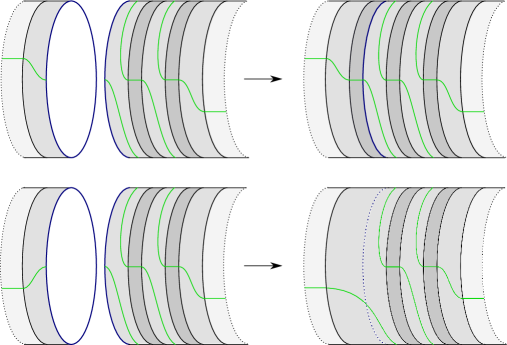
Figure 4. The standard representatives $\phi_{\pm}$ on the top and bottom, respectively. The fixed annuli are shown in dark gray, and the twist regions in medium gray. Note that $\phi_{+}$ has one more fixed annulus $A$ than $\phi_{-}$.

Suppose next that we are in the second case provided by Lemma 2.6: that $\partial S\subset\partial S_{0}$, $\alpha_{0}=\operatorname{id}$, and every boundary component of $S_{0}$ besides $\partial S$ abuts a positive twist region for $\alpha$. Since we are assuming for the proposition that $h$ is not isotopic to the identity, $S_{0}$ must indeed have boundary components other than $\partial S$. Note that $\partial S$ abuts a positive twist region for $\phi_{+}$ and a negative twist region for $\phi_{-}$. Thus, $\partial S_{0}$ has no negative components for $\phi_{+}$, but has both positive and negative components for $\phi_{-}$. It follows that the fixed component $S_{0}$ contributes

$$\dim H_{*}(S_{0};\mathbb{F})$$

to the term

$$\dim H_{*}(\Sigma_{a},\partial_{-}\Sigma_{a};\mathbb{F})$$

for $\dim\mathit{HF}^{symp}(h\cup g_{+})$ in Theorem 2.8 (see Remark 2.9, with $\partial_{-}S_{0}=\emptyset$), but only

$$\dim H_{*}(S_{0},\partial S;\mathbb{F})=\dim H_{*}(S_{0};\mathbb{F})-2$$

to $\dim\mathit{HF}^{symp}(h\cup g_{-})$. The remaining contributions to $\dim\mathit{HF}^{symp}(h\cup g_{\pm})$ are the same, proving the formula in the proposition in this case as well.

We have so far proven the only if direction of the proposition. For the if direction (which, as mentioned above, we do not need for our main theorem or its applications), suppose that $h$ is not right-veering. We must show that

$$\dim\mathit{HF}^{symp}(h\cup g_{+})\neq 2+\dim\mathit{HF}^{symp}(h\cup g_{-}).$$

By Lemma 2.6, $\partial S$ does not abut a positive twist region for $\alpha$. If $\partial S$ abuts a negative twist region, then the inverse of $h$ is right-veering by Lemma 2.6, and we have, by the calculation above and the fact that the dimension of symplectic Floer homology is invariant under taking inverses (see Remark 2.10), that

$$\dim\mathit{HF}^{symp}(h\cup g_{+})=-2+\dim\mathit{HF}^{symp}(h\cup g_{-})\neq 2+\dim\mathit{HF}^{symp}(h\cup g_{-}),$$

as desired.

If $\partial S$ does not abut a negative twist region, then it does not abut a twist region at all, and we have that $\partial S\subset\partial S_{0}$. In this case, Lemma 2.6 says that either $\alpha_{0}\neq\operatorname{id}$, or else $\alpha_{0}=\operatorname{id}$ and some component of $\partial S_{0}\setminus\partial S$ does not abut a positive twist region for $\alpha$. Suppose first that $\alpha_{0}\neq\operatorname{id}$. Then, in the notation of Theorem 2.8, $S_{0}$ belongs to either $\Sigma_{1}$ (the non-fixed periodic components) or $\Sigma_{2}$ (the pseudo-Anosov components). In this case, all regions contribute the same amount to both of $\dim\mathit{HF}^{symp}(h\cup g_{\pm})$, by Theorem 2.8, and

$$\dim\mathit{HF}^{symp}(h\cup g_{+})=\dim\mathit{HF}^{symp}(h\cup g_{-})\neq 2+\dim\mathit{HF}^{symp}(h\cup g_{-}),$$

as desired. Finally, suppose that $\alpha_{0}=\operatorname{id}$ and some component $B$ of $\partial S_{0}\setminus\partial S$ does not abut a positive twist region for $\alpha$. There are three cases to consider.

Case 1: $S_{0}\subset\Sigma_{a}$. Suppose that $S_{0}$ does not abut any pseudo-Anosov components for $\alpha$, so that $S_{0}$ is a component of $\Sigma_{a}$ in the notation of Theorem 2.8. Let

$$\alpha^{\prime}=\alpha|_{S\setminus\textrm{int}(S_{0})}.$$

We claim that $B$ must abut a negative twist region. Otherwise, $B$ does not abut any twist region, and therefore abuts a periodic component for $\alpha^{\prime}$. Moreover, $c_{B}(\alpha^{\prime})=0$. This implies by Lemma 2.5 that $\alpha^{\prime}$ restricts to the identity on this component. But that contradicts the minimality of the invariant set for $\alpha$, since $\alpha_{0}=\operatorname{id}$ as well. Thus, $B$ abuts a negative twist region. As before, $\partial S$ abuts a positive twist region for $\phi_{+}$ and a negative twist region for $\phi_{-}$. Therefore, $\partial S_{0}$ has both positive and negative boundary components for $\phi_{+}$, from which it follows by Remark 2.9 that the fixed component $S_{0}$ contributes

$$\dim H_{*}(S_{0};\mathbb{F})-2$$

to the term

$$\dim H_{*}(\Sigma_{a},\partial_{-}\Sigma_{a};\mathbb{F})$$

for $\dim\mathit{HF}^{symp}(h\cup g_{+})$ in Theorem 2.8. Moreover, $S_{0}$ contributes at least

$$\dim H_{*}(S_{0};\mathbb{F})-2$$

to $\dim\mathit{HF}^{symp}(h\cup g_{-})$. The remaining contributions to $\dim\mathit{HF}^{symp}(h\cup g_{\pm})$ are the same for both, proving that

$$\dim\mathit{HF}^{symp}(h\cup g_{+})\leq\dim\mathit{HF}^{symp}(h\cup g_{-})<2+\dim\mathit{HF}^{symp}(h\cup g_{-}),$$

as desired.

Case 2: $S_{0}\subset\Sigma_{b,p}$. Suppose that $S_{0}$ abuts exactly one pseudo-Anosov component for $\alpha$, meeting $\partial S_{0}$ in $p$ prongs (note that it does not abut a pseudo-Anosov component for $\beta_{\pm}$), so that $S_{0}$ is a component of $\Sigma_{b,p}$ in the notation of Theorem 2.8. Let $\mathring{S_{0}}$ be the complement of an open disk in $S_{0}$. Then, by the conventions in §2.3, $\partial_{-}S_{0}$ is a nonempty proper subset of $\partial\mathring{S_{0}}$ for both $\phi_{\pm}$. It follows that $S_{0}$ contributes

$$\dim H_{*}(\mathring{S_{0}};\mathbb{F})-2$$

to the term

$$\dim H_{*}(\Sigma_{b,p}^{\circ},\partial_{-}\Sigma_{b,p};\mathbb{F})$$

in Theorem 2.8 for both $\dim\mathit{HF}^{symp}(h\cup g_{\pm})$. The remaining contributions to both dimensions are the same, proving that

$$\dim\mathit{HF}^{symp}(h\cup g_{+})=\dim\mathit{HF}^{symp}(h\cup g_{-})\neq 2+\dim\mathit{HF}^{symp}(h\cup g_{-}),$$

as desired.

Case 3: $S_{0}\subset\Sigma_{c,q}$. Suppose that $S_{0}$ abuts at least two pseudo-Anosov components for $\alpha$, meeting $\partial S_{0}$ in a total of $q$ prongs, so that $S_{0}$ is a component of $\Sigma_{c,q}$ in the notation of Theorem 2.8. Then, by the conventions in §2.3, $\partial_{-}{S_{0}}$ is a nonempty proper subset of $\partial{S_{0}}$ for both $\phi_{\pm}$. It follows that $S_{0}$ contributes

$$\dim H_{*}({S_{0}};\mathbb{F})-2$$

to the term

$$\dim H_{*}(\Sigma_{c,q},\partial_{-}\Sigma_{c,q};\mathbb{F})$$

in Theorem 2.8 for both $\dim\mathit{HF}^{symp}(h\cup g_{\pm})$. The remaining contributions to both dimensions are the same, proving that

$$\dim\mathit{HF}^{symp}(h\cup g_{+})=\dim\mathit{HF}^{symp}(h\cup g_{-})\neq 2+\dim\mathit{HF}^{symp}(h\cup g_{-}),$$

as desired. This completes the proof of the proposition. ∎

Proof of Theorem 1.3.

Suppose that $K\subset Y$ is a fibered knot with right-veering monodromy $h:S\to S$. If $h\sim\operatorname{id}$, then $K$ supports the Stein-fillable contact structure on

$$Y\cong\#^{2g(S)}(S^{1}\times S^{2}),$$

which has nontrivial contact invariant. Therefore, $b(K)>1$, as desired.

Let us now suppose that $h\not\sim\operatorname{id}$, and let us assume for a contradiction that $b(K\subset Y)=1$. Since $h$ is right-veering and $h\not\sim\operatorname{id}$, the monodromy $h^{-1}$ of the mirror $K\subset-Y$ is not right-veering. Thus, $b(K\subset-Y)=1$ by Theorem 1.2. Moreover, $K$ is nontrivial since $h\not\sim\operatorname{id}$. Proposition 3.4 therefore implies that

$$\dim\mathit{HF}^{+}(Z_{0}(J_{+}),\mathrm{top}{-}1)=\dim\mathit{HF}^{+}(Z_{0}(J_{-}),\mathrm{top}{-}1),$$

where $J_{\pm}=K\#L_{\pm}$ and $Z=Y\#(S^{1}\times S^{2})$. Since $Z_{0}(J_{\pm})$ is the mapping torus of $h\cup g_{\pm}$, and $g(S\cup F)\geq 3$, we have by Theorem 2.11 that

$$\mathit{HF}^{+}(Z_{0}(J_{\pm}),\textrm{top}{-}1)\cong\mathit{HF}^{symp}(h\cup\phi_{\pm}).$$

Therefore,

$$\dim\mathit{HF}^{symp}(h\cup\phi_{+})=\dim\mathit{HF}^{symp}(h\cup\phi_{-}).$$

But this contradicts the conclusion of Proposition 4.1. ∎

Proof of Corollary 1.5.

This follows immediately from Theorems 1.1 and 1.3. ∎

Proof of Corollary 1.7.

As noted in Remark 2.12, $\tau(K)$ is equal to the Alexander grading of the generator of the $E_{\infty}\cong\mathbb{F}$ page of the spectral sequence

$$E_{1}\cong\widehat{\mathit{HFK}}(S^{3},K)\implies\widehat{\mathit{HF}}(S^{3})\cong E_{\infty}.$$

The thinness hypothesis implies that this spectral sequence collapses at the $E_{2}$ page, as noted in Remark 2.14. Thus, every element in the knot Floer homology of $K$ in Alexander grading different from $\tau(K)$ is either 1) a boundary or 2) not a cycle with respect to the $d_{1}$ differential in the spectral sequence. In particular, since $g:=g(K)\neq\tau(K)$, there is a nontrivial component of $d_{1}$ from

$$\widehat{\mathit{HFK}}(S^{3},K,g)\to\widehat{\mathit{HFK}}(S^{3},K,g-1)$$

By Remark 1.4, this implies that $b(K\subset S^{3})=1$. The same reasoning applied to the mirror shows that $b(K\subset-S^{3})=1$ as well. By Theorem 1.3, the monodromies $h^{\pm 1}$ of $K\subset\pm S^{3}$ are thus non-right-veering. In particular, $h$ is neither right-veering nor left-veering. ∎

Proof of Corollary 1.9.

The inequality $|\tau(K)|<g(K)$ means that $K\subset S^{3}$ is nontrivial, and Corollary 1.7 says that the monodromy of $K$ is neither right-veering nor left-veering. Then $K$ is persistently foliar by [DR21, Theorem 1.4]; we note that the cited theorem is really a slight generalization of [Rob01, Theorem 4.7 (1)], which is stated using different terminology and only for pseudo-Anosov monodromy. ∎

Proof of Corollary 1.11.

Suppose $K\subset S^{3}$ is a fibered alternating knot. First, let us suppose that $K$ is a connected sum of torus knots of the form

$$K=T_{2,2n_{1}+1}\,\#\,\dots\,\#\,T_{2,2n_{k}+1}.$$

If $k=1$ and $r$ is a rational number other than $2(2n_{1}+1),$ then $S^{3}_{r}(K)$ is a Seifert manifold with base $S^{2}$. Such manifolds admit co-orientable taut foliations if and only if they are non-L-spaces by [LS07, Theorem 1.1]. For $k=1$ and $r=2(2n_{1}+1)$, $S^{3}_{r}(K)$ is a connected sum of lens spaces and therefore an L-space, and it does not admit a taut foliation since it is reducible. If $k>1$, then $K$ does not admit an L-space surgery by [Krc15, Theorem 1.2], and is persistently foliar by [DR21, Theorem 6.1]. So, in this case, $S^{3}_{r}(K)$ is a non-L-space and admits a co-oriented taut foliation for every $r\in\mathbb{Q}$.

If $K$ is not a connected sum of torus knots, then neither $K$ nor its mirror is strongly quasipositive by [Ni21b, Proposition 3.7]. Thus, $K$ does not admit an L-space surgery, and

$$|\tau(K)|<g(K)$$

[Hed10]. The latter implies by Corollary 1.9 that $K$ is persistently foliar. So, in this case, $S^{3}_{r}(K)$ is a non-L-space and admits a co-oriented taut foliation for every $r\in\mathbb{Q}$. ∎

Proof of Corollary 1.12.

Suppose first that $\tau(K)=g(K)$. From the interpretation of $\tau(K)$ in Remark 2.12 as the Alexander grading of the $E_{\infty}\cong\mathbb{F}$ page of the spectral sequence

$$E_{1}\cong\widehat{\mathit{HFK}}(S^{3},K)\implies\widehat{\mathit{HF}}(S^{3})\cong E_{\infty},$$

we conclude that the generator of $\widehat{\mathit{HFK}}(S^{3},K,g)$ must survive in this spectral sequence. In particular, the component of the $d_{1}$ spectral sequence differential from

$$\widehat{\mathit{HFK}}(S^{3},K,g)\to\widehat{\mathit{HFK}}(S^{3},K,g-1)$$

vanishes. Per Remark 1.4, this implies that $b(K)>1$, which implies by Theorem 1.3 that the monodromy of $K$ is right-veering. Then [Ni20a, Theorem 1.1] says that $0\leq r\leq 4g(K)$.

Suppose next that $\tau(K)=-g(K)$. The fact that $S^{3}_{r}(K)$ is non-hyperbolic implies that

$$S^{3}_{-r}(\overline{K})\cong-S^{3}_{r}(K)$$

is also non-hyperbolic. Since

$$\tau(\overline{K})=-\tau(K)=g(K)=g(\overline{K}),$$

we have by the previous case that $0\leq-r\leq 4g(K)$, which implies that $-4g(K)\leq r\leq 0$.

Finally, if $|\tau(K)|<g(K)$ and the knot Floer homology of $K$ is thin, then Corollary 1.7 tells us that the monodromy of $K$ is neither right-veering nor left-veering. Then [Ni20a, Theorem 1.1] says that $|q|\leq 2$. ∎

References

- [BDL+21] John A. Baldwin, Nathan Dowlin, Adam Simon Levine, Tye Lidman, and Radmila Sazdanovic. Khovanov homology detects the figure-eight knot. Bull. Lond. Math. Soc., 53(3):871–876, 2021.
- [BHS21] John A. Baldwin, Ying Hu, and Steven Sivek. Khovanov homology and the cinquefoil. arXiv:2105.12102, 2021.
- [BS22] John A. Baldwin and Steven Sivek. Khovanov homology detects the trefoils. Duke Math. J., 171(4):885–956, 2022.
- [BVV18] John Baldwin and David Shea Vela-Vick. A note on the knot Floer homology of fibered knots. Algebr. Geom. Topol., 18(6):3669–3690, 2018.
- [CC09] Andrew Cotton-Clay. Symplectic Floer homology of area-preserving surface diffeomorphisms. Geom. Topol., 13(5):2619–2674, 2009.
- [CL] J. C. Cha and C. Livingston. KnotInfo: Table of Knot Invariants. http://www.indiana.edu/~knotinfo. August 30, 2019.
- [DR] Charles Delman and Rachel Roberts. Nontorus alternating knots are persistently foliar. Forthcoming.
- [DR21] Charles Delman and Rachel Roberts. Persistently foliar composite knots. Algebr. Geom. Topol., 21(6):2761–2798, 2021.
- [Eli89] Y. Eliashberg. Classification of overtwisted contact structures on -manifolds. Invent. Math., 98(3):623–637, 1989.
- [Hed05] Matthew Hedden. On knot Floer homology and cabling. Algebr. Geom. Topol., 5:1197–1222, 2005.
- [Hed10] Matthew Hedden. Notions of positivity and the Ozsváth-Szabó concordance invariant. J. Knot Theory Ramifications, 19(5):617–629, 2010.
- [HKK+19] Diana Hubbard, Keiko Kawamuro, Feride Ceren Kose, Olga Plamenevskaya, Katherine Raoux, Linh Truong, and Hannah Turner. Braids, fibered knots, and concordance questions. arXiv:2004.07445, 2019.
- [HKM07] Ko Honda, William H. Kazez, and Gordana Matić. Right-veering diffeomorphisms of compact surfaces with boundary. Invent. Math., 169(2):427–449, 2007.
- [JG93] Bo Ju Jiang and Jian Han Guo. Fixed points of surface diffeomorphisms. Pacific J. Math., 160(1):67–89, 1993.
- [KLT20] Çağatay Kutluhan, Yi-Jen Lee, and Clifford Henry Taubes. , I: Heegaard Floer homology and Seiberg-Witten Floer homology. Geom. Topol., 24(6):2829–2854, 2020.
- [KR13] William H. Kazez and Rachel Roberts. Fractional Dehn twists in knot theory and contact topology. Algebr. Geom. Topol., 13(6):3603–3637, 2013.
- [Krc15] David Krcatovich. The reduced knot Floer complex. Topology Appl., 194:171–201, 2015.
- [LS07] Paolo Lisca and András I. Stipsicz. Ozsváth-Szabó invariants and tight contact 3-manifolds. III. J. Symplectic Geom., 5(4):357–384, 2007.
- [LT12] Yi-Jen Lee and Clifford Henry Taubes. Periodic Floer homology and Seiberg-Witten-Floer cohomology. J. Symplectic Geom., 10(1):81–164, 2012.
- [MO08] Ciprian Manolescu and Peter Ozsváth. On the Khovanov and knot Floer homologies of quasi-alternating links. In Proceedings of Gökova Geometry-Topology Conference 2007, pages 60–81. Gökova Geometry/Topology Conference (GGT), Gökova, 2008.
- [Ni20a] Yi Ni. Exceptional surgeries on hyperbolic fibered knots. arXiv:2007.11774, 2020.
- [Ni20b] Yi Ni. Property G and the 4-genus. arXiv:2007.03721, 2020.
- [Ni21a] Yi Ni. A note on knot Floer homology and fixed points of monodromy. arXiv:2106.03884, 2021.
- [Ni21b] Yi Ni. A Characterization of among Alternating Knots. Acta Math. Sin. (Engl. Ser.), 37(12):1841–1846, 2021.
- [Ni22] Yi Ni. Knot Floer homology and fixed points. arXiv:2201.10546, 2022.
- [OS04] Peter Ozsváth and Zoltán Szabó. Holomorphic disks and knot invariants. Adv. Math., 186(1):58–116, 2004.
- [OS05] Peter Ozsváth and Zoltán Szabó. Heegaard Floer homology and contact structures. Duke Math. J., 129(1):39–61, 2005.
- [OS08] Peter S. Ozsváth and Zoltán Szabó. Knot Floer homology and integer surgeries. Algebr. Geom. Topol., 8(1):101–153, 2008.
- [Rob01] Rachel Roberts. Taut foliations in punctured surface bundles. II. Proc. London Math. Soc. (3), 83(2):443–471, 2001.
- [Sei02] Paul Seidel. Symplectic Floer homology and the mapping class group. Pacific J. Math., 206(1):219–229, 2002.
- [Thu88] William P. Thurston. On the geometry and dynamics of diffeomorphisms of surfaces. Bull. Amer. Math. Soc. (N.S.), 19(2):417–431, 1988.