Spin functional renormalization group for dimerized quantum spin systems

Abstract

We investigate dimerized quantum spin systems using the spin functional renormalization group approach proposed by Krieg and Kopietz [Phys. Rev. B 99, 060403(R) (2019)] which directly focuses on the physical spin correlation functions and avoids the representation of the spins in terms of fermionic or bosonic auxiliary operators. Starting from decoupled dimers as initial condition for the renormalization group flow equations, we obtain the spectrum of the triplet excitations as well as the magnetization in the quantum paramagnetic, ferromagnetic, and thermally disordered phases at all temperatures. Moreover, we compute the full phase diagram of a weakly coupled dimerized spin system in three dimensions, including the correct mean field critical exponents at the two quantum critical points.

I Introduction

Dimerized spin systems are quantum Heisenberg magnets where a dominant antiferromagnetic interaction between two neighboring spins, which form a dimer unit, enforces a singlet ground state at small magnetic fields [1, 2, 3]. The system is then a quantum paramagnet which does not exhibit long-range magnetic order. Low-energy excitations above this ground state can be viewed as gapped bosonic quasiparticles whose density can be controlled by the external magnetic field $H$. As the magnetic field increases, these excitations undergo two separate Bose-Einstein condensation (BEC) quantum phase transitions: in $D=3$ spatial dimensions the first transition is characterized by the emergence of $XY$ antiferromagnetic order at a critical field $H_{c1}$. When the magnetic field is further increased, there is a second transition at $H=H_{c2}$ to a fully polarized ferromagnetic state. These BEC quantum phase transitions and the associated intrinsic quantum fluctuations of dimerized quantum spin systems have attracted considerable interest in recent years, both experimentally and theoretically [4, 5, 6, 1, 7, 11, 8, 9, 10, 2, 12, 14, 13, 3, 15]. Prominent materials which have been shown to be well described by quantum dimer models include ${\rm TlCuCl}_{3}$ [4, 6, 18, 19, 16, 1, 7, 8, 20, 10, 15], ${\rm KCuCl}_{3}$ [17, 5, 19], and ${\rm BaCuSi}_{2}{\rm O}_{6}$ [21, 11, 12, 14, 13], among many others [3].

The basic features of the phase diagram of dimerized quantum spin systems have already been revealed in $1970$ via mean-field theory [22]. However, in several respects the mean-field results compare poorly with experiments. For example, mean-field theory fails to reproduce the power law behavior of the critical temperature that is expected for the BEC quantum phase transition and has been observed experimentally [4, 6, 7, 9, 12, 3, 15]. Another drawback of this mean-field approach is that it does not directly deal with the physical spin operators but with auxiliary spin-$1/2$ operators which capture only the two lowest states of the dimer. While this reduction of the Hilbert space allows for a simple mean-field description of the quantum paramagnetic phase, it breaks down at elevated temperatures, where the higher states cannot be neglected, as well as for small magnetic fields, where the Zeeman splitting between the excited states becomes small. A more sophisticated method to study dimerized spin systems is based on the representation of the spin operators in terms of suitably defined auxiliary bosons [4, 16, 11, 8, 20, 10, 13, 3, 15]. However, this strategy also has some disadvantages: first of all, the mapping to auxiliary Bose operators obscures the direct connection to the physical spin operators which tends to obscure the physical interpretation of the results. Moreover, the Hilbert space of the Bose operators contains unphysical states which should be eliminated by means of some projection procedure, such as an infinite on-site repulsion. At elevated temperatures, one furthermore has to account for the thermal reweighting of the dimer states by an appropriate ansatz [10].

In this work, we study dimerized quantum spin systems using the functional renormalization group (FRG) approach to quantum spin systems recently developed in Refs. [23, 24, 25, 26, 27, 28]. Our spin FRG approach generalizes and extends earlier work by Machado and Dupuis [29] who developed a lattice FRG group approach for classical spin systems. Although later the lattice FRG was also used to study bosonic quantum lattice models [30, 31, 32, 33, 34], the direct application of this method to quantum spin systems was not possible due to some technical difficulties related to the existence of the average effective action of quantum Heisenberg models with spin-rotational invariance. In Refs. [23, 24, 25, 26, 27, 28] we have developed several strategies to avoid these technical difficulties. In contrast to methods based on auxiliary bosons [4, 16, 11, 8, 20, 10, 13, 3, 15], our spin FRG directly manipulates the physical spin correlation functions, thus circumventing all issues associated with the expression of quantum spins in terms of bosonic or fermionic auxiliary degrees of freedom. We show in particular that a straightforward truncation of the spin FRG flow equations yields good results for the excitation spectrum and thermodynamics of weakly coupled dimers outside of the antiferromagnetic $XY$ phase at all temperatures and magnetic fields, including the critical fields where the system exhibits BEC quantum phase transitions. We also obtain the correct (mean field) critical exponents at the BEC quantum critical points in dimension $D=3$, and compute corrections to the lower critical field due to quantum fluctuations.

The rest of this work is organized as follows: In Sec. II we define a model Hamiltonian for a dimerized quantum spin system and discuss its phase diagram qualitatively. In Sec. III, we then formulate the spin FRG for our dimerized quantum spin systems, develop a truncation strategy for the flow equations, and present our FRG results for the mode spectrum and the phase diagram. Finally, in Sec. IV we conclude with a summary of our main results and an outlook on future research directions. In two appendices we give additional technical details: in Appendix A we explicitly give the imaginary-time-ordered spin correlation functions of a single dimer involving up to four spins which are needed to calculate the initial values of the vertices in our spin FRG flow equations. Appendix B contains a brief description of our spin FRG formalism.

II Dimerized quantum spin systems

The essential physics of dimerized quantum spin systems is described by the following quantum Heisenberg spin Hamiltonian,

$${\cal H}={} \frac{1}{2}\sum_{ij}\sum_{nm=1}^{2}\left(J_{ij,nm}^{\bot}\bm{s}_{i,n}^{\bot}\cdot\bm{s}_{j,m}^{\bot}+J_{ij,nm}^{\parallel}s_{i,n}^{z}s_{j,m}^{z}\right)$$

$$+A\sum_{i}\bm{s}_{i,1}\cdot\bm{s}_{i,2}-H\sum_{i}\sum_{n=1}^{2}s_{i,n}^{z}.$$ (1)

Here, $\bm{s}_{i,n}=(s_{i,n}^{x},s_{i,n}^{y},s_{i,n}^{z})=(\bm{s}_{i,n}^{\bot},s_{i,n}^{z})$ are spin-$1/2$ operators associated with dimer $i=1,\ldots,N$ at magnetic site $n=1,2$. The dimers are coupled antiferromagnetically via the inter-dimer exchange couplings $J_{ij,nm}^{\alpha}>0$ (where $\alpha=\bot,\parallel$), which are assumed to be small compared to the antiferromagnetic intra-dimer exchange $A>0$. Lastly, $H$ is the Zeeman energy associated with an external magnetic field in $z$ direction. Such a system is illustrated schematically in the inset of Fig. 1.

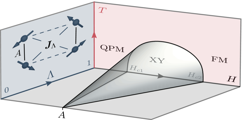
Figure 1: Schematic depiction of the phase diagram of a dimerized spin system as a function of the FRG deformation parameter $\Lambda$. At the beginning of the flow (where $\Lambda=0$ and ${\bf{J}}_{\Lambda=0}=0$) the dimers are completely decoupled. Then the $T=0$ phase diagram consists only of the quantum paramagnetic (QPM) and the ferromagnetic (FM) phase, separated by a quantum critical point at $H=A$. When the inter-dimer exchange couplings ${\bf J}_{\Lambda}$ are turned on with increasing deformation parameter $\Lambda$, this quantum critical point grows into an additional phase exhibiting antiferromagnetic $XY$ ordering in $D=3$ dimensions. The new quantum critical points at the critical fields $H_{c1}$ and $H_{c2}$ respectively separate the QPM and FM phases from the $XY$ phase. Inset: Visualization of a pair of spin dimers, with intra-dimer exchange $A$ and (deformed) inter-dimer exchange couplings ${\bf J}_{\Lambda}$.

Introducing the total and staggered dimer spin operators as

$$\bm{S}_{i}={} \bm{s}_{i,1}+\bm{s}_{i,2},$$ (2a)

$$\bm{T}_{i}={} \bm{s}_{i,1}-\bm{s}_{i,2},$$ (2b)

respectively, we can rewrite the Hamiltonian (1) as

$${\cal H}={\cal H}_{0}+{\cal V}+{\rm const},$$ (3)

where

$${\cal H}_{0}={} \sum_{i=1}^{N}h_{i},$$ (4a)

$$h_{i}={} \frac{A}{2}\bm{S}_{i}^{2}-HS_{i}^{z}$$ (4b)

is the Hamiltonian of a collection of $N$ decoupled dimers, and

$${\cal V}={} \frac{1}{2}\sum_{ij}\left(J_{T,ij}^{\bot}\bm{T}_{i}^{\bot}\cdot\bm{T}_{j}^{\bot}+J_{T,ij}^{\parallel}T_{i}^{z}T_{j}^{z}\right.$$

$$\phantom{\frac{1}{2}\sum_{ij}}+\left.J_{S,ij}^{\bot}\bm{S}_{i}^{\bot}\cdot\bm{S}_{j}^{\bot}+J_{S,ij}^{\parallel}S_{i}^{z}S_{j}^{z}\right)$$ (5)

describes the exchange interactions between the dimers. Note that by writing down the exchange Hamiltonian (II), we have assumed for simplicity that the two magnetic sites of a given dimer are equivalent, such that $J_{ij,11}^{\alpha}=J_{ij,22}^{\alpha}$. The relevant exchange couplings for $\alpha=\bot,\parallel$ are then given by

$$J_{S,ij}^{\alpha}={} \frac{1}{2}\left(J_{ij,11}^{\alpha}+J_{ij,12}^{\alpha}\right),$$ (6a)

$$J_{T,ij}^{\alpha}={} \frac{1}{2}\left(J_{ij,11}^{\alpha}-J_{ij,12}^{\alpha}\right).$$ (6b)

For inequivalent magnetic sites, there is an additional $\bm{S}_{i}\cdot\bm{T}_{j}$ exchange coupling. However, we will see below that for weakly coupled dimers at low energies, this additional coupling does not give rise to relevant interaction processes because the dynamics of the total and staggered spin operators are well separated in energy.

Before proceeding further, it is instructive to consider the Hamiltonian (4b) of a single dimer in more detail. Its eigenstates are given by the singlet state

$$\ket{s}_{i}=\frac{1}{\sqrt{2}}\left(\ket{\uparrow\downarrow}_{i}-\ket{\downarrow\uparrow}_{i}\right),$$ (7)

and the three Zeeman-split triplet states,

$$\ket{t+}_{i} =\ket{\uparrow\uparrow}_{i},$$ (8a)

$$\ket{t0}_{i} =\frac{1}{\sqrt{2}}\left(\ket{\uparrow\downarrow}_{i}+\ket{\downarrow\uparrow}_{i}\right),$$ (8b)

$$\ket{t-}_{i} =\ket{\downarrow\downarrow}_{i}.$$ (8c)

The corresponding eigenenergies are

$$E^{s}={} 0,$$ (9a)

$$E^{+}={} A-H,$$ (9b)

$$E^{0}={} A,$$ (9c)

$$E^{-}={} A+H.$$ (9d)

From these energies it is obvious that at the magnetic field $H=A$ an isolated dimer exhibits at zero temperature a quantum phase transition from the singlet state, which is a quantum paramagnet, to the fully polarized $+$ triplet state. At finite temperatures $T=1/\beta>0$ the four dimer states are thermally occupied, with Boltzmann factors

$$p^{0}={} p^{s}e^{-\beta E^{0}},$$ (10a)

$$p^{\pm}={} p^{s}e^{-\beta E^{\pm}},$$ (10b)

$$p^{s}={} \frac{1}{1+e^{-\beta E^{+}}+e^{-\beta E^{0}}+e^{-\beta E^{-}}}.$$ (10c)

These Boltzmann factors and the associated eigenenergies fully determine all correlation functions of the single dimer. It turns out that with our truncation of the FRG flow equations we need time-ordered single-dimer correlation functions involving up to four powers of the spin operators. In spite of the simplicity of the single-dimer Hamiltonian, these correlation functions have a highly non-trivial frequency dependence. We summarize the relevant expressions in Appendix A.

The inter-dimer exchange ${\cal{V}}$ in Eq. (II) has a two-fold effect on the properties of a single dimer: firstly, it endows the eigenenergies (9) with a dispersion, and secondly, it enables interaction between the different eigenstates of the isolated dimer. This also leads to the emergence of a new phase at the quantum critical point $H=A$ of the isolated dimer: in dimension $D=3$, this phase exhibits XY antiferromagnetic long-range order as indicated in Fig. 1, while in $D=2$ and $D=1$ it corresponds to a Berezinskii-Kosterlitz-Thouless or a Luttinger liquid phase, respectively [3].

III FRG Flow equations for dimerized quantum spin systems

III.1 Spin FRG

The spin FRG approach proposed in Ref. [23] and further developed in Refs. [24, 25, 26, 27, 28] is based on a formally exact renormalization group flow equation for the generating functional of connected spin correlation functions. As such, it does not require projecting the physical spin operators onto auxiliary bosons or fermions with restricted Hilbert spaces. In fact, the spin FRG combines the old spin-diagram technique developed by Vaks, Larkin and Pikin [35, 36, 37] with modern FRG methods [38, 39, 40, 41, 42, 43]. It turns out that the spin FRG flow equation is formally equivalent to the bosonic Wetterich equation [23], which allows us to utilize the established diagrammatic FRG techniques for bosons [41], thus avoiding the more complicated diagrammatic rules of the spin diagram technique [35, 36, 37] . The non-trivial $SU(2)$ algebra of the spin operators is taken into account via non-trivial initial conditions for the flow equations.

To set up the spin FRG in the context of our dimerized spin system (1), we replace the inter-dimer exchange couplings $J_{a,ij}^{\alpha}$ (where $a=S,T$) by deformed couplings $J_{\Lambda,a,ij}^{\alpha}$. Here, the continuous parameter $\Lambda\in[0,1]$ plays the role of the flowing cutoff in the FRG. The deformed couplings $J_{\Lambda,a,ij}^{\alpha}$ are to be chosen such that $J_{\Lambda=1,a,ij}^{\alpha}=J_{a,ij}^{\alpha}$, while for $\Lambda=0$ the model should be simple enough to allow for a controlled solution. For a dimerized spin system, a natural choice is $J_{\Lambda=0,a,ij}^{\alpha}=0$. In this case, the Hamiltonian at the initial scale is given by the Hamiltonian (4) of decoupled dimers, which is exactly solvable and already contains information on both the quantum disordered state at low magnetic fields and temperatures as well as on the quantum phase transition to the ferromagnetic state at elevated magnetic fields; see Appendix A. The phase diagram resulting from this flow is schematically depicted in Fig. 1.

In the following, we will consider the FRG flow of a special hybrid functional $\Gamma_{\Lambda}[\varphi]$ which generates irreducible vertices with the following properties: the vertices should be (a) one-line irreducible with respect to all three components of the staggered spin propagators; (b) one-line irreducible with respect to the two transverse components of the total spin propagators; and (c) the vertices should be interaction-irreducible with respect to cutting a longitudinal inter-dimer interaction between the total spins. The explicit construction of a functional $\Gamma_{\Lambda}[\varphi]$ with these properties has been discussed in Refs. [25, 27] and is reviewed in Appendix B. At imaginary time $\tau$, the superfield $\varphi_{a,i}^{\alpha}(\tau)$ then corresponds for $a=S$ and $\alpha=x,y$ to the local transverse magnetization, for $a=S$ and $\alpha=z$ to the the fluctuating part of the local inter-dimer longitudinal exchange field, and for $a=T$ and $\alpha=x,y,z$ to the three components the local staggered spin. The six components of the superfield $\varphi=(\varphi_{a,i}^{\alpha}(\tau))$, where the flavor index $a=S,T$ refers to the total and the staggered spin of a given dimer, are then explicitly given by

$$(\varphi_{a,i}^{\alpha}(\tau))=\left(\begin{array}[]{c}\varphi_{S,i}^{x}(\tau)\\ \varphi_{S,i}^{y}(\tau)\\ \varphi_{S,i}^{z}(\tau)\\ \varphi_{T,i}^{x}(\tau)\\ \varphi_{T,i}^{y}(\tau)\\ \varphi_{T,i}^{z}(\tau)\end{array}\right)=\left(\begin{array}[]{c}\langle S_{i}^{x}(\tau)\rangle\\ \langle S_{i}^{y}(\tau)\rangle\\ \varphi_{i}(\tau)\\ \langle T_{i}^{x}(\tau)\rangle\\ \langle T_{i}^{y}(\tau)\rangle\\ \langle T_{i}^{z}(\tau)\rangle\end{array}\right),$$ (11)

where the longitudinal total-spin exchange field $\varphi_{i}(\tau)$ is defined in Appendix B, see also Ref. [25]. The different treatment of the longitudinal total spin of a dimer is necessitated by the $U(1)$ spin-rotational symmetry around the $z$ axis of the Hamiltonian (4) of decoupled dimers at the initial scale, which implies that the longitudinal magnetization field has no dynamics at $\Lambda=0$ when the coupling between the dimers is switched off [25]. For details on the derivation of this functional and the associated flow equations, we refer to Appendix B and to Refs. [23, 25].

For a given value of the deformation parameter $\Lambda$, the vertex expansion of our hybrid generating functional is of the form

$$\Gamma_{\Lambda}[\varphi]={} \beta Nf_{\Lambda}+\int_{K}\sum_{a=S,T}\left[\Gamma_{\Lambda,aa}^{+-}(-K,K)\varphi_{a}^{-}(-K)\varphi_{a}^{+}(K)+\frac{1}{2!}\Gamma_{\Lambda,aa}^{zz}(-K,K)\varphi_{a}^{z}(-K)\varphi_{a}^{z}(K)\right]$$

$$+\int_{K_{1}K_{2}K_{3}}\delta\left(K_{1}+K_{2}+K_{3}\right)\left[\sum_{a=S,T}\Gamma_{\Lambda,aaS}^{+-z}(K_{1},K_{2},K_{3})\varphi_{a}^{-}(K_{1})\varphi_{a}^{+}(K_{2})\varphi_{S}^{z}(K_{3})\vphantom{\frac{1}{3!}}\right.$$

$$\phantom{+}+\Gamma_{\Lambda,TST}^{+-z}(K_{1},K_{2},K_{3})\varphi_{T}^{-}(K_{1})\varphi_{S}^{+}(K_{2})\varphi_{T}^{z}(K_{3})+\Gamma_{\Lambda,STT}^{+-z}(K_{1},K_{2},K_{3})\varphi_{S}^{-}(K_{1})\varphi_{T}^{+}(K_{2})\varphi_{T}^{z}(K_{3})$$

$$\phantom{+}\left.\vphantom{\sum_{s=S,T}}+\frac{1}{2!}\Gamma_{\Lambda,TTS}^{zzz}(K_{1},K_{2},K_{3})\varphi_{T}^{z}(K_{1})\varphi_{T}^{z}(K_{2})\varphi_{S}^{z}(K_{3})+\frac{1}{3!}\Gamma_{\Lambda,SSS}^{zzz}(K_{1},K_{2},K_{3})\varphi_{S}^{z}(K_{1})\varphi_{S}^{z}(K_{2})\varphi_{S}^{z}(K_{3})\right]$$

$$+{\cal O}\left(\varphi^{4}\right),$$ (12)

where $K=(\bm{k},i\omega)$ is a collective label for momentum $\bm{k}$ and Matsubara frequency $i\omega$; the corresponding integration and delta symbols are defined as $\int_{K}=(\beta N)^{-1}\sum_{\bm{k},i\omega}$ and $\delta(K)=\beta N\delta_{\bm{k},0}\delta_{\omega,0}$, respectively. Here $\varphi_{a}^{\pm}=(\varphi_{a}^{x}\pm i\varphi_{a}^{y})/\sqrt{2}$ denote the spherical transverse field components and the field-independent contribution $f_{\Lambda}$ can be identified with the flowing free energy per dimer. Note that in writing down the vertex expansion (12), we already took into account two symmetries of the Hamiltonian (1): the global $U(1)$ spin-rotational symmetry around the $z$ axis that corresponds to spin conservation, as well as the invariance under exchange of the two magnetic sites; i.e., $\bm{s}_{i,1}\leftrightarrow\bm{s}_{i,2}$ or $\bm{T}_{i}\leftrightarrow-\bm{T}_{i}$. The former implies that only vertex functions with the same number of $+$ and $-$ labels are finite, while the latter requires all vertices to have an even number of $T$ labels. In doing so, we have of course neglected the possibility of spontaneous symmetry breaking that is necessary to describe the $XY$ ordered phase of dimerized spin systems in dimension $D=3$ [4, 2, 3]. Although it is possible to extend our spin FRG approach to include also the XY ordering, this is beyond the scope of the present work. The 2-point vertex functions determine the flowing spin propagators via

$$G_{\Lambda,a}^{\bot}(K)={} \frac{1}{\Gamma_{\Lambda,aa}^{+-}(-K,K)+J_{\Lambda,a,\bm{k}}^{\bot}-J_{a,\bm{k}}^{\bot}},$$ (13a)

$$G_{\Lambda,T}^{\parallel}(K)={} \frac{1}{\Gamma_{\Lambda,TT}^{zz}(-K,K)+J_{\Lambda,T,\bm{k}}^{\parallel}-J_{T,\bm{k}}^{\parallel}},$$ (13b)

$$G_{\Lambda,S}^{\parallel}(K)={} \frac{\Pi_{\Lambda}(K)}{1+J_{\Lambda,S,\bm{k}}^{\parallel}\Pi_{\Lambda}(K)},$$ (13c)

where $J_{\Lambda,a,\bm{k}}^{\alpha}$ is the Fourier transform of $J_{\Lambda,a,ij}^{\alpha}$ and

$$\Pi_{\Lambda}(K)=-\Gamma_{\Lambda,SS}^{zz}(-K,K)-\frac{1}{J_{S,\bm{k}}^{\parallel}}$$ (14)

is the interaction-irreducible longitudinal spin susceptibility [25]. The decoupled-dimer initial conditions for these propagators are listed in Eqs. (A8). Note that the propagators (13) are the $2$-spin correlation functions, which directly determine quantities of experimental interest like the dynamical spin structure factor.

For the explicit calculations in this work, we assume that the dimers form a simple cubic lattice in three dimensions with lattice constant $a$, and that all inter-dimer exchange interactions are isotropic. This setup is illustrated in Fig. 2.

Figure 2: Illustration of a simple cubic lattice of dimers (D) in three dimensions. The dimers interact via (deformed) isotropic inter-dimer exchange couplings ${\bf J}_{\Lambda}$. The two spins that form a given dimer interact with each other via the intra-dimer exchange $A$.

Then we can write the flowing exchange couplings as

$$J^{\alpha}_{\Lambda,a,\bm{k}}=J^{\alpha}_{a,\bm{k}=0}\gamma_{\Lambda,\bm{k}},$$ (15)

with $\gamma^{\alpha}_{\Lambda=0,\bm{k}}=0$ and $\gamma^{\alpha}_{\Lambda=1,\bm{k}}=\gamma^{\alpha}_{\bm{k}}$. Here,

$$\gamma_{\bm{k}}=\frac{1}{3}\left[\cos\left(k^{x}a\right)+\cos\left(k^{y}a\right)+\cos\left(k^{z}a\right)\right]$$ (16)

is the nearest neighbor form factor, which satisfies $-1\leq\gamma_{\bm{k}}\leq 1$. For the deformation scheme, we use a Litim regulator [44], given by

$$\gamma_{\Lambda,\bm{k}} ={\rm sgn}\left(\gamma_{\bm{k}}\right)\left.\begin{cases}\Lambda,&\Lambda<\left|\gamma_{\bm{k}}\right|\\ \left|\gamma_{\bm{k}}\right|,&\Lambda\geq\left|\gamma_{\bm{k}}\right|\end{cases}\right\}$$

$$=\gamma_{\bm{k}}-{\rm sgn}\left(\gamma_{\bm{k}}\right)\left(\left|\gamma_{\bm{k}}\right|-\Lambda\right)\Theta\left(\left|\gamma_{\bm{k}}\right|-\Lambda\right),$$ (17)

such that

$$\partial_{\Lambda}\gamma_{\Lambda,\bm{k}}={\rm sgn}\left(\gamma_{\bm{k}}\right)\Theta\left(\left|\gamma_{\bm{k}}\right|-\Lambda\right).$$ (18)

Physically, the flow then corresponds to increasing the bandwidth of all exchange interactions from $0$ to the final value $2$. This deformation scheme has the advantage that closed loop integrations that frequently appear in the spin FRG flow equations can be performed analytically as follows,

$$\int_{\bm{k}}\left(\partial_{\Lambda}\gamma_{\Lambda,\bm{k}}\right)F_{\Lambda}\left(\gamma_{\Lambda,\bm{k}}\right)=n(\Lambda)\left[F_{\Lambda}(\Lambda)-F_{\Lambda}(-\Lambda)\right].$$ (19)

Here, $\int_{\bm{k}}=N^{-1}\sum_{\bm{k}}$, $F_{\Lambda}\left(\gamma_{\Lambda,\bm{k}}\right)$ is an arbitrary function of the deformed exchange coupling, and

$$n(\Lambda)=\int_{\Lambda}^{1}d\epsilon\,\nu(\epsilon)$$ (20)

is an effective number of states between dimensionless energies $\Lambda$ and $1$, with the density of states

$$\nu(\epsilon)=\int_{\bm{k}}\delta\left(\gamma_{\bm{k}}-\epsilon\right)$$ (21)

of the exchange interaction. The two functions $n(\Lambda)$ and $\nu(\epsilon)$ can be computed once for a given structure factor and can then be used subsequently in all flow equations. We stress at this point that the spin FRG approach is applicable to any lattice structure. Different lattices only modify the density of states $\nu(\epsilon)$, without altering the form of the spin FRG flow equations. Here, we consider an isotropic simple cubic lattice both for simplicity and to facilitate a direct comparison to quantum Monte Carlo results in Sec. III.4. For any unfrustrated lattice, we furthermore expect qualitatively similar results.

III.2 Tadpole resummation

At finite magnetic field $H$ and temperature $T$, the system possesses a finite magnetization $M$. In addition to the $n$-point vertex functions, we should then also keep track of the renormalization group flow of the longitudinal inter-dimer exchange field

$$\phi_{\Lambda}=-J_{\Lambda,S,\bm{k}=0}^{\parallel}M_{\Lambda}$$ (22)

which is determined by the flowing magnetization $M_{\Lambda}$. Neglecting for the moment all terms in the flow equations for the irreducible vertices involving loop integrations, we find that the flow of the exchange field generates the following infinite hierarchy of flow equations for the $n$-point vertices with $n\geq 2$ external legs,

$$\partial_{\Lambda}\Gamma_{\Lambda,a_{1}\ldots a_{n}}^{\alpha_{1}\ldots\alpha_{n}}(K_{1},\ldots,K_{n})$$

$$={} \Gamma_{\Lambda,a_{1}\ldots a_{n}S}^{\alpha_{1}\ldots\alpha_{n}z}(K_{1},\ldots,K_{n},0)\partial_{\Lambda}\phi_{\Lambda}.$$ (23)

Graphically, these flow equations correspond to the tadpole diagrams displayed in Fig. 3.

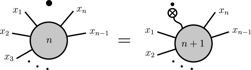
Figure 3: Diagrammatic representation of the tadpole flow equations (23). The filled circles with $n$ external legs represent $n$-point vertices. The labels of each leg are collected into $x_{i}=(\alpha_{i}s_{i}K_{i})$. The crossed circle with a wavy line represents the flowing exchange field $\phi_{\Lambda}$. Dots above one of these elements signify a scale derivative $\partial_{\Lambda}$.

Integrating the tadpole flow equation (23) from $0$ to $\Lambda$ and iterating we obtain the explicit solution

$$\Gamma_{\Lambda,a_{1}\ldots a_{n}}^{\alpha_{1}\ldots\alpha_{n}}(K_{1},\ldots,K_{n})$$

$$={} \sum_{m=0}^{\infty}\frac{\phi_{\Lambda}^{m}}{m!}\Gamma_{0,a_{1}\ldots a_{n}\underbrace{\scriptstyle S\ldots S}_{m}}^{\alpha_{1}\ldots\alpha_{n}\overbrace{\scriptstyle z\ldots z}^{m}}(K_{1},\ldots,K_{n},\overbrace{0,\ldots,0}^{m}).$$ (24)

We now note that by definition of our hybrid functional $\Gamma_{\Lambda}[\varphi]$ given in Eq. (B17) of Appendix B (see also Ref. [25]) the initial vertex functions appearing on the right-hand side of the solution (24) can be related to lower-order vertex functions by taking derivatives with respect to the magnetic field $H$,

$$\Gamma_{0,a_{1}\ldots a_{n}\underbrace{\scriptstyle S\ldots S}_{m}}^{\alpha_{1}\ldots\alpha_{n}\overbrace{\scriptstyle z\ldots z}^{m}}(K_{1},\ldots,K_{n},\overbrace{0,\ldots,0}^{m})$$

$$={} \partial_{H}^{m}\Gamma_{0,a_{1}\ldots a_{n}}^{\alpha_{1}\ldots\alpha_{n}}(K_{1},\ldots,K_{n}).$$ (25)

Therefore we can write the solution (24) of the tadpole flow equation (23) as

$$\Gamma_{\Lambda,a_{1}\ldots a_{n}}^{\alpha_{1}\ldots\alpha_{n}}(K_{1},\ldots,K_{n})$$

$$={} \sum_{m=0}^{\infty}\frac{\phi_{\Lambda}^{m}}{m!}\partial_{H}^{m}\Gamma_{0,a_{1}\ldots a_{n}}^{\alpha_{1}\ldots\alpha_{n}}(K_{1},\ldots,K_{n})$$

$$={} \left.\Gamma_{0,a_{1}\ldots a_{n}}^{\alpha_{1}\ldots\alpha_{n}}(K_{1},\ldots,K_{n})\right|_{H\to H+\phi_{\Lambda}}.$$ (26)

Hence, the resummation of the tadpole diagrams shown in Fig. 3 alone simply yields the mean field shift of the magnetic field

$$H\to H+\phi_{\Lambda}=H-J_{\Lambda,S,\bm{k}=0}^{\parallel}M_{\Lambda}$$ (27)

in all vertex functions. Properly including this shift during the flow proves to be crucial to obtain physically meaningful results in the following calculations.

In a simple truncation where only these tadpole diagrams are taken into account, the flowing staggered spin propagators are given by

$$G_{\Lambda,T}^{\bot}(K)={} \frac{M_{0}\left(i\omega+A-H-\phi_{\Lambda}\right)-2m_{0}A}{\left(E^{+}_{\Lambda,\bm{k}}+i\omega\right)\left(E^{-}_{\Lambda,\bm{k}}-i\omega\right)},$$ (28a)

$$G_{\Lambda,T}^{\parallel}(K)={} \frac{2\left(p^{s}-p^{0}\right)A}{\left(E^{0}_{\Lambda,\bm{k}}+i\omega\right)\left(E^{0}_{\Lambda,\bm{k}}-i\omega\right)},$$ (28b)

where

$$M_{0}=p^{+}-p^{-}$$ (29)

is the magnetic moment of an isolated dimer and

$$m_{0}=p^{+}-p^{s},$$ (30)

where the Boltzmann factors should be evaluated at the flowing magnetic field $H+\phi_{\Lambda}$. Note that $m_{0}$ corresponds to the difference in occupation of the two lowest energy states of an isolated dimer and thus measures whether the dimer is closer to the disordered singlet state or the fully polarized $+$ triplet state. The flowing dispersion relations of the three triplet states are in this approximation given by

$$E^{\pm}_{\Lambda,\bm{k}}={} \sqrt{\left(A+\frac{M_{0}}{2}J_{\Lambda,T,\bm{k}}^{\bot}\right)^{2}-2m_{0}AJ_{\Lambda,T,\bm{k}}^{\bot}}$$

$$\mp\left(\frac{M_{0}}{2}J_{\Lambda,T,\bm{k}}^{\bot}+H+\phi_{\Lambda}\right),$$ (31a)

$$E^{0}_{\Lambda,\bm{k}}={} \sqrt{A^{2}+2\left(p^{s}-p^{0}\right)AJ_{\Lambda,T,\bm{k}}^{\parallel}}.$$ (31b)

Because $M_{0}$ and $m_{0}$ are complicated functions of temperature and (flowing) magnetic field determined by the exact dimer correlation functions, the properties of the triplet modes (31) vary considerably over the phase diagram. In particular, for $T\ll A$ and $H<H_{c1}$ the system is in the quantum paramagnetic regime ($M\approx 0$); in this case we also have $M_{0}\approx 0\approx p^{0}$ and $m_{0}\approx-p^{s}\approx-1$. Then the triplet dispersions (31) reduce at the end of the flow to

$$E_{\bm{k}}^{\pm}\approx{} \sqrt{A^{2}+2AJ_{T,\bm{k}}^{\bot}}\mp H,$$ (32a)

$$E^{0}_{\bm{k}}\approx{} \sqrt{A^{2}+2AJ_{T,\bm{k}}^{\parallel}}.$$ (32b)

in agreement with calculations for dimerized quantum spin systems based on the random-phase approximation [21, 17, 5]. These dispersions are shown in Fig. 4 (a).

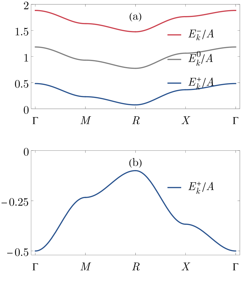
Figure 4: Zero-temperature triplet dispersions for a simple cubic lattice with inter-dimer exchange couplings $J_{T,\bm{k}=0}^{\bot}=J_{T,\bm{k}=0}^{\parallel}=J_{0}=0.2\,A$, for (a) $H=0.7\,A$ in the quantum paramagnetic phase, and (b) $H=1.5\,A$ in the ferromagnetic phase.

It is then easy to see that the gap of the lowest ($+$) triplet dispersion vanishes at the magnetic field

$$H_{c1}=\sqrt{A^{2}+2A{\rm min}_{\bm{k}}J_{T,\bm{k}}^{\bot}}<A,$$ (33)

which gives a first approximation for the lower quantum critical field of the dimerized spin system. This value of the quantum critical field of course still lacks corrections due to quantum fluctuations [9] described by the loop integrations neglected in Eq. (26). In Sec. III.4 we will explicitly calculate the effect of quantum fluctuations on the critical fields.

Another regime where our general expressions (32) simplify is the ferromagnetic phase where $M\approx 1$. Assuming $T\ll A$ and $H>H_{c2}$ we then have $M_{0}\approx 1\approx m_{0}$ and $p^{s}\approx 0\approx p^{0}$. Then the two high-energy triplet modes disappear completely from the propagators (28), so that at the end of the flow we obtain a spin-wave like dispersion for the remaining low-energy mode,

$$E_{\bm{k}}^{+}\approx A-H+J_{S,\bm{k}=0}^{\parallel}-J_{T,\bm{k}}^{\bot};$$ (34)

see Fig. 4 (b). The gap of this mode vanishes at the upper critical field

$$H_{c2}=A+J_{S,\bm{k}=0}^{\parallel}-{\rm min}_{\bm{k}}J_{T,\bm{k}}^{\bot}>A.$$ (35)

Note that at the quantum critical points themselves, the $+$ dispersion in Eq. (32) and Eq. (34) is at long-wavelengths quadratic in $\bm{k}$ for generic inter-dimer exchange couplings. Therefore the dynamical critical exponent is $z=2$, as expected for BEC quantum critical points [3]. When approaching either of the quantum critical fields $i=1,2$ at zero temperature, the gap of the $+$ mode furthermore vanishes as $|H-H_{ci}|$, implying the correlation length critical exponent $\nu=1/z=1/2$ [3].

Next, consider the regime of elevated temperatures (above the antiferromagnetic dome) and for flowing magnetic fields $H+\phi_{\Lambda}\approx A$, that is, in the vicinity of the critical field of the isolated dimer. Then we may approximate $m_{0}\approx 0$ and the flowing dispersion $E_{\Lambda,\bm{k}}^{+}$ of the lowest triplet state vanishes as well. However, since the energy $E_{\Lambda,\bm{k}}^{+}$ also cancels out of the associated propagator (28a), this corresponds to a simple level crossing instead of a phase transition. At this point, this mode changes from a hole-like excitation with $\omega<0$ to a particle-like excitation with $\omega>0$.

It is important to realize that beyond the simple limits discussed above, the flowing triplet dispersions (31) contain information on the entire phase diagram through the Boltzmann factors of the isolated dimer as well as through the flowing magnetization $M_{\Lambda}$. This is similar to the thermal reweighting of the dimer states proposed in Ref. [10]. In particular, the condition that the gap of the lowest $+$ triplet mode vanishes yields an estimate for the full phase transition curve of the antiferromagnetic dome, which will be discussed in Sec. III.3 and in Fig. 6 below.

Lastly, let us also give the flowing transverse total spin propagator and the longitudinal interaction-irreducible total spin susceptibility in the tadpole approximation. The former is given by

$$G_{\Lambda,S}^{\bot}(K)=\frac{M_{0}}{H+\phi_{\Lambda}+M_{0}J_{\Lambda,S,\bm{k}}^{\bot}-i\omega},$$ (36)

while the interaction-irreducible total spin susceptibility is

$$\Pi_{\Lambda}(K)=\delta_{\omega,0}\partial_{H}M_{0}(H+\phi_{\Lambda}).$$ (37)

In the regimes of interest to us the effects of both of these total spin correlation functions on the flow of the other correlation functions can be neglected. To justify this, we note that transverse total spin correlation function is negligible in the quantum paramagnetic phase because $M_{0}\approx 0$, and in the ferromagnetic phase at large magnetic fields because then it only has a single pole at high energies $\sim H$, which is not thermally excited. As far as the longitudinal interaction-irreducible total spin susceptibility in Eq. (37) is concerned, it is only relevant close to the quantum critical point $H=A$ of the isolated dimer, see Appendix A. As this point lies deep in the antiferromagnetic dome where our theory is not applicable in its present form anyway, we may also neglect it.

To conclude this section, let us point out that already on the tadpole level, the spin FRG contains two infinite resummations – self-consistent mean field theory and a random-phase approximation – of the inter-dimer exchange couplings. Both of these are inherently non-perturbative. Thus, any truncation of the spin FRG flow equations goes beyond a simple perturbation expansion in the inter-dimer exchange. While small inter-dimer exchange couplings make the truncation of the spin FRG flow equations at a low loop order a more controlled approximation, such a truncation can consequently also yield reasonable results for larger values of these exchange couplings.

III.3 Thermal fluctuations

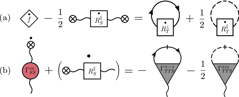
Figure 5: Graphical representation of (a) the flow equation (38) of the free energy and (b) the flow equation (39) of the exchange field. Solid lines with arrows represent the flowing transverse staggered propagator $G_{\Lambda,T}^{\bot}(K)$ and dashed lines the longitudinal staggered propagator $G_{\Lambda,T}^{\parallel}(K)$. An additional slash marks the corresponding single-scale propagator $\dot{G}_{\Lambda,T}^{\alpha}(K)$. The rest of the notation is the same as in Fig. 3.

At finite temperatures, thermodynamic quantities such as the magnetization or the specific heat are expected to be dominated by thermal fluctuations of the dispersive triplet excitations. To take these properly into account, we should include the terms involving loop-integrations on the right-hand sides of the corresponding flow equations. The flow equation for the free energy is

$$\partial_{\Lambda}f_{\Lambda}-\frac{1}{2}\phi_{\Lambda}^{2}\partial_{\Lambda}R_{\Lambda,S,\bm{k}=0}^{\parallel}$$

$$={} \int_{K}G_{\Lambda,T}^{\bot}(K)\partial_{\Lambda}R_{\Lambda,T,\bm{k}}^{\bot}+\frac{1}{2}\int_{K}G_{\Lambda,T}^{\parallel}(K)\partial_{\Lambda}R_{\Lambda,T,\bm{k}}^{\parallel},$$ (38)

while the scale-dependent exchange field satisfies the flow equation

$$\Gamma_{\Lambda,SS}^{zz}(0,0)\partial_{\Lambda}\phi_{\Lambda}+\partial_{\Lambda}\left(R_{\Lambda,S,\bm{k}=0}^{\parallel}\phi_{\Lambda}\right)$$

$$={} -\int_{K}\Gamma_{\Lambda,TTS}^{+-z}(-K,K,0)\dot{G}_{\Lambda,T}^{\bot}(K)$$

$$-\frac{1}{2}\int_{K}\Gamma_{\Lambda,TTS}^{zzz}(-K,K,0)\dot{G}_{\Lambda,T}^{\parallel}(K).$$ (39)

Graphical representations of these flow equations are shown in Fig. 5. Here, the staggered single-scale propagators are defined as [25, 41]

$$\dot{G}_{\Lambda,T}^{\alpha}(K) =\frac{\partial G_{\Lambda,T}^{\alpha}(K)}{\partial J_{\Lambda,T,\bm{k}}^{\alpha}}\partial_{\Lambda}{J}_{\Lambda,T,\bm{k}}^{\alpha}$$

$$=-\left[G_{\Lambda,T}^{\alpha}(K)\right]^{2}\dot{J}_{\Lambda,T,\bm{k}}^{\alpha},$$ (40)

where $\dot{J}_{\Lambda,T,\bm{k}}^{\alpha}=\partial_{\Lambda}J_{\Lambda,T,\bm{k}}^{\alpha}$, and

$$R_{\Lambda,T,\bm{k}}^{\alpha}={} J_{\Lambda,T,\bm{k}}^{\alpha}-J_{T,\bm{k}}^{\alpha},$$ (41a)

$$R_{\Lambda,S,\bm{k}}^{\parallel}={} -\frac{1}{J_{\Lambda,S,\bm{k}}^{\parallel}}+\frac{1}{J_{S,\bm{k}}^{\parallel}}$$ (41b)

are the staggered spin and the longitudinal total spin regulators, see Refs.[25, 26] and Appendix B.

A general feature of our spin FRG flow equations for dimerized spin systems, already apparent in Eqs. (38) and (39) above, is that each loop integration is proportional to powers of the flowing inter-dimer exchange couplings $J_{\Lambda,a,\bm{k}}^{\alpha}$. Since we aim to describe dimerized spin systems where these couplings are weak compared to the inter-dimer exchange $A$ that we treat exactly via the initial conditions of the spin FRG flow, we expect that a simple one-loop truncation of the flow equations already yields reasonable results. For our purpose it is therefore sufficient to approximate all vertex functions appearing on the right-hand sides of the flow equations (38) and (39) by their tadpole approximations discussed in the preceding Sec. III.2. That is, we neglect all loop integrations (which give corrections of higher order in the $J_{a}^{\alpha}$) in their respective flow equations, but self-consistently replace the magnetic field according to Eq. (27) in all dimer correlation functions. The exact flow equation (38) of the free energy then reduces to

$$\partial_{\Lambda}f_{\Lambda}-\frac{1}{2}M_{\Lambda}^{2}\partial_{\Lambda}J_{\Lambda,S,\bm{k}=0}^{\parallel}$$

$$={} \frac{1}{\beta}\int_{\bm{k}}\dot{J}^{\bot}_{\Lambda,T,\bm{k}}\frac{\partial}{\partial J^{\bot}_{\Lambda,T,\bm{k}}}\sum_{r=\pm}\ln\left(1-e^{r\beta E_{\Lambda,\bm{k}}^{r}}\right)$$

$$+\frac{1}{2\beta}\int_{\bm{k}}\dot{J}^{\parallel}_{\Lambda,T,\bm{k}}\frac{\partial}{\partial J^{\parallel}_{\Lambda,T,\bm{k}}}\sum_{r=\pm}\ln\left(1-e^{r\beta E_{\Lambda,\bm{k}}^{0}}\right),$$ (42)

while the flow equation (39) for the exchange field reduces to the following flow equation for the scale-dependent magnetization $M_{\Lambda}$,

$$\partial_{\Lambda}\left[M_{\Lambda}-M_{0}(H+\phi_{\Lambda})\right]$$

$$={} \int_{\bm{k}}\dot{J}^{\bot}_{\Lambda,T,\bm{k}}\frac{\partial}{\partial J^{\bot}_{\Lambda,T,\bm{k}}}\sum_{r=\pm}rf_{B}\left(-r\beta E_{\Lambda,\bm{k}}^{r}\right)\partial_{H}E_{\Lambda,\bm{k}}^{r}$$

$$-\frac{1}{2}\int_{\bm{k}}\dot{J}^{\parallel}_{\Lambda,T,\bm{k}}\frac{\partial}{\partial J^{\parallel}_{\Lambda,T,\bm{k}}}\left[1+2f_{B}\left(\beta E_{\Lambda,\bm{k}}^{0}\right)\right]\partial_{H}E_{\Lambda,\bm{k}}^{0}.$$ (43)

Here, $f_{B}(x)=1/(e^{x}-1)$ is the Bose function.

The flow equations (42) and (43) have an simple interpretation in terms of the scale derivatives of the free energies of the bosonic triplet modes and their magnetic field derivatives, respectively. The remaining loop integrations in both of these flow equations are of the form given in Eq. (19). Hence, with the Litim regulator (III.1) the flow equations (42) and (43) reduce to ordinary differential equations which can be straightforwardly integrated numerically. The resulting magnetization is shown in Fig. 6 for inter-dimer exchange couplings $J_{T,\bm{k}=0}^{\bot}=J_{T,\bm{k}=0}^{\parallel}=J_{0}=0.2\,A$, as function of magnetic field and temperature.

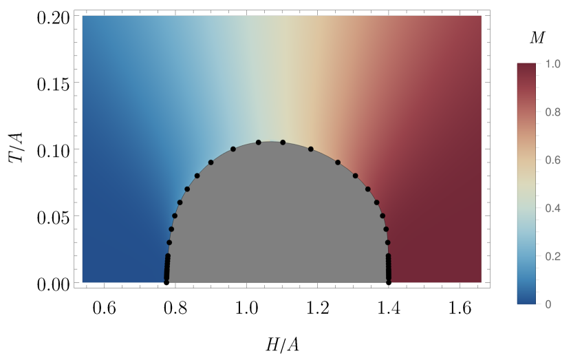
Figure 6: Magnetization of a dimerized spin system in dimension $D=3$ as function of magnetic field $H$ and temperature $T$ for inter-dimer exchange couplings $J_{T,\bm{k}=0}^{\bot}=J_{T,\bm{k}=0}^{\parallel}=J_{0}=0.2\,A$, obtained from the numerical solution of the flow equation (43). The black dots are the positions of the extrema of the susceptibility derivative $\partial^{2}M/\partial H^{2}$; see Fig. 7 (a). The black line interpolates between these points. The gray dome enclosed by this line corresponds to the antiferromagnetic $XY$ phase. There, our flow equation (43) is no longer valid because we do not consider a finite $XY$ order parameter.

One clearly sees the quantum paramagnetic phase at small and the ferromagnetic phase at large magnetic fields, as well as the thermally disordered phase at elevated temperatures. At intermediate fields and low temperatures, there is additionally the $XY$-ordered dome, where the flow equation (43) is no longer applicable. Numerically, the boundary of this dome is determined from the critical softening of the lowest ($+$) triplet mode and the associated peak in the susceptibility derivative $\partial^{2}M/\partial H^{2}$, as shown in Fig. 7 (a).

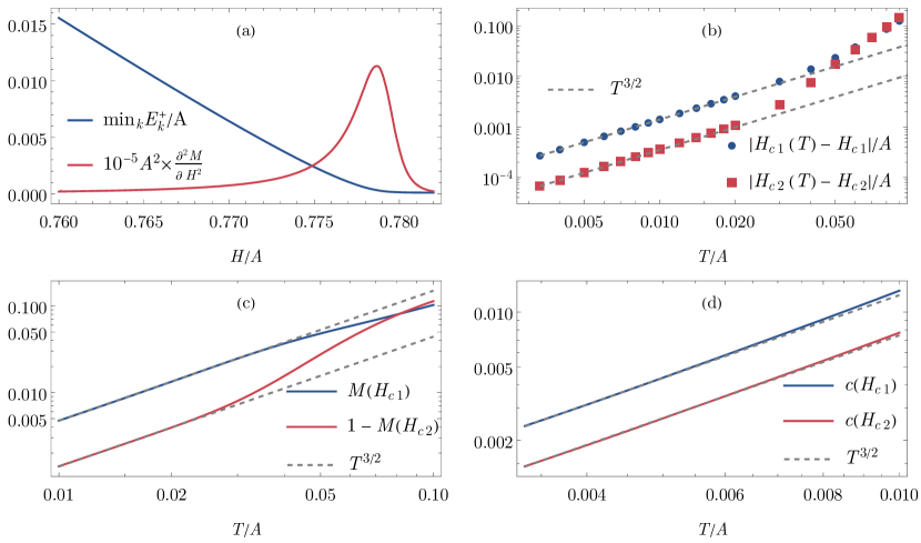
Figure 7: (a) Gap ${\rm min}_{\bm{k}}E_{\bm{k}}^{+}$ of the lowest triplet mode and susceptibility derivative $\partial^{2}M/\partial H^{2}$ as function of the magnetic field $H$ at temperature $T=0.02\,A$. We also show log-log plots of the temperature dependence of (b) the critical fields, (c) the magnetization at the quantum critical fields, and (d) the specific heat at the quantum critical fields, with the expected $T^{3/2}$ power laws for comparison. All plots are obtained from the numerical solution of the flow equations (42) and (43), for inter-dimer exchange couplings $J_{T,\bm{k}=0}^{\bot}=J_{T,\bm{k}=0}^{\parallel}=J_{0}=0.2\,A$.

With the explicit numerical solution of the flow equations (42) and (43) for the free energy and the magnetization, we can furthermore verify the various thermodynamic critical exponents that are expected for BEC quantum critical points in three dimensions. At low enough temperatures the relevant power laws are [3]

$$\left|H_{ci}(T)-H_{ci}\right|\propto{} T^{3/2},\;\;\;i=1,2,$$ (44a)

$$M(H_{c1})\propto{} T^{3/2},$$ (44b)

$$1-M(H_{c2})\propto{} T^{3/2},$$ (44c)

$$c(H_{ci})\propto{} T^{3/2},\;\;\;i=1,2,$$ (44d)

where $H_{ci}(T)$ denotes the critical fields as function of temperature, and $c(H)=-T\partial^{2}f/\partial T^{2}$ is the specific heat of the dimerized spin system. Our results for these quantities are displayed in Figs. 7 (b) – (d) on a $\log$-$\log$ scale, showing good agreement with the power laws (44). It is furthermore apparent that these asymptotic power laws can only be observed in a small temperature window [9]. For example, for the critical field shown in Fig. 7 (b) the power law is obeyed up to $T\approx 0.02\,A=0.1J_{0}$. Attempting to fit the critical field with a power law in a larger temperature window yields too large exponents in the range $1.7$ – $2.1$, in agreement with previous theoretical predictions and experimental observations [4, 6, 7, 9, 20, 3]. Ultimately, this can be traced back to the fact that the long-wavelength limit of the triplet dispersions breaks down rather quickly away from the quantum critical point because of the relative smallness of the inter-dimer exchange compared to the intra-dimer exchange [7, 9, 20].

In dimensions $D<3$, a qualitatively similar phase diagram can be obtained from the solution of the flow equation (43) for the magnetization. Unlike in $D=3$ however, the gap of the lowest triplet mode no longer closes in reduced dimensions at finite temperatures. This reflects the increased relevance of quantum fluctuations, which require a more sophisticated truncation of the spin FRG flow equations that also takes triplet-triplet interactions into account. We leave this problem for future work. However, even in this case an estimate for the critical field of the Berezinskii-Kosterlitz-Thouless or Luttinger liquid phase transition in $D=1$ or $2$ can be obtained from the peak in the susceptibility derivative, beyond which the magnetization flows to unphysical values.

III.4 Quantum fluctuations

At larger values of the inter-dimer exchange couplings and low temperatures, quantum fluctuations can also become important in the quantum paramagnetic phase. In particular, quantum fluctuations renormalize the lower critical field $H_{c1}$ given in Eq. (33) [9]. To investigate this effect, we need only consider the spin FRG flow equations for the staggered $2$-point vertex functions at zero temperature, which are given by

$$\partial_{\Lambda}\Gamma_{\Lambda,TT}^{+-}(-K,K)$$

$$={} \int_{Q}\Gamma_{\Lambda,TTTT}^{++--}(-K,-Q,Q,K)\dot{G}_{\Lambda,T}^{\bot}(Q)$$

$$+\frac{1}{2}\int_{Q}\Gamma_{\Lambda,TTTT}^{+-zz}(-K,K,-Q,Q)\dot{G}_{\Lambda,T}^{\parallel}(Q),$$ (45a)

$$\partial_{\Lambda}\Gamma_{\Lambda,TT}^{zz}(-K,K)$$

$$={} \int_{Q}\Gamma_{\Lambda,TTTT}^{+-zz}(-Q,Q,-K,K)\dot{G}_{\Lambda,T}^{\bot}(Q)$$

$$+\frac{1}{2}\int_{Q}\Gamma_{\Lambda,TTTT}^{zzzz}(-Q,Q,-K,K)\dot{G}_{\Lambda,T}^{\parallel}(Q),$$ (45b)

and shown graphically in Fig. 8.

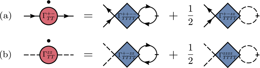
Figure 8: Diagrammatic representation of the flow equations (45) for the staggered $2$-point vertices. The meaning of the graphical elements is the same as in Figs. 3 and 5.

Since we aim to describe the quantum paramagnetic phase at $T=0$, the magnetization vanishes for all values of the deformation parameter $\Lambda$, $M_{\Lambda}=0$, so that there are no tadpole corrections to the vertex functions. Neglecting higher-order loop corrections as in Sec. III.3, we may approximate the $4$-point vertices in the above flow equations (45) by their initial values which reflect the non-trivial quantum dynamics of the staggered spin of an isolated dimer. As shown in Appendix A, for the frequency-arguments needed in the flow equations (45), the initial values of the three different $4$-point vertices associated with the staggered spin are

$$\Gamma_{0,TTTT}^{++--}(-i\omega,-i\nu,i\nu,i\omega)={} \frac{1}{A^{3}}\left[A^{2}+(H-i\omega)(H-i\nu)\right]$$

$$\times\left[A^{2}-\left(H-\frac{i\omega+i\nu}{2}\right)^{2}\right],$$ (46a)

$$\Gamma_{0,TTTT}^{+-zz}(-i\omega,i\omega,-i\nu,i\nu)={} \frac{1}{2A^{3}}\left[A^{4}-(H-i\omega)^{2}(i\nu)^{2}\right],$$ (46b)

$$\Gamma_{0,TTTT}^{zzzz}(-i\omega,i\omega,-i\nu,i\nu)={} \frac{1}{2A^{3}}\left[3A^{4}-(i\omega)^{2}(i\nu)^{2}\right.$$

$$\phantom{\frac{1}{2A^{3}}}\left.-A^{2}(i\omega)^{2}-A^{2}(i\nu)^{2}\right].$$ (46c)

Then it turns out that the staggered $2$-point vertex functions can be parametrized as

$$\Gamma_{\Lambda,TT}^{+-}(-K,K)={} \frac{A}{2}\left(1+\sigma_{\Lambda}^{\bot}\right)-A\left(\frac{H-i\omega}{AZ_{\Lambda}^{\bot}}\right)^{2}+J_{T,\bm{k}}^{\bot},$$ (47a)

$$\Gamma_{\Lambda,TT}^{zz}(-K,K)={} \frac{A}{2}\left(1+\sigma_{\Lambda}^{\parallel}\right)-A\left(\frac{i\omega}{AZ_{\Lambda}^{\parallel}}\right)^{2}+J_{T,\bm{k}}^{\parallel},$$ (47b)

where $\sigma_{\Lambda}^{\alpha}$ and $Z_{\Lambda}^{\alpha}$ are flowing renormalizations of exchange and quasiparticle residue respectively, with initial conditions $\sigma_{0}^{\alpha}=0$ and $Z_{0}^{\alpha}=1$. The transverse and longitudinal components of these couplings satisfy the flow equations

$$\partial_{\Lambda}\sigma^{\bot}_{\Lambda} =\left(Z_{\Lambda}^{\bot}\right)^{2}\int_{\bm{k}}\dot{J}^{\bot}_{\Lambda,T,\bm{k}}\frac{\partial}{\partial J^{\bot}_{\Lambda,T,\bm{k}}}\frac{4A^{2}-\epsilon_{\Lambda}^{2}(J^{\bot}_{\Lambda,T,\bm{k}})}{2A\epsilon_{\Lambda}(J^{\bot}_{\Lambda,T,\bm{k}})}+\left(Z_{\Lambda}^{\parallel}\right)^{2}\int_{\bm{k}}\dot{J}^{\parallel}_{\Lambda,T,\bm{k}}\frac{\partial}{\partial J^{\parallel}_{\Lambda,T,\bm{k}}}\frac{A}{2\epsilon_{\Lambda}(J^{\parallel}_{\Lambda,T,\bm{k}})},$$ (48a)

$$\frac{\partial_{\Lambda}Z^{\bot}_{\Lambda}}{\left(Z_{\Lambda}^{\bot}\right)^{3}} =-\left(Z_{\Lambda}^{\bot}\right)^{2}\int_{\bm{k}}\dot{J}^{\bot}_{\Lambda,T,\bm{k}}\frac{\partial}{\partial J^{\bot}_{\Lambda,T,\bm{k}}}\frac{A^{2}+2\epsilon_{\Lambda}^{2}(J^{\bot}_{\Lambda,T,\bm{k}})}{4A\epsilon_{\Lambda}(J^{\bot}_{\Lambda,T,\bm{k}})}-\left(Z_{\Lambda}^{\parallel}\right)^{2}\int_{\bm{k}}\dot{J}^{\parallel}_{\Lambda,T,\bm{k}}\frac{\partial}{\partial J^{\parallel}_{\Lambda,T,\bm{k}}}\frac{\epsilon_{\Lambda}(J^{\parallel}_{\Lambda,T,\bm{k}})}{4A},$$ (48b)

and

$$\partial_{\Lambda}\sigma^{\parallel}_{\Lambda} =\left(Z_{\Lambda}^{\bot}\right)^{2}\int_{\bm{k}}\dot{J}^{\bot}_{\Lambda,T,\bm{k}}\frac{\partial}{\partial J^{\bot}_{\Lambda,T,\bm{k}}}\frac{A}{\epsilon_{\Lambda}(J^{\bot}_{\Lambda,T,\bm{k}})}+\left(Z_{\Lambda}^{\parallel}\right)^{2}\int_{\bm{k}}\dot{J}^{\parallel}_{\Lambda,T,\bm{k}}\frac{\partial}{\partial J^{\parallel}_{\Lambda,T,\bm{k}}}\frac{3A^{2}-\epsilon_{\Lambda}^{2}(J^{\parallel}_{\Lambda,T,\bm{k}})}{2A\epsilon_{\Lambda}(J^{\parallel}_{\Lambda,T,\bm{k}})},$$ (49a)

$$\frac{\partial_{\Lambda}Z^{\parallel}_{\Lambda}}{\left(Z_{\Lambda}^{\parallel}\right)^{3}} =-\left(Z_{\Lambda}^{\bot}\right)^{2}\int_{\bm{k}}\dot{J}^{\bot}_{\Lambda,T,\bm{k}}\frac{\partial}{\partial J^{\bot}_{\Lambda,T,\bm{k}}}\frac{\epsilon_{\Lambda}(J^{\bot}_{\Lambda,T,\bm{k}})}{2A}-\left(Z_{\Lambda}^{\parallel}\right)^{2}\int_{\bm{k}}\dot{J}^{\parallel}_{\Lambda,T,\bm{k}}\frac{\partial}{\partial J^{\parallel}_{\Lambda,T,\bm{k}}}\frac{A^{2}+\epsilon_{\Lambda}^{2}(J^{\parallel}_{\Lambda,T,\bm{k}})}{4A\epsilon_{\Lambda}(J^{\parallel}_{\Lambda,T,\bm{k}})},$$ (49b)

where

$$\epsilon^{\alpha}_{\Lambda}(J)=Z_{\Lambda}^{\alpha}\sqrt{A^{2}\left(1+\sigma_{\Lambda}^{\alpha}\right)+2AJ}$$ (50)

are the flowing dispersion relations of the triplet modes at zero temperature. These flow equations are again of the form of Eq. (19) and with the Litim regulator (III.1) reduce to ordinary differential equations. Note especially that for isotropic flowing inter-dimer exchange couplings $J_{\Lambda,T,\bm{k}}^{\bot}=J_{\Lambda,T,\bm{k}}^{\parallel}$, the respective flow equations (48) and (49) for the transverse and longitudinal renormalizations are identical. Hence, $\sigma_{\Lambda}^{\bot}=\sigma_{\Lambda}^{\parallel}=\sigma_{\Lambda}$ and $Z_{\Lambda}^{\bot}=Z_{\Lambda}^{\parallel}=Z_{\Lambda}$ in this case. The resulting renormalization of the triplet modes and the lower quantum critical field at the end of the flow are shown in Fig. 9 for inter-dimer exchange couplings $J_{T,\bm{k}=0}^{\bot}=J_{T,\bm{k}=0}^{\parallel}=J_{0}$ as function of $J_{0}$.

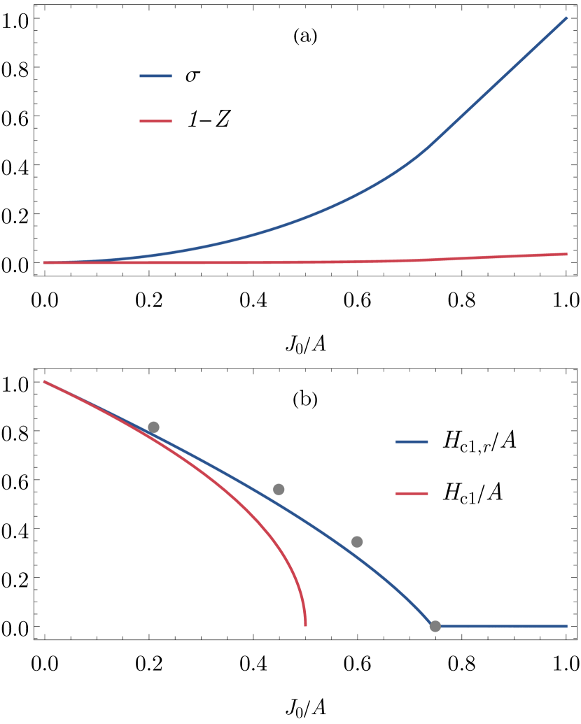
Figure 9: (a) Exchange and quasiparticle residue renormalizations of the triplet modes at $T=0$ in the quantum paramagnetic regime at the end of the flow for $\Lambda=1$, as function of the inter-dimer exchange coupling $J^{\bot}_{T,\bm{k}=0}=J^{\parallel}_{T,\bm{k}=0}=J_{0}$. (b) Renormalized lower quantum critical field $H_{c1,r}=Z_{\Lambda=1}^{\bot}\sqrt{A^{2}\left(1+\sigma_{\Lambda=1}^{\bot}\right)-2AJ^{\bot}_{T,\bm{k}=0}}$ as function of the inter-dimer exchange coupling $J^{\bot}_{T,\bm{k}=0}=J^{\parallel}_{T,\bm{k}=0}=J_{0}$, with the mean-field result $H_{c1}$ [Eq. (33)] for comparison. The gray circles are the quantum Monte Carlo results of Ref. [9].

It can be seen that for inter-dimer exchange couplings $J_{0}\gtrsim 0.2\,A$, quantum fluctuations lead to a significant renormalization of the triplet dispersions and consequently of the lower quantum critical field. On the other hand, the triplet modes remain well defined, $Z\approx 1$, even for larger inter-dimer exchange couplings. Note especially that our result for the dependence of the lower quantum critical field on the inter-dimer exchange agrees both qualitatively and quantitatively rather well with the quantum Monte Carlo simulation results of Ref. [9] at all values of the inter-dimer exchange.

IV Summary and outlook

The present work has established the applicability and power of the recently developed spin FRG formalism [23, 24, 25, 26, 27, 28] for dimerized quantum spin systems. Using a deformation scheme where the spin-correlation functions of isolated dimers define the initial conditions for the FRG flow, we have shown that even relatively simple truncations of the flow equations yield quantitatively accurate results for the spectrum and thermodynamics in the entire quantum paramagnetic, ferromagnetic, and thermally disordered phases. In particular, we have found that retaining the tadople diagrams to all orders generates a self-consistent mean-field correction to the magnetic field, which acts as a chemical potential for the triplet excitations. With this key ingredient, we have solved the flow equations for the free energy and the magnetization in a one-loop truncation. The critical softening of the lowest triplet mode has then allowed us to determine the critical magnetic field for the phase transition to the antiferromagnetic $XY$ phase at all temperatures. At low enough temperatures, our flow equations have furthermore recovered the established critical exponents that are expected for the two BEC quantum critical points. Lastly, we have demonstrated that we can also include quantum fluctuations in the quantum paramagnetic phase by deriving and solving flow equations that describe the renormalization of the triplet modes, and thereby also of the lower quantum critical field, at zero temperature.

An alternative functional renormalization group approach to quantum spin systems is based on the representation of the spin-operators in terms of Abrikosov pseudofermions [45, 46, 47, 48, 49, 50, 51] or Majorana fermions [52] and the numerical solution of the resulting truncated fermionic FRG flow equations. Apparently, so far this pseudofermion FRG approach has not been applied to dimerized spin systems. Our spin FRG suggests that this would require a proper parametrization of the quantum dynamics encoded in $4$-spin correlations of an isolated dimer, which seems to be rather difficult within the pseudofermion FRG.

Finally, let us point out that this work can be extended in several directions: On the one side, one could investigate also the antiferromagnetically ordered phase, in principle in arbitrary dimensions. On the other side, it would be interesting to study the interactions and damping of the triplet modes, in particular in the quantum critical regimes that are already accessible with the present setup of the spin FRG. Finally, it might be interesting to consider dimerized spin systems on more complicated lattices, such that quantitative comparisons with experiments come within reach.

APPENDIX A TIME-ORDERED CORRELATION FUNCTIONS OF AN ISOLATED DIMER

The isolated dimer consisting of two $S=1/2$ spins is central to our formulation of the spin FRG for dimerized quantum spin systems, because its imaginary time-ordered correlation functions define the initial condition of the FRG flow at $J_{\Lambda=0,s,ij}^{\alpha}=0$. Therefore we devote this Appendix to a short overview of the salient features of the isolated dimer, and the computation of the relevant correlation functions. The Hamiltonian of an isolated dimer reads

$$h=\frac{A}{2}\bm{S}^{2}-HS^{z};$$ (A1)

see Eq. (4b). Here, $\bm{S}=\bm{s}_{1}+\bm{s}_{2}$ denotes the total spin operator of the dimer as defined in Eq. (2), where $\bm{s}_{1}$ and $\bm{s}_{2}$ are two independent spin-$1/2$ operators. In the singlet-triplet eigenbasis of the dimer Hamiltonian (A1) that is discussed in Sec. II, the staggered and total spin operators explicitly read

$$T^{+}=\begin{pmatrix}0&0&0&1\\ -1&0&0&0\\ 0&0&0&0\\ 0&0&0&0\end{pmatrix}=(T^{-})^{\dagger},$$ (A2a)

$$T^{z}=\begin{pmatrix}0&0&1&0\\ 0&0&0&0\\ 1&0&0&0\\ 0&0&0&0\end{pmatrix},$$ (A2b)

$$S^{+}=\begin{pmatrix}0&0&0&0\\ 0&0&1&0\\ 0&0&0&1\\ 0&0&0&0\end{pmatrix}=(S^{-})^{\dagger},$$ (A2c)

$$S^{z}=\begin{pmatrix}0&0&0&0\\ 0&1&0&0\\ 0&0&0&0\\ 0&0&0&-1\end{pmatrix},$$ (A2d)

where we ordered the states in ascending order corresponding to their eigenenergies, assuming that the singlet has the lowest energy. The partition function of the isolated dimer is

$$Z=\frac{1}{p^{s}}=1+e^{-\beta E^{+}}+e^{-\beta E^{0}}+e^{-\beta E^{-}},$$ (A3)

where the eigenenergies are given in Eq. (9). From the corresponding free energy,

$$f_{0}=-\frac{1}{\beta}\ln Z,$$ (A4)

we obtain the magnetization,

$$M_{0}=-\frac{\partial f_{0}}{\partial H}=p^{+}-p^{-},$$ (A5)

and the static longitudinal susceptibility,

$$\chi_{0}=\frac{\partial M_{0}}{\partial H}=\beta\left(p^{+}+p^{-}-M_{0}^{2}\right).$$ (A6)

The Boltzmann weights are given in Eq. (10). To gain some intuitive understanding of the behavior of the isolated dimer, we plot in Fig. 10 the magnetization (A5) and static susceptibility (A6) as functions of the applied magnetic field for various temperatures.

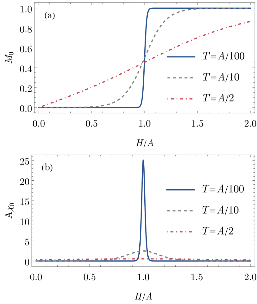
Figure 10: (a) Magnetization (A5) and (b) susceptibility (A6) of the isolated dimer, as function of applied magnetic field for different temperatures.

Because of the time reversal symmetry of the dimer Hamiltonian (A1), we can focus on $H>0$ without loss of generality. At zero temperature and for magnetic fields $H$ smaller than the intra-dimer exchange $A$, the dimer is in the singlet state, $p^{s}=1$. Precisely at $H=A$, the dimer undergoes a field induced quantum phase transition into the fully polarized $+$ triplet state with $p^{+}=1$. Thus, at zero temperature the magnetization is a simple step function, $M_{0}(T=0)=\Theta(H-A)$. At finite temperatures, on the other hand, all dimer states are thermally occupied according to their respective Boltzmann factors (10), implying a smooth magnetization curve. Saturation is no longer reached once the temperature is sufficient to excite non-magnetic states. Further increasing the temperature results in the magnetization becoming more linear, with a slope proportional to the inverse temperature. Correspondingly, the susceptibility exhibits a single $\delta$-like peak at the critical field $H=A$, which widens and becomes field independent in leading order towards high temperatures.

For the initial conditions of the vertex expansion, we require the imaginary-time ordered connected $n$-point correlation function of the staggered and total dimer spin as well. They are defined as

$$\delta(\omega_{1}+\ldots+\omega_{n})G_{0,\underbrace{\scriptstyle S\ldots S}_{m}\underbrace{\scriptstyle T\ldots T}_{n-m}}^{\alpha_{1}\ldots\alpha_{n}}(i\omega_{1},\ldots,i\omega_{n})={} \int_{0}^{\beta}d\tau_{1}\ldots\int_{0}^{\beta}d\tau_{n}e^{i(\omega_{1}\tau_{1}+\ldots+\omega_{n}\tau_{n})}$$

$$\times\braket{{\cal T}S^{\alpha_{1}}(\tau_{1})\ldots S^{\alpha_{m}}(\tau_{m})T^{\alpha_{m+1}}(\tau_{m+1})\ldots T^{\alpha_{n}}(\tau_{n})}_{\rm connected}.$$ (A7)

Here, ${\cal{T}}$ denotes time-ordering in imaginary time, and the imaginary time dependence of the operators is in the Heisenberg picture. We also used the energy conservation to factor out the frequency-$\delta$, which is defined as $\delta(\omega)=\beta\delta_{\omega,0}$. In frequency space, the connected spin correlation functions (A) can be calculated efficiently using their spectral representations. Since the eigenenergies (9) of the Hamiltonian (A1) as well as the matrix representations (A2) of the spin operators are known, one can carry out the required Fourier transformation explicitly [37]. The $2$-point functions are given by

$$G_{0,TT}^{+-}(i\omega,-i\omega) =G_{0,T}^{\bot}(i\omega)=\sum_{r=\pm}\frac{p^{s}-p^{r}}{A-r\left(H-i\omega\right)},$$ (A8a)

$$G_{0,TT}^{zz}(i\omega,-i\omega) =G_{0,T}^{\parallel}(i\omega)=\frac{2A\left(p^{s}-p^{0}\right)}{A^{2}+\omega^{2}},$$ (A8b)

$$G_{0,SS}^{+-}(i\omega,-i\omega) =G_{0,S}^{\bot}(i\omega)=\frac{M_{0}}{H-i\omega},$$ (A8c)

$$G_{0,SS}^{zz}(i\omega,-i\omega) =G_{0,S}^{\parallel}(i\omega)=\delta_{\omega,0}\chi_{0}.$$ (A8d)

Note that the longitudinal total spin has no dynamics, $G_{0,S}^{\parallel}(i\omega)\propto\delta_{\omega,0}$, reflecting the $U(1)$ spin-rotational symmetry of the dimer Hamiltonian (A1) around the direction of the magnetic field. The finite longitudinal and mixed transverse-longitudinal $3$-point functions are

$$G_{0,TTS}^{zzz}(i\omega_{1},i\omega_{2},i\omega_{3})={} -\delta(\omega_{3})M_{0}G_{0,T}^{\parallel}(i\omega_{3}),$$ (A9a)

$$G_{0,SSS}^{zzz}(i\omega_{1},i\omega_{2},i\omega_{3})={} \delta(\omega_{2})\delta(\omega_{3})M_{0}\left(1-3\beta^{-1}\chi_{0}-M_{0}^{2}\right)=\delta_{\omega_{2},0}\delta_{\omega_{3},0}\partial_{H}\chi_{0},$$ (A9b)

and

$$G_{0,TTS}^{+-z}(i\omega_{1},i\omega_{2},i\omega_{3})={} \frac{G_{0,T}^{\bot}(i\omega_{1})-G_{0,T}^{\bot}(-i\omega_{2})}{i\omega_{3}}-\delta(\omega_{3})\left[\sum_{r=\pm}\frac{rp^{r}}{A-r\left(H-i\omega_{1}\right)}+M_{0}G_{0,T}^{\bot}(i\omega_{1})\right],$$ (A10a)

$$G_{0,TST}^{+-z}(i\omega_{1},i\omega_{2},i\omega_{3})={} \frac{G_{0,S}^{\bot}(i\omega_{1})}{M_{0}}\left[G_{0,T}^{\parallel}(i\omega_{3})-G_{0,T}^{\bot}(i\omega_{1})\right],$$ (A10b)

$$G_{0,STT}^{+-z}(i\omega_{1},i\omega_{2},i\omega_{3})={} \frac{G_{0,S}^{\bot}(i\omega_{1})}{M_{0}}\left[G_{0,T}^{\parallel}(i\omega_{3})-G_{0,T}^{\bot}(-i\omega_{2})\right],$$ (A10c)

$$G_{0,SSS}^{+-z}(i\omega_{1},i\omega_{2},i\omega_{3})={} \frac{G_{0,S}^{\bot}(i\omega_{1})}{M_{0}}\left[-G_{0,S}^{\bot}(-i\omega_{2})+M_{0}G_{0,S}^{\parallel}(i\omega_{3})\right].$$ (A10d)

For the calculation of the quantum fluctuations in Sec. III.4, we also require the initial conditions of the staggered $4$-point vertices, which are determined by the staggered $4$-point correlation functions of the isolated dimer via the tree expansion; see Eq. (B24) and Refs. [41, 23, 26]. After some tedious calculations we find that the different components of the staggered $4$-spin correlation functions of an isolated dimer are given by the following expressions,

$$G_{0,TTTT}^{++--}(i\omega_{1},\ldots,i\omega_{4})$$

$$={} \frac{\left[2\left(A+H\right)+i\omega_{3}+i\omega_{4}\right]\left[2\left(A-H\right)-i\omega_{3}-i\omega_{4}\right]}{2H+i\omega_{3}+i\omega_{4}}$$

$$\times\sum_{r=\pm}\frac{r\left(p^{r}-p^{s}\right)}{\left[A-r\left(H-i\omega_{1}\right)\right]\left[A-r\left(H-i\omega_{2}\right)\right]\left[A-r\left(H+i\omega_{3}\right)\right]\left[A-r\left(H+i\omega_{4}\right)\right]}$$

$$+\left[\delta\left(\omega_{1}+\omega_{3}\right)+\delta\left(\omega_{1}+\omega_{4}\right)\right]$$

$$\times\left\{\sum_{r=\pm}\frac{p^{r}}{\left[A-r\left(H-i\omega_{1}\right)\right]\left[A-r\left(H-i\omega_{2}\right)\right]}+\frac{4A^{2}p^{s}}{\left[A^{2}-\left(H-i\omega_{1}\right)^{2}\right]\left[A^{2}-\left(H-i\omega_{2}\right)^{2}\right]}-G_{0,T}^{\bot}(i\omega_{1})G_{0,T}^{\bot}(i\omega_{2})\right\},$$ (A11a)

$$G_{0,TTTT}^{+-zz}(i\omega_{1},\ldots,i\omega_{4})$$

$$={} \sum_{r=\pm}\frac{rp^{r}}{\left[A-r\left(H-i\omega_{1}\right)\right]\left[A-r\left(H+i\omega_{2}\right)\right]}\left(\frac{1}{H+i\omega_{2}+i\omega_{3}}+\frac{1}{H+i\omega_{2}+i\omega_{4}}\right)$$

$$-p^{s}\sum_{r=\pm}\left\{\frac{1}{\left[A+r\left(H-i\omega_{1}\right)\right]\left(A-ri\omega_{3}\right)}\left(\frac{1}{A+r\left(H+i\omega_{2}\right)}+\frac{1}{A+ri\omega_{4}}\right)+\left(i\omega_{3}\leftrightarrow i\omega_{4}\right)\right\}$$

$$-\frac{2Ap^{0}\left(i\omega_{3}-i\omega_{4}\right)^{2}}{\left(H+i\omega_{2}+i\omega_{3}\right)\left(H+i\omega_{2}+i\omega_{4}\right)\left(A^{2}+\omega_{3}^{2}\right)\left(A^{2}+\omega_{4}^{2}\right)}$$

$$+\delta\left(\omega_{1}+\omega_{2}\right)\left\{\frac{4A^{2}p^{s}}{\left[A^{2}-\left(H-i\omega_{1}\right)^{2}\right]\left(A^{2}+\omega_{3}^{2}\right)}-G_{0,T}^{\bot}(i\omega_{1})G_{0,T}^{\parallel}(i\omega_{3})\right\},$$ (A11b)

$$G_{0,TTTT}^{zzzz}(i\omega_{1},\ldots,i\omega_{4})$$

$$={} \frac{4A^{2}\left(p^{0}-p^{s}\right)\left[6A^{4}-2\omega_{1}\omega_{2}\omega_{3}\omega_{4}+A^{2}\left(\omega_{1}^{2}+\omega_{2}^{2}+\omega_{3}^{2}+\omega_{4}^{2}\right)\right]}{\left(A^{2}+\omega_{1}^{2}\right)\left(A^{2}+\omega_{2}^{2}\right)\left(A^{2}+\omega_{3}^{2}\right)\left(A^{2}+\omega_{4}^{2}\right)}$$

$$+\left\{\delta\left(\omega_{1}+\omega_{2}\right)\left[\frac{4A^{2}\left(p^{0}+p^{s}\right)}{\left(A^{2}+\omega_{1}^{2}\right)\left(A^{2}+\omega_{3}^{2}\right)}-G_{0,T}^{\parallel}(i\omega_{1})G_{0,T}^{\parallel}(i\omega_{3})\right]+\left(i\omega_{2}\leftrightarrow i\omega_{3}\right)+\left(i\omega_{2}\leftrightarrow i\omega_{4}\right)\right\}.$$ (A11c)

APPENDIX B DETAILS OF THE SPIN FRG FORMALISM

In order to set up the spin FRG for our dimerized spin system (1), it is convenient to introduce the following compact notation: We collect all field labels into a collective label $x\equiv(\alpha ai\tau)$, where $\alpha=x,y,z$ labels the Cartesian component, $a=S,T$ the field flavor, $i=1,\ldots,N$ the dimer, and $\tau$ is the imaginary time. We then define the collection $I_{x}$ of total and staggered spin operators such that

$$\left(\begin{matrix}I_{S,i}^{x}(\tau)\\ I_{S,i}^{y}(\tau)\\ I_{S,i}^{z}(\tau)\\ I_{T,i}^{x}(\tau)\\ I_{T,i}^{y}(\tau)\\ I_{T,i}^{z}(\tau)\end{matrix}\right)=\left(\begin{matrix}S_{i}^{x}(\tau)\\ S_{i}^{y}(\tau)\\ S_{i}^{z}(\tau)\\ T_{i}^{x}(\tau)\\ T_{i}^{y}(\tau)\\ T_{i}^{z}(\tau)\end{matrix}\right).$$ (B12)

In the space of this collective label, the (deformed) inter-dimer exchange matrix is given by

$$\left({\bf J}_{\Lambda}\right)_{xx^{\prime}}={} \delta^{\alpha\alpha^{\prime}}\delta_{aa^{\prime}}\delta(\tau-\tau^{\prime})$$

$$\times\left[\left(1-\delta^{\alpha z}\right)J_{\Lambda,a,ii^{\prime}}^{\bot}+\delta^{\alpha z}J_{\Lambda,a,ii^{\prime}}^{\parallel}\right].$$ (B13)

With this compact notation, the generating functional of connected spin correlation functions can be written as

$${\cal G}_{\Lambda}[h]=\ln{\rm Tr}\left[e^{-\beta{\cal H}_{0}}{\cal T}e^{\int_{x}h_{x}I_{x}-\frac{1}{2}\int_{xx^{\prime}}I_{x}\left({\bf J}_{\Lambda}\right)_{xx^{\prime}}I_{x^{\prime}}}\right],$$ (B14)

where $h_{x}$ is the source field conjugate to the operator $I_{x}$, the integration symbol is $\int_{x}=\sum_{\alpha}\sum_{a}\sum_{i}\int_{0}^{\beta}d\tau$, and ${\cal T}$ denotes imaginary-time ordering of everything to its right. All spin operators $I_{x}$ are taken to be in the imaginary-time Heisenberg picture with respect to the Hamiltonian ${\cal H}_{0}$ of decoupled dimers given in Eq. (4). Ideally, we would like to work exclusively with one-line irreducible vertices [41, 23]. Their generating functional is the Legendre transformation of the generating functional (B14) of connected correlation functions. However, because the dimer Hamiltonian (4) possesses $U(1)$ spin-rotational symmetry around the $z$ axis, such a Legendre transformation is not well-defined when we turn off the inter-dimer exchange ${\bf J}_{\Lambda}$ at the initial scale of the RG flow [25]. Ultimately, the reason for this is that $S_{i}^{z}$ is conserved for each dimer and hence has no dynamics [see Eq. (A8d)], which makes it impossible to express the conjugate source via the respective average field. To circumvent this issue, it is convenient [25] to work with a hybrid functional

$${\cal F}_{\Lambda}[h]={\cal G}_{\Lambda}\left[({\bf 1}-{\bf P})h-{\bf P}{\bf J}_{\Lambda}h\right]-\frac{1}{2}\int_{xx^{\prime}}h_{x}\left({\bf P}{\bf J}_{\Lambda}\right)_{xx^{\prime}}h_{x^{\prime}},$$ (B15)

where the matrix ${\bf P}={\bf P}^{2}$ with components

$$\left({\bf P}\right)_{xx^{\prime}}=\delta^{\alpha\alpha^{\prime}}\delta_{aa^{\prime}}\delta_{ii^{\prime}}\delta(\tau-\tau^{\prime})\delta^{\alpha z}\delta_{aS}$$ (B16)

projects onto the longitudinal magnetization subspace. The functional (B15) generates connected correlation functions of the staggered and the transverse dimer spin and amputated connected longitudinal dimer spin correlation functions. The associated generating functional of one-line irreducible vertices is then well-defined at the initial scale; it is explicitly given by

$$\Gamma_{\Lambda}[\varphi]={} \int_{x}h_{x}\left(\phi_{\Lambda,x}+\varphi_{x}\right)-{\cal F}_{\Lambda}[h]$$

$$-\frac{1}{2}\int_{xx^{\prime}}\varphi_{x}\left({\bf R}_{\Lambda}\right)_{xx^{\prime}}\varphi_{x^{\prime}},$$ (B17)

where

$${\bf R}_{\Lambda}=\left({\bf 1}-{\bf P}\right)\left({\bf J}_{\Lambda}-{\bf J}\right)\left({\bf 1}-{\bf P}\right)+{\bf P}\left(-{\bf J}_{\Lambda}^{-1}+{\bf J}^{-1}\right){\bf P}$$ (B18)

is the regulator matrix, and the source fields $h_{x}[\varphi]$ are determined by inversion of

$$\frac{\delta{\cal F}_{\Lambda}[h]}{\delta h_{x}}=\phi_{\Lambda,x}+\varphi_{x},$$ (B19)

with the vacuum expectation values

$$\left.\frac{\delta{\cal F}_{\Lambda}[h]}{\delta h_{x}}\right|_{h=0}=\phi_{\Lambda,x}.$$ (B20)

Note that compared to Refs. [23, 25, 26], we use a slightly different regulator subtraction with the fluctuating fields $\varphi_{x}$ instead of the full field $\phi_{\Lambda,x}+\varphi_{x}$ in the second line of the generating functional (B17). This turns out to be more convenient in the presence of finite vacuum expectation values $\phi_{\Lambda,x}$, because $\phi_{\Lambda,x}$ can then be chosen as the flowing field configuration that minimizes $\Gamma_{\Lambda}[\varphi]$ for vanishing source fields $h_{x}$; i.e.,

$$\left.\frac{\delta\Gamma_{\Lambda}[\varphi]}{\delta\varphi_{x}}\right|_{\varphi=0}=0.$$ (B21)

By taking derivatives with respect to the deformation parameter $\Lambda$, it can be shown that the generating functionals ${\cal G}_{\Lambda}[h]$, ${\cal F}_{\Lambda}[h]$, and $\Gamma_{\Lambda}[\varphi]$ given in Eqs. (B14), (B15) and (B17) respectively satisfy exact flow equations which determine the evolution of the associated correlation functions when the exchange interaction is gradually deformed. Because the spin operators at different lattice sites commute, these equations are formally identical to the FRG flow equations for bosons. For an explicit derivation of these flow equations, we refer to Refs. [23, 25]. Here, we only require the flow equation of the generating functional (B17) of irreducible vertex functions. It has the form of a bosonic Wetterich equation [38],

$$\partial_{\Lambda}\Gamma_{\Lambda}[\varphi]-\int_{x}\frac{\delta\Gamma_{\Lambda}[\varphi]}{\delta\varphi_{x}}\partial_{\Lambda}\phi_{\Lambda,x}$$

$$={} \frac{1}{2}{\rm Tr}\left\{\left(\partial_{\Lambda}{\bf R}_{\Lambda}\right)\left[\left({\bf\Gamma}^{\prime\prime}_{\Lambda}[\varphi]+{\bf R}_{\Lambda}\right)^{-1}+{\bf P}{\bf J}_{\Lambda}{\bf P}\right]\right\}$$

$$+\frac{1}{2}\int_{xx^{\prime}}\phi_{\Lambda,x}\left(\partial_{\Lambda}{\bf R}_{\Lambda}\right)_{xx^{\prime}}\phi_{\Lambda,x^{\prime}}$$

$$+\int_{xx^{\prime}}\varphi_{x}\partial_{\Lambda}\left[\left({\bf R}_{\Lambda}\right)_{xx^{\prime}}\phi_{\Lambda,x^{\prime}}\right],$$ (B22)

where

$$\left({\bf\Gamma}^{\prime\prime}_{\Lambda}[\varphi]\right)_{xx^{\prime}}=\frac{\delta^{2}\Gamma_{\Lambda}[\varphi]}{\delta\varphi_{x}\delta\varphi_{x^{\prime}}}$$ (B23)

denotes the matrix of second functional derivatives of the generating functional, and the trace runs over the collective label $x$.

In the last step, we have to specify the initial condition for the generating functional $\Gamma_{\Lambda}[\varphi]$. In a vertex expansion scheme, this initial condition can be obtained from the correlation functions of isolated dimers given in Appendix A via the tree expansion [41, 23, 26]. This amounts to expanding both sides of

$$\frac{\delta^{2}{\cal F}_{\Lambda}[h]}{\delta h_{x}\delta h_{x^{\prime}}}=\left({\bf\Gamma}^{\prime\prime}_{\Lambda}[\varphi]+{\bf R}_{\Lambda}\right)^{-1}_{xx^{\prime}}$$ (B24)

in powers of the source fields $h_{x}$ and comparing coefficients at $\Lambda=0$.

References

- [1] Ch. Rüegg, N. Cavadini, A. Furrer, H.-U. Güdel, K. Krämer, H. Mutka, A. Wildes, K. Habicht, and P. Vorderwisch, Bose–Einstein condensation of the triplet states in the magnetic insulator , Nature 423, 62 (2003).
- [2] T. Giamarchi, C. Rüegg, and O. Tchernyshyov, Bose–Einstein condensation in magnetic insulators, Nature Phys. 4, 198 (2008).
- [3] V. Zapf, M. Jaime, and C. D. Batista, Bose-Einstein condensation in quantum magnets, Rev. Mod. Phys. 86, 563 (2014).
- [4] T. Nikuni, M. Oshikawa, A. Oosawa, and H. Tanaka, Bose-Einstein Condensation of Dilute Magnons in , Phys. Rev. Lett. 84, 5868 (2000).
- [5] N. Cavadini, Ch. Rüegg, W Henggeler, A. Furrer, H.-U. Güdel, K. Krämer, and H. Mutka, Temperature renormalization of the magnetic excitations in , Eur. Phys. J. B 18, 565 (2000).
- [6] A. Oosawa, H. Aruga Katori, and H. Tanaka, Specific heat study of the field-induced magnetic ordering in the spin-gap system , Phys. Rev. B 63, 134416 (2001).
- [7] E. Ya. Sherman, P. Lemmens, B. Busse, A. Oosawa, and H. Tanaka, Sound Attenuation Study on the Bose-Einstein Condensation of Magnons in , Phys. Rev. Lett. 91, 057201 (2003).
- [8] M. Matsumoto, B. Normand, T. M. Rice, and M. Sigrist, Field- and pressure-induced magnetic quantum phase transitions in , Phys. Rev. B 69, 054423 (2004).
- [9] O. Nohadani, S. Wessel, B. Normand, and S. Haas, Universal scaling at field-induced magnetic phase transitions, Phys. Rev. B 69, 220402(R) (2004).
- [10] Ch. Rüegg, B. Normand, M. Matsumoto, Ch. Niedermayer, A. Furrer, K. W. Krämer, H.-U. Güdel, Ph. Bourges, Y. Sidis, and H. Mutka, Quantum Statistics of Interacting Dimer Spin Systems, Phys. Rev. Lett. 95, 267201 (2005).
- [11] M. Jaime, V. F. Correa, N. Harrison, C. D. Batista, N. Kawashima, Y. Kazuma, G. A. Jorge, R. Stern, I. Heinmaa, S. A. Zvyagin, Y. Sasago, and K. Uchinokura, Magnetic-Field-Induced Condensation of Triplons in Han Purple Pigment , Phys. Rev. Lett. 93, 087203 (2004).
- [12] S. E. Sebastian, N. Harrison, C. D. Batista, L. Balicas, M. Jaime, P. A. Sharma, N. Kawashima, and I. R. Fisher, Dimensional reduction at a quantum critical point, Nature 441, 617 (2006).
- [13] C. D. Batista, J. Schmalian, N. Kawashima, P. Sengupta, S. E. Sebastian, N. Harrison, M. Jaime, and I. R. Fisher, Geometric Frustration and Dimensional Reduction at a Quantum Critical Point, Phys. Rev. Lett. 98, 257201 (2007).
- [14] Ch. Rüegg, D. F. McMorrow, B. Normand, H. M. Rønnow, S. E. Sebastian, I. R. Fisher, C. D. Batista, S. N. Gvasaliya, Ch. Niedermayer, and J. Stahn, Multiple Magnon Modes and Consequences for the Bose-Einstein Condensed Phase in , Phys. Rev. Lett. 98, 017202 (2007).
- [15] X.-G. Zhou, Yuan Yao, Y. H. Matsuda, A. Ikeda, A. Matsuo, K. Kindo, and H. Tanaka, Particle-Hole Symmetry Breaking in a Spin-Dimer System Observed at T, Phys. Rev. Lett. 125, 267207 (2020).
- [16] M. Matsumoto, B. Normand, T. M. Rice, and M. Sigrist, Magnon Dispersion in the Field-Induced Magnetically Ordered Phase of , Phys. Rev. Lett. 89, 077203 (2002).
- [17] N. Cavadini, W. Henggeler, A. Furrer, H.-U. Güdel, K. Krämer and H. Mutka, Magnetic excitations in the quantum spin system , Eur. Phys. J. B 7, 519 (1999).
- [18] N. Cavadini, G. Heigold, W. Henggeler, A. Furrer, H.-U. Güdel, K. Krämer, and H. Mutka, Magnetic excitations in the quantum spin system , Phys. Rev. B 63, 172414 (2001).
- [19] N. Cavadini, Ch. Rüegg, A. Furrer, H.-U. Güdel, K. Krämer, H. Mutka, and P. Vorderwisch, Triplet excitations in low- spin-gap systems and : An inelastic neutron scattering study, Phys. Rev. B 65, 132415 (2002).
- [20] J. Sirker, A. Weiße, and O. P. Sushkov, The Field-Induced Magnetic Ordering Transition in , J. Phys. Soc. Jpn. 74, 129 (2005).
- [21] Y. Sasago, K. Uchinokura, A. Zheludev, and G. Shirane, Temperature-dependent spin gap and singlet ground state in , Phys. Rev. B 55, 8357 (1997).
- [22] M. Tachiki and T. Yamada, Spin Ordering in a Spin-Pair System, J. Phys. Soc. Jpn. 28, 1413 (1970).
- [23] J. Krieg and P. Kopietz, Exact renormalization group for quantum spin systems, Phys. Rev. B 99, 060403(R) (2019).
- [24] D. Tarasevych, J. Krieg, and P. Kopietz, A rich man’s derivation of scaling laws for the Kondo model, Phys. Rev. B 98, 235133 (2018).
- [25] R. Goll, D. Tarasevych, J. Krieg, and P. Kopietz, Spin functional renormalization group for quantum Heisenberg ferromagnets: Magnetization and magnon damping in two dimensions, Phys. Rev. B 100, 174424 (2019).
- [26] R. Goll, A. Rückriegel, and P. Kopietz, Zero-magnon sound in quantum Heisenberg ferromagnets, Phys. Rev. B 102, 224437 (2020).
- [27] D. Tarasevych and P. Kopietz, Dissipative spin dynamics in hot quantum paramagnets, Phys. Rev. B 104, 024423 (2021).
- [28] D. Tarasevych and P. Kopietz, Critical spin dynamics of Heisenberg ferromagnets revisited, Phys. Rev. B 105, 024403 (2022).
- [29] T. Machado and N. Dupuis, From local to critical fluctuations in lattice models: A nonperturbative renormalization-group approach, Phys. Rev. E 82, 041128 (2010).
- [30] A. Rançon and N. Dupuis, Nonperturbative renormalization group approach to the Bose-Hubbard model, Phys. Rev. B 83, 172501 (2011).
- [31] A. Rançon and N. Dupuis, Nonperturbative renormalization group approach to strongly correlated lattice bosons, Phys. Rev. B 84, 174513 (2011).
- [32] A. Rançon and N. Dupuis, Universal thermodynamics of a two-dimensional Bose gas, Phys. Rev. A 85, 063607 (2012).
- [33] A. Rançon and N. Dupuis, Thermodynamics of a Bose gas near the superfluid-Mott-insulator transition, Phys. Rev. A 86, 043624 (2012).
- [34] A. Rançon, Nonperturbative renormalization group approach to quantum XY spin models, Phys. Rev. B 89, 214418 (2014).
- [35] V. G. Vaks, A. I. Larkin, S. A. Pikin, Thermodynamics of an Ideal Ferromagnetic Substance, Zh. Eksp. Teor. Fiz. 53, 281 (1967) [ Sov. Phys. JETP 26, 188 (1968) ].
- [36] V. G. Vaks, A. I. Larkin, and S. A. Pikin, Spin waves and correlation functions in a ferromagnetic, Zh. Eksp. Teor. Fiz. 53, 1089 (1967) [ Sov. Phys. JETP 26, 647 (1968) ].
- [37] Yu. A. Izyumov and Yu. N. Skryabin, Statistical Mechanics of Magnetically Ordered Systems (Springer, Berlin, 1988).
- [38] C. Wetterich, Exact evolution equation for the effective potential, Phys. Lett. B 301, 90 (1993).
- [39] J. Berges, N. Tetradis, and C. Wetterich, Non-perturbative renormalization flow in quantum field theory and statistical physics, Phys. Rep. 363, 223 (2002).
- [40] J. M. Pawlowski, Aspects of the functional renormalisation group, Ann. Phys. 322, 2831 (2007).
- [41] P. Kopietz, L. Bartosch, and F. Schütz, Introduction to the Functional Renormalization Group, (Springer, Berlin, 2010).
- [42] W. Metzner, M. Salmhofer, C. Honerkamp, V. Meden, and K. Schönhammer, Functional renormalization group approach to correlated fermion systems, Rev. Mod. Phys. 84, 299 (2012).
- [43] N. Dupuis, L. Canet, A. Eichhorn, W. Metzner, J. M. Pawlowski, M. Tissier, and N. Wschebor, The nonperturbative functional renormalization group and its applications, Phys. Rep. 910, 1 (2021).
- [44] D. F. Litim, Optimized renormalization group flows, Phys. Rev. D 64, 105007 (2001).
- [45] J. Reuther and P. Wölfle, - frustrated two-dimensional Heisenberg model: Random phase approximation and functional renormalization group, Phys. Rev. B 81, 144410 (2010).
- [46] J. Reuther and R. Thomale, Functional renormalization group for the anisotropic triangular antiferromagnet, Phys. Rev. B 83, 024402 (2011).
- [47] J. Reuther, R. Thomale, and S. Trebst, Finite-temperature phase diagram of the Heisenberg-Kitaev model, Phys. Rev. B 84, 100406(R) (2011).
- [48] F. L. Buessen and S. Trebst, Competing magnetic orders and spin liquids in two- and three-dimensional kagome systems: Pseudofermion functional renormalization group perspective, Phys. Rev. B 94, 235138 (2016).
- [49] J. Thoenniss, M. K. Ritter, F. B. Kugler, J. von Delft, and M. Punk, Multiloop pseudofermion functional renormalization for quantum spin systems: Application to the spin- kagome Heisenberg model, arXiv:2011.01268v1 [cond-mat.str-el] 2 Nov 2020.
- [50] D. Kiese, T. Müller, Y. Iqbal, R. Thomale, and S. Trebst, Multiloop functional renormalization group approach to quantum spin systems, Phys. Rev. Research 4, 023185 (2022).
- [51] M. K. Ritter, D. Kiese, T. Müller, F. B. Kugler, R. Thomale, S. Trebst, and J. von Delft, Benchmark Calculations of Multiloop Pseudofermion fRG, arXiv: 2203.13007 [cond-mat.str-el] 24 Mar 2022.
- [52] N. Niggemann, B. Sbierski, and J. Reuther, Frustrated Quantum Spins at finite Temperature: Pseudo-Majorana functional RG approach, Phys. Rev. B 103, 104431 (2021).