The impact of thermal noise on kink propagation through a heterogeneous system

Abstract

The impact of thermal noise on kink motion through the curved region of the long Josephson junction is studied. On the basis of the Fokker-Planck equation the analytical formula that describes the probability of transmission of the kink over the potential barrier is proposed. The analytical results are compared with the simulations based on the field model.

PACS numbers: 05.45.Yv, 85.25.Cp, 74.50.+r, 05.10.Gg

1 Introduction

In recent years, a significant increase of interest in the construction of a variety of appliances that use superconducting elements is observed. Among the devices manufactured on the basis of superconductors, Josephson junctions occupy a prominent position. The effect of supercurrent flow without any voltage applied was initially predicted by Brian D. Josephson [1, 2]. A device known as a Josephson junction consists of two superconductors coupled by some weak link. The weak link can be made of a thin insulating barrier (in S-I-S junctions), normal non-superconducting metal (in S-N-S junctions), or have a form of constriction that weakens the superconductivity at the point of contact (in S-s-S junctions). The effect was experimentally confirmed by Philip Anderson and John Rowell [3].

Presently there are a variety of devices which contain Josephson junctions in their design [4, 5]. They can be classified into three groups. In the first group one can include antennas, amplifiers, filters, bolometers, single photon detectors, magnetometers and many others. The second group consists of digital electronic appliances like digital-to-analogue and analogue-to-digital converters and rapid single flux quantum computing elements. The third group consists of quantum computing devices.

In the context of future technical applications of the Josephson junction it is natural to look for superconducting materials with high critical temperatures. Presently at normal pressure, it is possible to achieve a state of superconductivity at relatively high temperatures in the so-called high-temperature superconductors [6]. An example of such materials is cuprate-perovskite ceramic which has a critical temperature above 90 K. Nowadays one of the highest - temperature superconductors is $HgBa_{2}Ca_{2}Cu_{3}O_{8+\delta}$ with a critical temperature exceeding 133 K [7]. In particular, exceeding the temperature 77 K allows the use of liquid nitrogen, on an industrial scale, in cooling systems of superconducting devices.

The Josephson junction properties required for optimal performance of the appropriate devices can be planned at the design stage of the equipment that uses them. Between multiple approaches directed at obtaining requested properties of Josephson junctions, shape engineering plays a significant role. In this approach, particular modifications of the junction shape are proposed in order to obtain their required properties. For example, in the article [8] the authors proposed a device that consists of a junction with an exponentially tapered width, decreasing toward the load. In this device the junction is preceded by an idle region, where the oxide layer is thicker, preventing the tunnelling of Cooper pairs.

On the other hand, in the heart-shaped annular junction two classical vortex states can be prepared, corresponding to two minima of the potential [9]. The bias current across the junction is used to slant the potential. The strength and direction of the the applied external magnetic field plays the role of the control parameters. For example, all these parameters can be used in order to modify the barrier height. The heart-shaped long Josephson junction placed in an in-plane external magnetic field was also considered in article [10]. Based on this geometry the authors designed a classical system with two ground states. At sufficiently low temperatures, this structure is expected to behave as a quantum two-state system.

The other opportunity to modify properties of a junction is formation of the T-shaped geometry [11]. The above mentioned appliance consists of two perpendicular Josephson T-Lines forming a T junction. The particular effect present in the device is the creation of a new vortex when an original vortex, moving along the main Josephson T-line, is passing the T junction. The new vortex created at the T junction begins its motion in the direction perpendicular to the main Josephson T-line. The creation of a new vortex is substantially dependent on the energy of the original vortex. If the kinetic energy of the original vortex is too small then the T junction acts as a barrier and the original vortex is reflected without creation of a new vortex.

A similar, to some degree, proposal is sigma-pump. The main advantage of this system is the lack of the barrier associated with the T-junction present in the T-pump. Instead, the Josephson transmission line is connected with the ring smoothly through the Y junction. In this pump a nucleation barrier is absent. Moreover, the nucleation energy is gathered by the trapped fluxon during its motion in the potential associated with increasing width. A similar system is considered in articles [12] and [13].

An interesting possibility is an annular junction delimited by two closely spaced confocal ellipses that is characterized by a periodically modulated width [14, 15]. This spatial dependence, in turn, produces a periodic potential that interchangeably attracts and repels the fluxons. In this particular junction double-well potential, experienced by an individual fluxon, is produced by an intrinsic non-uniform width.

If the thickness of the dielectric layer in the junction is position dependent then the kink experiences the effective potential originating in heterogeneities present in the system [16]. The value of transmission critical current in this case is strictly determined by the parameters of the system.

The effects of arbitrary curvature on fluxon motion in curved Josephson junctions were studied in articles [17, 18, 19, 20, 21] with curvatures playing the role of potential barriers for kink motion. In particular in [22] the different simplified effective descriptions were compared in order to choose the most suitable for the considered system.

In the present article we study the curved system with bias current and the quasi-particle dissipation taken into account. Moreover this paper is aimed at studying the effects of nonzero temperature of the system on the process of penetration of the potential barrier through the kink. We present the appropriate analytical results and compare them with the results of simulations performed in the field model. The analytical approximations rely mainly on the projection onto energy density method.

2 Kink in curved system

We consider the kink motion in the sine-Gordon model with position dependent dispersive term

$$\partial_{t}^{2}\phi+\alpha\partial_{t}\phi-\partial_{x}({\cal F}(x)\partial_{x}\phi)+\sin\phi=-\Gamma.$$ (1)

The physical motivation for description of curvature effects in the framework of this model was described in detail in the articles [22, 19]. In this paper it was shown that this modification appears in the description of a curved Josephson junction. The function ${\cal F}(x)$ contains information about curvature of the junction. The kink solution in this physical situation represents the fluxon propagating along the long junction. In the context of the Josephson junction the distances in the above equation are measured in the units of Josephson penetration depth, the time is measured in units of the inverse plasma frequency, $\alpha$ represents the dissipation caused by the quasi-particle currents and $\Gamma$ is bias current. Reduction of the field model to a single mechanical degree of freedom is performed in the framework described in article [22] procedure called projection onto energy density. In order to realize this scheme we introduce into field equation the kink like ansatz

$$\phi(t,x)=4\arctan(e^{\xi(t,x)}),$$

where in nonrelativistic limit the function $\xi(t,x)$ is approximated as follows

$$\xi=x-x_{0}(t).$$

Here $x_{0}(t)$ denotes a position of the kink. For further convenience we introduce auxiliary function $g(x)$

$${\cal F}(x)=1+\varepsilon g(x),$$

where $\varepsilon$ is a dimensionless parameter that controls the magnitude of heterogeneity. We consider the deformation of the system localized between $x=x_{i}$ and $x=x_{f}$. To be precise we assume the function $g(x)$ in the form

$$g(x)=\theta(x-x_{i})-\theta(x-x_{f}).$$

In the context of the curved junction the form of this function means constant (nonzero) curvature located between $x_{i}$ and $x_{f}$. In these markings, the field equation (1) can be transformed to the form

$$\dot{u}\textrm{~{}sech}\xi+u^{2}\textrm{~{}sech}\xi\tanh\xi+\alpha\,u\textrm{~{}sech}\xi=$$ (2)

$$-\varepsilon\,\partial_{x}g(x)\textrm{~{}sech}\xi+\varepsilon\,g(x)\textrm{~{}sech}\xi\tanh\xi+\frac{1}{2}\,\Gamma,$$

where $u$ denotes the kink speed i.e. $u\equiv\dot{x}_{0}.$ The projection onto energy density in co-moving, with kink, reference frame relies on integration of the equation (2) with the energy density profile

$$Eq=0\Rightarrow\int_{-\infty}^{+\infty}dx\textrm{~{}sech}^{2}\xi\,Eq=0.$$ (3)

This procedure is quite similar to the projection onto zero mode of the kink. The only difference lies in the fact that this profile is better localized in the neighborhood of the kink position. There is also a more fundamental reason for choosing this profile namely in systems with explicitly broken invariance with respect to spatial translations the zero mode, strictly speaking, does not exist while the energy density is still well defined. As the final outcome of elimination of the space variable we obtain the equation for the kink position

$$\dot{u}+\alpha u=\frac{2}{\pi}\,\Gamma-\varepsilon\frac{4}{3\pi}\left(\textrm{~{}sech}^{3}(x_{i}-x_{0}(t))-\textrm{~{}sech}^{3}(x_{f}-x_{0}(t))\right),$$ (4)

where during integration we used the formula

$$\partial_{x}g(x)=\delta(x-x_{i})-\delta(x-x_{f}).$$

The bracket from the right side of the equation (4) represents the force originated in the curved region of the junction.

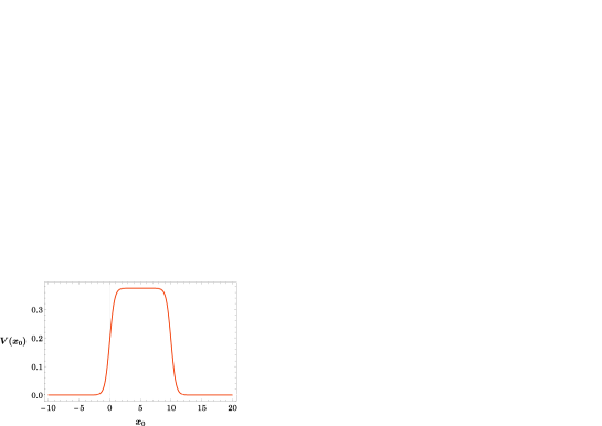
Figure 1: The potential $V(x_{0})$ that represents the presence of the curved region located between $x_{i}=0$ and $x_{f}=L=10$. The parameter $\varepsilon$ is equal to one.

The potential for this force represents the barrier associated with the curved region (Fig.1)

$$V(x_{0})=\varepsilon\frac{3}{4\pi}\,\Large[\arctan(\tanh(\frac{x_{0}-x_{i}}{2}))-\arctan(\tanh(\frac{x_{0}-x_{f}}{2}))+$$ (5)

$$\frac{1}{2}\,{\rm sech}(x_{0}-x_{i})\tanh(x_{0}-x_{i})-\frac{1}{2}\,{\rm sech}(x_{0}-x_{f})\tanh(x_{0}-x_{f})].$$

In this paper location of the inhomogeneity is assumed to be between $x_{i}=0$ and $x_{f}=L$.

In order to estimate the value of the critical speed that separates the kinks reflected from the barrier from those which pass over the barrier we separate the problem of movement in the barrier potential from the motion under the influence of constant force represented by constant bias current. The total energy of the kink that moves in the potential $V(x_{0})$ is $E=\frac{1}{2}m_{0}{u}^{2}+V(x_{0}),$ where kink mass is equal $m_{0}=8.$ At the beginning of its motion the kink moves almost freely having only kinetic energy

$$E_{in}=\frac{1}{2}m_{0}{u_{c}}^{2}.$$

We assume that at the end of its motion the kink stops on the top of the barrier having only the potential energy

$$E_{fin}=V(x_{0}=L/2)=\frac{32}{3\pi}~{}\varepsilon\left[2\arctan\left(\tanh\frac{L}{4}\right)+\mathrm{sech}\frac{L}{2}\tanh\frac{L}{2}\right].$$

The conservation of the energy leads to the following estimation of the critical velocity

$$u_{c}=\sqrt{\frac{8}{3\pi}~{}\varepsilon~{}}~{}\sqrt{2\arctan\left(\tanh\frac{L}{4}\right)+\mathrm{sech}\frac{L}{2}\tanh\frac{L}{2}}.$$ (6)

This estimation quite well describes the values of the critical velocity even in the case when the bias current and the dissipation term are taken into account. The reason for this is the fact that we work with velocities for which the bias current and dissipation almost cancel each other.

3 The influence of thermal fluctuations on the kink motion

Far from the barrier the last bracket from the right hand side of the equation (4) describes the residual interaction of the kink with the barrier (which is a consequence of the interaction of the kink tail with the curved region). We will describe how the fluxon approaching the barrier from the left, interacts with this barrier. This residual impact will be treated approximately as a position independent small interaction and therefore we consider the following equation

$$\dot{u}+\alpha u=\frac{2}{\pi}\,\Gamma-r,$$ (7)

instead of equation (4). Here $r$ is the above mentioned small residual interaction.

Our intention is to describe the influence of the nonzero temperature, of the system, on the process of overcoming the barrier by the fluxon. We assume that the bias current is a random variable i.e. it fluctuates due to the non-zero temperature of the system. The average value of the bias current we denote by $\Gamma_{0}$

$$<\Gamma(t)>=\Gamma_{0},$$ (8)

where averaging is with respect to all realizations of the thermal noise. In this situation from equation (7) we calculate the average value of the stationary speed (in stationary case $<\dot{u}>=0$)

$$u_{s}=\frac{2}{\pi\alpha}\,\Gamma_{0}-\frac{r}{\alpha},$$ (9)

where the average value of the stationary velocity is denoted by $u_{s}$. Moreover the thermal noise has the character of a white Gaussian noise and therefore the time correlation function of the bias current we assume in the form

$$<\Gamma(t)\Gamma(t^{\prime})>=A\delta(t-t^{\prime}).$$ (10)

In order to fix the appropriate value of the prefactor $A$ for the system in thermal equilibrium we came back to the equation (7). The solution of this equation under assumption of constant $r$ reads

$$u(t)=\frac{2}{\pi}\int_{0}^{t}dt^{\prime}\,\Gamma(t^{\prime})e^{\alpha(t^{\prime}-t)}-\frac{r}{\alpha}\,(1-e^{-\alpha t}).$$ (11)

Now we are ready to calculate the time correlation function of the velocity

$$<u(t)u(\bar{t})>=\left(\frac{2}{\pi}\right)^{2}\int_{0}^{t}dt^{\prime}\int_{0}^{\bar{t}}dt^{\prime\prime}<\Gamma(t^{\prime})\Gamma(t^{\prime\prime})>e^{\alpha(t^{\prime}+t^{\prime\prime}-t-\bar{t})}$$ (12)

$$-\frac{r}{\alpha}\,(1-e^{-\alpha\bar{t}})\frac{2}{\pi}\int_{0}^{t}dt^{\prime}<\Gamma(t^{\prime})>e^{\alpha(t^{\prime}-t)}-\frac{r}{\alpha}\,(1-e^{-\alpha t})\frac{2}{\pi}\int_{0}^{\bar{t}}dt^{\prime}<\Gamma(t^{\prime})>e^{\alpha(t^{\prime}-\bar{t})}$$

$$+\left(\frac{r}{\alpha}\right)^{2}(1-e^{-\alpha\bar{t}})(1-e^{-\alpha t})$$

If we apply formulas (8) and (10) for average and the time correlation of the bias current, and moreover assume $t=\bar{t}$ then we obtain

$$<u(t)^{2}>=<u(t)u(\bar{t})>_{\bar{t}=t}=\frac{2A}{\pi^{2}\alpha}\,(1-e^{-2\alpha t})+\left[\left(\frac{r}{\alpha}\right)^{2}-\frac{4\Gamma_{0}}{\pi\alpha^{2}}\,r\right](1-e^{-\alpha t})^{2}.$$ (13)

The system after the required length of time tends to thermodynamic equilibrium and therefore we extract in the last formula the terms that dominate long time behaviour of $<u^{2}>$

$$<u(t)^{2}>=\frac{2A}{\pi^{2}\alpha}+\left(\frac{r}{\alpha}\right)^{2}-\frac{4\Gamma_{0}}{\pi\alpha^{2}}\,r.$$ (14)

The kinetic energy of the fluxon after a sufficiently long time reads

$$E_{k}=\frac{1}{2}\,m<u(t)^{2}>=\frac{1}{2}\,m\left[\frac{2A}{\pi^{2}\alpha}+\left(\frac{r}{\alpha}\right)^{2}-\frac{4\Gamma_{0}}{\pi\alpha^{2}}\,r\right],$$ (15)

where $m$ is kink mass. We expect that after an appropriately long time the system tends to thermal equilibrium. On the other hand in thermodynamic equilibrium, on the basis of the equipartition principle, it is proportional to the temperature $T$

$$E_{k}=\frac{1}{2}\,kT,$$ (16)

here $k$ is Boltzmann constant. Comparison of the equations (15) and (16) allows the determination of the coefficient $A$

$$A=\frac{\pi^{2}\alpha k(T-\Delta T)}{2m},$$ (17)

where we denoted

$$\Delta T\equiv\frac{m}{k}\left[\left(\frac{r}{\alpha}\right)^{2}-\frac{4\Gamma_{0}}{\pi\alpha^{2}}\,r\right].$$ (18)

For further convenience, we transform the formula (18) to the form containing the critical value of the bias current $\Gamma_{c}$

$$\Delta T=\Omega(\Gamma_{c}-\Gamma_{0})-\omega.$$ (19)

This critical value $\Gamma_{c}$ separates the values of the bias current for which the particle passes over the barrier from the values for which the reflection occurs. The parameters in the above formula are defined as follows

$$\omega\equiv\frac{m}{k}\left[\frac{4\Gamma_{c}}{\pi\alpha^{2}}\,r-\left(\frac{r}{\alpha}\right)^{2}\right],\,\,\,\,\Omega\equiv\frac{4m}{\pi\alpha^{2}k}.$$

Finally, the average and the time correlation function of bias currents are defined by the formulas

$$<\Gamma(t)>=\Gamma_{0},\,\,\,<\Gamma(t)\Gamma(t^{\prime})>=\frac{\pi^{2}\alpha k(T-\Delta T)}{2m}\,\delta(t-t^{\prime}).$$ (20)

The equations (20) are the starting point for the derivation of the Fokker - Planck equation described in appendix A. The stationary solution of this equation is the following

$$P(u)=\sqrt{\frac{m}{2\pi k(T-\Delta T)}}\exp\left(-\frac{m}{2k(T-\Delta T)}\,(u-u_{s})^{2}\right).$$ (21)

This probability is a base for calculation of the total probability of the transmission of the kink through the potential barrier. We have to deal with the transition event whenever the kink speed exceeds the critical velocity

$$\Delta P=\int_{u_{c}}^{\infty}duP(u)=\frac{1}{2}\,\mathrm{erf}\left(\sqrt{\frac{m}{2k(T-\Delta T)}}\mid u_{c}-u_{s}\mid\right),$$ (22)

in this formula $\mathrm{erf}$ denotes an error function. This probability depends, in addition to temperature and residual effects, on the difference of critical $u_{c}$ and stationary $u_{s}$ velocities in the system. The critical velocity separates two regimes. In the first regime the particle passes over the barrier and in the second it reflects from the barrier.

The probabilities obtained on the basis of the field model and analytical result (22) based on the Foccker - Planck approach are compared in Figures 3-5 for different ranges of temperatures. Due to potential applications also in high-temperature superconductors, the comparison was made for intervals from zero to $T=50K$, $T=20K$ and $T=5K$. In all plots the parameters of the shift $\Delta T$ given in the formula (19) are fitted so that they take the values $\Omega=25220.6$ and $\omega=-0.398529$. We decided to fit these parameters because the residual interaction is out of our control. Starting from the field model we obtain the fit of $\Delta T$ as a function of the absolute value of separation between actual average value of the bias current and its critical value. This fit is presented in Figure 2.

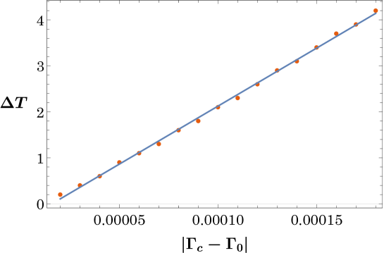
Figure 2: $\Delta T$ as a function of modulus of difference of the critical value of the bias current and actual average of the bias current. The parameters of the fit are $\Omega=25220.6$ and $\omega=-0.398529$.

In all simulations we assume damping coefficient on the level of $\alpha=0.01$. Moreover we assumed the size of the inhomogeneity $L=10$ and we located its position between $x_{i}=0$ and $x_{f}=10$. The the strength of the heterogeneity is fixed at the level of $\varepsilon=1$. Because a relativistic formula (44) for stationary speed is known therefore we use it in all plots (see Appendix C). On the other hand in Figures 3-4 the critical velocity is approximated by the non-relativistic formula (6).

Figure 3: The probability of transition of the fluxon obtained from the field model compared in the interval $T\in[0K,50K]$ with the analytical formula. The parameters of the plots are $\alpha=0.01$, $\varepsilon=1$, $L=10$. The blue line and points correspond to the bias current exceeding its critical value and the red to the bias current below its critical value.

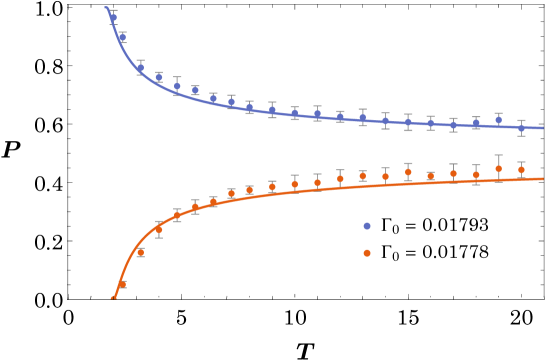
Figure 4: The probability of transition of the fluxon in the interval $T\in[0K,20K]$. Comparison of the analytical result with the field model prediction. The parameters of the plots are $\alpha=0.01$, $\varepsilon=1$, $L=10$. The blue line and points represents data for the bias current exceeding its critical value and the red ones the bias current below its critical value.

This choice is motivated by the fairly good compatibility of the approximated formula with the results obtained on the background of the field model. On the other hand in the case of Figure 5 the accuracy of the formula (6) was insufficient and therefore we used the relativistic model (40) obtained in appendix B.

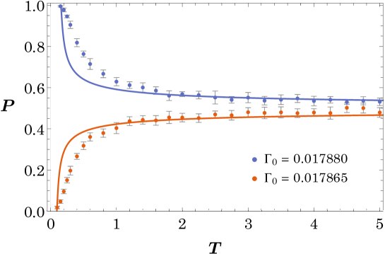
Figure 5: Transition probability of the fluxon in the interval $T\in[0K,5K]$. The parameters of the plots are $\alpha=0.01$, $\varepsilon=1$, $L=10$. The blue line and points correspond to the bias current exceeding its critical value and the red ones to the bias current below its critical value.

The figures show that for the bias currents above the critical value (blue line for analytical formula and points for the field model), as the temperature increases, the probability of the particle passing over the barrier decreases. The reduction of transition probability is in the direction of the value of one-half, the achievement of which would make such a process completely random. On the other hand, for the bias currents below its critical value (red line for the formula and points for the field model) as the temperature increases, the probability of the particle passing over the barrier also increases. The probability increases gradually towards the half value beyond which the process would be completely random. The comparison of the results of the field model in nonzero temperature with analytical description provided by formula (22) shows a pretty good level of compatibility. The results are consistent in Figures 3 and 4, while in Figure 5 there are deviations below one Kelvin. Figures 3-5 show simulations when the currents slightly differ from the critical current. On the other hand, if the difference between the average bias current and its critical value is significant, then thermal fluctuations have a negligible impact on the process of interaction between the kink and the curved region. In this case the interaction is properly described by a deterministic model i.e. if the bias current is below the value of critical current then the kink is reflected from the curved region. On the other hand if bias current exceeds its critical value then the kink goes through the curved region. This behaviour is crucial for possible technical applications.

4 Remarks

In the present article we considered the impact of thermal fluctuations on the process of interaction of the kink with the heterogeneous region of the system described by a nearly integrable sine-Gordon model. The physical background of the studies is the influence of the curvature on the fluxon motion in the long Josephson junction. We obtained analytical formulas that describe probabilities of transition through and reflection of the kink from the potential barrier that represents heterogeneity. The main result is based on the Foccker - Planck equation obtained for the considered system. We compared the analytical results with the simulations performed in the framework of the field model for different ranges of temperatures. Due to potential applications in normal and also in high-temperature superconductors, the comparison was made for intervals from zero to $T=50K$, $T=20K$ and $T=5K$. The compatibility of the analytical formula with the numerical simulations is satisfactory in the first (Fig.3) and the second regime (Fig.4). In the third regime (Fig.5) the compliance above one $1K$ is also satisfactory.

The most problematic regime of temperature is presented in figure 5. In this interval we resigned from the formula (6) for critical velocity and in order to obtain a better fit we used the relativistic model (40) for estimation of the critical speed. Either way we observed in the small temperature regime presented in Figure 6 some discrepancy between the result of the field model and our fit located in the interval from $0K$ to $1K$. We identified a probable reason for this problem.

In the low temperature regime we observed occurrence of the resonance windows in the transition process. It means that we observe very narrow regimes of the parameters that corresond to transition below the critical speed and moreover the reflection regimes above the critical velocity. This phenomenon has a place in the effective model (40) and in the original field model (1) as well. This phenomenon is responsible for the ambiguity of the estimation of the critical speed and is responsible for the discrepancy of the approximate description and the results of the field model in Fig.6. A similar phenomenon was previously observed by many researchers. For example in article [23] in the $\phi^{4}$ model an interaction of the kink with attracting point impurity was studied. The existence of resonance windows in initial speeds below some threshold velocity had found an explanation in the resonant energy exchange between the kink internal mode and its translational mode. This behaviour was first observed numerically by Campbell [24] and his collaborators in the case of kink-antikink scattering in the $\phi^{4}$ model. Presently there is a variety of articles that contain a detailed explanation of the two-bounce resonance observed in kink - antikink collisions [25]. A separatrix map for this problem that explains the complex fractal-like dependence on initial velocity for kink-antikink collisions was also constructed. The chaotic nature of such collisions depends on the transfer of energy to a secondary mode of oscillation [26]. In the frame of the moduli space formalism [27] a spectacular result in reproducing the fractal structure in the formation of the final state was reached in article [28]. The key insight of these articles is that the existence of resonance windows is possible due to the presence of an internal mode in the spectrum of the kink in the $\phi^{4}$ model [29, 30]. The situation in the case of the sine-Gordon model is different. The linear spectra of the kink excitations does not contain the discrete internal mode and therefore the structure and the nature of the windows in the model considered in this paper is enigmatic. On the other hand the modification of the sine-Gordon model considered in this article belongs to the so called nearly integrable variations of the original model. The studies on this subject are ongoing and will be presented in the future. To some degree a similar example of the model containing resonance windows in kink-antikink interactions was presented in the article [31]. This article describes the solutions of the $\phi^{6}$ model that does not contain, in its linear spectra of excitations, the discrete internal eigenmodes which, to some degree, resembles our system.

5 Acknowledgements

This research was supported in part by PLGrid Infrastructure.

6 Appendix A: Fokker - Planck equation

For the sake of completeness of the article we present derivation of the Fokker - Planck equation for the system studied by us. First, let us notice that velocity variation is a random variable with the following mean value

$$<\delta u>=<\dot{u}\,\delta t>=(-\alpha u-r+\frac{2}{\pi}\,\Gamma_{0})\,\delta t,$$ (23)

where we used formula (7) and bias current mean value (8). Similarly, formula (20) leads to the expression

$$<\delta u\delta u>=\frac{2\alpha k(T-\Delta T)}{m}\,\delta t.$$ (24)

Next the conditional probability that the particle which has velocity $u$ at time $t+\delta t$, a moment earlier i.e. at $\bar{t}$, had velocity $\bar{u}$ we denote by $P(u,t+\delta t;\bar{u},\bar{t})$. Taylor expansion of this probability with respect to final time reads

$$P(u,t+\delta t;\bar{u},\bar{t})=P(u,t;\bar{u},\bar{t})+\partial_{t}P(u,t;\bar{u},\bar{t})\delta t,$$ (25)

where we ignored the terms of second and higher orders in $\delta t$. On the other hand we can obtain this expansion starting from the Chapman - Kolmogorov equation

$$P(u,t+\delta t;\bar{u},\bar{t})=\int_{-\infty}^{+\infty}du^{\prime}P(u,t+\delta t;u^{\prime},t^{\prime})P(u^{\prime},t^{\prime};\bar{u},\bar{t}),$$ (26)

which states that, at some intermediate time $\bar{t}<t^{\prime}<t+\delta t$ the velocity $u^{\prime}$ belongs to the interval $u^{\prime}\in(-\infty,+\infty)$. The probability present in this formula can be expressed with the velocity variation $\delta u$ as follows

$$P(u,t+\delta t;u^{\prime},t^{\prime})=<f(u-u^{\prime}-\delta u>,$$ (27)

which can be expanded with respect to velocity

$$P(u,t+\delta t;u^{\prime},t^{\prime})=f(u-u^{\prime})+<\delta u>\partial_{u^{\prime}}f(u-u^{\prime})+\frac{1}{2}\,<\delta u\,\delta u>\partial_{u^{\prime}}^{2}f(u-u^{\prime}).$$ (28)

Truncation at the second order is motivated by the fact that they contain at most linear terms in $\delta t$. The Chapman - Kolmogorov formula now reads

$$P(u,t+\delta t;\bar{u},\bar{t})=\int_{-\infty}^{+\infty}du^{\prime}[f(u-u^{\prime})+$$ (29)

$$<\delta u>\partial_{u^{\prime}}f(u-u^{\prime})+\frac{1}{2}\,<\delta u\,\delta u>\partial_{u^{\prime}}^{2}f(u-u^{\prime})]P(u^{\prime},t^{\prime};\bar{u},\bar{t}),$$

Assuming that $f$ and its first derivative disappear at plus/minus infinity and integrating second and third terms by parts we obtain

$$P(u,t+\delta t;\bar{u},\bar{t})=\int_{-\infty}^{+\infty}du^{\prime}f(u-u^{\prime})[P-\partial_{u^{\prime}}(<\delta u>P)+\frac{1}{2}\,<\delta u\,\delta u>\partial_{u^{\prime}}^{2}P],$$ (30)

where we have used the fact that $<\delta u\,\delta u>$ does not depend on $u$. From formulas (23) and (24) it is also transparent that the last two terms are linear in $\delta t$. Let us also notice that without random variation $\delta u$ the probability distribution is unambiguously determined as follows $f(u-u^{\prime})=\delta(u-u^{\prime})$ and therefore after integration we obtain

$$P(u,t+\delta t;\bar{u},\bar{t})=P(u,t;\bar{u},\bar{t})-\partial_{u}\left(<\delta u>P(u,t;\bar{u},\bar{t})\right)+$$ (31)

$$\frac{1}{2}\,<\delta u\delta u>\partial_{u}^{2}P(u,t;\bar{u},\bar{t}).$$

Next we replace the average and variance of the random variable $\delta u$ from formulas (23), (24) and we obtain

$$P(u,t+\delta t;\bar{u},\bar{t})=P(u,t;\bar{u},\bar{t})+\partial_{u}\left((\alpha u+r-\frac{2}{\pi}\,\Gamma_{0})P(u,t;\bar{u},\bar{t})\right)\delta t+$$ (32)

$$\frac{\alpha k(T-\Delta T)}{m}\,\partial_{u}^{2}P(u,t;\bar{u},\bar{t})\delta t.$$

Finally, comparison of the above formula with equation (25) leads to the following form of the Fokker - Planck equation for the system considered by us

$$\partial_{t}P=\partial_{u}\left((\alpha u+r-\frac{2}{\pi}\,\Gamma_{0})P+\frac{\alpha k(T-\Delta T)}{m}\,\partial_{u}P\right).$$ (33)

The time independent ($\partial_{t}P=0$) normalized solution of this equation reads

$$P(u)=\sqrt{\frac{m}{2\pi k(T-\Delta T)}}\exp\left(-\frac{m}{2k(T-\Delta T)}\,(u-u_{s})^{2}\right),$$ (34)

where we used (9) in order to identify the presence of the average stationary velocity $u_{s}$ in the equation.

7 Appendix B: Effective relativistic description of the kink

In order to obtain a relativistic approximation of the critical speed of the kink we reconsider the projection procedure onto the energy density used in Section 2. We start again with the field equation

$$\partial_{t}^{2}\phi+\alpha\partial_{t}\phi-\partial_{x}({\cal F}(x)\partial_{x}\phi)+\sin\phi=-\Gamma_{0}.$$ (35)

Similarly as before we introduce the kink like ansatz into the field equation

$$\phi(t,x)=4\arctan(e^{\xi(t,x)}),$$

where this time the function $\xi$ takes its relativistic form

$$\xi=\gamma(t)(x-x_{0}(t)).$$

Moreover, the function ${\cal F}$ is expressed by the auxiliary function $g(x)$

$${\cal F}(x)=1+\varepsilon g(x),$$

where dimensionless parameter $\varepsilon$ controls the magnitude of curvature. Next we insert the kink ansatz into the field equation (35), obtaining

$$\left[\left(\frac{\ddot{\gamma}}{\gamma}+\alpha\frac{\dot{\gamma}}{\gamma}\right)\xi-(2\dot{\gamma}u+\gamma\dot{u}+\alpha\gamma u)\right]\textrm{~{}sech}\xi+$$

$$\left[(\gamma^{2}-1-\dot{\gamma}^{2}u^{2})+2\dot{\gamma}u\xi-\left(\frac{\dot{\gamma}}{\gamma}\right)^{2}\xi^{2}\right]\mathrm{sech}\xi\tanh\xi-$$ (36)

$$\varepsilon\gamma(\partial_{x}g)~{}\mathrm{sech}\xi+\varepsilon\gamma^{2}g(x)~{}\mathrm{sech}\xi\tanh\xi=-\frac{1}{2}\Gamma_{0}.$$

We eliminate the spatial variable from the description by projection onto the energy density distribution

$$Eq=0\Rightarrow\int_{-\infty}^{+\infty}dx\textrm{~{}sech}^{2}\xi\,Eq=0.$$ (37)

As a result of this procedure, we obtain a one-dimensional relativistic model describing the location of the kink

$$\dot{u}+\alpha u+\frac{4}{3}~{}u\frac{\dot{\gamma}}{\gamma}=\frac{4}{3\pi}~{}\varepsilon\gamma\left(\mathrm{sech}^{3}\xi_{L}-\mathrm{sech}^{3}\xi_{0}\right)+\frac{2}{\pi\gamma}~{}\Gamma_{0},$$ (38)

where we denoted $\xi_{L}=\gamma(L-x_{0}(t))$ and $\xi_{0}=\gamma(-x_{0}(t)).$ On the other hand, introducing to the last equation the Lorentz factor $\gamma=1/\sqrt{1-u^{2}}$ (we use the units with Swihart velocity equal to one $c=1$) we obtain

$$\left(1+\frac{1}{3}~{}u^{2}\right)\dot{u}+\alpha u(1-u^{2})=\frac{4}{3\pi}~{}\varepsilon\sqrt{1-u^{2}}\left(\mathrm{sech}^{3}\xi_{L}-\mathrm{sech}^{3}\xi_{0}\right)+\frac{2}{\pi}(\sqrt{1-u^{2}})^{3}~{}\Gamma_{0}.$$ (39)

This equation is a base for estimation of the critical speed in our system in the low temperature regime presented in Fig. 5.

8 Appendix C: Relativistic approximation of the stationary speed

For the sake of completeness of the presentation, we will also recall the origin and the relativistic value of the kink stationary speed used in this work. The bias current and dissipation present in the system have an opposite effect on fluxon motion leading to mutual equilibration at a certain speed [32]. The dynamics of the soliton in the homogenous system is described by the equation

$$\partial_{t}^{2}\phi+\alpha\,\partial_{t}\phi-\partial_{x}^{2}\phi+\sin\phi=-\Gamma_{0}.$$ (40)

If we multiply both sides of this equation by the time derivative of the field $\phi$ and next integrate it with respect to the space variable, then we obtain

$$\frac{d}{dt}H^{SG}=-\int_{-\infty}^{+\infty}dx\left[\Gamma_{0}\,\partial_{t}\phi+\alpha\,(\partial_{t}\phi)^{2}\right],$$ (41)

where $H^{SG}$ is the hamiltonian of the sine-Gordon model

$$H^{SG}=\int_{-\infty}^{+\infty}dx\left[\frac{1}{2}(\partial_{t}\phi)^{2}+\frac{1}{2}(\partial_{x}\phi)^{2}+(1-\cos\phi)\right].$$

Introducing the kink ansatz

$$\phi(t,x)=4\arctan\left(\frac{x-x_{0}-ut}{\sqrt{1-u^{2}}}\right)$$

into equation (42) leads to the ordinary differential equation for the fluxon velocity

$$\frac{du}{dt}=\frac{1}{4}\,\pi\Gamma_{0}(1-u^{2})^{\frac{3}{2}}-\alpha\,u(1-u^{2}).$$ (42)

The constant equilibrium $(du/dt=0)$ solution of this equation, corresponds to the situation when the power input caused by the bias current is is balanced by the loss of power due to dissipation

$$u_{s}=\frac{1}{\sqrt{1+(\frac{4\alpha}{\pi\Gamma_{0}})^{2}}}~{}.$$ (43)

This velocity describes the stationary motion of the fluxon in the homogeneous junction.

References

- [1] B. D. Josephson, Phys. Lett. 1, 251 (1962).
- [2] B. D. Josephson, Rev. Mod. Phys. 46, 251 (1974).
- [3] . P. W. Anderson, J. M. Rowell, Phys. Rev. Lett. 10, 230 (1963).
- [4] Applied Superconductivity: Handbook on Devices and Applications, P. Seidel (ed.), Wiley, ISBN 13: 978-3-27-741209-9 (2015).
- [5] A. I. Braginski, J Supercond. Nov. Magn. 32, 23 (2019).
- [6] J. G. Bednorz and K. A. Müller, Z. Phys. B 64, 189 (1986).
- [7] A. Schilling, M. Cantoni, J. D. Guo, and H. R. Ott, Nature 363, 56 (1993).
- [8] A. Benabdallah, J. G. Caputo, and A. C. Scott, Phys. Rev. B 54, 16139 (1996).
- [9] A. Kemp, A. Wallraff, and A. V. Ustinov, Phys. Stat. Sol. B 233, 472 (2002).
- [10] A. Kemp, A. Wallraff, and A.V. Ustinov, Physica C 368, 324 (2002).
- [11] D. R. Gulevich and F. V. Kusmartsev, Phys. Rev. Lett. 97, 017004 (2006).
- [12] D. R. Gulevich, F. V. Kusmartsev, S. Savelev, V. A. Yampolśkii, and F. Nori, Phys. Rev. Lett. 101, 127002 (2008).
- [13] J.G. Caputo and D. Dutykh, Phys. Rev. E 90, 022912 (2014).
- [14] R. Monaco, J. Phys. Condens. Matter 28, 445702 (2016).
- [15] R. Monaco, J. Mygind, and V. P. Koshelets, Supercond. Sci. Technol. 31, 025003 (2018).
- [16] T. Dobrowolski and A. Jarmoliński, Phys. Rev. E 101, 052215 (2020).
- [17] T. Dobrowolski, Phys. Rev. E 79, 046601 (2009).
- [18] T. Dobrowolski, Discrete Contin. Dyn. Syst. Ser. S 4, 1095 (2011).
- [19] T. Dobrowolski, Ann. Phys. (N.Y.) 327, 1336 (2012).
- [20] T. Dobrowolski, Eur. Phys. J. B 86, 346 (2013).
- [21] T. Dobrowolski and A. Jarmoliński, Phys. Rev. E 96, 012214 (2017).
- [22] J. Gatlik and T. Dobrowolski, Physica D 428, 133061 (2021).
- [23] Z. Fei, Y. S. Kivshar, and L. Vazquez, Phys. Rev. A 46, 5214 (1992).
- [24] D. K. Campbell, J. F. Schonfeld, and C.A. Wingate, Physica D 9, 1 (1983).
- [25] R.H. Goodman and R. Haberman, SIAM J. Appl. Dyn. Syst. 4, 1195 (2005).
- [26] R.H. Goodman, Chaos 18, 023113 (2008).
- [27] N. S. Manton, K. Oleś, T. Romańczukiewicz, and A. Wereszczyński Phys. Rev. D 103, 025024 (2021).
- [28] C. Adam, N. S. Manton, K. Oleś, T. Romańczukiewicz, and A. Wereszczyński, Phys.Rev. D 105, 065012 (2022).
- [29] I. Takyi and H. Weigel, Phys. Rev. D 94, 085008 (2016).
- [30] P. G. Kevrekidis and R. H. Goodman, arXiv:1909.03128v1 (2019).
- [31] P. Dorey, K. Mersh, T. Romańczukiewicz, and Y. Shnir, Phys. Rev. Lett. 107, 091602 (2011).
- [32] D.W. McLaughlin and A.C. Scott, Phys. Rev. A 18, 1652 (1978).