Complex Networks Analysis of the Energy Landscape of the Low Autocorrelation Binary Sequences Problem

Abstract

We provide an up-to-date view of the structure of the energy landscape of the low autocorrelation binary sequences problem, a typical representative of the $NP$-hard class. To study the landscape features of interest we use the local optima network methodology through exhaustive extraction of the optima graphs for problem sizes up to $24$. Several metrics are used to characterize the networks: number and type of optima, optima basins structure, degree and strength distributions, shortests paths to the global optima, and random walk-based centrality of optima. Taken together, these metrics provide a quantitative and coherent explanation for the difficulty of the low autocorrelation binary sequences problem and provide information that could be exploited by optimization heuristics for this problem, as well as for a number of other problems having a similar configuration space structure.

1 Introduction

Given a binary sequence $s=(s_{1},s_{2},\ldots,s_{N})$ of length $N$ with $s_{i}\in\{-1,+1\}$, the autocorrelation of $s$ is defined as:

$$C_{k}(s)=\sum_{i=1}^{N-k}s_{i}s_{i+k}$$

The Energy $E$ of the sequence $s$ is then given by:

$$E(s)=\sum_{k=1}^{N-1}C_{k}^{2}(s),$$

and the Merit Factor $F(s)$ of $s$ has the form:

$$F(s)=\frac{N^{2}}{2E(s)}$$

Binary sequences of this type with minimal, or low, autocorrelation arise in several areas, especially in telecommunications, but also in mathematics, statistical physics, and criptography. Although we shall not comment on these important theoretical and applied fields, limiting our work to the combinatorial optimization aspects, the following references should be helpful [1, 2, 3]. The algorithmic goal is to minimize $E$ or, equivalently, to maximize $F$ and we shall call the optimization problem the LABS (Low Autocorrelation Binary Sequences) problem for a given sequence $s$. The problem becomes exponentially harder as $N$ increases since the number of admissible solutions grows as $2^{N}$ and thus the time complexity in the worst case correspondingly grows as $O(2^{N})$. In fact, no algorithm other than complete enumeration or its variants, such as branch-and-bound, is known for the problem, which therefore belongs to the $NP$-hard class.

LABS configurations enjoy a number of symmetries [4]. Among them, simply reversing or complementing a binary string leaves the energy invariant. Because of these symmetries ground and higher states of the system are always degenerate, i.e., there is more than one state with the same energy. An important subset of sequences of odd length $N$ are called skew-symmetric if they satisfy $s_{j+l}=(-1)^{l}\>s_{j-l}$. Because only one half of the sequence is required, this reduces the search space size from $2^{N}$ to $2^{N/2}$ and thus makes the problem less computationally intensive if minimum energy sequences are skew-symmetric [4].

Global optimal configurations for $N$ up to $66$ have been found by exhaustive enumeration using branch-and-bound techniques [4]. For larger $N$ a number of heuristic stochastic techniques have been used, including simulated annealing, tabu search, and evolutionary algorithms among others. Using these approaches that cannot guarantee global optimality, best, but not necessarily globally optimal solutions, have been found for many large odd $N$ values up to approximately $N=400$ [5]. In fact, an empirical upper bound of about $12$ for $F(s)$ has been given by Golay [1], but for large $N$ there is a gap between the largest $F$ found and the bound [4] which means that it is likely that these current best sequences are not globally optimal.

The LABS problem has a strong link with spin systems in statistical mechanics. In fact, LABS is formally similar to a long-range four-spin spin glass model [6] but it is completely deterministic and has no quenched disorder. Because of this similarity, the model has been intensively studied with the methods of statistical mechanics thereby producing many useful results (see, e.g., [6, 2, 7]). The common features of these problems is the presence of frustration, which causes the system to get stuck into suboptimal states from which it is difficult to escape. However, we shall not pursue this direction further here. Instead, in the present study we shall focus on an aspect of the LABS problem that has been less investigated: the analysis of the structure of the energy landscape. This is very important to get a better understanding of what type of heuristics are likely to be more efficient for searching the problem space, given that complete enumeration is out of the question for $N$ sufficiently large. To our knowledge, there is only a previous study by Ferreira et al. [8] of the LABS energy landscape using the concept of barrier trees and the notions of depth and difficulty. Our goal in the present contribution is to deepen our understanding of the energy landscape of the LABS problem beyond that offered by [8] and, at the same time, uncover a number of features that are common to most hard combinatorial optimization problems that have fitness landscapes similar to the LABS landscape. In order to investigate the global structure of the energy landscape we shall use an approach based on Local Optima Networks (LONs) previously developed in our group [9] in which the $2^{N}$ original configurations are reduced to those that are local optima and to their connexions only. It has been shown in a number of works that the LON approach is a valuable one and, by studying the corresponding graph with the methods of complex networks, it can give useful insights on the factors causing the hardness of many combinatorial problems, see e.g., [9, 10].

The rest of the article is structured as follows. For the sake of self-containedness, in the next section we present the main ideas of Local Optima Networks (LONs). This is followed by the analysis of the exhaustive LONs generated by LABS instances of size $N$ for $N$ up to $24$. The results are then discussed in terms of the relationship between fitness landscape structure and problem difficulty. Finally, we present our conclusions.

2 Fitness Landscapes and Local Optima Networks

Let us consider a discrete problem $\mathcal{P}$ and an instance $\mathcal{I}_{\mathcal{P}}$ of $\mathcal{P}$. $I_{\mathcal{P}}$’s fitness landscape [11] is a triplet $({\cal X},{\cal N},f)$ where ${\cal X}$ is a set of admissible solutions, i.e., a search space; ${\cal N}:{\cal X}\longrightarrow 2^{\cal X}$, a neighborhood structure; that is, a function that assigns to every $x\in{\cal X}$ a set of neighbors ${\cal N}(x)$, and $f:{\cal X}\longrightarrow\mathbb{R}$ is a fitness function that provides the fitness, or objective value, of each $x\in{\cal X}$. In the LABS case fitness is sinonymous with the energy of a given binary sequence and the set of admissible solutions ${\cal X}$ is the set of all possible binary sequences of length $N$ formed with the symbols $\{-1,1\}$. The neighborhood ${\cal N}(x)$ of a solution $x$ can be defined in various ways. Here we use the standard 1-bit flip operator that changes the sign of single digit in the sequence $x$ so that $|{\cal N}(x)|=N$. The elements $x$ of ${\cal X}$ are related to the ordinary Boolean hypercube with elements $b_{i}\in\{0,1\}$ by the transformation $x_{i}=2b_{i}-1$.

The LON idea [9, 12, 13] starts from the above concepts and builds a new graph $G_{w}=(V,E)$ in which $V$ is the set of vertices which are local optima in the given fitness landscape and $E$ is the set of arcs joining two given vertices when they are directly reachable from each other in a sense that will be made explicit below. We now explain the construction of the graph $G_{w}$ in more detail.

The nodes $V$ in the network are local optima (LOs) in the search space. For a minimization problem, a solution $x\in{\cal X}$ is a local optimum iff $\forall x^{\prime}\in{\cal N}(x)$, $f(x^{\prime})\geqslant f(x)$. For a maximization problem the inequality is reversed. LOs are extracted using a best-improvement descent local search, as given in Algorithm 1 in which when selecting the fittest neighbor (line 4), ties are broken at random.

1:procedure Local Descent

2:     $x\leftarrow$ random initial solution

3:     while $x\not=$ Local Optimum do

4:         set $x^{\prime}\in{\cal N}(x)$, s.t. $f(x^{\prime})=min_{y\in{\cal N}(x)}f(y)$

5:         if $f(x)\leq f(x^{\prime})$ then

6:              $x\leftarrow x^{\prime}$

7:         end if

8:     end while

9:end procedure

Algorithm 1 Best-improvement local descent (bild)

The edges $E$ in the network are defined according to a distance function $dist$ and a positive integer $D>0$. The distance function represents the minimal number of moves between two solutions by a given search (mutation) operator which is a one-bit flip in our case. There is an edge $e_{ij}$ between local optima $LO_{i}$ and $LO_{j}$ if a solution $x$ exists such that $dist(x,LO_{i})\leqslant D$ and $bild(x)=LO_{j}$. In other words, if $LO_{j}$ can be reached after mutating $LO_{i}$ and running best improvement local descent from the mutated solution. The weight $\tilde{w}_{ij}$ of this edge is $\tilde{w}_{ij}=\sharp\{x\in{\cal X}~{}|~{}dist(x,LO_{i})\leqslant D\mbox{ and }bild(x)=LO_{j}\}$. That is, the number of $LO_{i}$ mutations that reach $LO_{j}$ after local descent. This weight can be normalized by the total number of solutions, $\sharp\{x\in{\cal X}~{}|~{}dist(x,LO_{i})\leqslant D\}$, within reach at distance $D$: $w_{ij}=\tilde{w}_{ij}/\sum_{j}\tilde{w}_{ij}$.

Summarizing, the LON is the weighted graph $G_{w}=(V,E)$ where the vertices $v_{i}\in V$ are the local optima, and there is an edge $e_{ij}\in E$, with weight $w_{ij}$, between two vertices $v_{i}$ and $v_{j}$ if $w_{ij}>0$. According to the definition of weights, $w_{ij}$ may be different than $w_{ji}$. Thus, two weights are needed in general, and $G_{w}$ is a weighted, directed transition graph.

The above systematic construction is only possible for problem instances of small to medium size. For larger instances it is possible to resort to reliable sampling techniques, for instance as described in [14]. In the present work the problem sizes considered have allowed us to use exhaustive enumeration.

To give an idea of how a LON looks like, the following Fig. 1 depicts the LABS LON for $N=8$. For $N>10$ the graphs become too dense and direct visualization is not useful. By the way, we note that the ratio of the total number of optima to the number of global optima in this small LON is $1.5$ but it quickly increases with increasing $N$ (see Sect. 4). To analyze the network structure in the general case it is better to resort to relevant graph metrics that summarize important graph features in a single number, a few numbers, or a probability distribution. This is the goal of the next section.

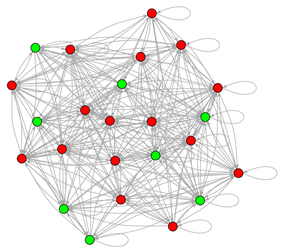
Figure 1: The Local Optima Network of the LABS problem with $N=8$. Directed weighted edges stand for transitions frequencies between the basins corresponding to the minima nodes. Self-loops represent the fraction of transitions that remain in the source basin. Here edge weights are drawn equal for the sake of clarity. Global minima are in red. The other local optima are in green.

We also mention that LONS can be seen as the discrete equivalent of the inherent structures of the free or potential energy hypersurfaces in the continuous parameter spaces of chemical-physical systems such as macromolecules and atom clusters [15].

3 LON Metrics

Once we have built a LON, we are in a position of using tools from the science of complex networks to analyze the corresponding graphs. There exist many metrics for describing complex networks. Among them, the following ones are those that have proved useful in characterizing the difficulty of problem instances through their corresponding LONs in previous work [9, 12]. They are briefly defined here for the sake of self-containedness, more details can be found, for example, in the books [16, 17].

Network size.

The number of vertices in the LON and its variation with $N$ gives information about the difficulty for a searcher to find the global optimum. It also provides data on the sizes of the associated attraction basins.

Strength.

This term refers to the generalization of the vertex degree to weighted networks. It is defined as the sum $s_{i}$ of weights of the edges from node $i$ to its neighbors ${\cal N}(i)$,

$$s_{i}=\sum_{j\in{\cal N}(i)}w_{ij},$$

where $w_{ij}$ is the weight of the edge connecting nodes $i$ and $j$. For directed graphs one speaks of outgoing strength which is computed on the edges outgoing from the node while incoming strength refers to incoming edges.

Degree, strength, and edge weight distribution functions.

These discrete distributions give, respectively, the frequency of a given node degree, node strength, or edge weight in the network. These distributions are useful for evaluating whether they are, for instance, homogeneous or heterogeneous, unimodal or multimodal.

Average shortest paths.

The average value $\langle L\rangle$ of all two-point shortest paths in a graph give an idea of the typical distances between nodes. It is given by:

$$\langle L\rangle=\frac{2}{N(N-1)}\sum_{i=1}^{N}\sum_{j>i}l_{ij}.$$

Where $l_{ij}$ is the shortest path between vertices $i$ and $j$. In LON networks edges are directed and weighted and thus Dijkstra’s algorithm is usually employed to compute them. These paths always exist because complete LONs are strongly connected.

Network centrality.

Centrality measures of various kinds are often used, especially in social networks, to characterize actors that are centrally located in some specified sense. Centrality can also be used in other contexts and we shall use PageRank here to investigate the centrality of optima in a LON graph.

4 Results

In this section we show and discuss the main results obtained by constructing and analyzing the full LONs for LABS problems with size $N$ in the range $3$ to $24$. We remark that, in contrast with classical combinatorial problems such as QAP or TSP, or spin glasses with quenched disorder in which many different instances can be generated for a given size $N$, LABS, being completely deterministic, has only one instance for each problem size $N$ with the vertices of the $N$-ary hypercube $\{-1,1\}^{N}$ as admissible solutions. This feature does not allow to take averages over a sample of instances as in the other cases.

4.1 LON Sizes

Figure 2, left image, shows the number of vertices in the LON with growing $N$ on a semi-log plot. The number of optima grows exponentially with the problem size as in similar hard problems, e.g., highly epistatic $NK$-landscapes [18], quadratic assignement problems [19], and the number partitioning problem [20] among others. The equivalent right image, with an exponential fit of the data on linear scales, shows perhaps more clearly the rapid increase of the number of optima. Hard instances of this class of problems all have very rugged cost landscapes, making the search for the global optimum difficult.

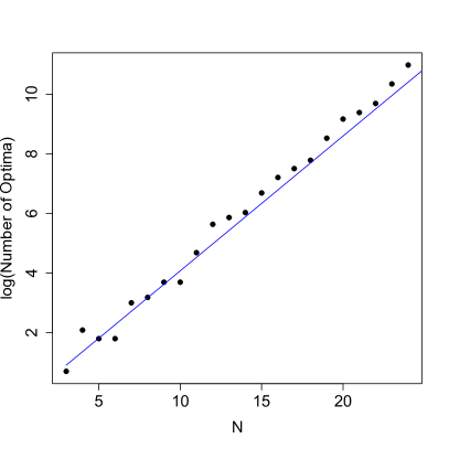
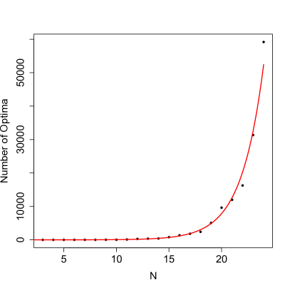
Figure 2: Number of optima in LABS problems as a function of the problem size $N$. Left Image: lin-log scale with a linear fit. Right image: linear scale with an exponential curve fit. Residual std. error: 0.2852, $R^{2}=0.9915$, p-value: $<$ 2.2e-16. The least squares regression line on the left image has equation: $y=0.47459\>x-0.5233$.

Since the global minimum always has some amount of degeneracy due to symmetry operation equivalencies, it is also of interest to compute the ratio of the total number of optima to the number of equivalent global optima for each $N$. This is shown in Fig. 3. From the plot it is clear that this ratio stays low for small $N$ but, as soon as $N$ nears $20$ the ratio takes off exponentially, although there are some fluctuations due to differences in symmetry. This behavior shows that the search for the global minimum remains exponentially harder for increasing $N$ despite the fact that there are several global minima.

Figure 3: The plot represents the ratio of the total number of optima to the number of global optima in LABS problems as a function of the problem size $N$. For $N$ moderately large, i.e., around $N=19$ and larger the number of optima that are global minima becomes a small fraction of the total number of optima in the energy landscape.

4.2 Average Degree

LABS LONs are weighted but it is still informative to plot their mean degree $\langle k\rangle$ by ignoring directions and weights and taking only the number of links into account. This gives Fig. 4 in which we see that the LONs are rather densely connected and $\langle k\rangle\propto N$.

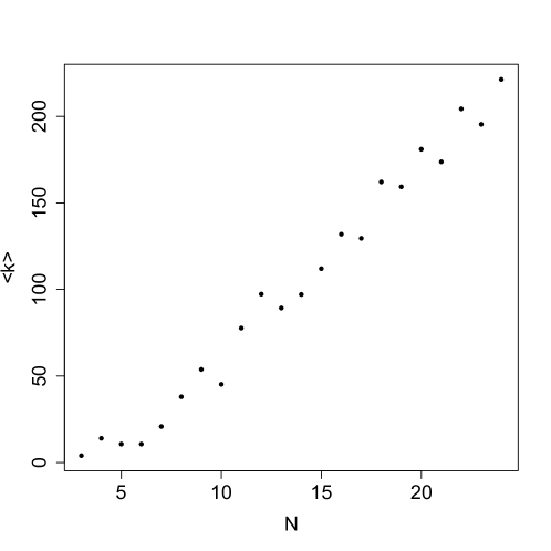
Figure 4: Average degree of the LABS LONS as a function of problem size $N$. Edge weights and direction are not taken into account for the computation, i.e. LONS are considered undirected and unweighted.

4.3 Average Strength

Node strength is informative because it is related to the probability of transition between energy basins. As such, it can provide useful information on the likely behavior of optimization methods that search the energy landscape. Figure 5 (left image) depicts the average strength $\langle w_{ii}\rangle$, i.e. the average weight of the transitions from a given optimum to itself. This value is a proxy for the average probability of remaining in a given energy basin once it has been reached. This empirical probability increases with increasing $N$ showing that a search that has reached a suboptimal minimum has an increasing tendency to remain in its basin.

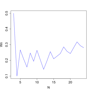
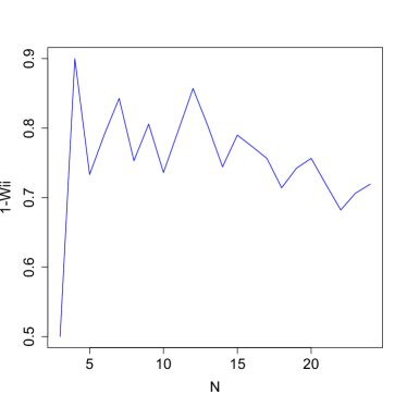
Figure 5: Average strength in LON graphs as a function of LON size $N$. Average link strength for self-loops $w_{ii}$ (left image) and outgoing links $1-w_{ii}$ (right image).

Since strength values are normalized to one, $w_{ij}=1-w_{ii}$ with $i\neq j$. Figure 5 (right image) shows the average strength of all the other outgoing links. Clearly, this view is the complementary of the previous one and it shows that outgoing, i.e., interbasin transitions become less probable with increasing $N$.

4.4 Degree Distribution Functions

The degree distribution function of a complex network may give some useful indication about the general structure of the latter, for example whether it belongs to a known class of distributions such as Poissonian, exponential, or power law. Here we deal with directed graphs and thus we have two distinct degree distributions: the incoming links distribution and the outgoing links distribution. We found that the LON degree distributions all show the same trend for different $N$ values except for very low $N$ for which the graphs have too few vertices. To illustrate the typical tendency, we show the in and out distributions for $N=17$ and $N=20$ in Fig. 6.

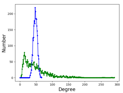
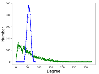
$N=17\hskip 147.95424ptN=20$

Figure 6: Degree distribution function for incoming (green curve) and outgoing (blue curve) links for $N=17$ (left plot) and $N=20$ (right plot).

The remarkable thing is that in and out distributions are very different. We did not try to fit any particular function to these empirical distributions; however, in a qualitative manner the outgoing links distribution (blue curve) appears to be close to Poissonian with a rather narrow peak and a smaller fluctuation around the mean. The incoming links distribution (green curve), on the other hand, is broader and has a much longer tail indicating that there is a non-negligible number of LON vertices with a large number of incoming links. This suggest that those nodes could play a role in dynamical processes on LONs. We shall see later that other measures tend to confirm this idea. For weighted networks strength distributions can also be computed but since they don’t bring new information in this case, we refrained from showing them to save space.

4.5 Basin Sizes

A useful by-product of the exhaustive LONs construction is that each admissible solution can be assigned to the basin of attraction of one of the optima in the LON. This allows us to define a basin’s size as being equal to the number of configurations that end up reaching the corresponding optimum using 1-bit flip and best improvement. Figure 7 shows the size of the global optimum basin as a function of $N$.

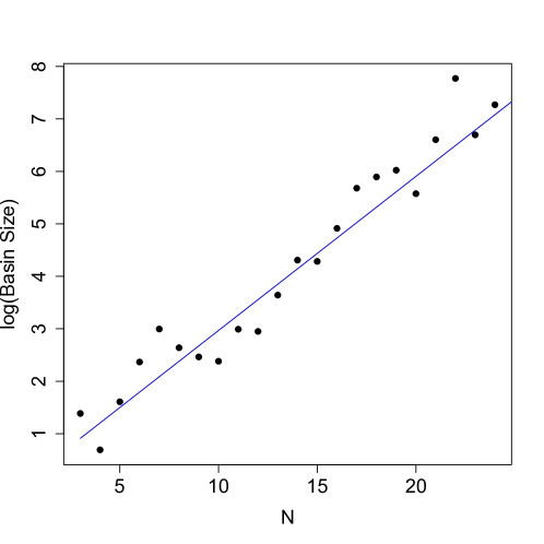
Figure 7: Basin Sizes of the global minimum as a function of $N$ on lin-log scale. A linear fit (blue line) gives a residual sd. err.: $0.4956$, $R^{2}=0.9419$, p-value: 4.895e-14. The equation of the least squares regression line is: $y=0.30765\>x-0.01078$.

First, let us observe again that all global energy minima are degenerate, i.e., there is always more than one global minimum with the same energy. For the figure, we simply plotted the size of one of the global minima chosen at random since all of them have the same or similar size. We observe that the size of the basin corresponding to a global optimum increases roughly exponentially with $N$. This would seem to suggest that it should be easier to find during an heuristic search. However, this effect is more than compensated for by the fact that the number of optima also increases exponentially with $N$ as shown in Fig. 2. In this highly rugged landscape, searches are thus likely to get stuck into one of the many good but not globally optimal minima. This phenomenon has previously been observed in other well known hard combinatorial optimization problems such as $NK$ landscapes and QAP [9, 19, 21, 22].

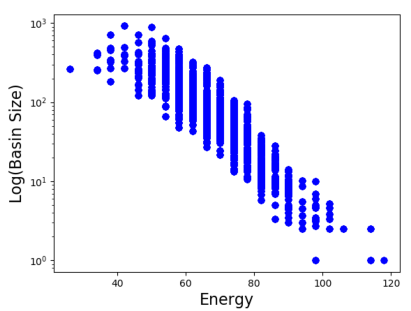
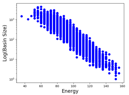
$N=20\hskip 147.95424ptN=24$

Figure 8: Logarithm of the basin of attraction size of the minima in the LON as a function of their energy. Energy values are sorted in increasing order. Left image: LON corresponding to $N=20$; right image: $N=24$.

Figures 8 show another aspect of the basin size distributions. The figures depict the basin size as a function of the corresponding minimum energy for $N=20$ (left image) and $N=24$ (right image). It clearly appears that there is an inverse relationship between the energy of a given minimum and the size of the corresponding basin. Thus, better minima have larger basin sizes. This is also in line with previous findings on this and similar problems [8, 22]. Again, since the largest basin(s) correspond to the best energy minima, it would appear that a search should be able to find one of them but actually this is not the case with $N$ large, because there is a myriad of other basins with only slightly worse energy and similar size in which the search might get trapped. The previous considerations tend to invalidate the “golf course” hypothesis put forward in [6] which states that the global minima for large $N$ are extremely rare and are isolated in the energy landscape. In fact, they are indeed rare but not isolated: in the picture that emerges examining their LONS, there is an exponentially increasing number of less good minima everywhere around that may attract the search. A similar conclusion has been reached by Ferreira et al. [8].

4.6 Shortest Paths

From the point of view of a search algorithm, a useful network measure is the average length of the shortest weighted path from the local optima to the global ones. The edge weights are important because their values are related to the transition probabilities between basins: an edge with a large weight means that the corresponding transition is more likely to occur and thus the edge’s length is proportional to the inverse of the weight in the path computation using the customary Dijkstra algorithm. The averages are shown in Fig. 9. Only the distances for the values of $N$ that have non-degenerate sets of minima are shown since for the others, i.e., for $N=3,4,6,10$ all the minima are global and thus the distance is zero. As well, we limit $N$ to $20$ since the exponential increase of the number of minima makes the many source-single destination shortest path algorithm to become too slow for larger $N$ values.

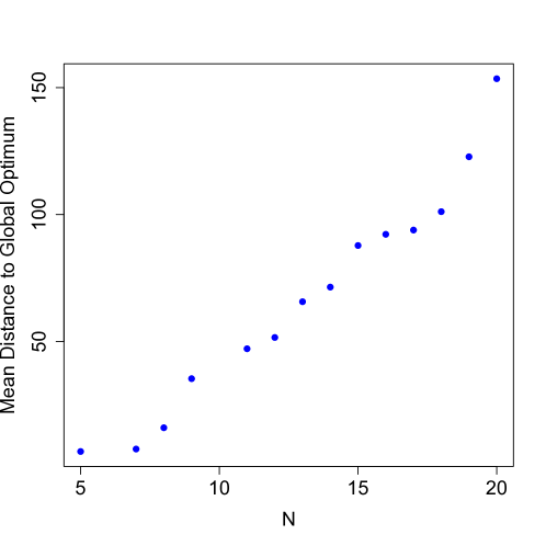
Figure 9: Average path lengths to a global optimum from all the other local optima for the LABS problems. Each point corresponds to a problem size $N$ for $N=5$ to $N=24$. The values $N=3,4,6,10$ are excluded because in this case all optima are global and thus the distance is zero.

The implication is that the length of the path increases with problem size; in other words it becomes harder and harder to reach a global optimum because the searcher must, on average, pass through an increasing number of local optima before reaching the global one which, in turn, is a consequence of the exponential increase of the number of optima. This can be alleviated to some extent by optimization heuristics such as simulated annealing which can in principle overcome energy barriers in the high temperature regime.

4.7 PageRank Centrality: Random Walks

The PageRank [23] algorithm provides a measure of the importance of a web page based on how much it is referenced by other important pages. The aim is to capture the prestige of each node in order to rank pages by importance and thus reduce the amount of information to process by an end user in a web search. The algorithm can be described as a random walk on the web considered as a directed graph. In a single step, the walker goes from a node $a$ to a neighboring node $b$ with a probability given by $1/k$, where $k$ is the number of outgoing links from vertex $a$. By definition of a random walk, after one step the probability distribution will be $\mathbf{p}_{1}=\mathbf{p}_{0}\;\mathbf{T}$ and from step $j$ to $j+1$ it changes as

$$\mathbf{p}_{j+1}=\mathbf{p}_{j}\;\mathbf{T}$$ (1)

Therefore, by iterating the previous equation from $j=0$ to $j=n-1$, the probability distribution ${\bf{p}}_{n}$ after $n$ steps is:

$$\mathbf{p}_{n}=\mathbf{p}_{0}\;\mathbf{T}{{}^{n}},$$

that is, it is given by the initial probability distribution vector times the $n$-th power of the transition matrix $\mathbf{T}$. In the long time limit, if some conditions are satisfied, the probability distribution may reach an invariant value given by $\mathbf{p}^{*}=(p_{1}^{*},\ldots,p_{N}^{*})_{\infty}$ with $p_{i}^{*}=lim_{n\rightarrow\infty}p_{i}(n)$. Substituting in eq. 1 gives

$$\mathbf{p}^{*}=\mathbf{p}^{*}\mathbf{T}$$

From this eigenvalue equation the equilibrium, or stationary, probability distribution is the left eigenvector of $\bf T$ with eigenvalue $1$ [24]. This equilibrium probability distribution of the above Markov chain gives the asymptotic frequency of visits to each node of the network. In PageRank there is a device that allows to get out of dead ends, i.e., when the walk reaches a node that does not have outgoing links, or to simulate starting a new browsing session. In this case, with some probability (around $0.2$) the walk jumps to a random node. This is not used here because LONS are strongly connected graphs by construction.

PageRank has already been used in the context of problem difficulty in [25]. Here we have applied PageRank to the LONS of the LABS problem. The results for $N=20$ and $N=24$ are given in Fig. 10, where nodes sorted by increasing energy are listed on the x-axis, and the corresponding PageRank centrality, i.e., the long-term frequency of visits of each node, is reported on the y-axis.

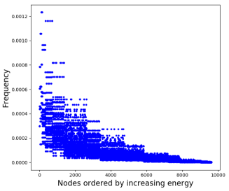
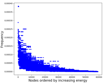
$N=20\hskip 156.49014ptN=24$

Figure 10: PageRank centrality of all minima versus their energies as measured by the frequency of visits during a random walk. Left picture: $N=20$; right picture: $N=24$. Energies increase to the right of the x-axis.

The important observation is that better optima, i.e. those close to the origin of the x-axis, are visited more often than less good ones. This is because the visit frequency depends on the incoming degree and, as better optima have larger basins, the corresponding LON nodes also have larger degree of the incoming links. Therefore, the result in terms of PageRank values is coherent with the picture that emerged previously when we analyzed the basins depths and sizes (see Fig. 8). Then, in principle, it would seem that the best optima should be easier to find than the worst ones. But this would be a wrong conclusion for two reasons. The first reason is that the “searcher” is just performing a random walk, in other words, it doesn’t make use of the energy information associated to each LON node. In this way, the walk can only reach the global optimum by chance. The second reason is that with increasing $N$ the number of optima increases exponentially (see Fig. 2). As a result, there is a very large number of suboptimal, but still very good, minima that will be visited during the random walk and only a handful among those are global optima.

5 Conclusions

In this contribution we have provided an up-to-date view of the structure of the energy landscape of the LABS problem which has important applications in communication engineering and in other fields, and is a typical representative of the $NP$-hard class for which no polynomial algorithm is known. Since enumerative algorithms cannot be used for large $N$ as they take too long to terminate, metaheuristics searches are often used. These searches benefit the most from a better knowledge of the underlying energy landscape since they work by sampling the latter in clever ways. To study the landscape features of interest we have made use of the local optima network methodology by systematically extracting the problem optima graphs for $N$ values up to $N=24$. Several metrics were used to characterize the networks: number and type of optima, optima basins structure, degree and strength distributions, shortests paths to the global optima, and random walk-based centrality of optima. Taken together, these metrics provide a quantitative and coherent explanation for the difficulty of the LABS problem and give information about the energy landscape that can be exploited for this problem as well as a number of other problems having a similar configuration space structure. The methodology used here and the results presented above are also potentially useful for the investigation of the energy landscape of spin glasses which, in spite of being disordered systems by definition, have a number of similarities with the present problem, p-spin systems in particular. Future work is planned in this direction.

Acknowledgements.

I am grateful to Sébastien Vérel for useful discussions and for producing the local optima graphs.

References

- [1] M. Golay. The merit factor of long low autocorrelation binary sequences (corresp.). IEEE Transactions on Information Theory, 28(3):543–549, 1982.
- [2] E. Marinari, G. Parisi, and F. Ritort. Replica field theory for deterministic models: I. binary sequences with low autocorrelation. Journal of Physics A: Mathematical and General, 27(23):7615, 1994.
- [3] J. Jedwab. A survey of the merit factor problem for binary sequences. In International Conference on Sequences and Their Applications, pages 30–55. Springer, 2004.
- [4] T. Packebusch and S. Mertens. Low autocorrelation binary sequences. Journal of Physics A: Mathematical and Theoretical, 49(16):165001, 2016.
- [5] B. Bošković, F. Brglez, and J. Brest. Low-autocorrelation binary sequences: On improved merit factors and runtime predictions to achieve them. Applied Soft Computing, 56:262–285, 2017.
- [6] J. Bernasconi. Low autocorrelation binary sequences: statistical mechanics and configuration space analysis. Journal de Physique, 48(4):559–567, 1987.
- [7] J.-P. Bouchaud and M. Mézard. Self induced quenched disorder: a model for the glass transition. Journal de Physique I, 4(8):1109–1114, 1994.
- [8] F. F. Ferreira, J. Fontanari, and P. F. Stadler. Landscape statistics of the low-autocorrelation binary string problem. Journal of Physics A: Mathematical and General, 33(48):8635, 2000.
- [9] M. Tomassini, S. Verel, and G. Ochoa. Complex-network analysis of combinatorial spaces: The NK landscape case. Phys. Rev. E, 78(6):066114, 2008.
- [10] F. Daolio, M. Tomassini, S. Vérel, and G. Ochoa. Communities of minima in local optima networks of combinatorial spaces. Physica A Statistical Mechanics and its Applications, 390:1684–1694, 2011.
- [11] C.M. Reidys and P.F. Stadler. Combinatorial landscapes. SIAM review, 44(1):3–54, 2002.
- [12] S. Verel, G. Ochoa, and M. Tomassini. Local optima networks of NK landscapes with neutrality. IEEE Transactions on Evolutionary Computation, 15(6):783–797, 2011.
- [13] S. Verel, F. Daolio, G. Ochoa, and M. Tomassini. Local optima networks with escape edges. In Proceedings of the International Conference on Artificial Evolution, EA-2011, volume 7401 of Lecture Notes in Computer Science, pages 49–60. Springer, 2012.
- [14] S. L. Thomson, G. Ochoa, and S. Verel. Clarifying the difference in local optima network sampling algorithms. In European Conference on Evolutionary Computation in Combinatorial Optimization (Part of EvoStar), pages 163–178. Springer, 2019.
- [15] F. H. Stillinger. Energy Landscapes, Inherent Structures, and Condensed-Matter Phenomena. Princeton University Press, Princeton, 2016.
- [16] M. Newman. Networks. Oxford university press, 2018.
- [17] A.-L. Barabási. Network science. Cambridge university press, 2016.
- [18] S. A. Kauffman. The Origins of Order. Oxford University Press, New York, 1993.
- [19] M. Tayarani and A. Prügel-Bennett. Quadratic assignment problem: a landscape analysis. Evolutionary Intelligence, 8(4):165–184, 2015.
- [20] F. Ferreira and J. F Fontanari. Probabilistic analysis of the number partitioning problem. Journal of Physics A: Mathematical and General, 31(15):3417, 1998.
- [21] F. Daolio, S. Verel, G. Ochoa, and M. Tomassini. Local Optima Networks of the Quadratic Assignment Problem. In Evolutionary Computation (CEC), 2010 IEEE Congress on, pages 1–8. IEEE, 2010.
- [22] L. Hernando, A. Mendiburu, and J. A. Lozano. Anatomy of the attraction basins: Breaking with the intuition. Evolutionary Computation, 27(3):435–466, 2019.
- [23] S. Brin and L. Page. The anatomy of a large-scale hypertextual web search engine. Computer networks and ISDN systems, 30(1-7):107–117, 1998.
- [24] N. Masuda, M. A. Porter, and R. Lambiotte. Random walks and diffusion in networks. Physics Reports, 716:1–58, 2017.
- [25] S. Herrmann, G. Ochoa, and F. Rothlauf. Pagerank centrality for performance prediction: the impact of the local optima network model. Journal of Heuristics, 24(3):243–264, 2018.