A New Diffusive Representation for Fractional Derivatives and its Application

Abstract

Diffusive representations of fractional derivatives have proven to be useful tools in the construction of fast and memory efficient numerical methods for solving fractional differential equations. A common challenge in many of the known variants of this approach is that they require the numerical approximation of some integrals over an unbounded integral whose integrand decays rather slowly which implies that their numerical handling is difficult and costly. We present a novel variant of such a diffusive representation. This form also requires the numerical approximation of an integral over an unbounded domain, but the integrand decays much faster. This allows to use well established quadrature rules with much better convergence properties.

1 Introduction and Statement of the Problem

1.1 Classical Discretizations in Fractional Calculus

The efficient numerical solution of initial value problems with fractional differential equations like, e.g.,

$$D^{\alpha}_{a}y(t)=f(t,y(t)),\qquad y(a)=y_{0},$$ (1)

is a significant computational challenge due to, among other reasons, the non-locality of fractional differential operators. In our formulation (1), $D^{\alpha}_{a}$ denotes the standard Caputo differential operator of order $\alpha$ with starting point $a\in\mathbb{R}$ [6, Chapter 3], and we assume here and throughout some other parts of this paper that $0<\alpha<1$ (although we explicitly point out that the generalization of our findings to the case that $\alpha$ is a noninteger number greater than $1$ is a relatively straightforward matter).

When dealing with the problem (1), one usually introduces a discretization of the interval $[a,a+T]$, say, on which the solution is sought by defining some grid points $a=t_{0}<t_{1}<t_{2}<\cdots<t_{N}=a+T$. For each grid point $t_{j}$, $j=1,2,\ldots,N$, typical numerical methods then introduce an approximation formula for a discretization of $D_{a}^{\alpha}y(t_{j})$ based on function values of $y$ at the grid points, replace the exact fractional derivative in eq. (1) by this approximation, discard the approximation error and solve the resulting algebraic equation to obtain an approximation for $y(t_{j})$. In their standard forms, classical methods like fractional linear multistep methods [19, 20] or the Adams method [8, 9] require $O(j)$ operations to compute the required approximation at the $j$-th grid point, thus leading to an $O(N^{2})$ complexity for the overall calculation of the approximate solution at all $N$ grid points. Moreover, the construction of the algorithms requires the entire history of the process to be in the active memory at any time, thus leading to an $O(N)$ memory requirement. This may be prohibitive in situations like, e.g., the simulation of the mechanical behaviour of viscoelastic materials via some finite element code where a very large number of such differential equations needs to be solved simultaneously [17].

Numerous modifications of these basic algorithms have been proposed to resolve these issues. Specifically (see, e.g., [11, Section 3]), one may use FFT techniques to evaluate the sums that arise in the formulas [13, 14, 15], thus reducing the overall computational complexity to $O(N\log^{2}N)$; however, this approach does not improve the memory requirements. Alternatively, nested mesh techniques [10, 12] can be employed; this typically reduces the computational complexity to $O(N\log N)$, and some of these methods are also able to cut down the active memory requirements to $O(\log N)$.

1.2 Diffusive Representations in Discretized Fractional Calculus

From the properties recalled above, it becomes clear that none of the schemes mentioned so far allows to reach the level known for traditional algorithms for first order initial value problems that, due to their differential operators being local, have an $O(N)$ complexity and an $O(1)$ memory requirement. However, it is possible to achieve these perfomance features by using methods based on diffusive representations for the fractional derivatives [23]. Typically, such representations take the form

$$D_{a}^{\alpha}y(t)=\int_{0}^{\infty}\phi(w,t)\mathrm{d}w$$ (2)

where, for a fixed value of $w$, the function $\phi(w,\cdot)$ is characterized as the solution to an initial value problem for a first order differential equation the formulation of which contains the function $y$ whose fractional derivative is to be computed. In the presently available literature, many different special cases of this representation are known, e.g. the version of Yuan and Agrawal [28] (originally proposed in that paper for $0<\alpha<1$ and extended to $1<\alpha<2$ in [27] and to general positive noninteger values of $\alpha$ in [5]; see also [24] for further properties of this method) where the associated initial value problem reads

$$\frac{\partial\phi^{\mathrm{YA}}}{\partial t}(w,t)\!=\!-w^{2}\phi^{\mathrm{YA}}\!(w,t)\!+\!(\!-1\!)^{\lfloor\!\alpha\!\rfloor}\frac{2\sin\pi\alpha}{\pi}w^{2\alpha-2\lceil\!\alpha\!\rceil+1}y^{(\lceil\!\alpha\!\rceil)}(t),\,\,\phi^{\mathrm{YA}}\!(w,a)=0,$$ (3a)

such that the function $$\phi^{\mathrm{YA}}$$ has the form

$$\phi^{\mathrm{YA}}(w,t)=(-1)^{\lfloor\alpha\rfloor}\frac{2\sin\pi\alpha}{\pi}w^{2\alpha-2\lceil\alpha\rceil+1}\int_{a}^{t}y^{(\lceil\alpha\rceil)}(\tau)\exp(-(x-\tau)w^{2})\mathrm{d}\tau.$$ (3b)

An alternative has been proposed by Chatterjee [3] (see also [25]) using the initial value problem

$$\frac{\partial\phi^{\mathrm{C}}}{\partial t}(w,t)\!=\!-w^{1/(\alpha-\lceil\!\alpha\!\rceil+1)}\phi^{\mathrm{C}}\!(w,t)+(\!-1\!)^{\lfloor\!\alpha\!\rfloor}\frac{\sin\pi\alpha}{\pi(\alpha-\lceil\!\alpha\!\rceil+1)}y^{(\lceil\!\alpha\!\rceil)}(t),\quad\phi^{\mathrm{C}}\!(w,a)=0,$$ (4a)

such that the function $$\phi^{\mathrm{C}}$$ has the form

$$\phi^{\mathrm{C}}(w,t)=\frac{(-1)^{\lfloor\alpha\rfloor}\sin\pi\alpha}{\pi(\alpha-\lceil\alpha\rceil+1)}\int_{a}^{t}y^{(\lceil\alpha\rceil)}(\tau)\exp\left(-(t-\tau)w^{1/(\alpha-\lceil\alpha\rceil+1)}\right)\mathrm{d}\tau.$$ (4b)

In either case (or in the case of the many variants thereof that have been proposed; cf., e.g., [1, 2, 18, 22, 29]), the numerical calculation of $D^{\alpha}_{a}y(t_{j})$ requires

1. a quadrature formula

   $$\sum_{k=1}^{K}\lambda_{k}\phi(w_{k},t_{j})\approx\int_{0}^{\infty}\phi(w,t_{j})\mathrm{d}w=D_{a}^{\alpha}y(t_{j})$$ (5)

   with nodes $w_{1},w_{2},\ldots,w_{K}\in[0,\infty)$ and weights $\lambda_{1},\lambda_{2},\ldots,\lambda_{K}\in\mathbb{R}$ for numerically evaluating the integral in eq. (2)

2. a standard numerical solver for the associated differential equation (e.g., a linear multistep method) to approximately compute, for each $k\in\{1,2,\ldots,K\}$, the values $\phi(w_{k},t_{j})$ required to evaluate the formula (5).

Evidently, the run time and the memory requirements of the operation in step 1 do not depend on $j$. Also, one can perform step 2 in an amount of time that is independent of $j$. Furthermore, if an $\ell$-step method is used in step 2, one needs to have (approximate) information about $y(t_{j-1}),y(t_{j-2}),\ldots y(t_{j-\ell})$ which has to be kept in the active memory—but the amount of storage space required for this purpose is also independent of $j$.

In summary, approaches of this type require $O(1)$ arithmetic operations per time step, i.e. we have a computational cost of $O(N)$ for all $N$ time steps combined, and the required amount of memory is $O(1)$ as desired. A further pleasant property of these methods is that they impose no restrictions at all on the choice of the grid points $t_{j}$ whereas this can not always be achieved with the other approaches. Thus, from a theoretical point of view, algorithms of this form are very attractive. In practice, however, the implied constants in the $O$-terms may be very large. This is due to the following observation [6, Theorems 3.20(b) and 3.21(b)]:

Proposition 1.1.

Let $t\in[a,a+T]$ be fixed. Then, for $w\to\infty$, we have

$$\phi^{\mathrm{YA}}(w,t)=c^{\mathrm{YA}}w^{q_{\mathrm{YA}}}(1+o(1))\quad\mbox{ with }\quad q_{\mathrm{YA}}=2\alpha-2\lceil\alpha\rceil-1\in(-3,-1)$$

and

$$\phi^{\mathrm{C}}(w,t)=c^{\mathrm{C}}w^{q_{\mathrm{C}}}(1+o(1))\quad\mbox{ with }\quad q_{\mathrm{C}}=-\frac{1}{\alpha-\lceil\alpha\rceil+1}<-1$$

where $c^{\mathrm{C}}$ and $c^{\mathrm{YA}}$ are some constants independent of $w$ (that may, however, depend on $t$, $a$, $\alpha$ and $y$).

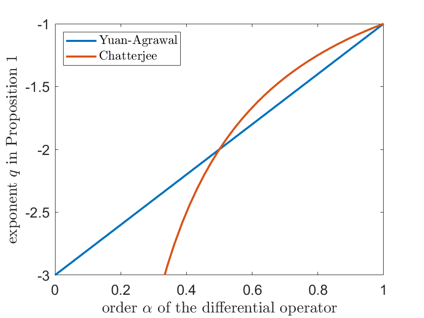
Figure 1: Behaviour of the exponents $q_{\mathrm{YA}}$ (blue) and $q_{\mathrm{C}}$ (orange) as introduced in Proposition 1.1 vs. the order $\alpha$ of the differential operator

From Proposition 1.1 we can see that the integrands in eq. (2) decay to zero in an algebraic manner as $w\to\infty$. Figure 1 shows the behaviour of the exponents $q_{\mathrm{YA}}$ and $q_{\mathrm{C}}$ as they depend on $\alpha$. It can be seen that the exponents are less than $-1$ for all $\alpha\in(0,1)$. This suffices to assert that the integrals $\int_{0}^{\infty}\phi(w,t)\mathrm{d}w$ are convergent. On the other hand, step 1 of the algorithm outlined above requires to numerically approximate this integral, and to this end, classical results from approximation theory [21] imply that such an algebraic decay does not admit a very fast convergence of such numerical methods. Indeed, as the constant $q^{\mathrm{C}}$ is slightly larger than $q^{YA}$ for $\alpha\geq 1/2$ and (significantly) smaller for $\alpha<1/2$, one may state that overall Chatterjee’s method has more preferable properties from this point of view (although its properties are still far from good enough). To the best of the author’s knowledge, this is a feature shared by very many algorithms based on this type of approach. Therefore, one needs a relatively large number $K$ of quadrature nodes in eq. (5) to obtain an approximation with an acceptable accuracy (with the approaches known so far, a common choice for $K$ is in the range between 200 and 500, cf. [1, 17]). This number $K$ clearly has a strong influence on the constants implied in the $O$-term for the computational complexity estimate. The main goal of this paper thus is to develop a method that is also based on the same fundamental idea but that leads to a function $\phi(w,t)$ which exhibits an exponential decay for large $w$. This behaviour is much more pleasant from an approximation theoretic point of view because it allows to use well understood and rapidly convergent classical techniques like Gauss-Laguerre quadrature formulas. The hope behind this idea is that the improved convergence behaviour will admit to use quadrature formulas as in eq. (5) with a significantly smaller number $K$ of nodes, so that the resulting algorithms can produce results with a comparable accuracy as the known methods in a much shorter amount of time (that is still proportional to $N$ but with a significantly smaller implied constant).

2 The New Diffusive Representation and its Properties

Our main idea is based on the following result.

Theorem 2.1.

For given values $a\in\mathbb{R}$, $T>0$ and $\alpha\in\mathbb{R}_{+}\setminus\mathbb{N}$ and a given function $y\in C^{\lceil\alpha\rceil}[a,a+T]$, let

$$q_{\mathrm{D}}=\alpha-\lceil\alpha\rceil+1$$ (6)

and

$$\phi^{\mathrm{D}}(w,t)=(-1)^{\lfloor\alpha\rfloor}\frac{\sin\alpha\pi}{\pi}\mathrm{e}^{wq_{\mathrm{D}}}\int_{a}^{t}y^{(\lceil\alpha\rceil)}(\tau)\exp\left(-(t-\tau)\mathrm{e}^{w}\right)\mathrm{d}\tau$$ (7)

for all $w\in\mathbb{R}$ and $t\in[a,a+T]$. Then, we have the following properties:

1. The value $q_{\mathrm{D}}$ satisfies $0<q_{\mathrm{D}}<1$.

2. For any $w\in\mathbb{R}$, the function $\phi^{\mathrm{D}}(w,\cdot)$ solves the initial value problem

   $$\frac{\partial\phi^{\mathrm{D}}}{\partial t}(w,t)=-\mathrm{e}^{w}\phi^{\mathrm{D}}(w,t)+(-1)^{\lfloor\alpha\rfloor}\frac{\sin\alpha\pi}{\pi}\mathrm{e}^{wq_{\mathrm{D}}}y^{(\lceil\alpha\rceil)}(t),\quad\phi^{\mathrm{D}}(w,a)=0$$ (8)

   for $t\in[a,a+T]$.

3. For any $t\in[a,a+T]$,

   $$D_{a}^{\alpha}y(t)=\int_{-\infty}^{\infty}\phi^{\mathrm{D}}(w,t)\mathrm{d}w.$$ (9)

4. For any $t\in[a,a+T]$, we have $\phi^{\mathrm{D}}(\cdot,t)\in C^{\infty}(\mathbb{R})$.

5. For any $t\in[a,a+T]$,

   $$\phi^{\mathrm{D}}(w,t)=O(\mathrm{e}^{w(q_{\mathrm{D}}-1)})\quad\mbox{ as }w\to\infty$$ (10)

   and

   $$\phi^{\mathrm{D}}(w,t)=O(\mathrm{e}^{wq_{\mathrm{D}}})\quad\mbox{ as }w\to-\infty.$$ (11)

So, part (b) of Theorem 2.1 asserts that our function $\phi^{\mathrm{D}}$ solves an initial value problem of the same type as the previously considered functions, cf. (3a) or (4a). Moreover, according to part (c), by integrating this function with respect to $w$ we obtain the fractional derivative of the given function $y$, which is in analogy with the corresponding equation (2) for the known approaches mentioned above. Note that there is a marginal difference between eqs. (2) and (9) in the sense that the latter involves an integration over the entire real line whereas the former requires to integrate over the positive half line only, but from the point of view of approximation (or quadrature) theory this does not introduce any substantial problems. (The index $\mathrm{D}$ in $\phi^{\mathrm{D}}$ and $q_{\mathrm{D}}$ can be interpreted to stand for “doubly infinite integration range”.) Thus, in these respects the new model behaves in very much the same way as the known ones. The significant difference between the known approach and the new one is evident from part (e) of the Theorem: It asserts (in view of the property of $q_{\mathrm{D}}$ shown in part (a)) that the integrand exhibits the desired exponential decay as $w\to\pm\infty$, thus allowing, in combination with the smoothness result of part (d), a much more efficient numerical integration.

Proof.

Part (a) is an immediate consequence of the definition of $q_{\mathrm{D}}$ given in eq. (6).

For part (b), we first note that the integrand in eq. (7) is continuous by assumption. Hence, the integral is zero for $t=a$ which implies that the initial condition given in eq. (8) is correct. Also, a standard differentiation of the integral in the definition (7) with respect to the parameter $t$ yields the differential equation.

To prove (c), we recall from [6, Proof of Theorem 3.18] that

$$D_{a}^{\alpha}y(t)=(-1)^{\lfloor\alpha\rfloor}\frac{\sin\alpha\pi}{\pi}\int_{a}^{t}\int_{0}^{\infty}\frac{\mathrm{e}^{-z}}{z}\left(\frac{z}{x-\tau}\right)^{q_{\mathrm{D}}}y^{(\lceil\alpha\rceil)}(\tau)\mathrm{d}z\,\mathrm{d}\tau.$$

The substitution $z=(x-\tau)\mathrm{e}^{w}$, combined with an interchange of the two integrations (that is admissible in view of Fubini’s theorem), then leads to the desired result.

Statement (d) directly follows from the definition (7) of the function $\phi^{\mathrm{D}}$.

Finally, we show that the estimates of (e) are true. To this end, let us first discuss what happens for $w\to+\infty$. Here, we can see that

$$\phi^{\mathrm{D}}(w,t)=(-1)^{\lfloor\alpha\rfloor}\frac{\sin\alpha\pi}{\pi}(I_{1}+I_{2})$$

where

$$|I_{1}| =\left|\mathrm{e}^{wq_{\mathrm{D}}}\int_{t-w\exp(-w)}^{t}y^{(\lceil\alpha\rceil)}(\tau)\exp\left(-(t-\tau)\mathrm{e}^{w}\right)\mathrm{d}\tau\right|$$

$$\leq\|y^{(\lceil\alpha\rceil)}\|_{L_{\infty}[a,a+T]}\mathrm{e}^{wq_{\mathrm{D}}}\left|\int_{t-w\exp(-w)}^{t}\exp\left(-(t-\tau)\mathrm{e}^{w}\right)\mathrm{d}\tau\right|$$

$$\leq\|y^{(\lceil\alpha\rceil)}\|_{L_{\infty}[a,a+T]}\mathrm{e}^{wq_{\mathrm{D}}}\mathrm{e}^{-w}\left[1-\mathrm{e}^{-w}\right]<\|y^{(\lceil\alpha\rceil)}\|_{L_{\infty}[a,a+T]}\mathrm{e}^{w(q_{\mathrm{D}}-1)}$$

and

$$|I_{2}| =\left|\mathrm{e}^{wq_{\mathrm{D}}}\int_{a}^{t-w\exp(-w)}y^{(\lceil\alpha\rceil)}(\tau)\exp\left(-(t-\tau)\mathrm{e}^{w}\right)\mathrm{d}\tau\right|$$

$$\leq\mathrm{e}^{wq_{\mathrm{D}}}\max_{\tau\in[a,t-w\exp(-w)]}\exp\left(-(t-\tau)\mathrm{e}^{w}\right)\int_{a}^{t-w\exp(-w)}|y^{(\lceil\alpha\rceil)}(\tau)|\mathrm{d}\tau$$

$$\leq\mathrm{e}^{wq_{\mathrm{D}}}\mathrm{e}^{-w}\int_{a}^{a+T}|y^{(\lceil\alpha\rceil)}(\tau)|\mathrm{d}\tau=\mathrm{e}^{w(q_{\mathrm{D}}-1)}\int_{a}^{a+T}|y^{(\lceil\alpha\rceil)}(\tau)|\mathrm{d}\tau$$

which shows the desired result (10) in this case; in particular, the upper bound decays exponentially for $w\to\infty$ because $q_{\mathrm{D}}<1$. Regarding the behaviour for $w\to-\infty$, we start from the representation (7) and apply a partial integration. This yields, taking into consideration that $t\geq a$, that

$$|\phi^{\mathrm{D}}(w,t)| =\frac{|\sin\alpha\pi|}{\pi}\mathrm{e}^{wq_{\mathrm{D}}}\Big{|}\exp\left(-(x-\tau)\mathrm{e}^{w}\right)y^{(\lceil\alpha\rceil-1)}(\tau){\big{|}}_{\tau=a}^{\tau=t}$$

$$\qquad\qquad\qquad\qquad-\mathrm{e}^{w}\int_{a}^{t}\exp\left(-(t-\tau)\mathrm{e}^{w}\right)y^{(\lceil\alpha\rceil-1)}(\tau)\mathrm{d}\tau\Big{|}$$

$$\leq\frac{|\sin\alpha\pi|}{\pi}\mathrm{e}^{wq_{\mathrm{D}}}\left|y^{(\lceil\alpha\rceil-1)}(t)-y^{(\lceil\alpha\rceil-1)}(a)\exp\left(-(t-a)\mathrm{e}^{w}\right)\right|$$

$$\phantom{\leq}\quad{}+\frac{|\sin\alpha\pi|}{\pi}\mathrm{e}^{wq_{\mathrm{D}}}\|y^{(\lceil\alpha\rceil-1)}\|_{L_{\infty}[a,a+T]}\left|\mathrm{e}^{w}\int_{a}^{t}\exp\left(-(t-\tau)\mathrm{e}^{w}\right)\mathrm{d}\tau\right|$$

$$\leq\frac{|\sin\alpha\pi|}{\pi}\|y^{(\lceil\alpha\rceil-1)}\|_{L_{\infty}[a,a+T]}\mathrm{e}^{wq_{\mathrm{D}}}\left(2+1-\exp\left(-(t-a)\mathrm{e}^{w}\right)\right)$$

$$\leq 3\frac{|\sin\alpha\pi|}{\pi}\|y^{(\lceil\alpha\rceil-1)}\|_{L_{\infty}[a,a+T]}\mathrm{e}^{wq_{\mathrm{D}}},$$

thus proving the relation (11) and demonstrating, in view of $q_{\mathrm{D}}>0$, that $\phi^{\mathrm{D}}(w,t)$ decays to zero exponentially as $w\to-\infty$. ∎

3 The Complete Numerical Method

Based on Theorem 2.1—in particular, using the properties shown in parts (d) and (e)—we thus proceed as follows to obtain the required approximation of $D_{a}^{\alpha}y(t_{j})$, $j=1,2,\ldots,N$. Splitting up the integral from eq. (9) into the integrals over the negative and over the positive half line, respectively, and introducing some obvious substitutions, we notice that

$$\int_{-\infty}^{\infty}\phi^{\mathrm{D}}(w,t)\mathrm{d}w =\frac{1}{q_{\mathrm{D}}}\int_{0}^{\infty}\mathrm{e}^{-u}\mathrm{e}^{u}\phi^{\mathrm{D}}(-u/q_{\mathrm{D}},t)\mathrm{d}u$$

$$\phantom{=}\quad{}+\frac{1}{1-q_{\mathrm{D}}}\int_{0}^{\infty}\mathrm{e}^{-u}\mathrm{e}^{u}\phi^{\mathrm{D}}(u/(1-q_{\mathrm{D}}),t)\mathrm{d}u.$$

Therefore, using

$$\hat{\phi}^{\mathrm{D}}(u,t):=\mathrm{e}^{u}\left(\frac{1}{q_{\mathrm{D}}}\phi^{\mathrm{D}}(-u/q_{\mathrm{D}},t)+\frac{1}{1-q_{\mathrm{D}}}\phi^{\mathrm{D}}(u/(1-q_{\mathrm{D}}),t)\right),$$ (12)

we find that

$$D^{\alpha}_{a}y(t)=\int_{-\infty}^{\infty}\phi^{\mathrm{D}}(w,t)\mathrm{d}w=\int_{0}^{\infty}\mathrm{e}^{-u}\hat{\phi}^{\mathrm{D}}(u,t)\mathrm{d}u\approx Q^{\mathrm{GLa}}_{K}[\hat{\phi}^{\mathrm{D}}(\cdot,t)]$$ (13)

where

$$Q^{\mathrm{GLa}}_{K}[f]=\sum_{k=1}^{K}a^{\mathrm{GLa}}_{k}f(x^{\mathrm{GLa}}_{k})$$

is the $K$-point Gauss-Laguerre quadrature formula, i.e. the Gaussian quadrature formula for the weight function $\mathrm{e}^{-u}$ on the interval $[0,\infty)$ [4, Sections 3.6 and 3.7]. For the sake of simplicity, we have chosen to omit from our notation for the nodes $x^{\mathrm{GLa}}_{k}$ and the weights $a^{\mathrm{GLa}}_{k}$ of the Gauss-Laguerre quadrature formula the fact that these quantities depend on the total number $K$ of quadrature nodes. From [4, p. 227] and our Theorem 2.1 above, we can immediately conclude the following result:

Theorem 3.1.

Under the assumptions of Theorem 2.1, we have

$$\lim_{K\to\infty}Q^{\mathrm{GLa}}_{K}[\hat{\phi}^{\mathrm{D}}(\cdot,t)]=D^{\alpha}_{a}y(t)$$

for all $t\in[a,a+T]$.

For a given number $K$ of quadrature points, it is known that the nodes $x^{\mathrm{GLa}}_{k}$, $k=1,2,\ldots,K$, are the zeros of the Laguerre polynomial $L_{K}$ of order $K$, and the associated weights are given by

$$a^{\mathrm{GLa}}_{k}=\frac{x^{\mathrm{GLa}}_{k}}{[L_{K+1}(x_{k})]^{2}},$$

cf., e.g., [4, p. 223]. (In our definition of the Laguerre polynomials, the normalization is such that $\int_{0}^{\infty}\mathrm{e}^{-x}(L_{K}(x))^{2}\mathrm{d}x=1$.) From [26, eqs. (6.31.7), (6.31.11) and (6.31.12)] we know that, at least for $K\geq 3$,

$$\frac{2.89}{2K+1}<x^{\mathrm{GLa}}_{1}<\frac{3}{2K}\quad\mbox{ and }\quad 2K<x^{\mathrm{GLa}}_{K}<4K+3.$$

We are now in a position to describe the method for the numerical computation of $D^{\alpha}_{a}y(t_{j})$, $j=1,2,\ldots,N$, that we propose. In this algorithm, the symbol $\phi_{k}$ is used to denote the approximate value of $\phi^{\mathrm{D}}(x^{\mathrm{GLa}}_{k},t_{j})$ for the current time step. i.e. for the currently considered value of $j$. Steps 1 and 2 here are merely preparatory in nature; the core of the algorithm is step 3.

Given the initial point $a$, the order $\alpha$, the grid points $t_{j}$, $j=1,2,\ldots,N$ and the number $K\in\mathbb{N}$ of quadrature nodes,

1. Set $q_{\mathrm{D}}\mapsfrom\alpha-\lceil\alpha\rceil+1$.

2. For $k=1,2,\ldots,K$:

   1. compute the Gauss-Laguerre nodes $x^{\mathrm{GLa}}_{k}$ and the associated weights $a^{\mathrm{GLa}}_{k}$,

   2. define the auxiliary quantities $w_{k}\mapsfrom-x^{\mathrm{GLa}}_{k}/q_{\mathrm{D}}$ and $\tilde{w}_{k}\mapsfrom x^{\mathrm{GLa}}_{k}/(1-q_{\mathrm{D}})$,

   3. set $\phi_{k}\mapsfrom 0$ and $\tilde{\phi}_{k}\mapsfrom 0$ (to represent the initial condition of the differential equation (8) for $t=t_{0}=a$).

3. For $j=1,2,\ldots,N$:

   1. Set $h\mapsfrom t_{j}-t_{j-1}$.

   2. For $k=1,2,\ldots,K$:

      1. update the value $\phi_{k}$ by means of solving the associated differential equation (8) with, e.g., the backward Euler method, viz.

         $$\phi_{k}\mapsfrom\frac{1}{1+h\mathrm{e}^{w_{k}}}\left(\phi_{k}+h(-1)^{\lfloor\alpha\rfloor}\frac{\sin\alpha\pi}{\pi}\mathrm{e}^{w_{k}q_{\mathrm{D}}}y^{(\lceil\alpha\rceil)}(t_{j})\right)$$ (14a)

         (note that the index $k$ used here is not the time index);

      2. similarly, update the value $\tilde{\phi}_{k}$ by

         $$\tilde{\phi}_{k}\mapsfrom\frac{1}{1+h\mathrm{e}^{\tilde{w}_{k}}}\left(\tilde{\phi}_{k}+h(-1)^{\lfloor\alpha\rfloor}\frac{\sin\alpha\pi}{\pi}\mathrm{e}^{\tilde{w}_{k}q_{\mathrm{D}}}y^{(\lceil\alpha\rceil)}(t_{j})\right).$$ (14b)

   3. Compute the desired approximate value for $D^{\alpha}_{a}y(t_{j})$ using the formula

      $$D^{\alpha}_{a}y(t_{j})=\sum_{k=1}^{K}a^{\mathrm{GLa}}_{k}\exp(x^{\mathrm{GLa}}_{k})\left(\frac{1}{q_{\mathrm{D}}}\phi_{k}+\frac{1}{1-q_{\mathrm{D}}}\tilde{\phi}_{k}\right).$$

The main goal of this paper is to develop a diffusive representation that can be numerically handled in a more efficient way than traditional formuals. Therefore, our work concentrates on the aspects related to the integral, i.e. on the properties of the integrand and on the associated numerical quadrature. The solution of the differential equation is not in the focus of our work; we only use some very simple (but nevertheless reasonable) methods here. Our specific choice is based on the observation that the magnitude of the constant factor with which the unkonwn function $\phi(w,\cdot)$ on the right-hand side of (8) is multiplied is such that an A-stable method should be used [16]. Therefore, as the simplest possible choice among these methods, we have suggested the backward Euler method in our description given above. Alternatively, one could, e.g., use the trapezoidal method which is also A-stable. This would mean that the formulas given in eqs. (14a) and (14b) would have to be replaced by

$$\phi_{k} \mapsfrom\frac{1}{1+h\mathrm{e}^{w_{k}}/2}\Bigg{(}\left(1-\frac{h}{2}\mathrm{e}^{w_{k}}\right)\phi_{k}$$ (15a)

$$\phantom{mapsfrom}{}\qquad\qquad+\frac{h}{2}(-1)^{\lfloor\alpha\rfloor}\frac{\sin\alpha\pi}{\pi}\mathrm{e}^{w_{k}q_{\mathrm{D}}}(y^{(\lceil\alpha\rceil)}(t_{j})+y^{(\lceil\alpha\rceil)}(t_{j-1}))\Bigg{)}$$

and

$$\tilde{\phi}_{k} \mapsfrom\frac{1}{1+h\mathrm{e}^{\tilde{w}_{k}}/2}\Bigg{(}\left(1-\frac{h}{2}\mathrm{e}^{\tilde{w}_{k}}\right)\tilde{\phi}_{k}$$ (15b)

$$\phantom{mapsfrom}{}\qquad\qquad+\frac{h}{2}(-1)^{\lfloor\alpha\rfloor}\frac{\sin\alpha\pi}{\pi}\mathrm{e}^{\tilde{w}_{k}q_{\mathrm{D}}}(y^{(\lceil\alpha\rceil)}(t_{j})+y^{(\lceil\alpha\rceil)}(t_{j-1}))\Bigg{)}$$

respectively. In the following section, we shall report the results of our numerical experiments for both variants.

Remark 3.1.

From a formal point of view, eqs. (14a) and (14b) have exactly the same structure. From a numerical perspective, however, there is a significant difference between them that needs to be taken into account when implementing the algorithm in finite-precision arithmetic: In view of the definitions of the quantities $w_{k}$ and $\tilde{w}_{k}$ given in step 2b of the algorithm and the facts that the Gauss-Laguerre nodes $x_{k}^{\mathrm{GLa}}$ are strictly positive for all $k$ and that $q_{\mathrm{D}}\in(0,1)$, it is clear that $w_{k}<0$ for all $k$, and hence the powers $\mathrm{e}^{w_{k}}$ and $\mathrm{e}^{w_{k}q_{\mathrm{D}}}$ that occur in eq. (14a) are always in the interval $(0,1)$. It may be, if $|w_{k}|$ is very large, that the calculation of $\mathrm{e}^{w_{k}}$ in IEEE arithmetic results in an underflow, but this number can then safely be replaced by $0$ without causing any problems. Therefore, eq. (14a) can be implemented directly in its given form. On the other hand, using the same arguments we can see that $\tilde{w}_{k}>0$ for all $k$, and indeed (at least if $k$ is large and/or $q_{\mathrm{D}}$ is close to $1$) $\tilde{w}_{k}$ may be so large that the computation of $\mathrm{e}^{\tilde{w}_{k}}$ results in a fatal overflow. For this reason, in a practical implementation, eq. (14b) should not be used in its form given above but in the equivalent form

$$\tilde{\phi}_{k}\mapsfrom\frac{\mathrm{e}^{-\tilde{w}_{k}}}{\mathrm{e}^{-\tilde{w}_{k}}+h}\tilde{\phi}_{k}+h(-1)^{\lfloor\alpha\rfloor}\frac{\sin\alpha\pi}{\pi}\frac{\mathrm{e}^{\tilde{w}_{k}(q_{\mathrm{D}}-1)}}{\mathrm{e}^{-\tilde{w}_{k}}+h}y^{(\lceil\alpha\rceil)}(t_{j})$$ (14c)

that avoids all potential overflows.

Evidently, an analog comment applies to eqs. (15a) and (15b).

4 Experimental Results and Conclusion

In [7], we have reported some numerical results illustrating the convergence behaviour of the RISS method proposed by Hinze et al. [17]. Here now we present similar numerical results obtained with the new algorithm. A comparison with the corresponding data shown in [7] reveals that, in many cases, our new method requires a smaller number of quadrature nodes than the RISS approach (with otherwise identical parameters) to obtain approximations of a similar quality.

A typical result is shown in Figure 2 where we have numerically computed the Caputo derivative of order $0.4$ of the function $y(t)=t^{1.6}$ over the interval $[0,3]$. The calculations have been performed on an equispaced grid for the interval $[0,3]$ with various different step sizes (i.e. with different numbers of grid points) and different choices of the number $K$ of quadrature nodes. Both the backward Euler and the trapezoidal scheme have been tried as the ODE solvers. The figure exhibits the maximal absolute error over all grid points.

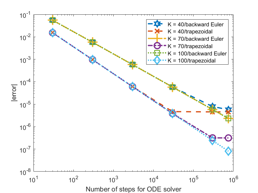
Figure 2: Maximal errors for the calculation of $D_{0}^{0.4}y(t)$ with $t\in[0,3]$ for $y(t)=t^{1.6}$ using different step sizes for the ODE solver and different numbers of quadrature nodes.

The findings of this example can be summarized as follows:

• The trapezoidal method clearly leads to a more accurate approximation than the backward Euler method. Obviously, in view of the trapezoidal method’s higher convergence order, this behaviour is exactly what would have been expected.

• The number of quadrature points, i.e. our parameter $K$, only has a very small influence on the overall error. Therefore, one can afford to work with a relatively small value of $K$, thus significantly reducing the computational cost, without a substantial loss of accuracy.

• A comparison of the results for the trapezoidal method shows that a certain kind of saturation is reached at an error level of $4.5\cdot 10^{-6}$ for $K=40$, i.e. we do not achieve a better accuracy even if we continue to decrease the step size for the ODE solver. This is an indication that this level reflects the contribution of the total error caused by the quadrature formula. If a smaller error is required, one therefore needs to use more quadrature nodes. For example, choosing $K=70$ leads to a saturation level of approximately $3.2\cdot 10^{-7}$. This indicates that the saturation level might be proportional to $K^{-0.6}$, leading to the conjecture that the exponent of $K$ in this expression could be related to the smoothness properties of the function $y$ (note that the function $y^{\prime}$ that appears in the formulas which describe our algorithm satisfies a Lipschitz condition of order $0.6$).

  The fact that this phenomenon is hardly visible if the backward Euler method is used is due to the fact that this ODE solver has a larger error which only just about reaches this range for the chosen step sizes. It would be possible to more clearly observe a similar behaviour if the step sizes were reduced even more.

We have also used a number of other test cases; the behaviour has usually been very similar. Also, the findings of [7] for a significantly different method based on a related fundamental approach point into the same direction. In our future work, we will attempt to provide a thorough analysis of the approximation properties of methods of this type that should confirm the experimental results.

References

- [1] Baffet D.: A Gauss-Jacobi Kernel Compression Scheme for Fractional Differential Equations. J. Sci. Comput. 79 (2019), 227–248, DOI 10.1007/s10915-018-0848-x
- [2] Birk C., Song C.: An Improved Non-classical Method for the Solution of Fractional Differential Equations. Comput. Mech. 46 (2010), 721–734, DOI 10.1007/s00466-010-0510-4
- [3] Chatterjee A.: Statistical Origins of Fractional Derivatives in Viscoelasticity. J. Sound Vibrations 284 (2005), 1239–1245
- [4] Davis P. J., Rabinowitz P.: Methods of Numerical Integration, 2nd ed. Academic Press, San Diego (1984)
- [5] Diethelm K.: An Investigation of Some Nonclassical Methods for the Numerical Approximation of Caputo-type Fractional Derivatives. Numer. Algorithms 47 (2008), 361–390
- [6] Diethelm K.: The Analysis of Fractional Differential Equations. Springer, Berlin (2010), DOI 10.1007/978-3-642-14574-2
- [7] Diethelm K.: Fast Solution Methods for Fractional Differential Equations in the Modeling of Viscoelastic Materials. To appear in Proc. 9th International Conference on Systems and Control (ICSC 2021); Preprint: arXiv:2111.02782
- [8] Diethelm K., Ford N. J., Freed A. D.: A Predictor-Corrector Approach for the Numerical Solution of Fractional Differential Equations. Nonlinear Dynam. 29 (2002), 3–22
- [9] Diethelm K., Ford N. J., Freed A. D.: Detailed Error Analysis for a Fractional Adams Method. Numer. Algorithms 36 (2004), 31–52
- [10] Diethelm K., Freed A. D.: An Efficient Algorithm for the Evaluation of Convolution Integrals. Computers Math. Applic. 51 (2006), 51–72
- [11] Diethelm K., Kiryakova V., Luchko Y., Machado J. A. T., Tarasov V. E.: Trends, Directions for Further Research, and Some Open Problems of Fractional Calculus. To appear in Nonlinear Dynam., DOI 10.1007/s11071-021-07158-9
- [12] Ford N. J., Simpson A. C.: The Numerical Solution of Fractional Differential Equations: Speed Versus Accuracy. Numer. Algorithms 26 (2001), 333–346
- [13] Garrappa R.: Numerical Solution of Fractional Differential Equations: A Survey and a Software Tutorial. Mathematics 6 (2018), 16, DOI 10.3390/math6020016
- [14] Hairer E., Lubich C., Schlichte M.: Fast Numerical Solution of Nonlinear Volterra Convolution Equations. SIAM J. Sci. Stat. Comput. 6 (1985), 532–541, DOI 10.1137/0906037
- [15] Hairer E., Lubich C., Schlichte M.: Fast Numerical Solution of Weakly Singular Volterra Integral Equations. J. Comput. Appl. Math. 23 (1988), 87–98, DOI 10.1016/0377-0427(88)90332-9
- [16] Hairer E., Wanner G.: Solving Ordinary Differential Equations II, 2nd revised edition, corrected second printing. Springer, Berlin (2002), DOI 10.1007/978-3-642-05221-7
- [17] Hinze M., Schmidt A., Leine R. I.: Numerical Solution of Fractional-order Ordinary Differential Equations Using the Reformulated Infinite State Representation. Fract. Calc. Appl. Anal. 22 (2019), 1321–1350, DOI 10.1515/fca-2019-0070
- [18] Li J.-R.: A Fast Time Stepping Method for Evaluating Fractional Integrals. SIAM J. Sci. Comput. 31 (2010), 4696–4714
- [19] Lubich C.: Fractional Linear Multistep Methods for Abel-Volterra Integral Equations of the Second Kind. Math. Comput. 45 (1985), 463–469
- [20] Lubich C.: Discretized Fractional Calculus. SIAM J. Math. Anal. 17 (1986), 704–719
- [21] Lubinsky D. S.: A Survey of Weighted Polynomial Approximation with Exponential Weights. Surv. Approx. Theory 3 (2007), 1–105
- [22] McLean W.: Exponential Sum Approximations for . In: Dick J., Kuo F. Y., Woźniakowski H. (eds.): Contemporary Computational Mathematics, pp. 911–930. Springer, Cham (2018)
- [23] Montseny G.: Diffusive Representation of Pseudo-Differential Time-Operators. ESAIM Proc. 5 (1998), 159–175
- [24] Schmidt A., Gaul L.: On a Critique of a Numerical Scheme for the Calculation of Fractionally Damped Dynamical Systems. Mech. Res. Commun. 33 (2006), 99–107
- [25] Singh S. J., Chatterjee A.: Galerkin Projections and Finite Elements for Fractional Order Derivatives. Nonlinear Dynam. 45 (2006), 183–206
- [26] Szegő G.: Orthogonal Polynomials, 4th edition, Amer. Math. Soc., Providence (1975)
- [27] Trinks C., Ruge P.: Treatment of Dynamic Systems with Fractional Derivatives Without Evaluating Memory-integrals. Comput. Mech. 29 (2002), 471–476
- [28] Yuan L., Agrawal O. P.: A Numerical Scheme for Dynamic Systems Containing Fractional Derivatives. J. Vibration Acoust. 124 (2002), 321–324
- [29] Zhang W., Capilnasiu A., Sommer G., Holzapfel G. A., Nordsletten D.: An Efficient and Accurate Method for Modeling Nonlinear Fractional Viscoelastic Biomaterials. Comput. Methods Appl. Mech. Eng. 362 (2020), 112834, DOI 10.1016/j.cma.2020.112834