FedADMM: A Robust Federated Deep Learning Framework with Adaptivity to System Heterogeneity

Abstract

Federated Learning (FL) is an emerging framework for distributed processing of large data volumes by edge devices subject to limited communication bandwidths, heterogeneity in data distributions and computational resources, as well as privacy considerations. In this paper, we introduce a new FL protocol termed FedADMM based on primal-dual optimization. The proposed method leverages dual variables to tackle statistical heterogeneity, and accommodates system heterogeneity by tolerating variable amount of work performed by clients. FedADMM maintains identical communication costs per round as FedAvg/Prox, and generalizes them via the augmented Lagrangian. A convergence proof is established for nonconvex objectives, under no restrictions in terms of data dissimilarity or number of participants per round of the algorithm. We demonstrate the merits through extensive experiments on real datasets, under both IID and non-IID data distributions across clients. FedADMM consistently outperforms all baseline methods in terms of communication efficiency, with the number of rounds needed to reach a prescribed accuracy reduced by up to $87\%$. The algorithm effectively adapts to heterogeneous data distributions through the use of dual variables, without the need for hyperparameter tuning, and its advantages are more pronounced in large-scale systems.

I Introduction

The abundance of data constitutes the fuel for the proliferation of Machine Learning (ML) in all aspects of life. In many applications, data are being generated in large quantities in a distributed fashion: for instance, crowdsourcing, mobile phones, autonomous vehicles, medical centers, distributed sensors in smart grids, to name but a few. The sheer size of the data alongside the urge to protect personal privacy prevent traditional distributed machine learning practices from being directly applied. The well-studied framework of data-center distributed learning [1, 2] often involves maneuvering raw data from machine to machine, which not only violates privacy restrictions but also becomes infeasible when limited networking resources fail to cope with large data sizes. Besides, the rapid increase of the computational power of personal devices such as smartphones surges pushing computation to the edge as opposed to the cloud.

Federated Learning (FL) was proposed in [3, 4] as a new paradigm for tackling large-scale distributed machine learning problems with distinct features compared to the data-center setting: (i) massive client population; (ii) limited communication resources; (iii) low device participation rate and unreliable connections; (iv) stringent privacy considerations. A canonical setting of FL is shown in Fig. 1, where a server coordinates with clients to compute a global ML model.

Figure 1: Architecture of FL. Active clients ① download the current global model from the server, ② perform local training based on their data, ③ upload an update message to the central server. Server ④ aggregates clients’ updates to form a new global model.

The introduction of this framework was carried in [4], wherein the authors proposed FedAvg as the main algorithm. At each round of FedAvg, a small fraction of clients is selected and each selected client downloads the global model. The selected clients then proceed to update the model by running SGD using their local data, and upload the updated model to the server. Finally, a new global model is obtained by the server through averaging the updated models. Despite the fact that FedAvg is arguably the most widely adopted method of choice for FL, it does not address either system heterogeneity or statistical heterogeneity. Specifically, FedAvg does not explicitly handle the straggler problem in a heterogeneous network: the process may stall in the face of unreliable network connections or client unavailability. Moreover, FedAvg may diverge when data distributions across clients violate the IID (independent and identically distributed) assumption [4, 5, 6, 7].

The authors in [8] proposed FedProx, which augments a proximal term to the local training problem to counter possible divergence resulting from statistical heterogeneity. Additionally, this method accommodates system heterogeneity by allowing variable amount of work at each selected client. Nevertheless, the performance of FedProx is sensitive to the selection of the proximal coefficient, whose tuning depends on prior knowledge on statistical distributions and system sizes [8]. SCAFFOLD [9] introduces client and server control variates, which effectively act as tracking variables for local and global information. It is reported to outperform FedAvg/Prox through utilizing the similarity of data across clients, but its communication cost per round is doubled due to the extra control variates.

Another branch of work has roots in primal-dual optimization methods, such as Generalized Method of Multipliers and Alternating Direction Method of Multipliers (ADMM) [10, 11, 12] that have enjoyed much success in distributed optimization. Such methods provide a general framework which not only encompasses a wide range of objectives—such as low-rank matrix completion, nonconvex neural network training, and reinforcement learning [13, 14, 15]—but it can also be tailored for specific application demands, such as event-triggered communication and inexact computing [16, 17, 18, 19, 20].

In this paper, we propose FedADMM, a primal-dual algorithm that automatically adapts to data heterogeneity while achieving significant convergence speedup compared to the state-of-the-art. Each round of FedADMM involves a small fraction of clients and allows a plethora of computing choices for per user. A distinctive attribute of FedADMM is the use of dual variables to guide the local training process (see Section III-A for detailed discussion), which effectively account for automatic adaptation to data distributions without tuning. This specifically addresses a key challenge encountered in the FL setting known as avoiding client drift: local training performed at clients has to be carefully designed according to statistical variations so as to prevent the model from overfitting to a specific selected client’s data. We note that compared to SCAFFOLD, where the acceleration is achieved through storing and communicating the control variates that capture local gradient information, FedADMM maintains the exact same communication cost per round as FedAvg/Prox. Using a limited amount of extra storage for the dual variables (which is readily available and inexpensive in practical FL scenarios), FedADMM effectively harnesses the capabilities of edge devices and achieves significant communication and computation savings due to the automated adaptation to statistical variations.

Contributions:

We present a new framework for Federated Learning, termed FedADMM.

• Through the use of local augmented Lagrangian and dual variables, FedADMM addresses both system and statistical heterogeneity.

• By introducing a generalized server update step size, the proposed method achieves a fine balance between convergence speed and robustness against oscillations.

• We establish a convergence rate of $\mathcal{O}(\tfrac{1}{T})+\mathcal{O}(1)$ for the proposed algorithm under less restrictive assumptions than the state-of-the-art. Moreover, this rate matches the complexity lower bound for reaching an $\varepsilon$-stationary solution.

• A crucial feature of FedADMM is that no restrictions are imposed on the client activation scheme other than the necessary infinitely often participation. This is achieved by clients solving local augmented Lagrangian subproblems that are strongly convex, which ensures progress is made without diverging under a most general participation scheme.

• We have conducted numerous experiments on distributed neural network training from real datasets in both IID and non-IID settings, which attest that FedADMM achieves high accuracy in fewer rounds compared to the state-of-the-art (an average $72\%$ and a maximum $87\%$ of communication savings over the best performing baseline are reported over several datasets, population sizes, and both statistical and system heterogeneity). Notably, the advantages of FedADMM are most pronounced in large-scale networks with heterogeneous data distributions.

II Related work

Existing primal-dual algorithms for FL include FedHybrid [21] and FedPD [22]. FedHybrid is a synchronous method (requiring all clients to update at each round) that tackles system heterogeneity by separating clients into two groups, one performing gradient updates and the other Newton updates. However, this setting does not encapsulate federated deep learning (Newton’s method is not applicable for large neural networks, while also convergence is established under strong convexity assumptions). FedPD employs gradient-based (GD or SGD) local training with variable amount of work at clients. Similar to our proposed method, it invokes dual variables to capture the discrepancy between local models and the global model. Nevertheless, FedPD adopts full client participation, in that (i) all clients update their local models and dual variables at each round and (ii) at each round, with fixed probability, either all clients communicate with the server to update the global model, or there is no communication. Therefore, the frequency of updating the global model is limited by the probability of communicating. We note that all clients in FedHybrid/PD are continuously engaged in computing, which incurs large computational overhead to devices. Moreover, requiring all clients to communicate at the same time not only imposes strict requirements on clients’ availability and network bandwidth, but also exacerbates the straggler problem (where the server has to wait for the slowest client before proceeding to the next round).

In contrast, our proposed solution (i) applies partial client participation for both computation and communication, (ii) updates the global model at each round, and (iii) leverages tracking in the global model update rule (which accounts for accelerated convergence with smoother paths). The server in FedADMM communicates with a fraction of clients during each round and clients only perform local training when selected. We establish convergence without restrictions on statistical heterogeneity among the networks, or the fraction of participating users. This is in contradistinction to the analysis of other baseline methods [8, 5, 23] which requires assumptions on data dissimilarity that may be unrealistic in practices when data are individually generated by each client [24, 25, 26]. Our proposed method has close connections to randomized ADMM [27], which in the FL setting amounts to randomly activating clients and the server. However, it requires that subproblems to be solved exactly, which may be impractical in consideration of heterogeneous hardware conditions and data volumes. On the other hand, FedADMM accounts for inexact solutions from local problems and allows variable amount of training performed at clients (quantified by a tunable parameter). Another related line of work is termed asynchronous ADMM [28, 29, 30], whose focus is on alleviating the straggler problem mentioned earlier. However, assumptions imposed therein such as the bounded delay assumption (i.e., each user needs to be active at least once every some number of rounds) may never be satisfied in FL settings.

Figure 2: FedADMM on selected clients during the $t$-th round. Selected clients ① download the current server model, ② carry local training and update their dual variables (Alg. 1, line 6), ③ upload update messages (Alg. 1, line 8). Server ④ aggregates messages from selected edge clients to update the global model.

III Algorithm

The objective of FL is cast as a loss minimization problem:

$$\underset{\theta\in\mathbb{R}^{d}}{\mathrm{minimize}}\ \ \sum_{i=1}^{m}f_{i}(\theta),$$ (1)

where $m$ is the number of clients and $f_{i}(\theta)=\tfrac{\alpha_{i}}{n_{i}}\sum_{k=1}^{n_{i}}l_{ik}(\theta)$ captures the weighted local training loss. Common choices of weights include $\alpha_{i}=\frac{n_{i}}{n}$, where $n=\sum_{i=1}^{m}n_{i}$ (i.e., weighting clients proportionally to their data volumes) or $\alpha_{i}=1$ (i.e., equal weights, which serves to avoid overfitting to clients with more data, and is also the choice in our experiments). The goal of FL is to solve (1) over model parameter $\theta$ using data distributed across clients. In contrast to data-center distributed machine learning, communication is the bottleneck for FL applications. The large number of clients in federated systems renders infeasible synchronous communication (i.e., all clients communicating with the server at a given round) with large message sizes; this is due to bandwidth limitations and the existence of stragglers. Moreover, the large data volumes involved along with the leakage of personal information from raw data prevents the server from collecting local data for centralized processing. Thus, a candidate algorithm for FL should meet the following requirements: (i) communication efficiency; (ii) low client participation rate per round; (iii) handling both system and statistical heterogeneity; (iv) no transmission of client raw data. We proceed to present FedADMM whose design meets all these guidelines.

III-A Proposed Algorithm: FedADMM

We first reformulate (1) into the following consensus setting that is more suitable for our development:

$$\underset{w_{i},\theta\in\mathbb{R}^{d}}{\mathrm{minimize}}\ \ \sum_{i=1}^{m}f_{i}(w_{i}),\ \ \text{s.t.}\ \ w_{i}=\theta,\ \ \forall i\in[m].$$ (2)

Problem (2) is equivalent to (1) in the sense that the optimal solutions coincide. This formulation naturally fits into the FL setting, where $w_{i}$ can be interpreted as the local model held by client $i$ and $\theta$ as the global model held by the server.

Algorithm 1 FedADMM

1:Input: Total number of rounds $T$, server step size $\eta$, proximal coefficient $\rho$.

2:for $t=0,1,\dots,T-1$ do

3:     Server selects $S^{t}\subset[m]$

4:Clients: // In parallel

5:     for $i\in S^{t}$ do

6:         download $\theta^{t}$ from the server

7:         $(w_{i}^{t+1},y_{i}^{t+1})\leftarrow$ClientUpdate($i,\theta^{t}$)

8:         compute update message $\Delta_{i}^{t}$ as in (4)

9:         upload $\Delta_{i}^{t}$ to the server

10:     end for

11:Server:

12:     $\theta^{t+1}\leftarrow\theta^{t}+\frac{\eta}{\left|S^{t}\right|}\sum_{i\in S^{t}}\Delta_{i}^{t}$

13:end for

14:

15:ClientUpdate$(i,\theta)$: // Store $w_{i}$ and $y_{i}$

16:Input: Local epoch number $E_{i}$, client learning rate $\eta_{i}$.

17:create batches $\mathcal{B}$

18:for $k=0,1,\dots,E_{i}-1$ do

19:     for batch $b\in\mathcal{B}$ do

20:         compute batch gradient $\nabla f_{i}(w_{i},b)$

21:         $w_{i}\leftarrow w_{i}-\eta_{i}\big{(}\nabla f_{i}(w_{i},b)+y_{i}+\rho(w_{i}-\theta)\big{)}$

22:     end for

23:end for

24:$y_{i}\leftarrow y_{i}+\rho(w_{i}-\theta)$

25:return $w_{i},y_{i}$

At the beginning of the $t$-th round, a subset of clients is selected (denoted as $S^{t}$) and each selected client downloads the server model $\theta^{t}$. We note that a favorable attribute of FedADMM lies in that client selection (step 3 of Alg. 1) can be carried by any mechanism (e.g., an adaptive rule based on device operating conditions such as energy and bandwidth) as long as it guarantees non-zero probability of participation. Local training is performed to update the client model as $w_{i}^{t+1}\approx\underset{w_{i}}{\text{argmin}}\,\,\mathcal{L}_{i}(w_{i},y_{i}^{t},\theta^{t})$, where

$$\mathcal{L}_{i}(w_{i},y_{i}^{t},\theta^{t})=f_{i}(w_{i})+(y_{i}^{t})^{\top}(w_{i}-\theta^{t})+\frac{\rho}{2}\norm{w_{i}-\theta^{t}}^{2}.$$ (3)

We note that $y_{i}^{t}\in\mathbb{R}^{d}$ is the local dual variable held by client $i$ and $\rho>0$ is the coefficient of the quadratic term. Both the dual variables and the quadratic term serve to strike a balance between updating model parameters using local data while staying consistent with the server model (which serves to incorporate information from all participants). We note that FedProx [8] similarly solves (3) with $y_{i}^{t}\equiv 0$. While this provides some level of safeguard against client drift, competitive performance of FedProx relies on careful tuning of $\rho$ [8, 9]. The addition of the dual variables helps FedADMM to achieve automatic adaptation to heterogeneous data distributions and significantly alleviates the problem of hyperparameter tuning; we postpone detailed discussions on dual variables to the end of this section. In addition to the local model update (Alg. 1, lines 14-19), the dual variable for each selected client is updated in line 20. We combine the primal and dual variables to what we call augmented model $\big{(}w_{i}+\frac{1}{\rho}y_{i}\big{)}$, and use $\Delta_{i}^{t}\in\mathbb{R}^{d}$ to denote the update message of client $i$ to the server, that is the difference between successive augmented models:

$$\Delta_{i}^{t}=\left(w_{i}^{t+1}+\tfrac{1}{\rho}y_{i}^{t+1}\right)-\left(w_{i}^{t}+\tfrac{1}{\rho}y_{i}^{t}\right).$$ (4)

The server updates the global model after gathering update messages from selected clients as:

$$\theta^{t+1}=\theta^{t}+\tfrac{\eta}{\absolutevalue{S^{t}}}\sum_{i\in S^{t}}\Delta_{i}^{t},$$ (5)

where $\eta>0$ is the server gathering step size. Different choices of $\eta$ are suitable for different scenarios in terms of scale of the system and statistical variations. We empirically observe that setting $\eta=1$ gives rise to fast training speed, while setting $\eta=\absolutevalue{S^{t}}/m$ helps to eliminate oscillatory behaviors when significant heterogeneity is detected. In contrast to FedAvg/Prox, where the global model is updated using information only from the current models of clients $i\in S^{t}$, the server in FedADMM effectively incorporates past information. This is accomplished through the tracking update rule in (5) and serves to provide additional safeguard against oscillations emanating from heterogeneous data and the stochastic nature of the algorithm.

We emphasize that in a practical scenario (3) is not required to be solved exactly, but instead the updated local model $w_{i}^{t+1}$ can be computed inexactly in the following sense:

$$\norm{\nabla_{w_{i}}\mathcal{L}_{i}(w_{i}^{t+1},y_{i}^{t},\theta^{t})}^{2}\leq\varepsilon_{i},$$ (6)

where $\varepsilon_{i}\geq 0$ prescribes the local accuracy. Note that a variable accuracy level is allowed for different clients (a smaller $\varepsilon_{i}$ corresponds to a more accurate solution). This is useful since user devices in FL systems feature varying hardware conditions such as computational power, network connectivity, battery level, etc. For the sake of simplicity and comparison with baseline methods, this is done in Algorithm 1 by running $E_{i}$ epochs of SGD to compute $w_{i}^{t+1}$ (line 14); the equivalence with (6) emanates from the fact that local subproblems (3) are strongly convex. Nevertheless, other updating schemes are also feasible such as gradient descent and quasi-Newton updates like L-BFGS. Therefore, we accommodate system heterogeneity by letting clients decide to perform different amount of work according to their local environments. Finally, we note that each client in FedADMM holds the primal-dual pair $(w_{i},y_{i})$, while it only communicates the augmented model difference $\Delta_{i}^{t}$, i.e., the communication cost per round is identical with FedAvg and FedProx.

Dual variables: Contrary to primal only methods (FedAvg/Prox and SCAFFOLD), the augmented Lagrangian $\mathcal{L}_{i}$ is used for the training of local model parameters $w_{i}$. Invoking the augmented Lagrangian is effective for two reasons: (i) by a proper selection of the quadratic proximal coefficient $\rho$, it is possible to make $\mathcal{L}_{i}$ in (3) strongly convex with respect to $w_{i}$ (this is true even for non-convex $f_{i}$); therefore, theoretical guarantees for reaching a prescribed local accuracy level $\varepsilon_{i}$ in (6) are readily obtainable. (ii) the dual variable $y_{i}$ in (3), in addition to penalizing the discrepancy between the local model and the global model, further provides a quantitative measure of the benefit brought by letting local models be different from the server model during the initial stage of training. To illustrate, note that the stationary points for each subproblem, i.e., the solutions to $\nabla f_{i}(\theta)=0$, tend to be different from one another, especially in FL settings with heterogeneous data distributions across clients. The stationary condition of (1), $\sum_{i=1}^{m}\nabla f_{i}(\theta^{\star})=0$, indicates that the cost reduction by following any given $-\nabla f_{i}(\theta^{\star})$ may be partly or entirely cancelled by the increase of other $f_{j}(\theta^{\star}),j\neq i$. This is encoded within the KKT conditions for problem (2): $\nabla f_{i}(w_{i}^{\star})+y_{i}^{\star}=0$ for all $i\in[m]$ and $\sum_{i=1}^{m}y_{i}^{\star}=0$. Therefore, $y_{i}\in\mathbb{R}^{d}$ can be interpreted as a signed “price vector” (with entries being positive or negative) which not only quantifies the cost of $w_{i}^{t+1}$ being different from $\theta^{t}$, but also provides a direction of the adjustments needed for agreement. This effectively achieves an automatic adaptation to statistical variations in that it safeguards against client drift, i.e., $w_{i}$ converging to client optima.

III-B Connections with Existing Work

We show how FedADMM generalizes FedAvg and FedProx. Recall the augmented Lagrangian defined in (3). By setting $y_{i}\equiv 0$ (i.e., also omitting line 20 in Alg. 1), we recover the local training problem of FedProx. If additionally $\rho$ is set to $0$, one recovers the local training problem of FedAvg. The main motivation of these two terms is to tackle a fundamental challenge reminiscent of FL, i.e., the balance between (i) extensive local training (aiming for faster convergence speed of the entire FL process, thus a reduction of the total number of communication rounds), and (ii) deterring client models from overfitting to their local data. In addition to the quadratic proximal term introduced in FedProx, FedADMM further employs dual variables, whose merits in guiding the update of local models $w_{i}$ were discussed in the prequel. We note that SCAFFOLD similarly stores additional variables at clients and the server to counter statistical variations. However, the variable introduced therein can not be combined into a single message (as is accomplished with our augmented model and update messages in (4)), whence SCAFFOLD doubles the size of the uploading message to the server. On the other hand, FedADMM only stores an additional vector at clients but maintains the exact same upload size. To this end, we believe FedADMM is an effective scheme for harnessing local device capabilities to alleviate communication costs, which constitutes a primordial motivation for FL. Extensive experiments illustrate a substantial reduction of communication in all test cases ($72\%$ on average) over the best performing baseline.

IV Analysis

In this section, we provide the convergence analysis for FedADMM. We adopt the following standard assumptions.
Assumption 1. Each local loss function $f_{i}(\cdot)$ is $L$-Lipschitz smooth, i.e., $\forall\,w,w^{\prime}\in\mathbb{R}^{d}$, the following inequality holds:

$$\norm{\nabla f_{i}(w)-\nabla f_{i}(w^{\prime})}\leq L\norm{w-w^{\prime}},\,\,i\in[m].$$

Assumption 2. The objective of problem (1) is lower bounded, i.e., there exists $f^{\star}\in\mathbb{R}$ such that $\sum_{i=1}^{m}f_{i}(w)\geq f^{\star},\forall\,w\in\mathbb{R}^{d}$.

The above assumptions are minimally restrictive, since loss functions are typically non-negative and the structure of the deep neural networks considered in the experiments ascertains Lipschitz smoothness. We further denote the aggregated Lagrangian as $\mathcal{L}=\sum_{i=1}^{m}\mathcal{L}_{i}$ and we define a non-negative function $V\left(\{w^{t}_{i}\},\{y^{t}_{i}\},\theta^{t}\right)$ to measure the optimality gap:

$$V^{t}:=\norm{\nabla_{\theta}\mathcal{L}^{t}}^{2}+\sum_{i=1}^{m}\left(\norm{\nabla_{w_{i}}\mathcal{L}^{t}}^{2}+\norm{w_{i}^{t}-\theta^{t}}^{2}\right).$$ (7)

Since each term of $V^{t}$ is non-negative, $V^{t}=0$ if and only if $\norm{\nabla_{\theta}\mathcal{L}^{t}}=\norm{\nabla_{w_{i}}\mathcal{L}_{i}^{t}}=\norm{w_{i}^{t}-\theta}=0$, $\forall\,i$. It can be further verified that these terms are $0$ if and only if a stationary solution of (2) is reached.

Theorem 1. Let assumptions 1 and 2 hold. Assume each client has a probability of being selected at each round that is lower bounded by a positive constant $p_{\mathrm{min}}>0$. Let $\eta=\absolutevalue{S^{t}}/m$, and select $\rho>(1+\sqrt{5})L$, then the following holds:

$$\tfrac{1}{mT}\sum_{t=0}^{T-1}\mathbb{E}[V^{t}]\leq\tfrac{1}{mT}\tfrac{c_{2}}{c_{1}}\left(\mathcal{L}^{0}-f^{\star}+\tfrac{m}{2L}\varepsilon_{\mathrm{max}}\right)+c_{3}\varepsilon_{\mathrm{max}},$$ (8)

where $\varepsilon_{\mathrm{max}}=\max_{i}\,\varepsilon_{i}$, $c_{1}=p_{\mathrm{min}}\left(\tfrac{\rho-2L}{2}-\tfrac{2L^{2}}{\rho}\right)$, $c_{2}=3(L^{2}+\rho^{2})+2(1+\tfrac{2L^{2}}{\rho^{2}})$, and $c_{3}=\left(3+\tfrac{16}{\rho^{2}}+\tfrac{c_{2}}{c_{1}}\cdot\tfrac{\rho+16L}{2L\rho}\right)$.

Remark 1: Note that the loss functions considered in our experiments admit $L=\mathcal{O}(1)$, i.e., the Lipschitz constant does not scale with the client population (this is because the input data are uniformly bounded, e.g., images). To reach an $\varepsilon$-exact solution in such cases, Theorem 1 suggests a complexity of $\mathcal{O}(1/\varepsilon p_{\mathrm{min}})$ by setting $\rho\in\mathcal{O}(L)=\mathcal{O}(1)$. We compare the convergence property of FedADMM with other baselines in Table I. Note that only FedProx and FedPD among baseline methods enjoy the same favorable dependency on solution accuracy as FedADMM, i.e., $\mathcal{O}(1/\varepsilon)$. However, they both impose additional restrictive conditions to achieve this. In particular, FedProx requires selecting $S>B^{2}$, where $B$ is a measure of data dissimilarity across users as in (9). This imposes constraints on minimum number of active clients. On the contrary, our analysis for FedADMM establishes convergence under arbitrary client participation and does not require (9) (i.e., $B=\infty$ is also acceptable). Besides, FedPD requires all clients to communicate simultaneously (i.e., it does not allow partial client participation), which we believe is unrealistic for large networks where stragglers and unavailability of machines is ubiquitous. On the other hand, SCAFFOLD and FedADMM both allow arbitrarily large values of $G$ (gradient norm bound as in (10)) and $B$, but SCAFFOLD doubles the communication cost per client compared to FedADMM.

TABLE I: Number of communication rounds required to reach an $\varepsilon$-stationary solution. Constants $B,G$ measure data dissimilarity and boundedness of gradients in (9) and (10) respectively, $m$ is the total number of clients, and $S$ denotes the number of active clients.

Method	Number of communication rounds
FedAvg[4, 9]	$\mathcal{O}(1/\varepsilon^{2}\cdot(m-S)/mS+G/\varepsilon^{3/2}+B^{2}/\varepsilon)$
FedProx1[8]	$\mathcal{O}(B^{2}/\varepsilon)$
SCAFFOLD[9]	$\mathcal{O}(1/\varepsilon^{2}+1/\varepsilon\cdot(m/S)^{\tfrac{2}{3}})$
FedPD2 [22]	$\mathcal{O}(1/\varepsilon)$
FedADMM	$\mathcal{O}(1/\varepsilon\cdot(m/S))$
1FedProx requires $S>B^{2}$ to ensure convergence.
2FedPD requires all clients to communicate at the same time.

Remark 2: For simplicity, we stated Theorem 1 assuming users are active with a non-zero probability at each round. In fact, the weaker condition is needed that each client is active infinitely often, which is necessary for the correctness of any iterative distributed algorithm (otherwise some clients are ignored). This in turn allows for a general activation scheme and thus incurs no lower bound on minimum number of active clients per round. The reason that this is possible is the introduction of dual variables and the quadratic penalty term which alleviate the effect of possible unbalanced client activation. Further insight can be gained by inspecting the inequality (31), where we derive the expected decrement of the augmented Lagrangian. This suggests that any activation scheme can be supported by our analysis: using time dependent participating probability $p_{i}^{t}$ for each client, our convergence proof carries as long as $\sum_{t=1}^{\infty}p_{i}^{t}=\infty$ (infinitely often participation) by invoking the Borel-Cantelli Lemma II.

We emphasize that our choice of $\rho$ can be made without any a priori knowledge on system sizes, number of participating clients, and statistical variation across clients. The dynamic nature of FL makes such selection rule of the hyperparameter useful and practical. This is corroborated by our experiments in Section V which shows that FedADMM performs well with constant $\rho$ in settings with different system sizes and data distributions.

In addition to the assumptions 1-2, the following conditions have been imposed when analyzing existing state-of-the-art methods. Our analysis does not require any of these conditions.
(Data dissimilarity) The local client loss functions satisfy:

$$\sum_{i=1}^{m}\norm{\nabla f_{i}(w)}^{2}\leq\norm{\sum_{i=1}^{m}\nabla f_{i}(w)}^{2}B^{2},$$ (9)

for some constant $B$ and all $w\in\{w\,|\,\norm{\sum_{i=1}^{m}\nabla f_{i}(w)}^{2}>\varepsilon\}$. Note that since the accuracy $\varepsilon$ can be chosen arbitrarily small, this condition is restrictive as it would effectively force $B\to\infty$ as $\varepsilon\to 0$, unless data distributions are similar across clients. In other words, in scenarios where accurate solutions are pursued and when data distributions are heterogeneous, the analysis in [8] dictates that all clients need to participate in each round (which is highly undesirable in FL) when such an assumption is imposed.
(Bounded Gradient) There exists a constant $G$ that uniformly bounds the client loss function gradient, i.e.,

$$\norm{\nabla f_{i}(w_{i}^{t})}\leq G,\,\,\forall w_{i}^{t}\in\mathbb{R}^{d}.$$ (10)

The above assumption was imposed in [23, 5] to analyze FedAvg for bounding iterate paths during local training. However, it may be unrealistic to impose a uniform bound in the face of large populations and data heterogeneity.

TABLE II: Experimental Setup.

Model	# of para	Dataset	Target Accuracy
CNN 1	1,663,370	MNIST	97%
		FMNIST	80%
CNN 2	1,105,098	CIFAR-10	45%

TABLE III: Comparison of number of communication rounds along with the speedup relative to FedSGD to reach a target accuracy (100+ indicates the target accuracy was not reached in 100 rounds). For MNIST dataset with 100 clients, $E=5,B=200$ was used for both IID and non-IID data distributions. In all 1,000 client settings, we set $E=20,B=10$ for the non-IID case, and $E=20,B=\infty$ (full-batch) for the IID case. Reduction of number of communication rounds using FedADMM is computed over the best baseline method in each experiment.

	MNIST (100 clients)		MNIST (1,000 clients)		FMNIST (1,000 clients)		CIFAR-10 (1,000 clients)
	IID	Non-IID	IID	Non-IID	IID	Non-IID	IID	Non-IID
FedSGD	297	250	201	269	390	530	186	202
FedADMM	$\mathbf{10(29.7\times)}$	$\mathbf{33(7.6\times)}$	$\mathbf{8(25.1\times)}$	$\mathbf{13(20.7\times)}$	$\mathbf{3(130.0\times)}$	$\mathbf{7(75.7\times)}$	$\mathbf{7(26.6\times)}$	$\mathbf{9(22.4\times)}$
FedAvg	19($15.6\times$)	77($3.2\times$)	61($3.3\times$)	73($3.7\times$)	10($39.0\times$)	33($16.1\times$)	24($7.8\times$)	50($4.0\times$)
FedProx	29($10.2\times$)	100+	78($2.6\times$)	100+	14($27.9\times$)	61($8.7\times$)	32($5.8\times$)	68($3.0\times$)
SCAFFOLD	27($11.0\times$)	76($3.3\times$)	61($3.3\times$)	84($3.2\times$)	12($32.5\times$)	40($13.3\times$)	37($5.0\times$)	100+
Reduction	47.4 %	56.6%	86.9%	82.2%	70.0%	78.8%	70.8%	82.0%

V Experiments

We conducted experiments on three datasets, namely MNIST [34], Fashion MNIST (FMNIST) [35], and CIFAR-10 [36]. We compare our proposed method against FedSGD, FedAvg [4], FedProx [8], and SCAFFOLD [9] using two popular CNN models [34, 4] with two convolutional layers each and number of parameters as detailed in Table II. We do not compare against FedHybrid [21] and FedPD [22], since they are both involve communication rounds that require participation of all users, which we deem unrealistic for large-scale FL scenarios. In brief, our experiments unravel three main findings: (i) FedADMM achieves high accuracy in both IID and non-IID settings within substantially fewer rounds, which translates to large communication savings; (ii) FedADMM features robust convergence against both statistical and system heterogeneity, and requires no hyperparameter tuning across the IID and non-IID settings. This is in contrast to FedProx whose proximal coefficient needs to be carefully chosen according to data dissimilarity, which is difficult to assess in a practical scenario; (iii) FedADMM outperforms all baseline methods in all test scenarios, with the advantages being most pronounced in large-scale systems with heterogeneous data distributions. This is as opposed to other methods, where an improved performance is restricted to either the IID or the non-IID setting.

V-A Experimental Setup

We study ten-class image classification on three real datasets with details specified below. Two CNN models are used for our experiments, both with a convolutional module (two $5\times 5$ convolutional layers, each followed by $2\times 2$ max pooling layers), and a fully connected layer module. The input of the two models is a flattened image with dimension $784$ and $3,072$, respectively, while the output for both is a class label from $0$ to $9$. Table II summarizes the datasets, model sizes, and target accuracies used in our experiments. We denote $E$ as the local epoch number, $B$ as the local batch size, and $C$ as the fraction of clients that participate in the training process during each round. All experiments are implemented in PyTorch on a system with 2 Intel^® Xeon^® Silver 4210 CPUs and 2 NVIDIA^® Tesla^® V100S GPUs. Clients are selected uniformly at random during each global round, and the number of participating clients is set to $10\%$ ($C=0.1$) of total clients in all cases, while SGD was chosen as the local solver in all cases. This was done for the sake of comparison with the baselines, but our framework allows for arbitrary client participation and local solver. The system heterogeneity (i.e., variable computational capabilities across clients) is captured by letting each client select the local epoch number uniformly between $1$ and $E$ in FedADMM as well as in FedProx. The number of local epochs for FedAvg and SCAFFOLD are fixed to be $E$; this was done in order to compare against baselines in their principal description. We adopt random initialization for the global model in all algorithms, zero initialization for dual variables in FedADMM, and zero initialization for control variates in SCAFFOLD (as recommended). Recall that the use of control variates doubles the upload cost of SCAFFOLD compared to other baselines. We set the server gathering step size $\eta$ to be 1 unless otherwise specified and present all results averaged over five runs. The code is available at: github.com/YonghaiGong/FedADMM.

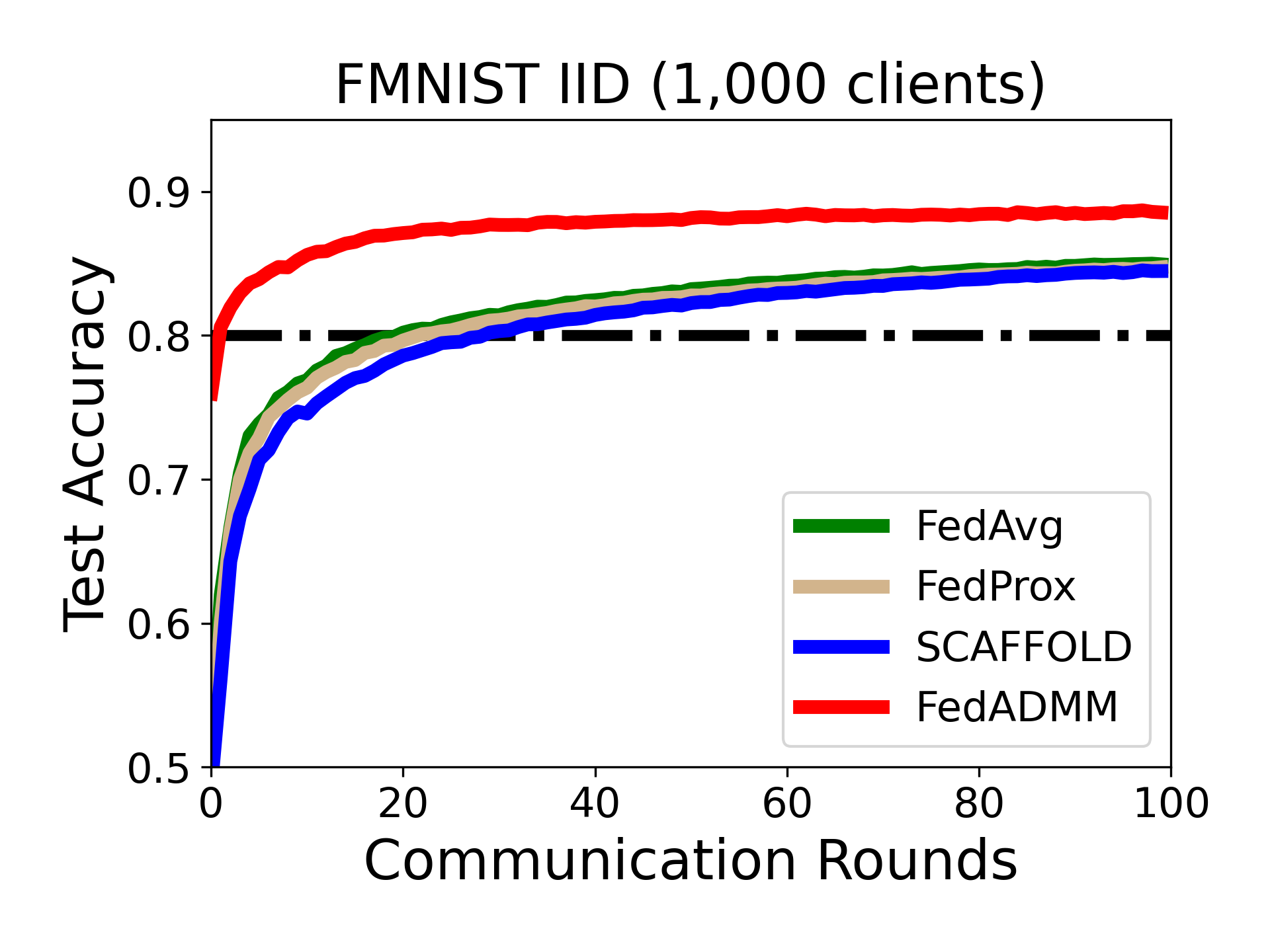
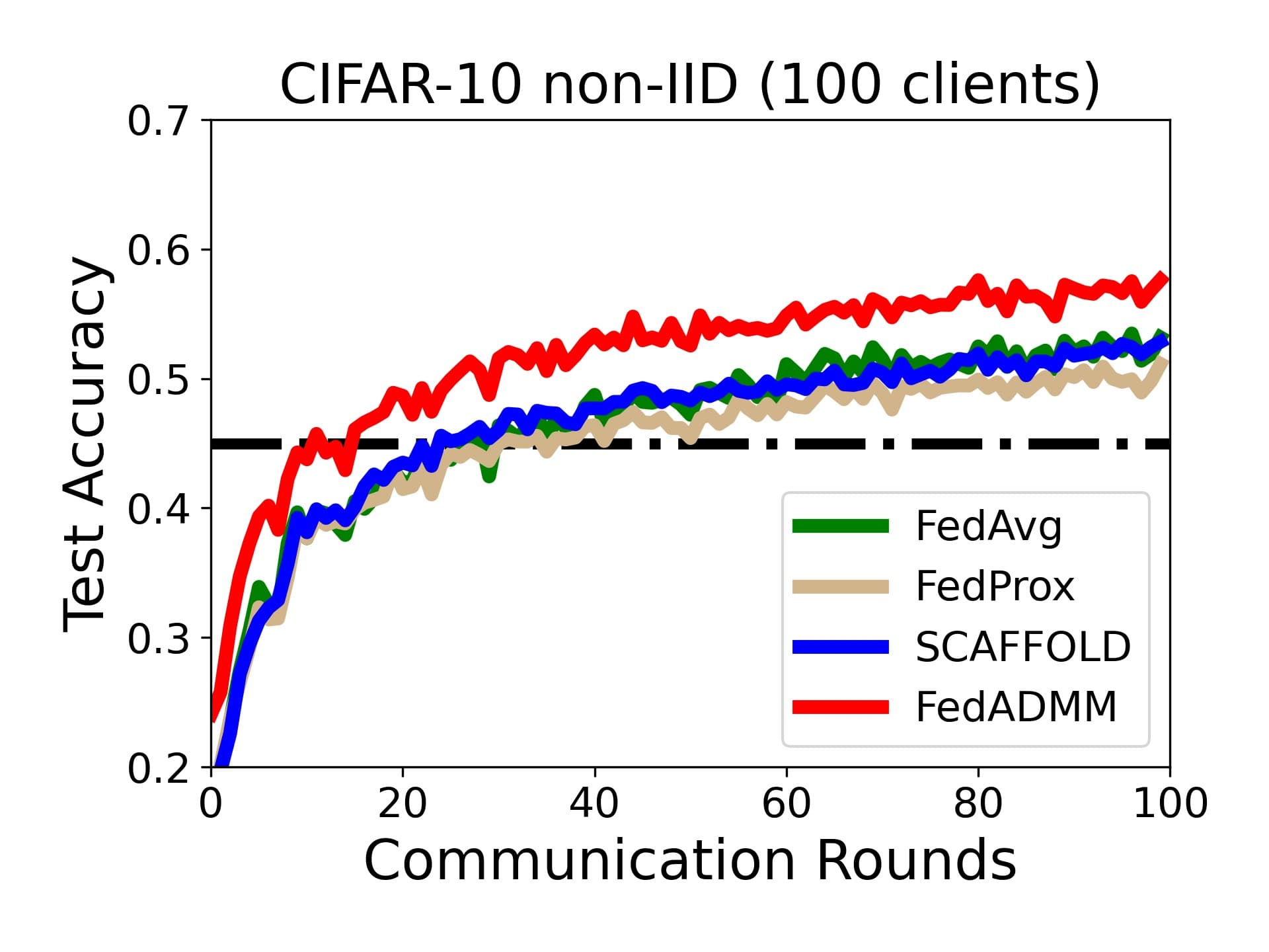
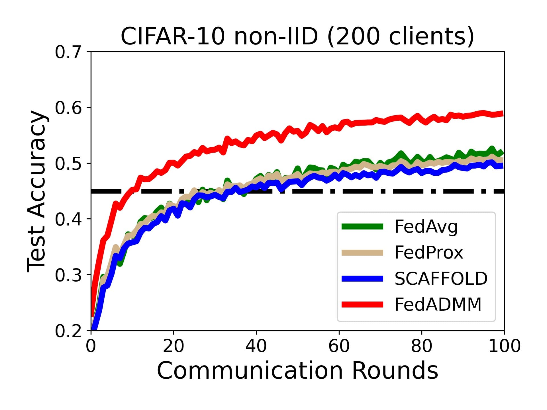
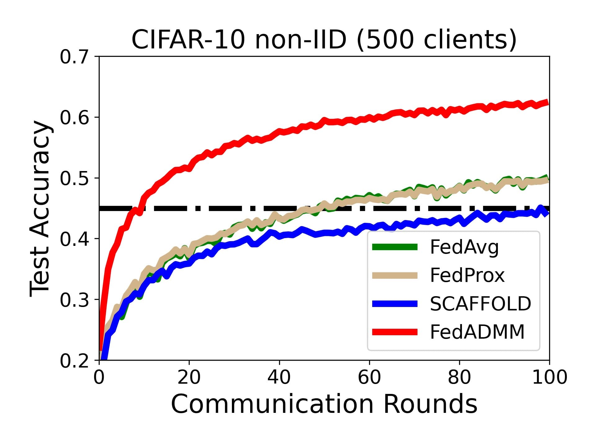
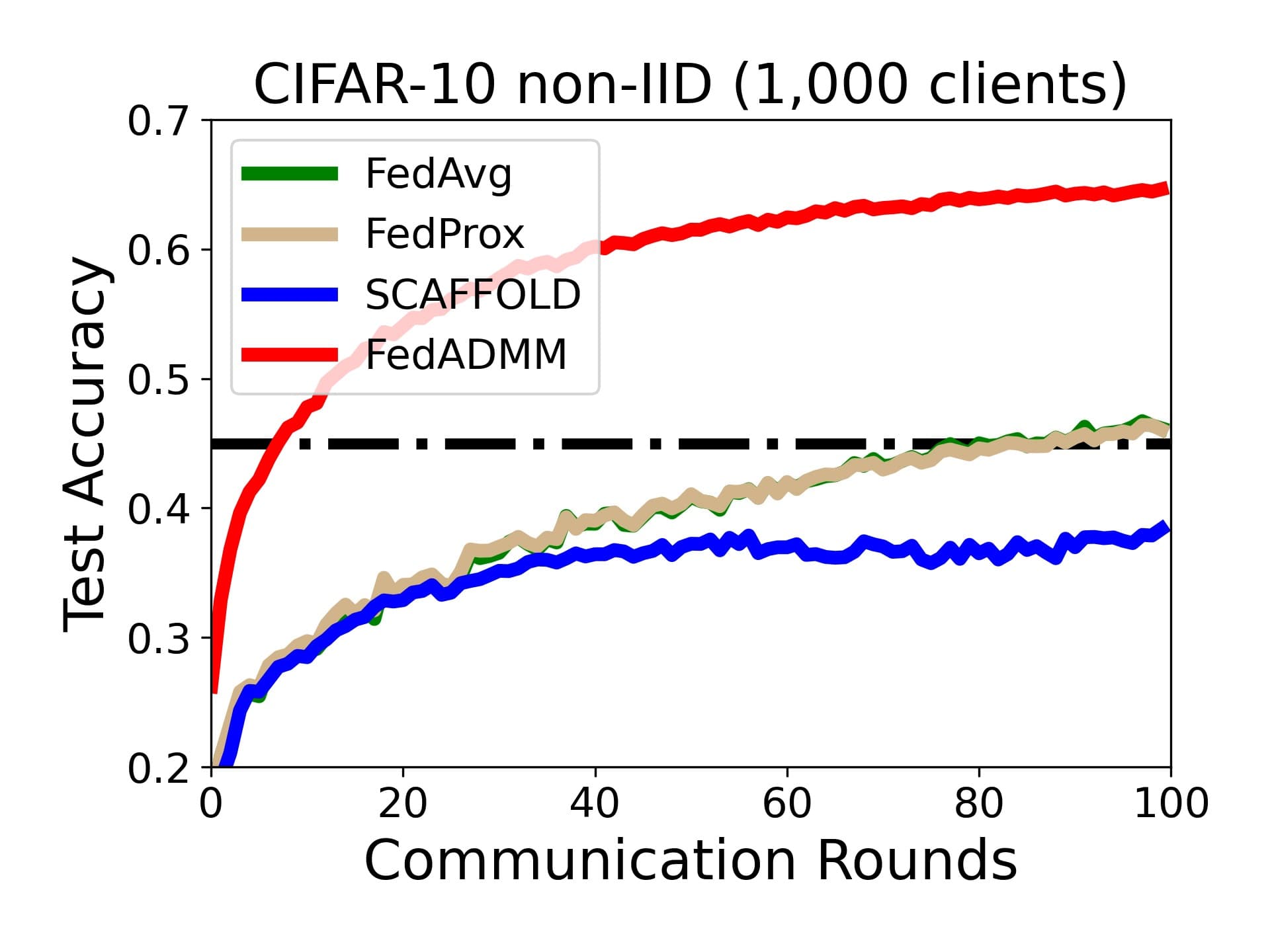
Figure 3: Convergence paths in systems with variable number of users (prescribed accuracies of $80\%$ for FMNIST and $45\%$ for CIFAR-10 are plotted as black dashed lines). We test how performance varies with fixed hyperparameters (tuned for best performance in the 100-client setting) for different system scales. We conclude that the performance gap of FedADMM increases with the client population.

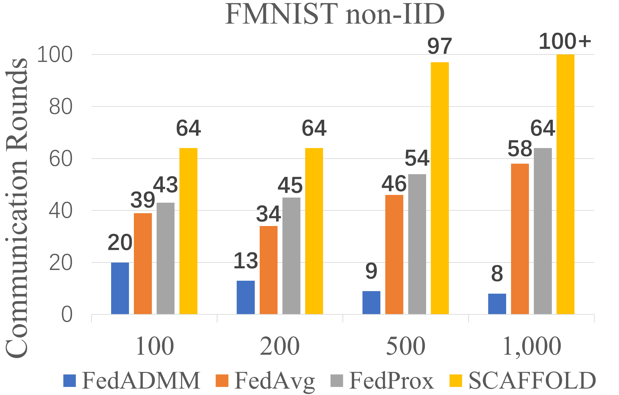
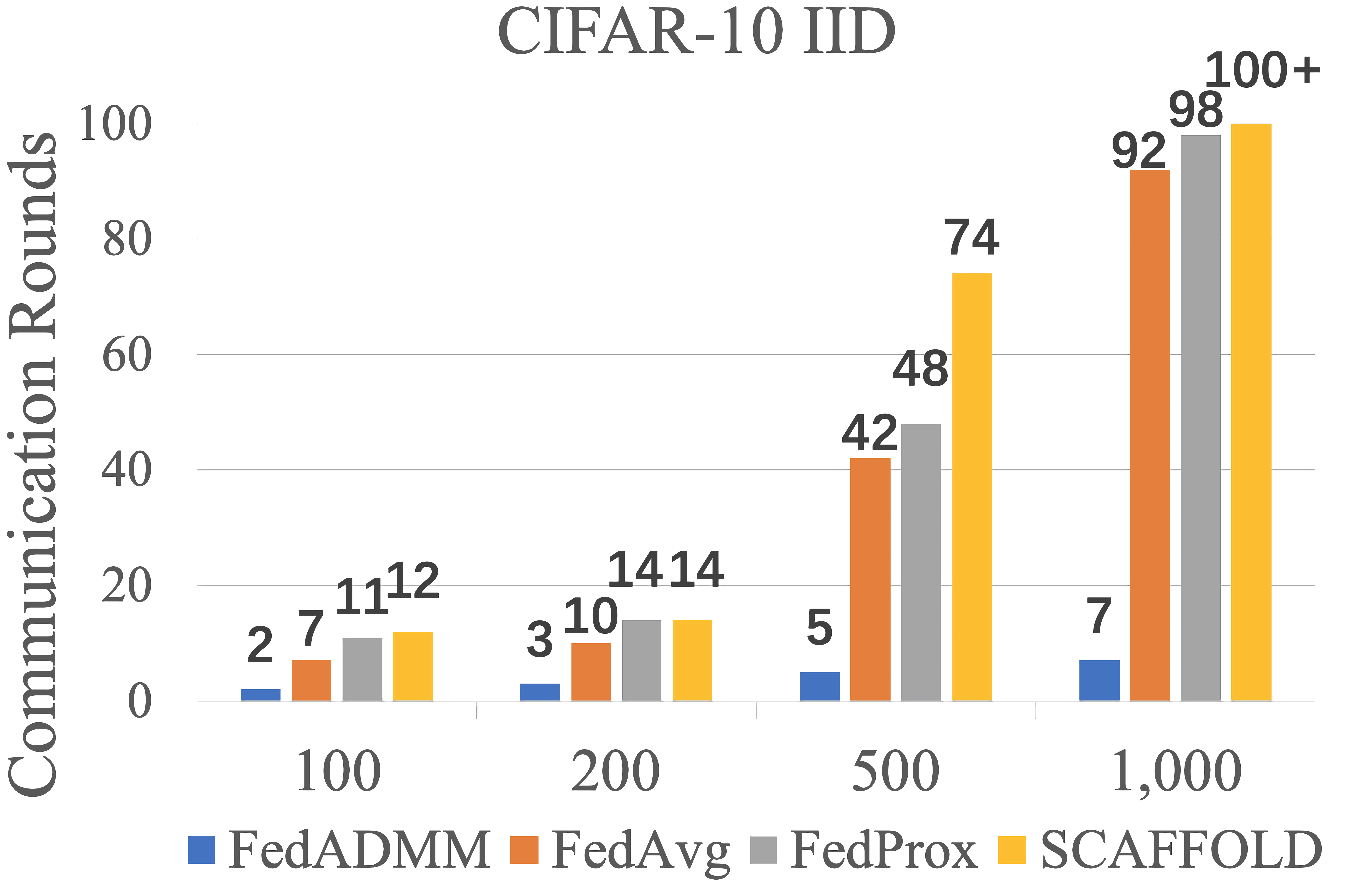
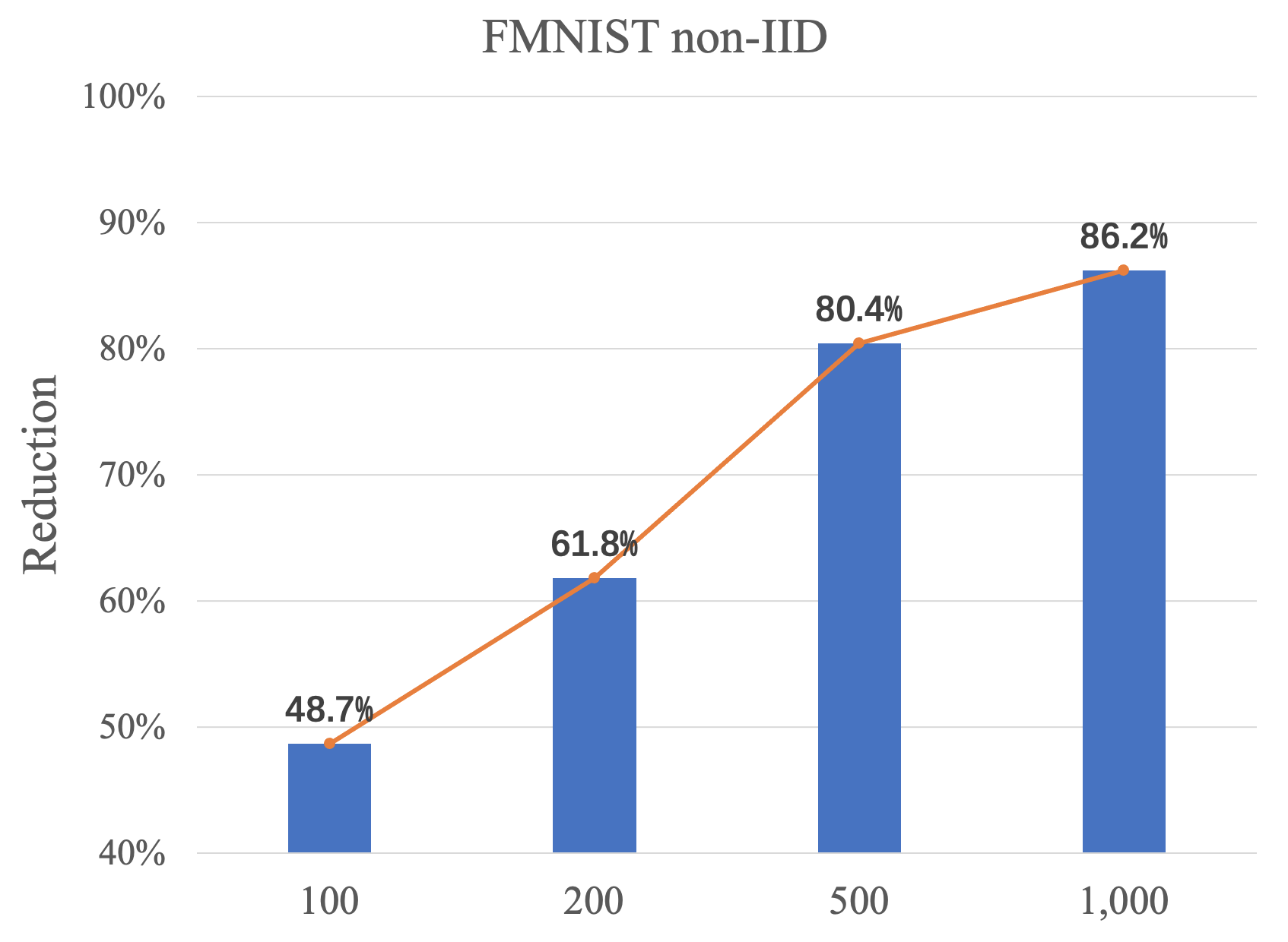
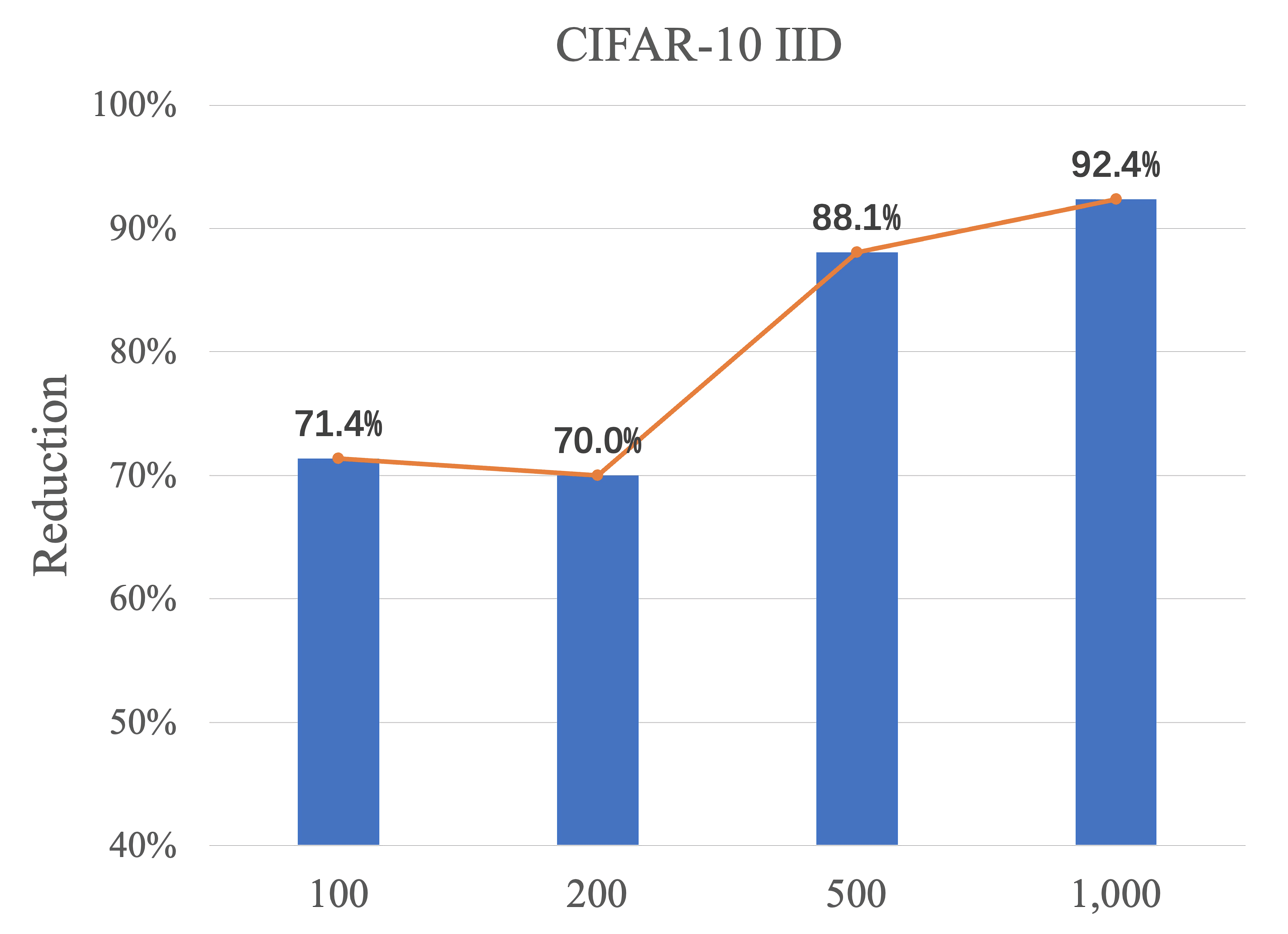
Figure 4: Number of rounds to reach a prescribed accuracy for variable client population along with the reduction of FedADMM over the best baseline method.

Data Distribution. For the IID setting, data are evenly distributed to clients. In contrast, to account for data heterogeneity (non-IID setting), we first arrange the training data by label and then distribute them evenly into shards: each client is assigned two shards uniformly at random. We note that this is a rather extreme representative of data heterogeneity, since clients tend to overfit to the specific classes of assigned data.
Hyperparameters. The learning rates of the local SGD solver for all algorithms are selected from the candidate set $\{0.01,0.1,0.2,0.5\}$ for best performance. Recall that both FedADMM and FedProx make use of a quadratic penalty term and require the setting of hyperparameter $\rho$. It has been observed in [8], [9], and is further supported in our experiments, that careful tuning of $\rho$ is required to achieve the best performance for FedProx (see discussion on Proximal Parameter $\rho$ in Section V-B). For fairness, we fixed $\rho=0.1$ for FedProx except for Table III, where $\rho$ is selected from the candidate set $\{0.001,0.01,0.1,1\}$ to test for its best performance. In contrast, FedADMM outperforms all baselines with fixed $\rho=0.01$ (empirically fixed) in all experiments. This is in full alignment with our theoretical analysis (see Theorem 1 and Remark 1) that suggests that $\rho$ can be set as constant, independent of system size and data distributions.

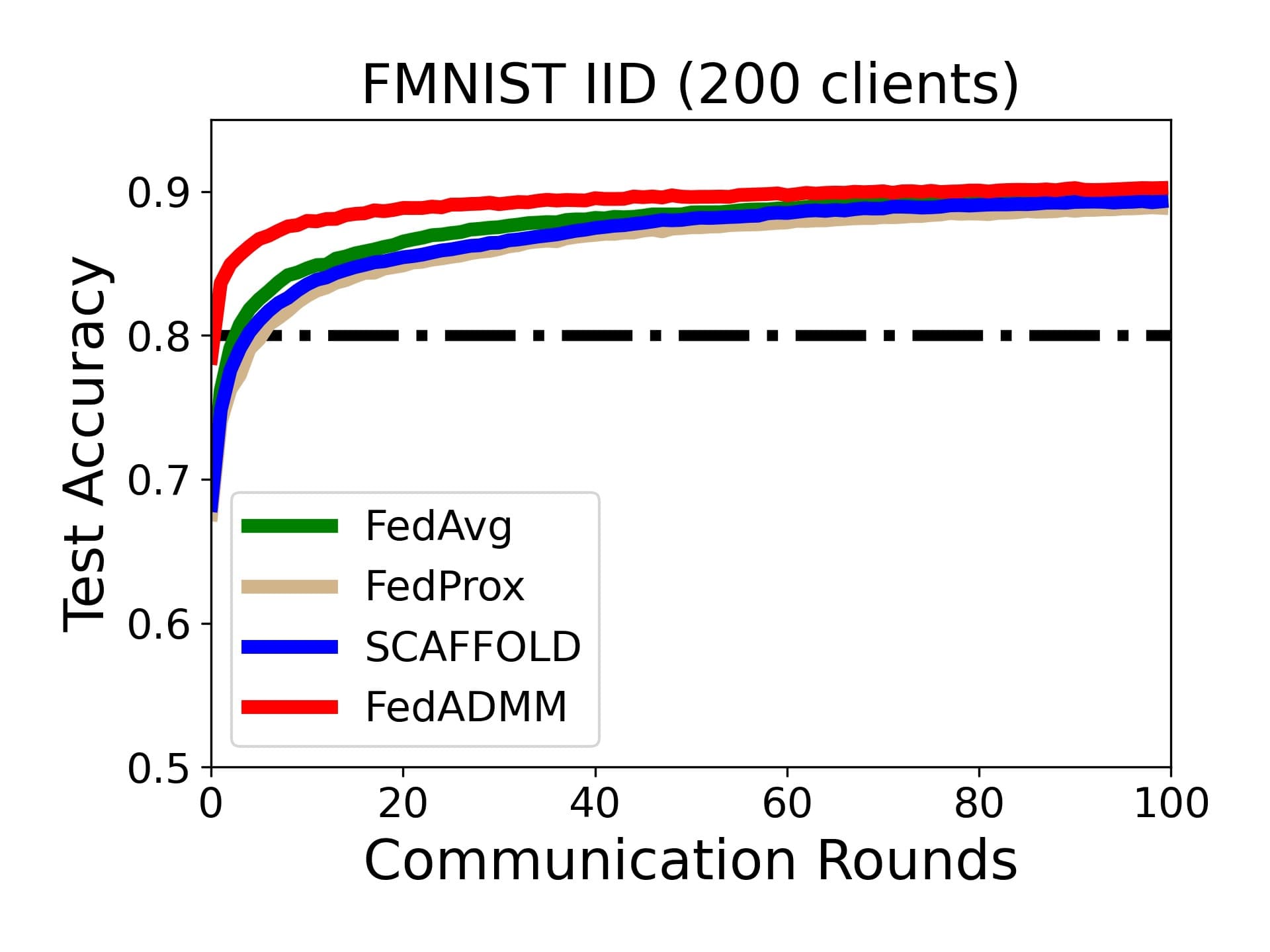
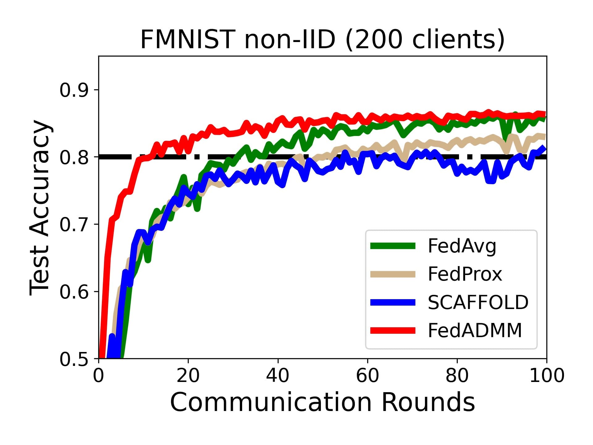
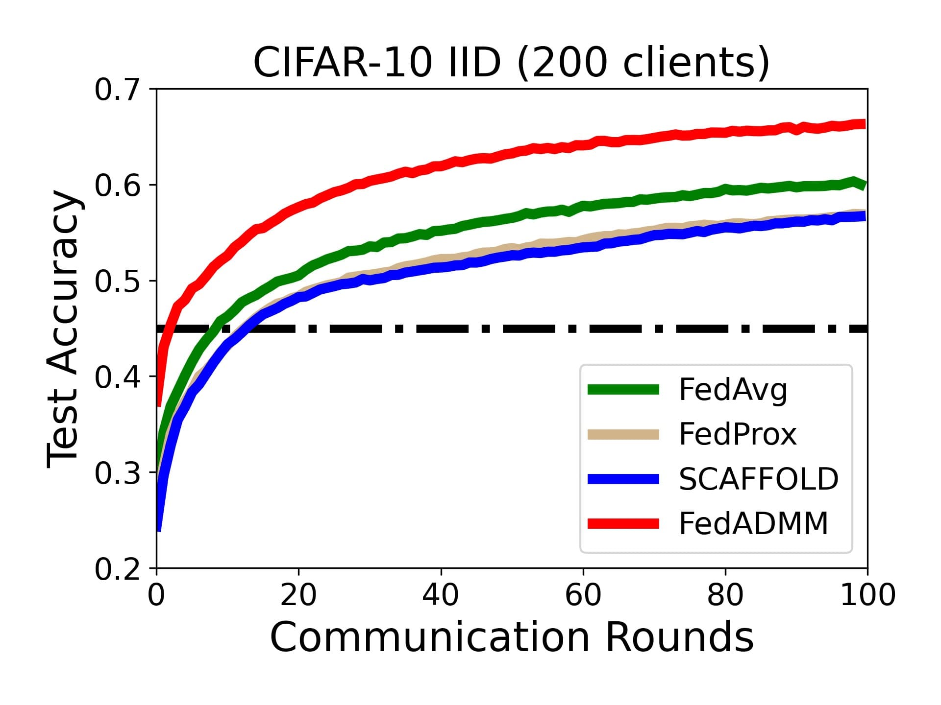
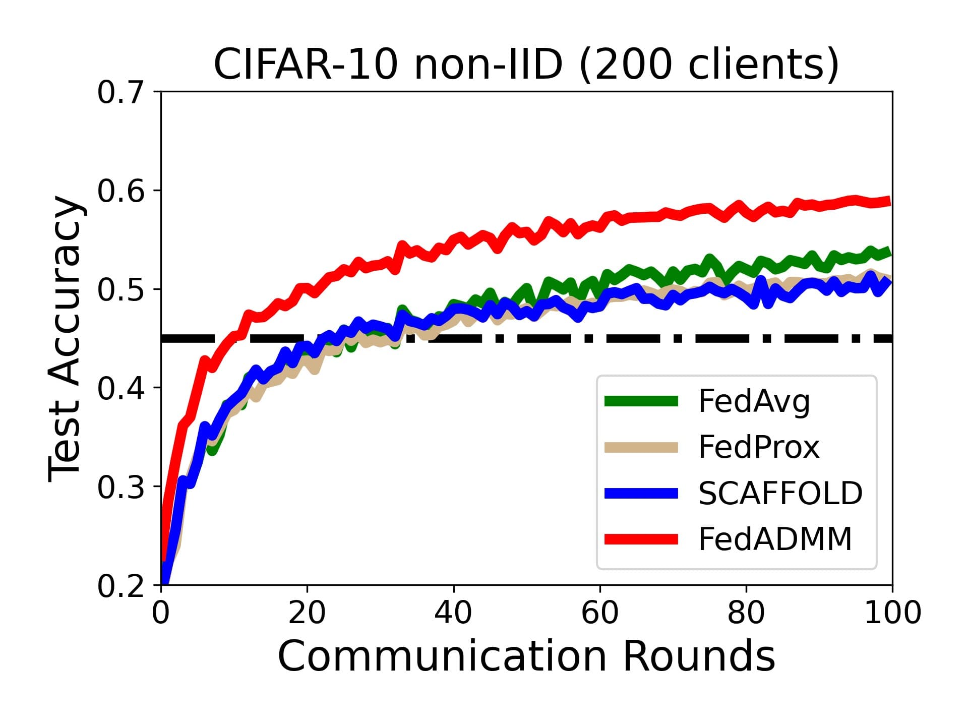
Figure 5: Comparison of adaptability to heterogeneous data. Target accuracy is $80\%$ for FMNIST and $45\%$ for CIFAR-10. For both cases, $m=200$, $E=10$, $B=50$. In FedADMM, we fix the local learning rates to $0.1$ and $\rho=0.01$, while other algorithms are tuned for best performance. In all scenarios, FedADMM consistently outperforms all baseline methods even with no hyperparameter tuning.

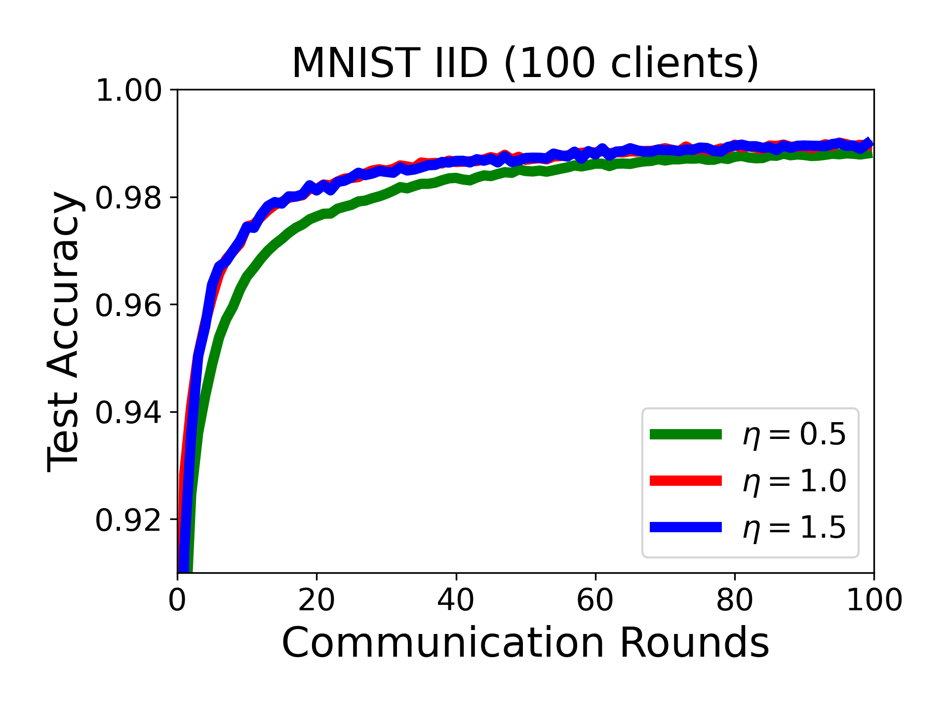
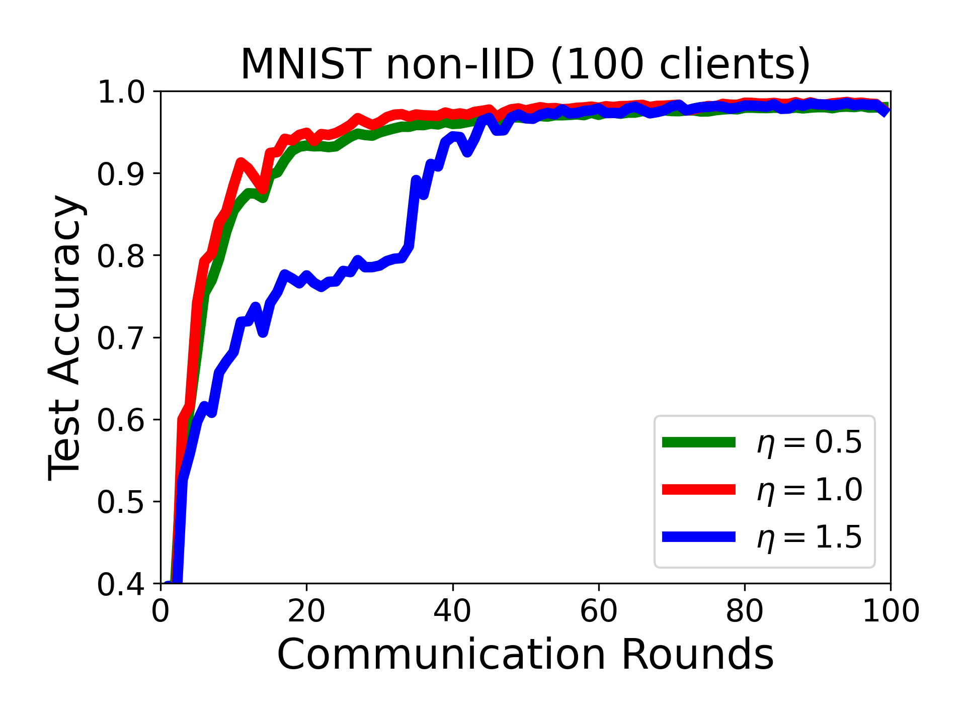
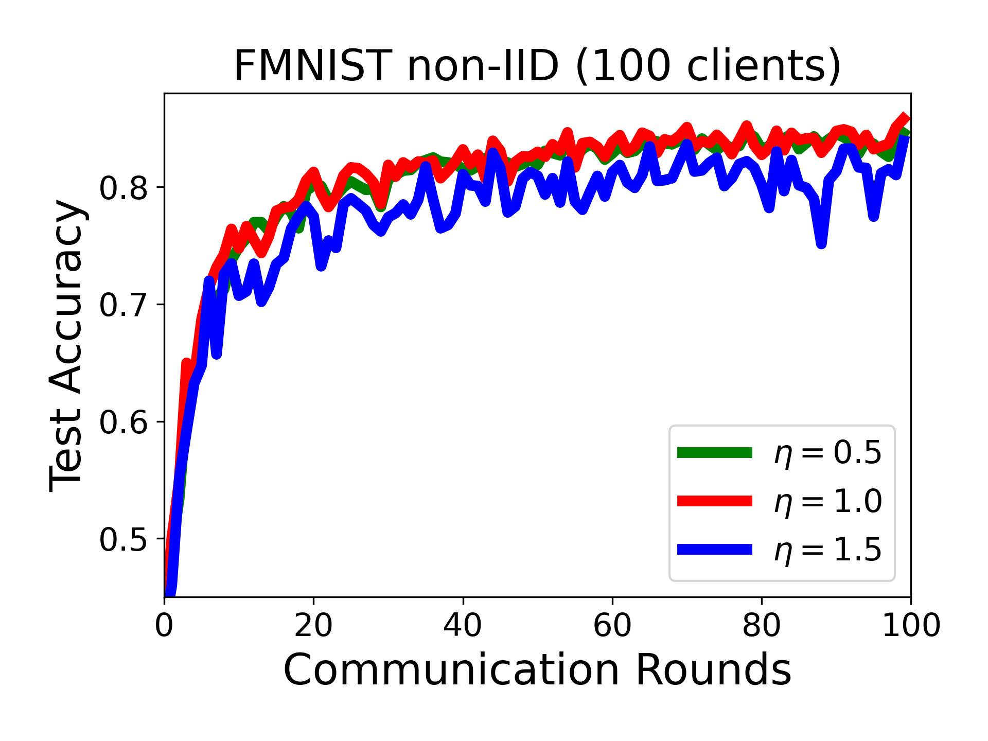
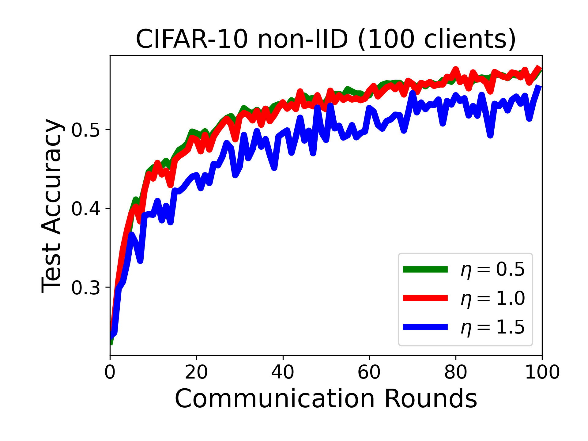
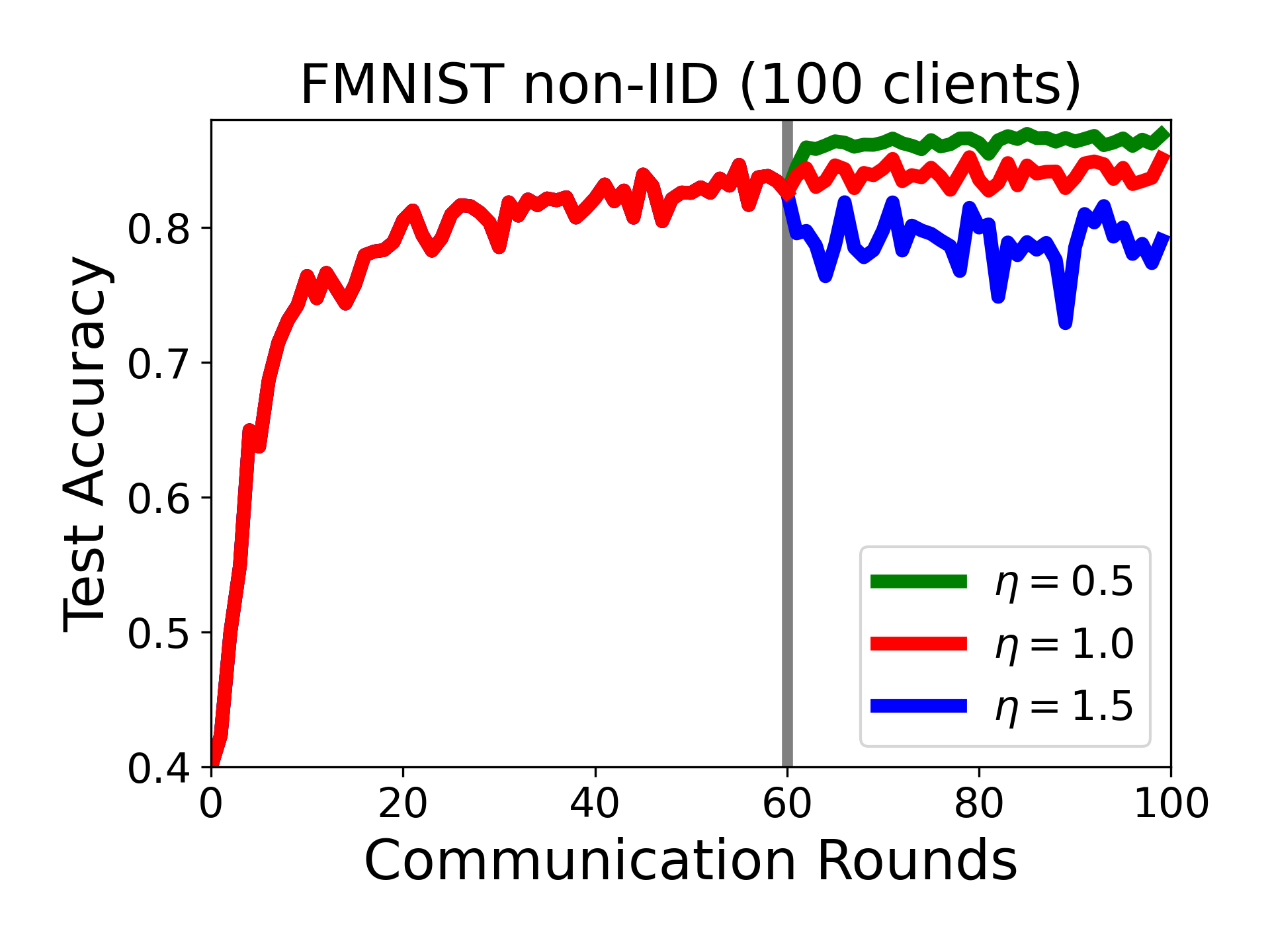
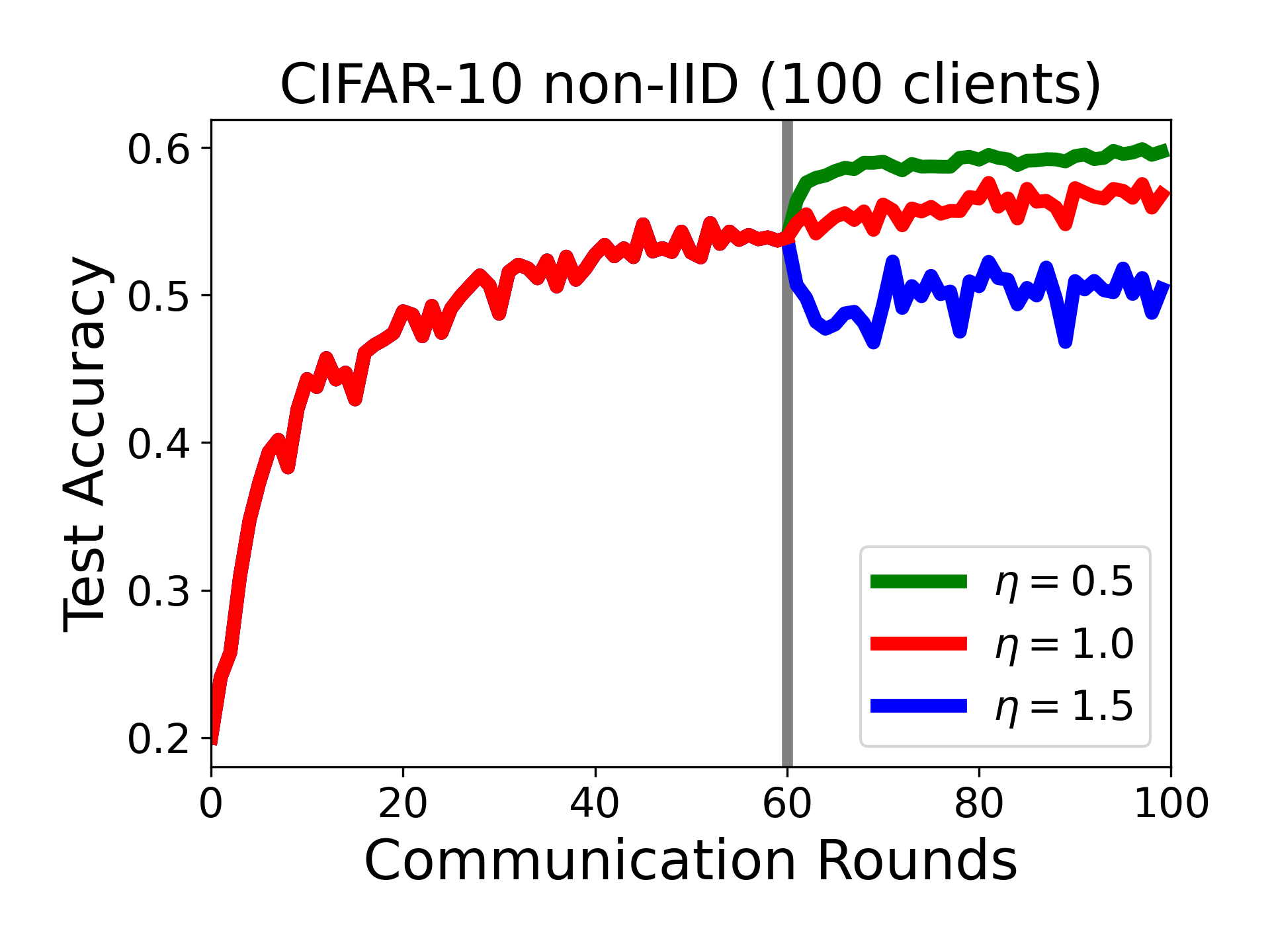
Figure 6: Performance comparison using different server step sizes for FedADMM. The vertical line indicates the point of when the step size is adjusted. The nominal step size $\eta=1.0$ yields consistent performance, while a decrease of the step size at later stages of the process can further improve the algorithm.

V-B Experimental Results

We first demonstrate the communication efficiency of FedADMM by comparing the number of rounds needed to reach a prescribed target accuracy. The results accompanied by a detailed description are summarized in Table III. We note that FedADMM consistently outperforms all baseline methods in all cases tested. In specific, the communication savings achieved by FedADMM compared to the best baseline method in each case averages $72\%$. Recall also that FedADMM has $50\%$ less training computation than FedAvg and SCAFFOLD in all instances, since those were tested without system heterogeneity considerations, unlike FedProx and FedADMM.

Increasing System Scale. We compare the performance of FedADMM in different system scales using the FMNIST and CIFAR-10 datasets with both IID and non-IID data distributions. We first tuned all algorithms for their best performance in the 100-client setting, and then scale up system sizes with the hyperparameters fixed. The results are illustrated in Fig. 3. Fig. 4 serves to complement Fig. 3: it considers the same datasets but for the reversed setting (IID becomes non-IID and vice versa). We keep the same fraction ($C=0.1$) of participating clients at each round, which translates to the same amount of data being used per round. Note, however, that an increase of the client population comes with the introduction of additional dual variables for FedADMM. In other words, the same amount of data is processed with more guidance, which serves to yield a larger improvement of FedADMM over baseline methods at larger scales. This favorable attribute is intensified in the non-IID setting where FedADMM is shown to achieve an effective incorporation of local information even faster. We conclude that FedADMM has formidable scalability, as also suggested by Theorem 1. In summary, the performance boost at increased scale (especially in the non-IID setting) is attributed to: (i) a higher aggregate number of information exchanges with the server, (ii) a higher total computational power in the network (albeit both at no additional cost per user), and (iii) additional dual variables, which provide extra guidance to the learning process.

Data Heterogeneity. To demonstrate the adaptability of FedADMM to heterogeneous data distributions, we fix parameters of FedADMM while tuning other methods for their best performance. Fig. 5 reveals the robust performance of FedADMM to statistical variations (with no hyperparameter tuning). This is a positive attribute for FL applications where data distributions are unpredictable and may be hard to characterize due to strict restrictions on clients’ data privacy. As discussed in Section III, the dual variables in FedADMM serve as an automatic adaptation mechanism to data heterogeneity, by quantitatively recording the discrepancy between the local model and the global model.

Server step size. We explore the effect of adjusting the server gathering step size $\eta$ in a system with 100 clients. In the left figure of the first row of Fig. 6, we observe that when data distributions are IID across clients, all choices of $\eta$ result in similar performance, with the smallest $\eta=0.5$ being slightly slower at initial stages. This is due to the fact that when data are evenly distributed among clients, more drastic updates are allowed. When data distributions are non-IID, care must be taken in incorporating local information to the global model. This is reflected by the stalling in the case of setting $\eta=1.5$. The nominal value $\eta=1.0$ showcases consistent performance in all cases. We additionally tested the effect of adjusting $\eta$ at later stages of the process (60 rounds): a decrease of the step size serves to incorporate past information in a finer fashion, thus improving the test accuracy.

TABLE IV: Number of rounds required for FedADMM to reach given accuracy ($97\%$ for MNIST and $45\%$ for CIFAR-10) with variable amount of local training.

		$E=1$	$E=5$	$E=10$
MNIST	IID	27	10	6
	non-IID	56	33	32
CIFAR-10	IID	24	12	10
	non-IID	30	14	11

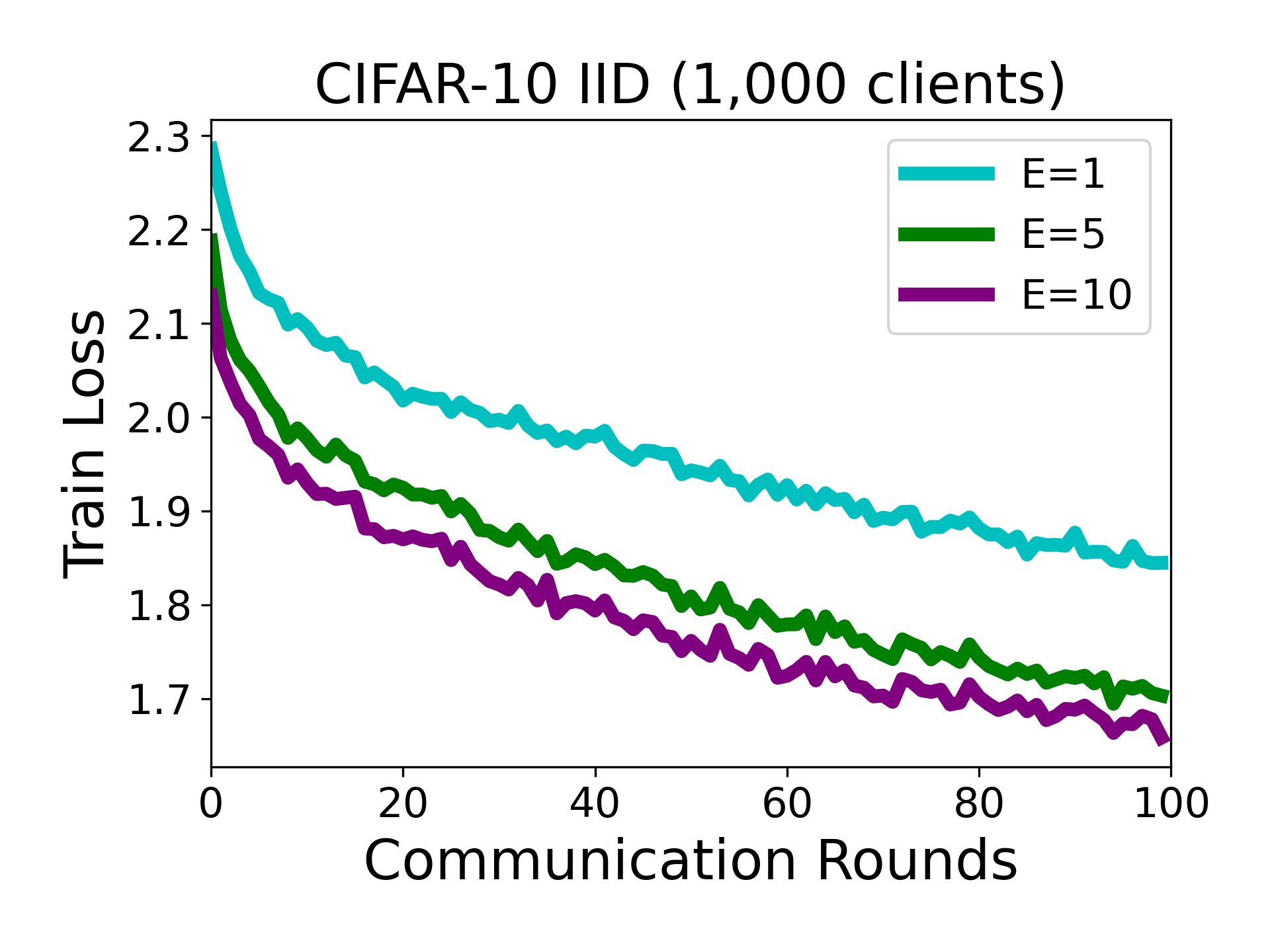
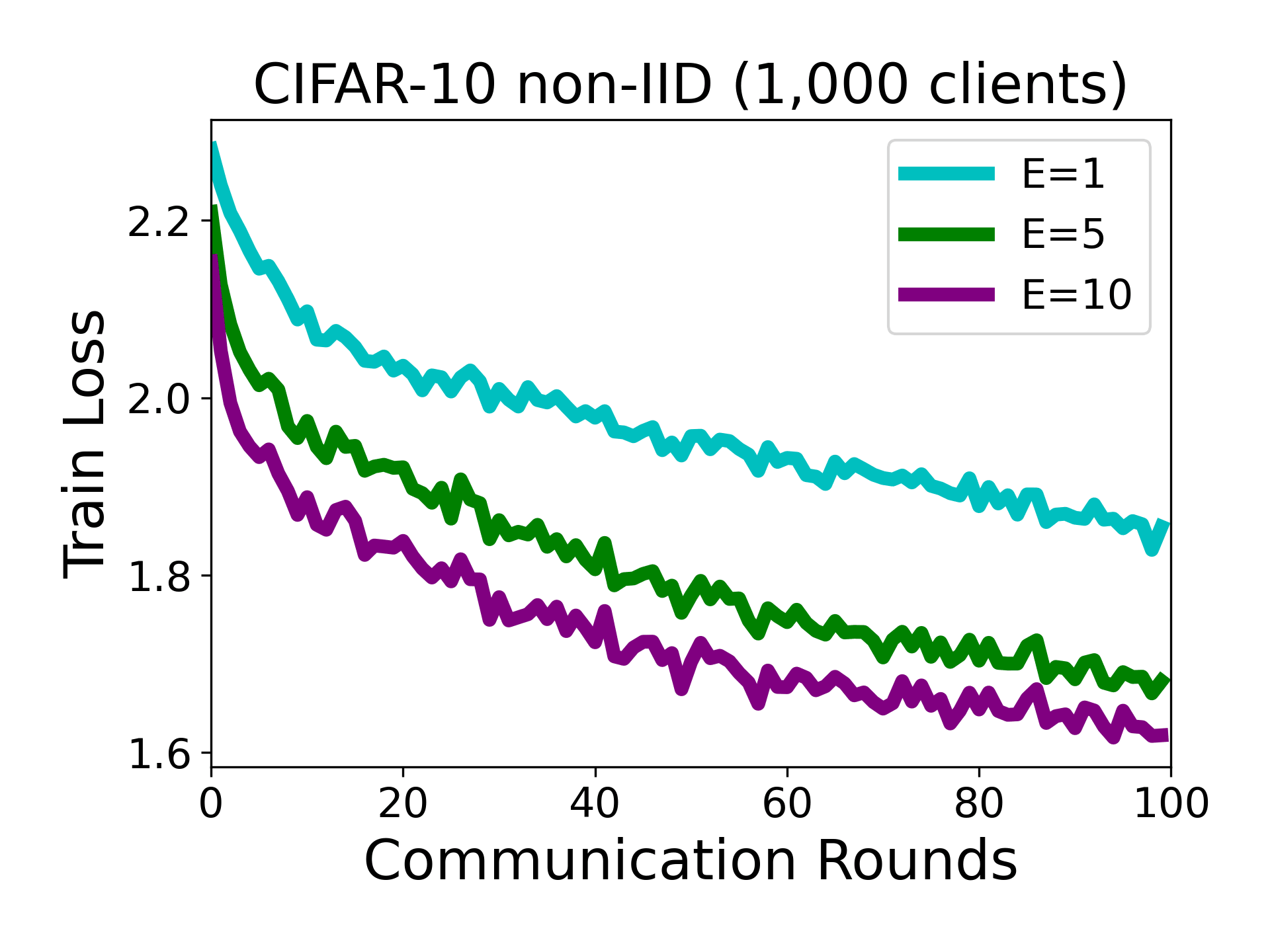
Figure 7: Performance boost with increased local epoch number $E$. Convergence of FedADMM is always ensured even with fixed learning rate and increasing amount of local training.

Increasing Local Work. We investigate how the local epoch number $E$ (capturing the amount of local training) affects the performance of FedADMM. Table IV and Fig. 7 indicate that a more accurate global model can be obtained by increasing the amount of local training. This is in accord with our theoretical analysis (Theorem 1): the fact that the local subproblems are cast as strongly convex guarantees that the larger the local workload, the smaller the $\varepsilon_{i}$ in (6), and thus the better the convergence.

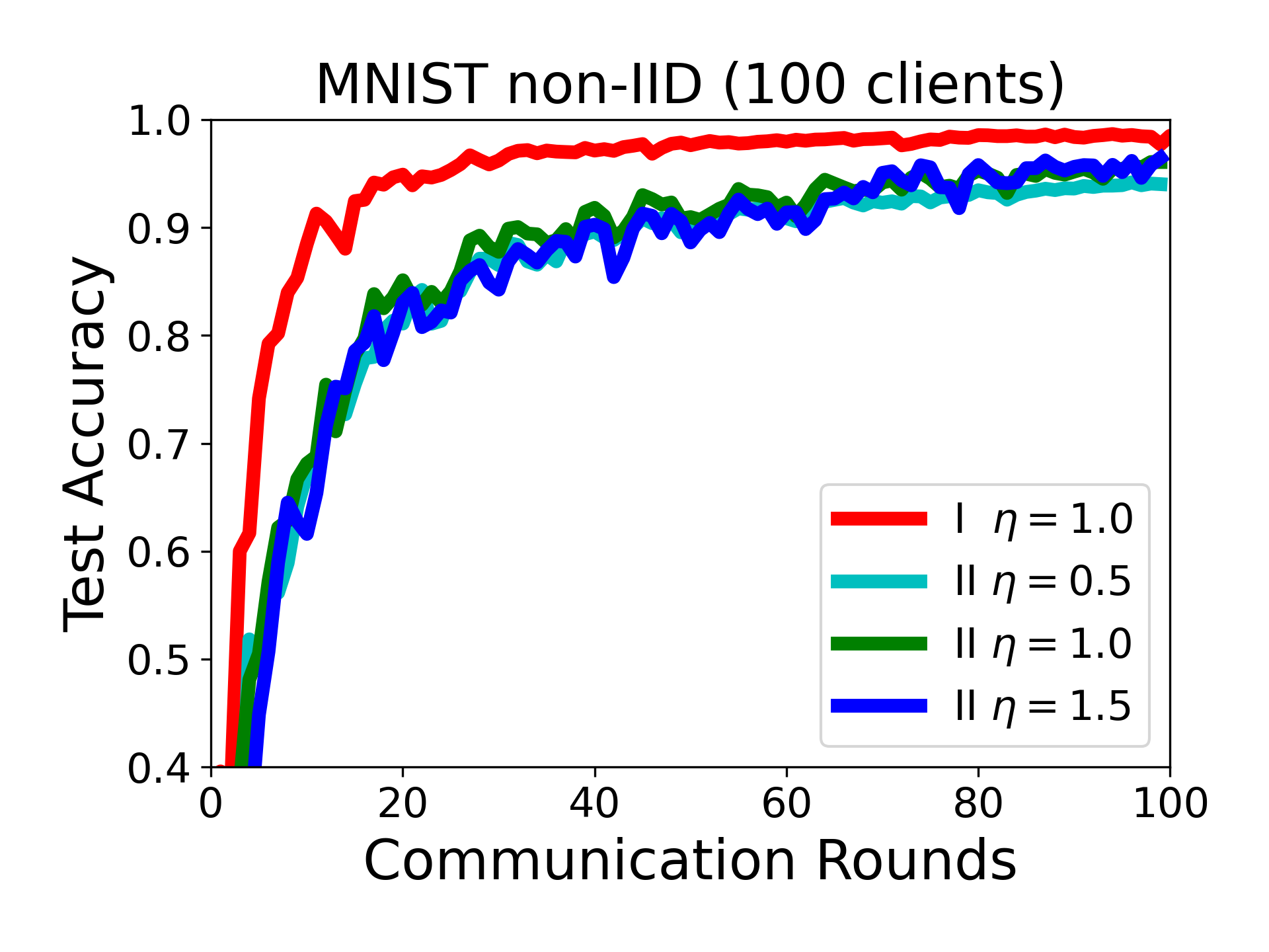
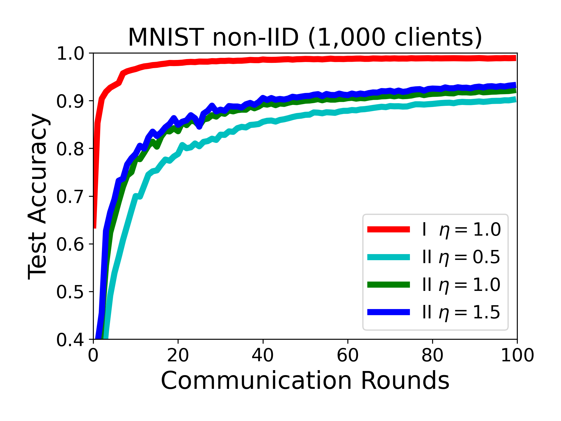
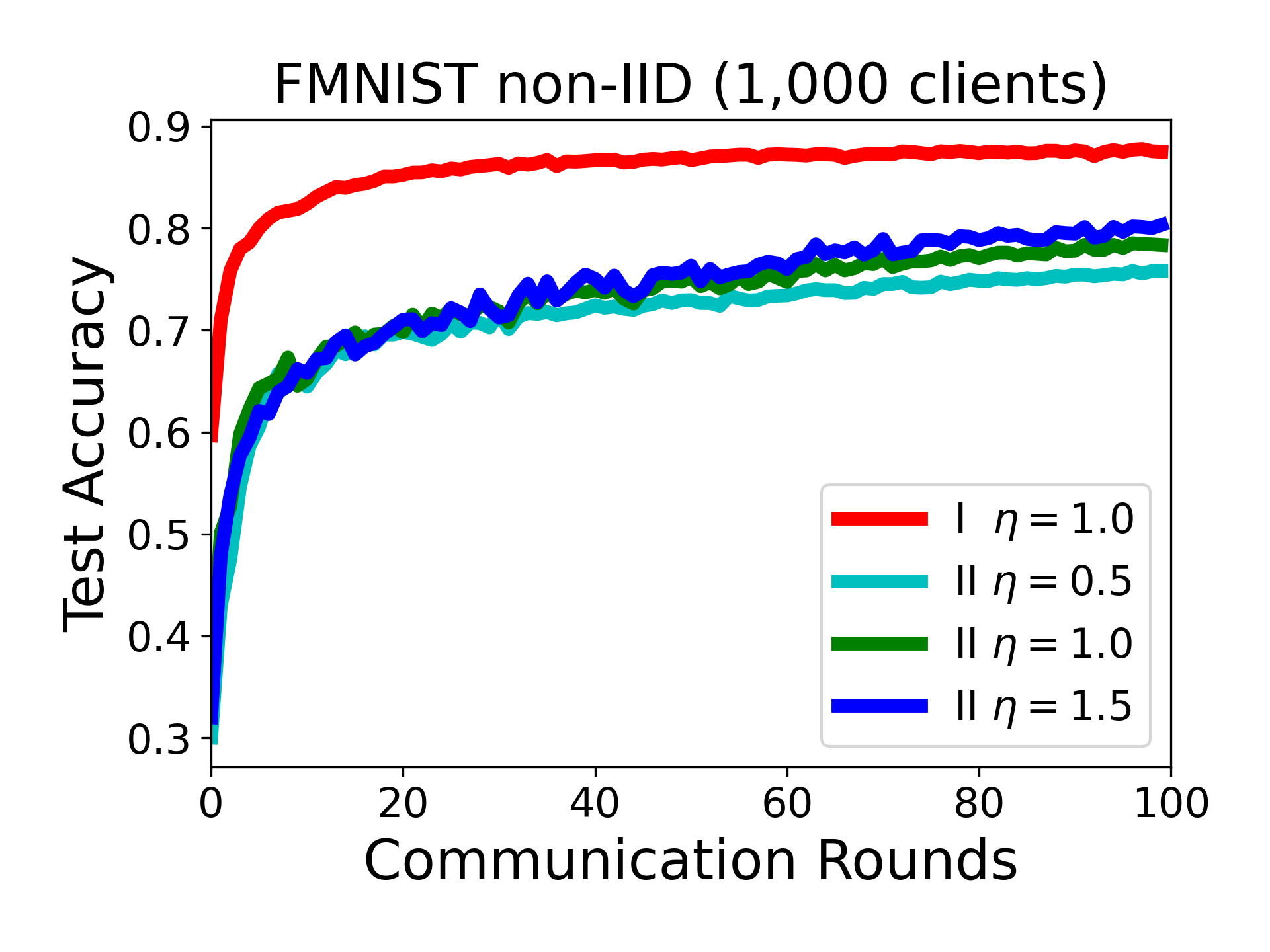
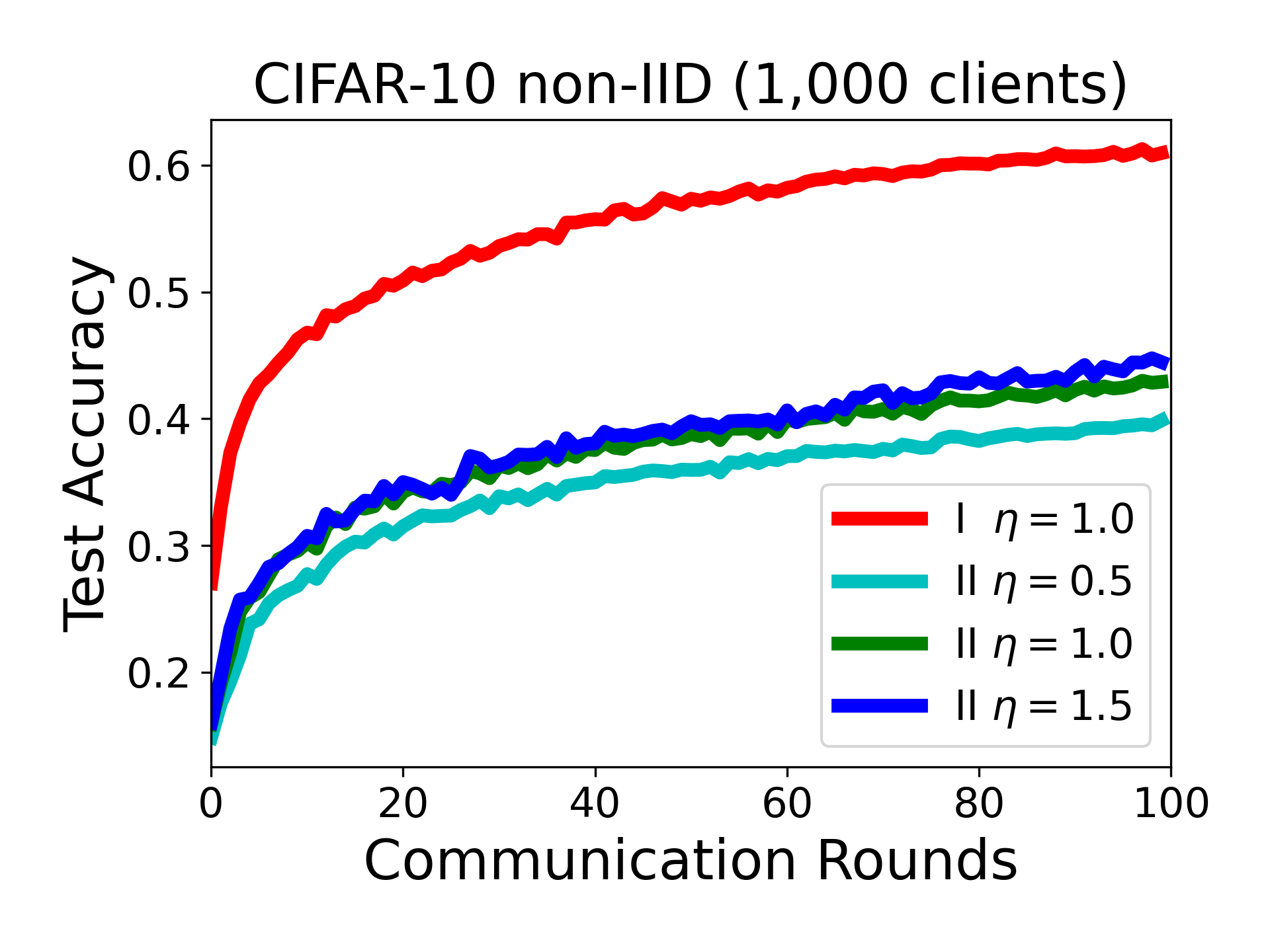
Figure 8: Different choices on local training initialization for FedADMM: I stands for initializing with the local model $w_{i}^{t}$, and II stands for initializing with the global model $\theta^{t}$ (over different server step sizes). Warm starting local training with the local model $w_{i}^{t}$ yields superior results in all cases.

TABLE V: Number of communication rounds to reach a prescribed accuracy (80% for FMNIST, 97% for MNIST). We use fixed $\rho=0.01$ for FedADMM while varying $\rho$ for FedProx. Note that different values of $\rho$ give drastically different results for of FedProx, while FedADMM is consistently superior with constant $\rho$.

		200 clients		500 clients
Dataset	$\rho$	IID	non-IID	IID	non-IID
MNIST	FedADMM ($0.01$)	3	29	5	14
	FedProx ($0.01$)	100+	100+	47	82
	FedProx (0.1)	25	83	59	100+
	FedProx (1)	81	100+	100+	100+
FMNIST	FedADMM ($0.01$)	2	13	2	9
	FedProx (0.01)	5	34	11	45
	FedProx (0.1)	7	45	13	54
	FedProx (1)	43	100+	44	100+

Local Initialization. We further study the performance of FedADMM by investigating the impact of different initialization for the local training subproblems at selected clients. As shown in Fig. 8, using client model parameters $w_{i}^{t}$ as a warm start for the local SGD demonstrates significant advantages compared to using the global model $\theta^{t}$. This provides additional motivation for clients to store their local model $w_{i}$ as compared to using the global model $\theta$ as the starting point for local training.

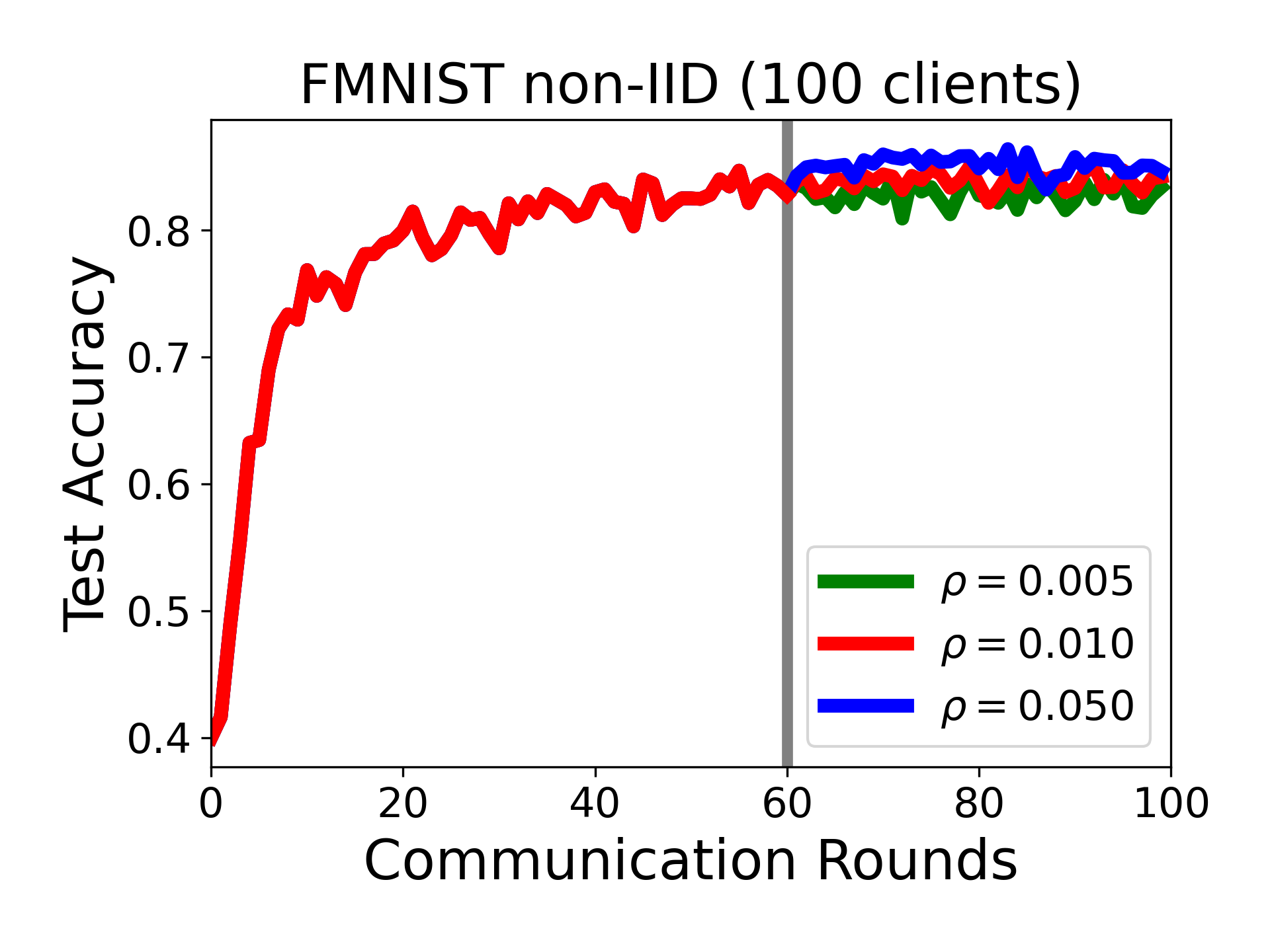
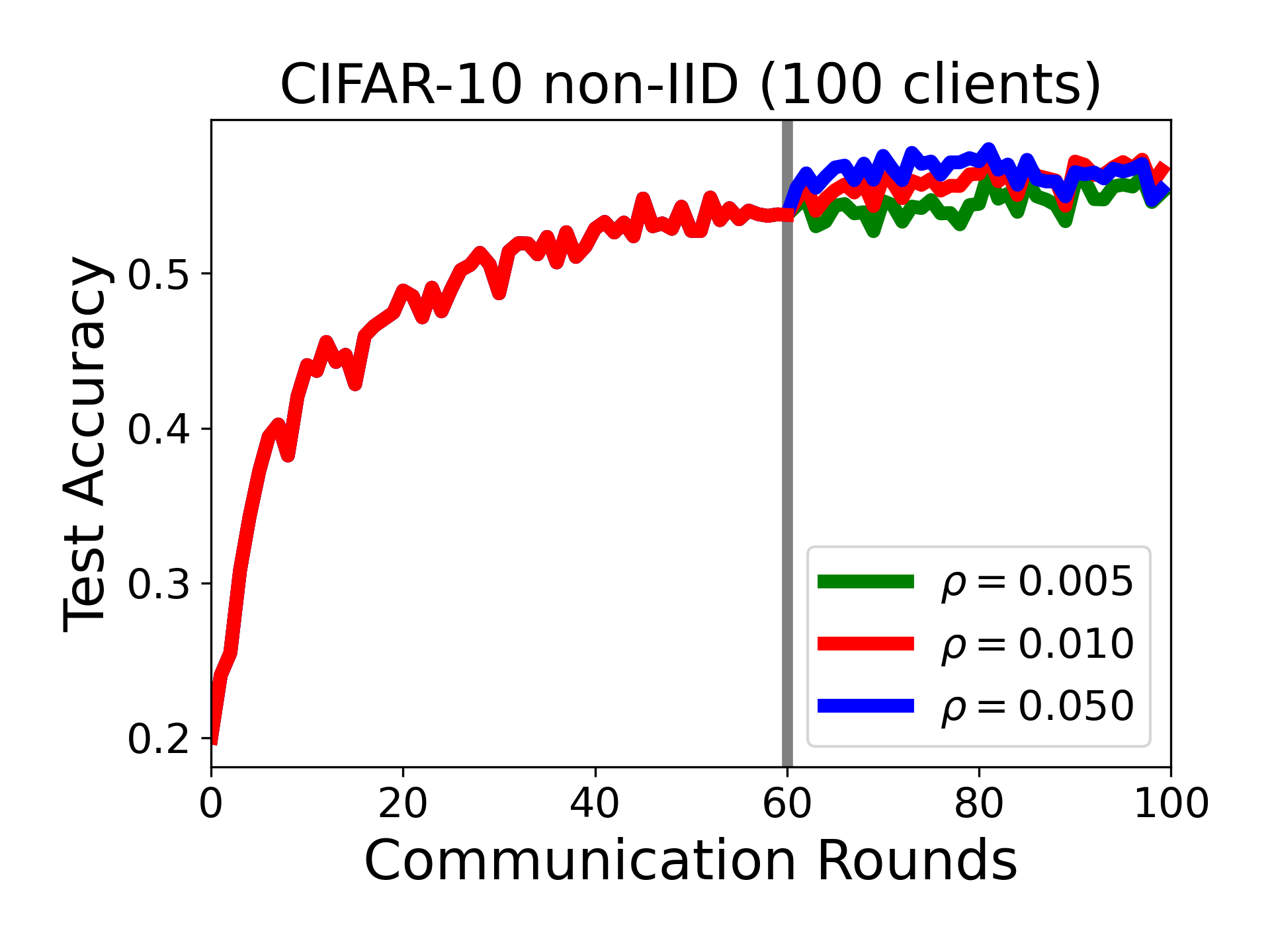
Figure 9: Performance comparison with different value of proximal hyperparameter $\rho$ in FedADMM. The vertical line indicates the point when $\rho$ is changed.

Proximal Parameter $\rho$. To counter client drift in non-IID data distributions, FedADMM and FedProx both use a quadratic proximal term for the local training problem. The proximal coefficient $\rho$ in FedProx has to be carefully tuned to achieve competitive performance across different settings [8], [9]. Such tuning is dependent on system sizes and data distributions, as we also demonstrate in Table V. Note that the best $\rho$ value (0.01) for FedProx in the FMNIST dataset gives the worst performance for MNIST in the 200-client setting. Moreover, the performance of FedProx with respect to $\rho$ is not monotone, which makes tuning even more challenging. On the other hand, FedADMM dominates all tested instances of FedProx with fixed $\rho=0.01$. This is also supported by our theoretical analysis (Theorem 1 and Remark 1 supports a constant $\rho$). Additional insights can be gained by a simple dynamic adaptation of $\rho$ for FedADMM in Fig. 9. A smaller value (0.01) at initial stages of training allows efficient incorporation of local data when the global model is not informed, while an increase of $\rho$ at later stages reduces discrepancies between client models and the global model.

TABLE VI: Statistics of imbalanced datasets.

Dataset	Clients	Samples	Mean	Stdev
FMNIST	200	60,000	300	171.03
CIFAR-10	200	50,000	250	142.52

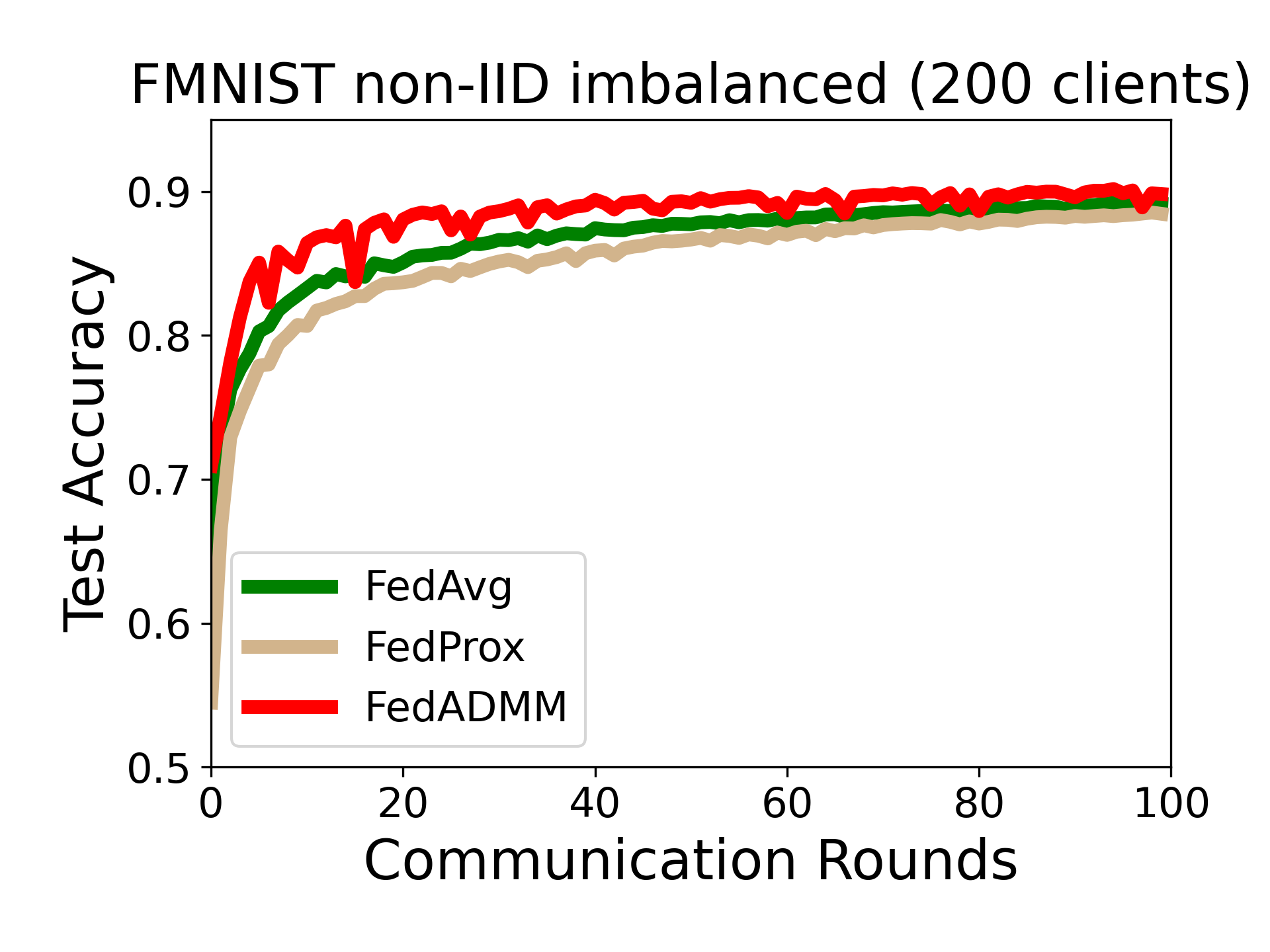
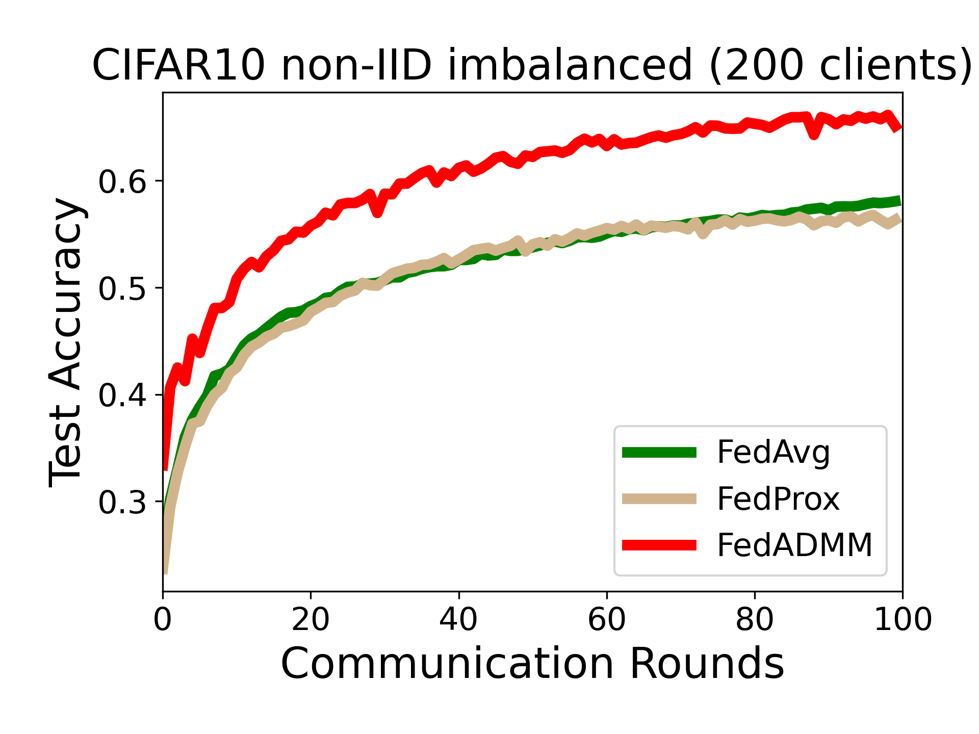
Figure 10: FedADMM achieves the best performance over baseline algorithms for imbalanced datasets ($E=10$, $B=50$).

Imbalanced Data Volumes. We explore the more realistic scenario that clients hold different data volumes. In this setting, we first sort the training data points by labels, then divide the training data into $10,000$ shards, each with 5 data points for CIFAR-10 and 6 data points for FMNIST, respectively. We divide 200 clients evenly into 100 groups. Each member of the group is assigned with a number of shards that equals the group index, except for the last group that collects the remaining data. The setting is summarized in Table VI. Fig. 10 shows that FedADMM achieves higher accuracy than other baselines, especially in the CIFAR-10 dataset.

VI Conclusion

FedADMM is a new federated learning method that handles both statistical and system heterogeneity, without inducing extra communication costs per round. By storing an extra dual variable at each client, a significant speedup over the state-of-the-art is achieved which translates to substantial communication savings. Moreover, FedADMM features automatic adaptation to statistical variations within the system without the need for hyperparameter tuning. Such adaptation safeguards against client drift that causes FedAvg to diverge. We have established an optimal convergence rate (which matches the problem complexity lower bound), with no assumptions on data dissimilarity or gradient boundedness. The analytical results are corroborated by extensive experiments that reveal that FedADMM is well-suited for FL applications with large system sizes and heterogeneous data distributions.

VII Full proof

In this section, we present the full proof of our theoretical results. Our proof of convergence is inspired by [27] but differs in the following aspects allusive to our specific design: (i) the server updates at each round; (ii) the local training problems are solved inexactly with the level of inexactness captured by the local parameter $\varepsilon_{i}$ as in (6); (iii) an additional step size $\eta$ for server aggregation is included. For ease of exposition, we fix $\eta=\absolutevalue{S^{t}}/m$ in the analysis and stack variables as follows: $w^{t}=[(w_{1}^{t})^{\top},\dots,(w_{m}^{t})^{\top}]^{\top},y^{t}=[(y_{1}^{t})^{\top},\dots,(y_{m}^{t})^{\top}]^{\top}\in\mathbb{R}^{md}$. We define the virtual dual update as follows:

$$\norm{\nabla_{w_{i}}\mathcal{L}_{i}(\widehat{w}_{i}^{t+1},y_{i}^{t},\theta^{t})}^{2}\leq\varepsilon_{i},$$ (11)

$$\widehat{y}_{i}^{t+1}=y_{i}^{t}+\rho(\widehat{w}_{i}^{t+1}-\theta^{t}).$$ (12)

In other words, the virtual update for client $i$ is the value for $(w_{i}^{t+1},y_{i}^{t+1})$ if it participates in the current round, i.e., if $i\in S^{t}$, $w_{i}^{t+1}=\widehat{w}_{i}^{t+1}$ and $y_{i}^{t+1}=\widehat{y}_{i}^{t+1}$. As a consequence, we have:

$$\mathbb{E}^{t}[w_{i}^{t+1}-w_{i}^{t}]=p_{i}(\widehat{w}_{i}^{t+1}-w_{i}^{t}),$$

where $\mathbb{E}^{t}[\cdot]$ denotes the conditional expectation at step $t$, and $p_{i}$ denotes the probability of client $i$ being active. We proceed to bound $\norm{y_{i}^{t+1}-y_{i}^{t}}$ in the following lemma.

Lemma 1: Recall assumption 1 and the local accuracy $\varepsilon_{i}$ in (6). The consecutive difference between dual variables can be bounded as follows:

$$\norm{\widehat{y}_{i}^{t+1}-y_{i}^{t}}^{2}\leq 8\varepsilon_{i}+2L^{2}\norm{\widehat{w}_{i}^{t+1}-w_{i}^{t}}^{2},$$ (13)

$$\norm{y_{i}^{t+1}-y_{i}^{t}}^{2}\leq 8\varepsilon_{i}+2L^{2}\norm{w_{i}^{t+1}-w_{i}^{t}}^{2}.$$ (14)

Proof: We first prove (13) by defining the local error term as

$$e_{i}^{t+1} =\nabla_{w_{i}}\mathcal{L}_{i}(\widehat{w}_{i}^{t+1},y_{i}^{t},\theta^{t})$$

$$=\nabla f_{i}(\widehat{w}_{i}^{t+1})+y_{i}^{t}+\rho(\widehat{w}_{i}^{t+1}-\theta^{t})$$

$$=\nabla f_{i}(\widehat{w}_{i}^{t+1})+\widehat{y}_{i}^{t+1},$$ (15)

where the last equality holds from the definition of virtual update rule (12). Note that $\norm{e_{i}^{t+1}}=\norm{\nabla_{w_{i}}\mathcal{L}_{i}(\widehat{w}_{i}^{t+1},y_{i}^{t},\theta^{t})}\leq\sqrt{\varepsilon_{i}}$. By rearranging and taking the difference,

$$\norm{\widehat{y}_{i}^{t+1}-y_{i}^{t}} =\norm{e_{i}^{t+1}-e_{i}^{t}+\nabla f_{i}(w_{i}^{t})-\nabla f_{i}(\widehat{w}_{i}^{t+1})}$$

$$\leq\norm{e_{i}^{t+1}}+\norm{e_{i}^{t}}+\norm{\nabla f_{i}(w_{i}^{t})-\nabla f_{i}(\widehat{w}_{i}^{t+1})}$$

$$\leq 2\sqrt{\varepsilon_{i}}+L\norm{\widehat{w}_{i}^{t+1}-w_{i}^{t}}.$$

Using the inequality $\norm{\sum_{i=1}^{m}a_{i}}^{2}\leq m\sum_{i=1}^{m}\norm{a_{i}}^{2}$, we obtain:

$$\norm{\widehat{y}_{i}^{t+1}-y_{i}^{t}}^{2}\leq 8\varepsilon_{i}+2L^{2}\norm{\widehat{w}_{i}^{t+1}-w_{i}^{t}}^{2},$$

which is the desired. We note that (13) holds for all $i\in[m]$ and proceed to show (14) as follows. For $i\in S^{t}$, $y_{i}^{t+1}=\widehat{y}_{i}^{t+1}$, $w^{t+1}_{i}=\widehat{w}^{t+1}_{i}$, and therefore (14) reduces to (13). For $i\notin S^{t}$, $w_{i}^{t+1}=w_{i}^{t}$, $y_{i}^{t+1}=y_{i}^{t}$, and therefore (14) trivially holds. $\blacksquare$

We denote the aggregated Lagrangian as $\mathcal{L}(w^{t},y^{t},\theta^{t})=\sum_{i=1}^{m}\mathcal{L}_{i}(w_{i}^{t},y_{i}^{t},\theta^{t})$ and proceed to bound its change after one round.

Lemma 2: The aggregated Lagrangian $\mathcal{L}^{t}\equiv\mathcal{L}(w^{t},y^{t},\theta^{t})$ iterates satisfy:

$$\mathcal{L}^{t+1}-\mathcal{L}^{t}\leq\sum_{i\in S^{t}}\Bigg{(}\bigg{(}\tfrac{2L-\rho}{2}+\tfrac{2L^{2}}{\rho}\bigg{)}\norm{w_{i}^{t+1}-w_{i}^{t}}^{2}$$

$$+\tfrac{\varepsilon_{i}}{2L}+\tfrac{8\varepsilon_{i}}{\rho}\Bigg{)}-\tfrac{m\rho}{2}\norm{\theta^{t+1}-\theta^{t}}^{2}.$$ (16)

Proof: We decompose the difference into three parts:

$$\mathcal{L}^{t+1}-\mathcal{L}^{t}=\mathcal{L}(w^{t+1},y^{t+1},\theta^{t+1})-\mathcal{L}(w^{t+1},y^{t+1},\theta^{t})$$

$$+\mathcal{L}(w^{t+1},y^{t+1},\theta^{t})-\mathcal{L}(w^{t+1},y^{t},\theta^{t})$$

$$+\mathcal{L}(w^{t+1},y^{t},\theta^{t})-\mathcal{L}(w^{t},y^{t},\theta^{t}).$$ (17)

The three difference terms in (17) correspond to the $\theta^{t+1}$-update, $y^{t+1}$-update, and $w^{t+1}$-update, respectively. We proceed to bound each term separately. Note that $\mathcal{L}(\cdot)$ is strongly convex with respect to $\theta$ with parameter $m\rho$. Therefore,

$$\mathcal{L}(w^{t+1},y^{t+1},\theta^{t})\geq\mathcal{L}^{t+1}+\langle\nabla_{\theta}\mathcal{L}^{t+1},\theta^{t}-\theta^{t+1}\rangle$$

$$+\tfrac{m\rho}{2}\norm{\theta^{t+1}-\theta^{t}}^{2}.$$ (18)

By definition,

$$\nabla_{\theta}\mathcal{L}^{t+1}=\rho\left(m\theta^{t+1}-\sum_{i=1}^{m}(w_{i}^{t+1}+\tfrac{1}{\rho}y_{i}^{t+1})\right).$$ (19)

When the server step size is chosen as $\eta=\absolutevalue{S^{t}}/m$, we have

$$\theta^{t+1} =\theta^{t}+\tfrac{1}{m}\sum_{i\in S^{t}}\left(w_{i}^{t+1}+\tfrac{1}{\rho}y_{i}^{t+1}-(w_{i}^{t}+\tfrac{1}{\rho}y_{i}^{t})\right)$$

$$=\theta^{t}+\tfrac{1}{m}\sum_{i=1}^{m}(u_{i}^{t+1}-u_{i}^{t}),$$

where we have defined the augmented model $u_{i}^{t}=w_{i}^{t}+\tfrac{1}{\rho}y_{i}^{t}$ and used the fact that for $i\notin S^{t}$, $u_{i}^{t+1}-u_{i}^{t}=0$. After telescoping, we obtain

$$\theta^{t+1}=\theta^{0}+\tfrac{1}{m}\sum_{i=1}^{m}(u_{i}^{t+1}-u_{i}^{0}).$$

From our initialization, $w_{i}^{0}=\theta^{0}$ and $y_{i}^{0}=0$, it follows that $\tfrac{1}{m}\sum_{i=1}^{m}u_{i}^{0}=\theta^{0}$. Therefore, $\theta^{t+1}=\tfrac{1}{m}\sum_{i=1}^{m}u_{i}^{t+1}$. Using this fact along with (19), we obtain

$$\nabla_{\theta}\mathcal{L}^{t+1}=\rho\sum_{i=1}^{m}\left(u_{i}^{t+1}-(w_{i}^{t+1}+\tfrac{1}{\rho}y_{i}^{t+1})\right)=0,$$ (20)

where we used the definition $u_{i}^{t+1}=w_{i}^{t+1}+\tfrac{1}{\rho}y_{i}^{t+1}$. Therefore, we can rewrite (18) as

$$\mathcal{L}^{t+1}-\mathcal{L}(w^{t+1},y^{t+1},\theta^{t})\leq-\tfrac{m\rho}{2}\norm{\theta^{t+1}-\theta^{t}}^{2},$$ (21)

which is the bound for the first difference term in (17). By definition, the second difference term in (17) can be expressed as:

$$\mathcal{L}(w^{t+1},y^{t+1},\theta^{t})-\mathcal{L}(w^{t+1},y^{t},\theta^{t})\qquad$$

$$=\sum_{i\in S^{t}}\langle y_{i}^{t+1}-y_{i}^{t},w_{i}^{t+1}-\theta^{t}\rangle$$

$$=\sum_{i\in S^{t}}\tfrac{1}{\rho}\norm{y_{i}^{t+1}-y_{i}^{t}}^{2},$$

where the last equality follows from (12) and the fact that for $i\in S^{t}$, $y_{i}^{t+1}=\widehat{y}_{i}^{t+1}$, $w_{i}^{t+1}=\widehat{w}_{i}^{t+1}$. Using Lemma 1, we obtain

$$\mathcal{L}(w^{t+1},y^{t+1},\theta^{t})-\mathcal{L}(w^{t+1},y^{t},\theta^{t})$$

$$\leq\sum_{i\in S^{t}}\bigg{(}\tfrac{8\varepsilon_{i}}{\rho}+\tfrac{2L^{2}}{\rho}\norm{w_{i}^{t+1}-w_{i}^{t}}^{2}\bigg{)},$$ (22)

which is the bound for the second difference term in (17). For the third difference term, we first note that $-\nabla f_{i}(\cdot)$ is Lipschitz as well. Therefore, the following holds:

$$-f_{i}(w_{i}^{t})\leq-f_{i}(w_{i}^{t+1})+\langle-\nabla f_{i}(w_{i}^{t+1}),w_{i}^{t}-w_{i}^{t+1}\rangle$$

$$+\tfrac{L}{2}\norm{w_{i}^{t+1}-w_{i}^{t}}^{2},$$ (23)

and $\forall\,i\in S^{t}$:

$$\mathcal{L}_{i}(w_{i}^{t+1},y_{i}^{t},\theta^{t})-\mathcal{L}_{i}(w_{i}^{t},y_{i}^{t},\theta^{t})$$

$$=f_{i}(w_{i}^{t+1})-f_{i}(w^{t}_{i})+\langle y_{i}^{t},w_{i}^{t+1}-w_{i}^{t}\rangle$$

$$\quad+\tfrac{\rho}{2}\left(\norm{w_{i}^{t+1}-\theta^{t}}^{2}-\norm{w_{i}^{t}-\theta^{t}}^{2}\right)$$

$$\underset{(\text{i})}{\leq}\langle\nabla f_{i}(w_{i}^{t+1}),w_{i}^{t+1}-w_{i}^{t}\rangle+\tfrac{L}{2}\norm{w_{i}^{t+1}-w_{i}^{t}}^{2}$$

$$\quad+\langle y_{i}^{t},w_{i}^{t+1}-w_{i}^{t}\rangle+\tfrac{\rho}{2}\langle w_{i}^{t+1}+w_{i}^{t}-2\theta^{t},w_{i}^{t+1}-w_{i}^{t}\rangle$$

$$\underset{(\text{ii})}{=}\langle\nabla f_{i}(w_{i}^{t+1})+y_{i}^{t}+\tfrac{\rho}{2}\cdot 2(w_{i}^{t+1}-\theta^{t}),w_{i}^{t+1}-w_{i}^{t}\rangle$$

$$\quad+\tfrac{L}{2}\norm{w_{i}^{t+1}-w_{i}^{t}}^{2}+\tfrac{\rho}{2}\langle w_{i}^{t}-w_{i}^{t+1},w_{i}^{t+1}-w_{i}^{t}\rangle$$

$$\underset{(\text{iii})}{\leq}\tfrac{1}{2L}\norm{\nabla f_{i}(w_{i}^{t+1})+y_{i}^{t+1}}^{2}+\tfrac{2L-\rho}{2}\norm{w_{i}^{t+1}-w_{i}^{t}}^{2}$$

$$\underset{(\text{iv})}{\leq}\tfrac{\varepsilon_{i}}{2L}+\tfrac{2L-\rho}{2}\norm{w_{i}^{t+1}-w_{i}^{t}}^{2}.$$ (24)

In (24): (i) follows from (23) and the identity $\norm{a}^{2}-\norm{b}^{2}=(a+b)^{\top}(a-b)$; (ii) follows from splitting $w_{i}^{t+1}+w_{i}^{t}-2\theta^{t}=2(w_{i}^{t+1}-\theta^{t})+w_{i}^{t}-w_{i}^{t+1}$; (iii) follows from the dual update: $y_{i}^{t+1}=y_{i}^{t}+\rho(w_{i}^{t+1}-\theta^{t})$ and the identity $a^{\top}b\leq\tfrac{1}{2L}\norm{a}^{2}+\tfrac{L}{2}\norm{b}^{2}$; (iv) follows from (15) and (11). Therefore, the third difference term in (17) can be bounded as:

$$\mathcal{L}(w^{t+1},y^{t},\theta^{t})-\mathcal{L}^{t}\leq\sum_{i\in S^{t}}\tfrac{2L-\rho}{2}\norm{w_{i}^{t+1}-w_{i}^{t}}^{2}+\sum_{i\in S^{t}}\tfrac{\varepsilon_{i}}{2L}.$$ (25)

After combining (21), (22) and (25), we obtain the desired. $\blacksquare$

We proceed to establish a lower bound for the augmented Lagrangian in the following lemma.

Lemma 3. Recall the lower bound $\sum_{i=1}^{m}f_{i}(w)\geq f^{\star}$ in assumption 2. For $t\geq 0$, the augmented Lagrangian is lower bounded as $\mathcal{L}^{t+1}\geq f^{\star}-\tfrac{1}{2L}\sum_{i=1}^{m}\varepsilon_{i}$ by selecting $\rho\geq 2L$.

Proof: By definition,

$$\mathcal{L}^{t+1} =\sum_{i=1}^{m}\bigg{(}f_{i}(w_{i}^{t+1})+\langle y_{i}^{t+1},w_{i}^{t+1}-\theta^{t+1}\rangle$$

$$\quad+\tfrac{\rho}{2}\norm{w_{i}^{t+1}-\theta^{t+1}}^{2}\bigg{)}$$

$$\underset{(\text{i})}{=}\sum_{i=1}^{m}\bigg{(}f_{i}(w_{i}^{t+1})+\langle\nabla f_{i}(w_{i}^{t+1}),\theta^{t+1}-w_{i}^{t+1}\rangle$$

$$\quad+\tfrac{\rho}{2}\norm{w_{i}^{t+1}-\theta^{t+1}}^{2}+\langle e_{i}^{t+1},w_{i}^{t+1}-\theta^{t+1}\rangle\bigg{)}$$

$$\underset{(\text{ii})}{\geq}\sum_{i=1}^{m}\bigg{(}f_{i}(\theta^{t+1})+\tfrac{\rho-2L}{2}\norm{w_{i}^{t+1}-\theta^{t+1}}^{2}-\tfrac{1}{2L}\varepsilon_{i}\bigg{)}$$

$$\geq\sum_{i=1}^{m}f_{i}(\theta^{t+1})-\tfrac{1}{2L}\sum_{i=1}^{m}\varepsilon_{i}\geq f^{\star}-\tfrac{1}{2L}\sum_{i=1}^{m}\varepsilon_{i}.$$ (26)

To show equality (i) holds, it suffices to show: $\forall\,i$, $y_{i}^{t+1}=e_{i}^{t+1}-\nabla f_{i}(w_{i}^{t+1})$. This holds for $i\in S^{t}$ by (15) and the fact that $\widehat{w}_{i}^{t+1}=w_{i}^{t+1},\widehat{y}_{i}^{t+1}=y_{i}^{t+1}$. For $i\notin S^{t}$, $w_{i}^{t+1}=w_{i}^{t}=w_{i}^{t_{i}+1}$, where we denote $t_{i}$ as the most recent time step when client $i$ is selected before step $t$. Therefore, for $i\notin S^{t}$, $y_{i}^{t+1}=y_{i}^{t}=y_{i}^{t_{i}+1}=e_{i}^{t_{i}+1}-\nabla f_{i}(w_{i}^{t_{i}+1})=e_{i}^{t+1}-\nabla f_{i}(w_{i}^{t+1})$. The inequality (ii) follows from a consequence of assumption 1, the identity $a^{\top}b\geq-\tfrac{L}{2}\norm{a}^{2}-\tfrac{1}{2L}\norm{b}^{2}$, and $\norm{e_{i}^{t+1}}^{2}\leq\varepsilon_{i}$. $\blacksquare$

Recall the non-negative function $V^{t}\equiv V(w^{t},y^{t},\theta^{t})$ defined in (7):

$$V^{t}=\norm{\nabla_{\theta}\mathcal{L}^{t}}^{2}+\sum_{i=1}^{m}\left(\norm{\nabla_{w_{i}}\mathcal{L}^{t}}^{2}+\norm{w_{i}^{t}-\theta^{t}}^{2}\right).$$

We establish the convergence of the FedADMM in the following.

Theorem 1. Let assumptions 1 and 2 hold. Assume each client has a probability of participating at a given round that is lower bounded by a positive constant $p_{\mathrm{min}}>0$. Consider $\eta=\absolutevalue{S^{t}}/m$, and select $\rho>(1+\sqrt{5})L$, then the following holds:

$$\tfrac{1}{mT}\sum_{t=0}^{T-1}\mathbb{E}[V^{t}]\leq\tfrac{1}{mT}\tfrac{c_{2}}{c_{1}}\left(\mathcal{L}^{0}-f^{\star}+\tfrac{m}{2L}\varepsilon_{\mathrm{max}}\right)+c_{3}\varepsilon_{\mathrm{max}},$$ (8)

where $\varepsilon_{\mathrm{max}}=\max_{i}\,\varepsilon_{i}$, $c_{1}=p_{\mathrm{min}}\left(\tfrac{\rho-2L}{2}-\tfrac{2L^{2}}{\rho}\right)$, $c_{2}=3(L^{2}+\rho^{2})+2(1+\tfrac{2L^{2}}{\rho^{2}})$, and $c_{3}=3+\tfrac{16}{\rho^{2}}+\tfrac{c_{2}}{c_{1}}\cdot\tfrac{\rho+16L}{2L\rho}$.

Proof: By definition, the following holds:

$$\norm{\nabla_{w_{i}}\mathcal{L}_{i}^{t}}^{2}=\norm{\nabla f_{i}(w_{i}^{t})+y_{i}^{t}+\rho(w_{i}^{t}-\theta^{t})}^{2}.$$

Recall (15) where

$$e_{i}^{t+1}=\nabla f_{i}(\widehat{w}_{i}^{t+1})+y_{i}^{t}+\rho(\widehat{w}_{i}^{t+1}-\theta^{t}).$$

Therefore, we obtain

$$\norm{\nabla_{w_{i}}\mathcal{L}_{i}^{t}} =\norm{\nabla f_{i}(w_{i}^{t})+y_{i}^{t}+\rho(w_{i}^{t}-\theta^{t})}$$

$$=\bigg{|}\bigg{|}\nabla f_{i}(w_{i}^{t})+y_{i}^{t}+\rho(w_{i}^{t}-\theta^{t})$$

$$\quad-\bigg{(}\nabla f_{i}(\widehat{w}_{i}^{t+1})+y_{i}^{t}+\rho(\widehat{w}_{i}^{t+1}-\theta^{t})\bigg{)}+e_{i}^{t+1}\bigg{|}\bigg{|}$$

$$= \norm{\nabla f_{i}(w_{i}^{t})-\nabla f_{i}(\widehat{w}_{i}^{t+1})+\rho(w_{i}^{t}-\widehat{w}_{i}^{t+1})+e_{i}^{t+1}}$$

$$\leq \norm{\nabla f_{i}(w_{i}^{t})-\nabla f_{i}(\widehat{w}_{i}^{t+1})}+\rho\norm{w_{i}^{t}-\widehat{w}_{i}^{t+1}}+\norm{e_{i}^{t+1}}$$

Using assumption 1, and the accuracy for inexact primal updates, we obtain

$$\norm{\nabla_{w_{i}}\mathcal{L}_{i}^{t}}^{2}\leq 3\bigg{(}\left(L^{2}+\rho^{2}\right)\norm{\widehat{w}_{i}^{t+1}-w_{i}^{t}}^{2}+\varepsilon_{i}\bigg{)}.$$

Therefore, it holds that

$$\sum_{i=1}^{m}\norm{\nabla_{w_{i}}\mathcal{L}_{i}^{t}}^{2}\leq 3\sum_{i=1}^{m}\left(\bigg{(}L^{2}+\rho^{2}\bigg{)}\norm{\widehat{w}^{t+1}_{i}-w_{i}^{t}}^{2}+\varepsilon_{i}\right).$$ (27)

Moreover,

$$\sum_{i=1}^{m}\norm{w_{i}^{t}-\theta^{t}}^{2} =\sum_{i=1}^{m}\norm{w_{i}^{t}-\widehat{w}_{i}^{t+1}+\widehat{w}_{i}^{t+1}-\theta^{t}}^{2}$$

$$\leq\sum_{i=1}^{m}2\bigg{(}\norm{\widehat{w}_{i}^{t+1}-w_{i}^{t}}^{2}+\norm{\widehat{w}_{i}^{t+1}-\theta^{t}}^{2}\bigg{)}.$$

From the virtual update for $\widehat{y}_{i}^{t+1}$ in (12),

$$\norm{\widehat{w}_{i}^{t+1}-\theta^{t}}^{2}=\tfrac{1}{\rho^{2}}\norm{\widehat{y}_{i}^{t+1}-y_{i}^{t}}^{2}.$$ (28)

Therefore, we obtain:

$$\sum_{i=1}^{m}\norm{w_{i}^{t}-\theta^{t}}^{2}\leq\sum_{i=1}^{m}2\bigg{(}\norm{\widehat{w}_{i}^{t+1}-w_{i}^{t}}^{2}+\tfrac{1}{\rho^{2}}\norm{\widehat{y}_{i}^{t+1}-y_{i}^{t}}^{2}\bigg{)}$$

$$\leq 2\sum_{i=1}^{m}\left(\bigg{(}1+\tfrac{2L^{2}}{\rho^{2}}\bigg{)}\norm{\widehat{w}_{i}^{t+1}-w_{i}^{t}}^{2}+\tfrac{8\varepsilon_{i}}{\rho^{2}}\right),$$ (29)

where the last inequality follows from Lemma 1. From (20) we obtain:

$$V^{t} =\underbrace{\norm{\nabla_{\theta}\mathcal{L}^{t}}^{2}}_{\text{ $=0$}}+\sum_{i=1}^{m}\bigg{(}\norm{\nabla_{w_{i}}\mathcal{L}_{i}^{t}}^{2}+\norm{w_{i}^{t}-\theta^{t}}^{2}\bigg{)}$$

$$\underset{(\ref{theorem_comp1})-(\ref{theorem1_comp2})}{\leq}\sum_{i=1}^{m}\bigg{(}3(L^{2}+\rho^{2})+2(1+\tfrac{2L^{2}}{\rho^{2}})\bigg{)}\norm{\widehat{w}_{i}^{t+1}-w_{i}^{t}}^{2}$$

$$\quad+\sum_{i=1}^{m}\bigg{(}3+\tfrac{16}{\rho^{2}}\bigg{)}\varepsilon_{i}$$

$$\leq\sum_{i=1}^{m}c_{2}\norm{\widehat{w}_{i}^{t+1}-w_{i}^{t}}^{2}+\left(3m+\tfrac{16m}{\rho^{2}}\right)\varepsilon_{\mathrm{max}},$$ (30)

where the last inequality follows from the definitions: $\varepsilon_{\mathrm{max}}=\underset{i}{\mathrm{max}}\,\,\varepsilon_{i},c_{2}=3(L^{2}+\rho^{2})+2(1+\tfrac{2L^{2}}{\rho^{2}})$. From Lemma 2, we have $\mathcal{L}^{t+1}-\mathcal{L}^{t}\leq\sum_{i\in S^{t}}\Bigg{(}\bigg{(}\tfrac{2L-\rho}{2}+\tfrac{2L^{2}}{\rho}\bigg{)}\norm{w_{i}^{t+1}-w_{i}^{t}}^{2}+\tfrac{\varepsilon_{i}}{2L}+\tfrac{8\varepsilon_{i}}{\rho}\Bigg{)}-\tfrac{m\rho}{2}\norm{\theta^{t+1}-\theta^{t}}^{2}.$ After taking conditional expectation at step $t$, by using linearity of expectation and rearranging, we obtain:

$$\mathbb{E}^{t}\left[\mathcal{L}^{t}-\mathcal{L}^{t+1}\right]\geq p_{\mathrm{min}}\sum_{i=1}^{m}\left(\tfrac{\rho-2L}{2}-\tfrac{2L^{2}}{\rho}\right)\norm{\widehat{w}_{i}^{t+1}-w_{i}^{t}}^{2}$$

$$-m\left(\tfrac{\varepsilon_{\mathrm{max}}}{2L}+\tfrac{8\varepsilon_{\mathrm{max}}}{\rho}\right)+\tfrac{m\rho}{2}\norm{\overline{\theta}^{t+1}-\theta^{t}}^{2},$$ (31)

where we denote $\mathbb{E}^{t}\left[\theta^{t+1}\right]=\overline{\theta}^{t+1}$ and used Jensen’s inequality: $\mathbb{E}^{t}\left[\norm{\theta^{t+1}-\theta^{t}}^{2}\right]\geq\norm{\mathbb{E}^{t}\left[\theta^{t+1}\right]-\theta^{t}}^{2}=\norm{\overline{\theta}^{t+1}-\theta^{t}}^{2}.$ Defining $c_{1}=p_{\mathrm{min}}(\tfrac{\rho-2L}{2}-\tfrac{2L^{2}}{\rho})$, we rewrite (31) as

$$\mathbb{E}^{t}[\mathcal{L}^{t}-\mathcal{L}^{t+1}]+m\left(\tfrac{\varepsilon_{\mathrm{max}}}{2L}+\tfrac{8\varepsilon_{\mathrm{max}}}{\rho}\right)\geq c_{1}\sum_{i=1}^{m}\norm{\widehat{w}_{i}^{t+1}-w_{i}^{t}}^{2}.$$ (32)

Using (30) and (32) leads to:

$$V^{t}\leq\tfrac{c_{2}}{c_{1}}\mathbb{E}^{t}[\mathcal{L}^{t}-\mathcal{L}^{t+1}]+mc_{3}\varepsilon_{\mathrm{max}},$$ (33)

where $c_{3}=3+\tfrac{16}{\rho^{2}}+\tfrac{c_{2}}{c_{1}}(\tfrac{1}{2L}+\tfrac{8}{\rho})$. Taking expectation on both sides gives

$$\mathbb{E}[V^{t}]\leq\tfrac{c_{2}}{c_{1}}\mathbb{E}[\mathcal{L}^{t}-\mathcal{L}^{t+1}]+mc_{3}\varepsilon_{\mathrm{max}}.$$

After telescoping the above and dividing by $mT$, we obtain:

$$\tfrac{1}{mT}\sum_{t=0}^{T-1}\mathbb{E}\left[V^{t}\right]\leq\tfrac{1}{mT}\tfrac{c_{2}}{c_{1}}\mathbb{E}\left[\mathcal{L}^{0}-\mathcal{L}^{T-1}\right]+c_{3}\varepsilon_{\mathrm{max}}.$$

From Lemma 3, it holds that $\mathbb{E}[\mathcal{L}^{0}-\mathcal{L}^{T-1}]\leq\mathcal{L}^{0}-f^{\star}+\tfrac{m}{2L}\varepsilon_{\mathrm{max}}$. Therefore, the following holds:

$$\tfrac{1}{mT}\sum_{t=0}^{T-1}\mathbb{E}[V^{t}]\leq\tfrac{1}{mT}\tfrac{c_{2}}{c_{1}}\left(\mathcal{L}^{0}-f^{\star}+\tfrac{m}{2L}\varepsilon_{\mathrm{max}}\right)+c_{3}\varepsilon_{\mathrm{max}},$$

which is the desired. $\blacksquare$

References

- [1] L. Bottou, “Large-scale machine learning with stochastic gradient descent,” in COMPSTAT, pp. 177–186, 2010.
- [2] J. Dean, G. Corrado, R. Monga, K. Chen, M. Devin, M. Mao, M. a. Ranzato, A. Senior, P. Tucker, K. Yang, Q. Le, and A. Ng, “Large scale distributed deep networks,” in NeurIPS, pp. 1223–1231, 2012.
- [3] J. Konečný, H. B. McMahan, D. Ramage, and P. Richtárik, “Federated optimization: Distributed machine learning for on-device intelligence,” arXiv:1610.02527, 2016.
- [4] B. McMahan, E. Moore, D. Ramage, S. Hampson, and B. A. Arcas, “Communication-Efficient Learning of Deep Networks from Decentralized Data,” in AISTATS, pp. 1273–1282, 2017.
- [5] X. Li, K. Huang, W. Yang, S. Wang, and Z. Zhang, “On the convergence of FedAvg on non-iid data,” in ICLR, 2020.
- [6] F. Haddadpour and M. Mahdavi, “On the convergence of local descent methods in federated learning,” arXiv:1910.14425, 2019.
- [7] A. Khaled, K. Mishchenko, and P. Richtarik, “Tighter theory for local SGD on identical and heterogeneous data,” in AISTATS, pp. 4519–4529, 2020.
- [8] T. Li, A. K. Sahu, M. Zaheer, M. Sanjabi, A. Talwalkar, and V. Smith, “Federated optimization in heterogeneous networks,” in Machine Learning and Systems, pp. 429–450, 2020.
- [9] S. P. Karimireddy, S. Kale, M. Mohri, S. Reddi, S. Stich, and A. T. Suresh, “SCAFFOLD: Stochastic controlled averaging for federated learning,” in ICML, pp. 5132–5143, 2020.
- [10] D. P. Bertsekas, Constrained Optimization and Lagrange Multiplier Methods. Athena Scientific, 1996.
- [11] D. Gabay and B. Mercier, “A dual algorithm for the solution of nonlinear variational problems via finite element approximation,” Computers & Mathematics with Applications, vol. 2, no. 1, pp. 17–40, 1976.
- [12] S. Boyd, N. Parikh, E. Chu, B. Peleato, and J. Eckstein, “Distributed optimization and statistical learning via the alternating direction method of multipliers,” Foundations and Trends in Machine Learning, vol. 3, no. 1, p. 1–122, 2011.
- [13] K. Li, M. Sundin, C. R. Rojas, S. Chatterjee, and M. Jansson, “Alternating strategies with internal ADMM for low-rank matrix reconstruction,” Signal Processing, vol. 121, pp. 153–159, 2016.
- [14] G. Taylor, R. Burmeister, Z. Xu, B. Singh, A. Patel, and T. Goldstein, “Training neural networks without gradients: A scalable ADMM approach,” in ICML, pp. 2722–2731, 2016.
- [15] S. El Bsat, H. B. Ammar, and M. E. Taylor, “Scalable multitask policy gradient reinforcement learning,” in AAAI, pp. 1847–1853, 2017.
- [16] Y. Liu, W. Xu, G. Wu, Z. Tian, and Q. Ling, “Communication-censored ADMM for decentralized consensus optimization,” IEEE Transactions on Signal Processing, vol. 67, no. 10, pp. 2565–2579, 2019.
- [17] T.-H. Chang, M. Hong, and X. Wang, “Multi-agent distributed optimization via inexact consensus ADMM,” IEEE Transactions on Signal Processing, vol. 63, no. 2, pp. 482–497, 2015.
- [18] V. Smith, S. Forte, C. Ma, M. Takáč, M. I. Jordan, and M. Jaggi, “CoCoA: A general framework for communication-efficient distributed optimization,” Journal of Machine Learning Research, vol. 18, no. 230, pp. 1–49, 2018.
- [19] Y. Li, N. M. Freris, P. Voulgaris, and D. Stipanović, “DN-ADMM: Distributed Newton ADMM for multi-agent optimization,” in IEEE Conference on Decision and Control, pp. 3343–3348, 2021.
- [20] Y. Li, Y. Gong, N. M. Freris, P. Voulgaris, and D. Stipanović, “BFGS-ADMM for large-scale distributed optimization,” in IEEE Conference on Decision and Control, pp. 1689–1694, 2021.
- [21] X. Niu and E. Wei, “FedHybrid: A hybrid primal-dual algorithm framework for federated optimization,” arXiv:2106.01279, 2021.
- [22] X. Zhang, M. Hong, S. Dhople, W. Yin, and Y. Liu, “FedPD: A federated learning framework with adaptivity to non-iid data,” IEEE Transactions on Signal Processing, vol. 69, pp. 6055–6070, 2021.
- [23] S. U. Stich, “Local SGD converges fast and communicates little,” in ICLR, 2019.
- [24] X. Wang, Y. Han, C. Wang, Q. Zhao, X. Chen, and M. Chen, “In-Edge AI: Intelligentizing mobile edge computing, caching and communication by federated learning,” IEEE Network, vol. 33, no. 5, pp. 156–165, 2019.
- [25] K. Bonawitz, H. Eichner, W. Grieskamp, D. Huba, A. Ingerman, V. Ivanov, C. Kiddon, J. Konečný, S. Mazzocchi, B. McMahan, T. Van Overveldt, D. Petrou, D. Ramage, and J. Roselander, “Towards federated learning at scale: System design,” in Machine Learning and Systems, vol. 1, pp. 374–388, 2019.
- [26] N. H. Tran, W. Bao, A. Zomaya, M. N. H. Nguyen, and C. S. Hong, “Federated learning over wireless networks: Optimization model design and analysis,” in IEEE INFOCOM, pp. 1387–1395, 2019.
- [27] M. Hong, Z.-Q. Luo, and M. Razaviyayn, “Convergence analysis of alternating direction method of multipliers for a family of nonconvex problems,” SIAM Journal on Optimization, vol. 26, no. 1, pp. 337–364, 2016.
- [28] R. Zhang and J. Kwok, “Asynchronous distributed ADMM for consensus optimization,” in ICML, pp. 1701–1709, 2014.
- [29] T.-H. Chang, M. Hong, W.-C. Liao, and X. Wang, “Asynchronous distributed ADMM for large-scale optimization—part i: Algorithm and convergence analysis,” IEEE Transactions on Signal Processing, vol. 64, no. 12, pp. 3118–3130, 2016.
- [30] Y. Zheng, Y. Song, D. J. Hill, and Y. Zhang, “Multiagent system based microgrid energy management via asynchronous consensus ADMM,” IEEE Transactions on Energy Conversion, vol. 33, no. 2, pp. 886–888, 2018.
- [31] C. Dwork, “Differential privacy: A survey of results,” in Theory and Applications of Models of Computation, pp. 1–19, Springer Berlin Heidelberg, 2008.
- [32] K. Wei, J. Li, M. Ding, C. Ma, H. H. Yang, F. Farokhi, S. Jin, T. Q. S. Quek, and H. V. Poor, “Federated learning with differential privacy: Algorithms and performance analysis,” IEEE Transactions on Information Forensics and Security, vol. 15, pp. 3454–3469, 2020.
- [33] A. Triastcyn and B. Faltings, “Federated learning with Bayesian differential privacy,” in IEEE Big Data, pp. 2587–2596, 2019.
- [34] Y. LeCun, L. Bottou, Y. Bengio, and P. Haffner, “Gradient-based learning applied to document recognition,” Proceedings of the IEEE, vol. 86, no. 11, pp. 2278–2324, 1998.
- [35] H. Xiao, K. Rasul, and R. Vollgraf, “Fashion-MNIST: a novel image dataset for benchmarking machine learning algorithms,” arXiv:1708.07747, 2017.
- [36] A. Krizhevsky, “Learning multiple layers of features from tiny images,” tech. rep., University of Toronto, 2009.