Variational dynamics as a ground-state problem on a quantum computer

Abstract

We propose a variational quantum algorithm to study the real time dynamics of quantum systems as a ground-state problem. The method is based on the original proposal of Feynman and Kitaev to encode time into a register of auxiliary qubits. We prepare the Feynman-Kitaev Hamiltonian acting on the composed system as a qubit operator and find an approximate ground state using the Variational Quantum Eigensolver. We apply the algorithm to the study of the dynamics of a transverse field Ising chain with an increasing number of spins and time steps, proving a favorable scaling in terms of the number of two qubit gates. Through numerical experiments, we investigate its robustness against noise, showing that the method can be use to evaluate dynamical properties of quantum systems and detect the presence of dynamical quantum phase transitions by measuring Loschmidt echoes.

I Introduction

Recent years have seen tremendous developments in the fabrication, control, and deployment of quantum computing systems, and it is now possible to access quantum computing platforms with up to a hundred of qubits on the cloud [1, 2, 3, 4]. These devices are expected to surpass the capabilities of classical computers in specific tasks such as factorization [5], database search [6] and quantum simulation [7, 8, 9].

Among these tasks, quantum simulation was the first envisioned application of quantum computers [10] and has been proved to be of polynomial complexity (BQP) on devices making use of quantum resources [11, 12]. Due to its potential impact on many different areas of physics [13, 14], chemistry [15, 16] and materials science [17, 18], significant amounts of research have been devoted to such application.

However, the realisation of an universal quantum simulator remains far in the future due to combined effect of limited connectivity and noisy gates: the noise sets a maximum number of operations that can be performed without affecting the fidelity, and the sparse connection graph among qubits increases the total number of physical operations that must be performed to implement an algorithm. As an example, several recent works describing optimized algorithms for quantum dynamics require a number of quantum operations (gates) well beyond the possibility of current hardware to surpass classical capabilities [19, 20, 21, 22]. A computational strategy that works around the constraints of the hardware is the use of hybrid quantum-classical algorithms [23, 24, 25, 26, 27, 28, 29, 30, 31]. In this approach, the quantum computer is used to perform a subroutine of limited depth, while the whole algorithm is governed by a classical computer. In the context of quantum dynamics, several hybrid algorithms approximating the real-time evolution of a physical quantum system have been proposed [24, 27, 32, 33, 34, 35, 36, 29, 30, 31]. Those algorithms rely on a variational trial state (ansatz) whose parameters $\theta$ are optimised classically in order to approximate the desired state.

A remarkably different approach, that has not been throughly investigated on quantum computers yet, treats time as a quantum degree of freedom by encoding it into an auxiliary system called the clock. In that picture, the state $\ket{\psi(t)}$ at a certain time $t$ is represented as the composite state $\ket{\psi(t)}\otimes\ket{t}$. This approach is of interest because it allows to encode the dynamics of a system into a static superposition of such states, $\sum_{t}\ket{\psi(t)}\otimes\ket{t}$, and each state $\ket{\psi(t)}$ can be obtained by projecting the clock into the corresponding state $\ket{t}$. Given a time-dependent system, it is possible to construct an Hamiltonian for the joint physical-clock system whose ground-state encodes the whole evolution of the original system. Such construction, originally proposed by Feynman and Kitaev [37, 38, 39, 40] in the case of a discrete clock and later extended to continuous time [41], is effectively recasting the problem of quantum dynamics into a ground-state problem. This perspective leads to a different classical variational principle [42, 43, 44], that allows the application of ground-state techniques from quantum chemistry and condensed-matter physics to quantum dynamics. A similar construction was also recently proposed to address the simulation of time-dependent Hamiltonians [45].

In this work we extend the original idea to perform the variational optimisation of the ground state with an hybrid quantum algorithm. First, we show how to prepare the Feynman-Kitaev Hamiltonian efficiently as a qubit operator. Then, we consider a variational ansatz for the ground-state and optimise the circuit parameters using the Variational Quantum Eigensolver (VQE) [23, 46, 47]. We reiterate that this approach allows us to study quantum dynamics using a wide number of techniques originally developed for ground-state problems. Moreover, it is related to the McLachlan’s variational principle [48, 42], which is suggested to be most consistent variational principle for quantum simulation [27, 29]. Finally, once a variational approximation of the ground-state is obtained, we propose to use it to evaluate dynamical properties of the physical system and detect dynamical quantum phase transitions [49].

The structure of this paper is as follows: in Section II we present the Feynman-Kitaev Hamiltonian and its efficient mapping onto a series of qubit operators, while in Section III we apply the method to the study of a Transverse Field Ising chain, comparing the results to both exact and noisy Trotter simulations. Section IV concludes the paper with some considerations and outlooks on the proposed algorithm.

II Methods

In this section we will describe how to construct the Feynman-Kitaev Hamiltonian given a time-evolving physical system and how to apply it in a hybrid quantum algorithm.

II.1 Feynman-Kitaev Hamiltonian

We consider a quantum system governed by an Hamiltonian $\hat{H}$ acting on the physical Hilbert space $\mathcal{H}_{p}$. To simplify the discussion, we assume that $\hat{H}$ is time-independent, but that is not a requirement. Given the initial state of the system $|\psi(t=0)\rangle$, the state at every time $t$ is $e^{-i\hat{H}t}\ket{\psi(0)}=\hat{U}(t,0)\ket{\psi(0)}$, formal solution of the time-dependent Schrödinger equation.

The unitary transformations $\hat{U}(t,t^{\prime})=\hat{U}(t-t^{\prime})$ form a one-parameter group, therefore we can use the group composition property to write

$$\hat{U}(t,0)\ket{\psi(0)}=\hat{U}(t,t_{n-1})\dots\hat{U}(t_{2},t_{1})\hat{U}(t_{1},0)\ket{\psi(0)}\,,$$ (1)

where we supposed $t=t_{n}>t_{n-1}>\dots>t_{1}>t_{0}=0$. By taking $t_{i}-t_{i-1}=dt\quad\forall i\in\{1,\dots,n\}$, the expression in Eq. 1 becomes $\hat{U}^{n}(dt)\ket{\psi(0)}$, namely we have discretised the time evolution of the system in $n$ equal sub-steps of length $dt$.

We then consider an auxiliary clock system $\mathcal{H}_{c}=\mathrm{span}\{\ket{0},\ket{1},\dots\ket{n}\}$ with $\innerproduct{i}{j}=\delta_{ij}\quad\forall i,j\in\{0,\dots,n\}$. They correspond to the different times $\{t_{0},t_{1},\dots t_{n}\}$. We then define the history state to be the coherent superposition of the physical states $\ket{\psi(t)}$ at different times in the joint physical-clock system $\mathcal{H}=\mathcal{H}_{p}\otimes\mathcal{H}_{c}$,

$$\ket{\Psi}=\frac{1}{\sqrt{n+1}}\sum_{i=0}^{n}\hat{U}^{i}(dt)\ket{\psi(0)}\ket{i}=\frac{1}{\sqrt{n+1}}\sum_{i=0}^{n}\ket{\psi_{i}}\ket{i}\,,$$ (2)

where we defined for simplicity $\hat{U}^{i}(dt)\ket{\psi(0)}=\ket{\psi_{i}}$. From the history state it is possible to extract the physical state at any time $t$ by projecting on the auxiliary qubits

$$\ket{\psi_{i}}=\sqrt{n+1}\innerproduct{i}{\Psi}\,.$$ (3)

We now define the Feynman-Kitaev Hamiltonian $\hat{C}$ as the operator whose ground state corresponds to the history state with energy 0 [10, 38]. Similarly to [42], we present it in a form amenable to implementation on quantum computers. The Hamiltonian can be split into three terms:

$$\hat{C}=\hat{C}_{0}+\frac{1}{2}(\hat{C}_{1}-\hat{C}_{2})\,,\\$$ (4)

where

$$\hat{C}_{0} =\big{[}\hat{\mathbf{I}}-\outerproduct{\psi(0)}{\psi(0)}\big{]}\otimes\outerproduct{0}{0}\,,$$ (5)

$$\hat{C}_{1} =\sum_{i=0}^{n-1}\hat{\mathbf{I}}\otimes\outerproduct{i}{i}+\hat{\mathbf{I}}\otimes\outerproduct{i+1}{i+1}\,,$$

$$\hat{C}_{2} =\sum_{i=0}^{n-1}\hat{U}(dt)\otimes\outerproduct{i+1}{i}+\hat{U}^{\dagger}(dt)\otimes\outerproduct{i}{i+1}\,.$$

$\hat{C}_{0}$ favours the initial state $\ket{\psi(0)}$ by giving a positive contribution to the energy for any other state. $\hat{C}_{1}$ and $\hat{C}_{2}$ encode for the evolution of the physical and auxiliary quantum system through time, by giving a positive contribution to the energy when the state at different times does not evolve according to the unitary operator $\hat{U}(dt)$. We will call $\hat{U}(dt)\otimes\outerproduct{i+1}{i}$ the forward unitary and its adjoint the backward unitary. By construction, we have that the energy $E(\ket{\psi})=\bra{\psi}\hat{C}\ket{\psi}\geq 0$ for every state $\ket{\psi}$ and the equality holds only for $\ket{\psi}=\ket{\Psi}$.

Considering a state $\ket{\phi}=\sqrt{1-\epsilon^{2}}\ket{\Psi}+\epsilon\ket{\delta}$ with $\epsilon\approx 0,\,\,\innerproduct{\Psi}{\delta}=0$ so that it’s close to the target state, it is possible to show that the infidelity between $\ket{\phi}$ and the target $\ket{\Psi}$ is $1-F(\phi,\Psi)=\epsilon^{2}$, where we defined $F(\phi,\Psi)=|\langle\phi|\Psi\rangle|^{2}$, given $\ket{\phi}$ and $\ket{\Psi}$ pure states. Meanwhile, the energy is given by $E(\ket{\phi})\approx k\epsilon^{2}$ for some constant $k\geq E_{1}$, where $E_{1}$ is the energy of the first excited state of the Feynman-Kitaev Hamiltonian. The computationally-costly infidelity is therefore upper-bounded by the normalized energy $1-F(\phi,\Psi)\leq E(\ket{\phi})/E_{1}$, that can therefore be used as a convergence metric in a variational optimisation.

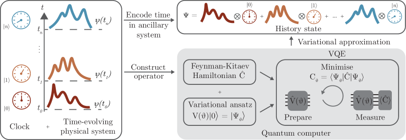
Figure 1: Sketch of the VFK method. Coupling the physical system to an auxiliary clock system we can encode an entire time evolution into a time-independent state. We prepare a variational approximation of the history state by measuring the expectation value of Feynman-Kitaev Hamiltonian and its derivatives on quantum computer.

II.2 Efficient mapping on Quantum hardware

We want to encode the history state on the qubits of a quantum computer, therefore we need to find an efficient mapping for the Feynman-Kitaev Hamiltonian onto qubit operators. The physical and auxiliary subsystems are encoded into a different partition of qubits. For the physical system, we will resort to one of the many established mappings [50, 51]. The auxiliary register, instead, is a $n+1$-level system and there are in principle combinatorially many ways to map it to qubits [52]. In this work we considered both the standard binary and the Gray mapping [53] to encode every state $\ket{i}$ into a bit string state. Since $n_{a}$ binary digits have $2^{n_{a}}$ different values, encoding $n$ different time steps requires $n_{a}=\log_{2}(n)$ auxiliary qubits using those mappings. The main difference among binary and Gray encoding is how many (qu-)bits must be flipped when going from one time-step $\ket{i}$ to the next. Under binary encoding one will eventually need to flip all qubits, such as when going from $\ket{i=3}\leftrightarrow\ket{011}$ to $\ket{i=4}\leftrightarrow\ket{100}$ in the case of $n_{a}=3$. Gray code, instead, is built in order to flip only one bit at every step, and therefore the time-step operator $\outerproduct{i}{i+1}$ can be implemented with a single qubit rotation on 1 qubit.

Consider the time step $\ket{i}$ and its Gray binary mapping $\ket{x_{n_{a}}\dots x_{2}x_{1}}$, $x_{i}\in\{0,1\}\,\,\forall i$. Let $x_{j}$ be the difference bit between $|i\rangle$ and $|i+1\rangle$. Then, the auxiliary forward operator has the form

$$\outerproduct{i+1}{i}=\outerproduct{x_{n_{a}}}{x_{n_{a}}}\otimes\dots\otimes\outerproduct{\neg x_{j}}{x_{j}}\otimes\dots\otimes\outerproduct{x_{1}}{x_{1}}$$ (6)

where $\neg$ indicates the negation of the bit value. This is a tensor product of operators acting on single qubits. Then, each term is mapped onto qubit operators using the following equalities:

$$\outerproduct{x}{x} =\frac{1}{2}\big{(}\hat{\mathbf{I}}+(-1)^{x}\hat{\sigma}^{z}\big{)}\,,$$ (7)

$$\outerproduct{\neg x}{x} =\frac{1}{2}\big{(}\hat{\sigma}^{x}+(-1)^{x}i\hat{\sigma}^{y}\big{)}\,,$$

where $\hat{\sigma}^{x}$, $\hat{\sigma}^{y}$ and $\hat{\sigma}^{z}$ indicate the Pauli operators. The same considerations apply to the backward auxiliary operator and the projectors.

The last term to consider is the time evolution operator $U(dt)$. In general, it is not possible to prepare $\hat{U}(dt)$ exactly in an efficient way if the Hamiltonian contains non-commuting terms. For this reason we will consider the Trotter-Suzuki approximation of the time evolution operator [54, 55].

Having shown how to prepare the Feynamn-Kitaev as a qubit operator, we can now use the Variational Quantum Eigensolver (VQE) [23] with such Hamiltonian to optimise the variational parameters of a quantum circuit in order to obtain an approximation of the history state. Considering a unitary variational circuit ansatz $\ket{\Psi_{\theta}}=\hat{V}(\theta)\ket{0}$, we will use the quantum computer to measure $E_{\theta}=\bra{\Psi_{\theta}}\hat{C}\ket{\Psi_{\theta}}$ and its derivatives. Iteratively, a classical processor will determine new values of $\theta$ to minimize $E_{\theta}$. We remark that minimising $E_{\theta}$ has been proved to be equivalent to the application of McLachlan’s variational principle [48, 42]. In the following, we will refer to the whole procedure as Variational Feynman Kitaev (VFK) method.

Once a variational approximation of the history state is obtained, we measure expectation values of observables $\hat{O}$ on the system at time step $t$ using the following equality:

$$\expectationvalue{\hat{O}(t)}=\bra{\psi_{t}}\hat{O}\ket{\psi_{t}}\sim\bra{\Psi_{\theta}}\big{[}\hat{O}\otimes\outerproduct{t}{t}\big{]}\ket{\Psi_{\theta}}\,.$$ (8)

An sketch of the method is shown in Fig. 1, while example applications of the final variational history state can be found in Section III.

II.3 Computational cost on quantum hardware of the Feynman-Kitaev Hamiltonian

In this Section we analyze the computational cost of measuring the Feynman-Kitaev Hamiltonian in Eq. 4 on a quantum device. First, we estimate the number of Pauli strings acting on the clock $n_{\textrm{Pauli}}^{c}$ and on the physical system $n_{\textrm{Pauli}}^{p}$. Then, the total number of Pauli strings will be $n_{\textrm{Pauli}}^{\textrm{tot}}\leq n_{\textrm{Pauli}}^{p}*n_{\textrm{Pauli}}^{c}$ .

Given a number of time steps $n$, or $n_{a}=\log_{2}n$ auxiliary qubits to encode them, we can determine how many Pauli strings will make up the operators acting on the auxiliary system. The terms in $C_{0}$ and $C_{1}$ are projectors $\outerproduct{i}{i}$ with $i\in\{0,\dots,n\}$, can be expressed as $2^{n_{a}}$ combinations of $\hat{\mathbf{I}}$ and $\hat{\sigma}^{z}$ as indicated in Eq. 7 that can be measured all at once. On the contrary, $C_{2}$ contains the forward and backward unitaries, resulting in $n\log_{2}n=n_{a}2^{n_{a}}$ different Pauli strings.

For the physical system, we approximated the time evolution operator with a single Trotter-Suzuki step of size $dt$. The unitary operation corresponding to a Trotter step is not local if the terms of the physical Hamiltonian do not commute, giving a final number of different Pauli strings exponential in the physical qubits, a behaviour that may hinder scalability of the proposed method. For this reason, we have to resort to a different strategy. Consider the $m$ sets of non-commuting operators $H_{m}$ that constitute the physical Hamiltonian $H=\sum_{m}H_{m}$. We can rewrite the operator $C_{2}$ as

$$\hat{C}_{2}=\sum_{i=0}^{n^{\prime}-1}\sum_{j=0}^{m-1}\hat{U}_{j}(dt)\otimes\outerproduct{ij+1}{ij}+\hat{U}_{j}^{\dagger}(dt)\otimes\outerproduct{ij}{ij+1}$$ (9)

where $U_{j}(dt)=e^{-iH_{j}dt}$ is the $j$-th set of commuting operators, that can be exactly Trotterized, and $n^{\prime}=\lfloor\frac{n}{m}\rfloor$. The physical part of the Feynman-Kitaev Hamiltonian will have $m$ sets of commuting Pauli strings, since all the strings inside the same set can be measured at once. This strategy reduces the number of Trotter steps we can encode into $n_{a}$ auxiliary qubits from $n$ to $n^{\prime}$, but reduces the computational cost from exponential to polynomial in the number of physical spins. In Section III we show how to implement this strategy for the physical system under consideration.

II.4 Dynamical quantum phase transitions

Given a quantum system governed by the Hamiltonian $\hat{H}$ with initial state $|\psi(0)\rangle$, the Loschmidt echo is defined by

$$L(t)\equiv\absolutevalue{\bra{\psi(0)}e^{-i\hat{H}t}\ket{\psi(0)}}^{2}=\absolutevalue{\innerproduct{\psi(0)}{\psi(t)}}^{2}\,.$$ (10)

Loschmidt echoes are important quantities in many-body theory and appear in various contexts such as quantum chaos [56, 57] or the Schwinger’s particle production mechanism [58, 59]. In particular, we will consider the measurement of Loschmidt echoes for the identification of dynamical quantum phase transitions (DQPT) [60, 49]. Because the variational history state encodes the superposition of all different time-evolved physical states $\ket{\psi(t)}$ we will show in the following that it is computationally cheap to evaluate the Locshmidt echo on it.

Dynamical phase transitions can be identified by a nonanalytic behavior of the Lochsmidt echo and of its rate function $\lambda(t)$

$$\lambda(t)=-\lim_{D\rightarrow\infty}\frac{1}{D}\log\left[L(t)\right]$$ (11)

where $D$ is the number of degrees of freedom in our quantum system. Such phase transitions have been identified in many quantum systems [49] and also observed in experiments performed on analog quantum simulators [61, 62, 63].

In the following, we will show how to use the VFK method to study these phenomena. Assuming that the variational parameters of a circuit approximating the history state are obtained, we use an additional qubit to perform an Hadamard test [64] and measure the real and the imaginary part of $\innerproduct{\psi(t_{i})}{\psi(t_{j})}$ in order to calculate the Loschmidt echo. This only requires an additional qubit and the gate overhead required to calculate the Loschmidt echo with VFK state is negligible with respect to the total number of gates of the variational state.

A more detailed explanation of the Hadamard test, as well as the complete circuit, can be found in Appendix D, while an application of this method is reported in Section III.

III Results

To demonstrate the viability of the VFK method, we consider the Transverse Field Ising Model on an open 1-dimensional chain,

$$\hat{H}=J\sum_{i=0}^{n_{s}-1}\hat{\sigma}^{z}_{i}\hat{\sigma}^{z}_{i+1}+h\sum_{i=0}^{n_{s}}\hat{\sigma}^{x}_{i}\quad.$$ (12)

The first term accounts for interaction between spins while the latter represents a local and uniform magnetic field along the transverse direction $x$. For our simulations, we considered $J=\frac{1}{4}$, $h=1$. We use a classical computer to simulate the quantum hardware in an ideal case, without noise sources and with full access to the state vector produced by the quantum circuit (state-vector simulations). The simulations have been performed both in Python using IBM’s open-source library for quantum computing, Qiskit [65], and in Julia [66] with the Yao.jl [67] and PastaQ [68] frameworks. The code can be found at [69, 70].

We considered a variational ansatz of the form

$$\hat{V}(\theta)=\prod_{l=1}^{d}\Bigg{[}\prod_{\begin{subarray}{c}a\in A\end{subarray}}\bigg{(}\prod_{\begin{subarray}{c}i\neq j\\ i,j\in P\end{subarray}}\hat{G}_{ij,l}\prod_{\begin{subarray}{c}p\in P\end{subarray}}\hat{G}_{ap,l}\bigg{)}\Bigg{]}$$ (13)

where we denoted the set of qubits encoding the physical system $P$ and the set of auxiliary qubits $A$, while $G_{ij,l}$ is a parameterised gate of the form

@C=1em @R=1.5em & 1^G
G     =     @C=1em @R=1em & ^R_x(θ_1) ^R_y(θ_2) 1
^R_x(θ_3) ^R_y(θ_4)

The total number of blocks, or depth, is $d$. The total number of variational parameters is then given by

$$n_{pars}=2dn_{a}(n_{s}^{2}+n_{s})$$ (14)

where $n_{s}$ and $n_{a}$ indicate the number of spin and auxiliary qubits, respectively.

The Ising Hamiltonian in Eq. 12 has two sets of non commuting operators $H_{X}=\sum_{i=0}^{n_{s}}\hat{\sigma}^{x}_{i}$ and $H_{ZZ}=\sum_{i=0}^{n_{s}-1}\hat{\sigma}^{z}_{i}\hat{\sigma}^{z}_{i+1}$. We make use of the strategy presented in Section II.3 in order to have a polynomial cost. We build the Feynman-Kitaev Hamiltonian by applying $U_{X}(dt)=\exp[-iH_{X}dt]$ at even clock values and $U_{ZZ}(dt)=\exp[-iH_{ZZ}dt]$ at the odd ones. The new amount of Trotter step that can be encoded in $n_{a}$ auxiliary qubits will be $n^{\prime}=\frac{n}{2}$.

First, we considered a system with $n_{s}=6$ spins and up to $n_{a}=6$ auxiliary qubits for a total simulation time $T_{e}=3$. We used the variational wavefunctions obtained with VFK to estimate expectation values of physical quantities as indicated in Eq. 8. In particular, we evaluated the total magnetization along the $z$ axis

$$\sigma^{z}=\frac{1}{n_{s}}\sum_{i=1}^{n_{s}}\sigma^{z}_{i}$$ (15)

through the entire time evolution. To assess the accuracy of these variational history states obtained with the VFK method, we measured the infidelity $1-F_{\text{VFK}}$ with respect to Trotter-Suzuki wavefunctions. For every simulated time $t_{i}$, we prepared the Trotter-Suzuki state $|\psi_{i}^{TS}\rangle=\hat{U}^{i}_{TS}(dt)|\psi(0)\rangle$ with $dt=\frac{T_{e}}{2^{n_{a}-1}}$ and evaluated the infidelity with VFK history state projected onto the $|i\rangle$ subspace. Results are reported in Fig. 2.

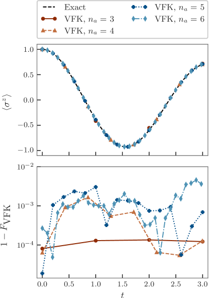
Figure 2: Magnetization (top) and infidelities (bottom) measured on the VFK history state. We considered a system of $n_{s}=6$ spins initialised in $|0\rangle^{\otimes 6}$ and different auxiliary qubits $n_{a}$ for a simulation time $T_{e}=3.0$. $F_{\text{VFK}}$ at time $t_{i}$ indicates the fidelity measured between the Trotter-Suzuki state with $i$ steps and the VFK state projected on the $|i\rangle$ subspace.

Increasing the number of auxiliary qubits while keeping the total simulation time $T_{e}$ fixed decreases the size of a single Trotter step, decreasing also the error with respect to the exact state. We remark that, if the variational ansatz is able to reproduce exactly the history state, the variational history state can be as accurate as the corresponding Trotter-Suzuki approximation.

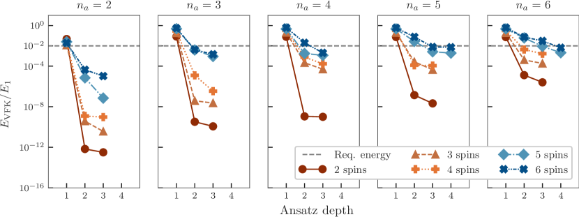
Figure 3: Final energy obtained with the VFK algorithm ($E_{\text{VFK}}$) over the energy of the first excited state ($E_{1}$) obtained using a classical simulator. The plot shows the final energy obtained for a system of $n_{s}$ spins and $2^{n_{a}-1}$ time steps as a function of the depth of ansatz in Eq. 13. The gray, dashed lines indicate the energies we require to consider the VFK converged. We fixed the simulation time $T_{e}=3.0$, therefore increasing the number of auxiliary qubits reduces the time step and the Trotter-Suzuki approximation error, accordingly. The corresponding fidelities can be found in Appendix C

We run multiple simulations for varying system and clock sizes $n_{s},n_{a}\in\left[2,3,4,5,6\right]$. The ground-state optimisation is performed using the Variational Quantum Eigensolver (VQE) algorithm and the ADAM optimiser [71]. The time evolution unitaries in the target Feynman-Kitaev Hamiltonian are smoothly varied from $\hat{U}(dt=0)$ to $\hat{U}(dt=T_{e}/2^{n_{a}-1})$ in order to help the convergence of the method (see Appendix B for additional details).

During the optimisation we monitor the energy of the state, which we showed to bound the infidelity with respect to the target state. Once it gets below a certain threshold, we stop the optimisation and consider that we have reached convergence. Since the energy of the first excited states of the Feynman-Kitaev Hamiltonian decreases as the number of auxiliary qubits increases, the threshold is chosen to be $10^{-2}\cdot E_{1}$, where $E_{1}$ indicates the energy of the first excited state. As indicated in [38], $E_{1}$ can be derived analytically from an unitarily equivalent Hamiltonian and its value is $E_{1}=1-\cos(\pi/2^{n_{a}})$. For this reason, we are able to use $E_{1}$ as convergence threshold.

The complexity of the optimisation procedure increases with the number of auxiliary qubits, however we are able to reach convergence by increasing the ansatz depth $d$. This is consistent with the fact that preparing the exact history state would require an exponentially deep circuit with the clock system size. In Fig. 3 we report the final energies obtained as a function of the ansatz depth. For comparison, in Appendix C we report the infidelities with respect to the exact ground state for the same calculations.

Then, we considered the smallest depth necessary to reach convergence, and compared the number of two-qubit gates needed by the variational-circuit with the number of two-qubit gates needed by a standard Trotter-Suzuki circuit with the same number of time-steps. The results are indicated in Fig. 4. We only report the comparison for two qubit gates and not for one-qubit gates because the latters are usually not a bottleneck in NISQ devices.

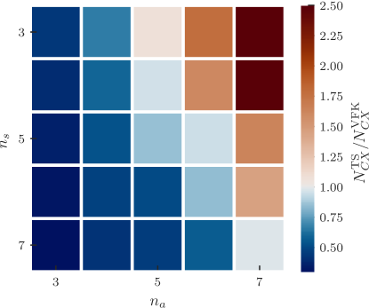
Figure 4: Comparison between two-qubits gates required by the Trotter-Suzuki circuit ($N^{TS}_{\text{CX}}$) and by the variational ansatz ($N^{\text{VFK}}_{\text{CX}}$), given the same system size and Trotter steps. $N^{\text{VFK}}_{\text{CX}}$ corresponds to the minimal circuit required to make VFK converge and depends on ansatz type and depth. $N^{TS}_{\text{CX}}$ is fixed, given system size and number of steps. We considered the ansatz in Eq. 13 and a simulation time $T_{e}=3.0$.

In Fig. 4 we show that the VFK history state has an overhead compared to Trotter if few time-steps are considered, but as the number of time-steps is increased, VFK method has a favorable scaling. Moreover, the VFK history state contains more information than the state obtained at the end of the Trotter evolution, which can be used, for example, to compute Lochsmidt echoes.

In this regard, we show that the VFK variational wavefunction can be used to study dynamical quantum phase transitions. We still consider the Transverse-Field Ising Model with $J=1/4$ and $h=1$. As the equilibrium model exhibits a quantum phase-transition in the ground-state when going from $h<J$ to $h>J$, a dynamical quantum phase transition is known to appear if the system is quenched from one region to the other [49].

We consider a system initialised at $|\psi(0)\rangle=|0\rangle^{\otimes n_{s}}$, the ground-state of the Hamiltonian for $h=0$, and we then compute the VFK history state using the same procedure described before for $T_{e}=3$, $h=1$ and varying system sizes. After determining the optimal parameters, we used the Hadamard test to evaluate the rate function of the Loschmidt echo as described in Appendix D. In Fig. 5 we show that a nonanalytic behaviour appears as the system size grows. We are able to improve the time-resolution by increasing the number of auxiliary qubits. As the number of spins approaches the thermodynamic limit, the qubit overhead required to characterise the cusp becomes negligible.

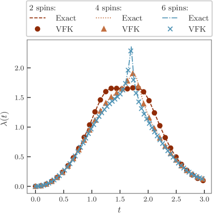
Figure 5: Rate function of the Loschmidt echo in the Transverse Field Ising Model measured using the VFK variational state. The plot shows a dynamical phase transition for an open chain initialised in the $|0\rangle^{\otimes n_{s}}$ state and evolved under the Hamiltonian in Eq. 12. The nonanalyticity appears when the number of spin is increased. We considered a number of auxiliary qubits $n_{a}=6$ for $n_{s}=2,4$ and $n_{a}=7$ for $n_{s}=6$.

Finally, we investigate the algorithm performance in the presence of noise. We follow the noise model proposed by Kandala, Mezzacapo et al. in [47], where the effects of decoherence are approximated by an amplitude damping and dephasing channel acting after each fundamental gate on the system density matrix $\rho$ as

$$\rho \rightarrow E^{a}_{0}\rho E^{a\dagger}_{0}+E^{a}_{1}\rho E^{a\dagger}_{1}\,,$$ (16)

$$\rho \rightarrow E^{d}_{0}\rho E^{d\dagger}_{0}+E^{d}_{1}\rho E^{d\dagger}_{1}$$

with

$$E^{a}_{0}=\begin{bmatrix}1&0\\ 0&\sqrt{1-p^{a}}\\ \end{bmatrix}\,,\,E^{a}_{1}=\begin{bmatrix}0&\sqrt{p^{a}}\\ 0&0\\ \end{bmatrix}$$ (17)

and

$$E^{d}_{0}=\begin{bmatrix}1&0\\ 0&\sqrt{1-p^{d}}\\ \end{bmatrix}\,,\,E^{d}_{1}=\begin{bmatrix}0&0\\ 0&\sqrt{p^{d}}\\ \end{bmatrix}\,.$$ (18)

The fundamental gates are taken to be CNOT, $\hat{R}_{x}$, $\hat{R}_{y}$ and $\hat{R}_{z}$; all other gates, such as the $\hat{R}_{zz}$ used in the Trotter circuit, are decomposed into a sequence of those gates. The 1- and 2- qubit error rates $p^{a,d}_{1}$ and $p^{a,d}_{2}$ are estimated from QPU data such as the relaxation and dephasing time available at [1, 4]. More details on the estimation of the error rates can be found in Appendix E.

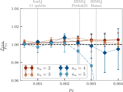
Figure 6: Comparison between the mean infidelity of noisy VFK and Trotter-Suzuki circuits through a time evolution to $T_{e}=3.0$. Markers indicate the mean value, while the bars the standard deviation over a time evolution. We fixed the error probability for single qubit gates $p_{1}=2\cdot 10^{-4}$. We considered a system with $n_{s}=2$ and different number of auxiliary qubits $n_{a}$, Trotter steps are varied accordingly. The horizontal line indicates equal mean fidelity between VFK and Trotter-Suzuki circuits. Vertical lines indicate the mean $p_{2}$ error probability for reference devices.

In Fig. 6 we compare the mean fidelity $F_{\text{VFK}}$ obtained from the VFK calculation on noisy system of $n_{s}=2$ spins and different $n_{a}$ against the mean fidelity of the trotter evolution $F_{\text{TS}}$ (we take the fidelity to be $F(\rho,\sigma)=\left[\textrm{Tr}\left(\sqrt{\sqrt{\rho}\sigma\sqrt{\rho}}\right)\right]^{2}$, where $\rho,\sigma$ are two density matrices). We study how their ratio $F_{\text{VFK}}/F_{\text{TS}}$ varies as a function of different 2-qubit error rates $p^{a}_{2}=p^{d}_{2}=p_{2}$, while keeping the single qubit error rate constant to an average value $p^{a}_{1}=p^{d}_{1}=p_{1}=2\cdot 10^{-4}$ that is consistent with real-world devices. This approach is motivated by the fact that today’s devices are mainly limited in the fidelity they can achieve when performing 2-qubit operations.

The plot indicates comparable performances between the two methods, with an advantage of VFK for $n_{a}=2,3$. As the number of auxiliary qubits is increased to $n_{a}=4,5$, the VFK optimisation must converge towards smaller values of the energy in order to give sensible results. However, at higher error rates we were not able to succesfully optimise the variational parameters, which can be seen in the figure by the fact that the performance of the VFK method then degrades. To give a better idea of where today’s QPUs stand, some vertical lines represent the mean values of $p_{2}$ for commercially-available devices, which shows that Ion-based setups have a low-enough error rate and could be able to use the VFK algorithm efficiently already today.

IV Conclusions and outlook

In this work we showed a strategy to study dynamical properties of a quantum system using variational ground-state quantum algorithms. Our method, which we called variational-Feynman Kitaev (VFK), combines the Feynman-Kitaev Hamiltonian together with existing variational-ground state methods in order to study dynamical systems with the limited resources available on today’s NISQ devices.

First, we showed how the Feynman-Kitaev Hamiltonian can be efficiently implemented on a quantum computer using a binary encoding for the auxiliary system and the Trotter-Suzuki approximation for the time evolution operator. Then, we demonstrated our method studying the transverse field Ising model and showing that it scales favorably compared to a Trotter-Suzuki evolution when many time-steps are needed. We investigated the convergence of the algorithm as the number of spins and auxiliary qubits increases and compared the final circuits with the corresponding Trotter-Suzuki approximation. Considering a noise model accounting for decoherence, we assessed that our algorithm yields slightly better results than a plain Trotter evolution when the two qubits error rate is not too detrimental. As analysed in [46], variational methods are robust against certain types of quantum errors, a promising feature for future hardware demonstrations. Finally, we showed that it is possible to exploit the structure of the VFK history state to measure dynamical quantities such as the Loschmidt echo efficiently, and gave an example of how to detect dynamical quantum phase transitions in the Transverse Field Ising model.

As a future research direction, we believe that it would be of interest to investigate the application of the VFK method to other physical systems, as well as its application to estimate quantities that are not easily accessible via standard Trotterisation. Similarly to all other variational algorithms, the choice of the right ansatz is fundamental for the algorithm to succeed. In the ansatz we proposed, the gates required between auxiliary and system qubits currently limit the implementation on hardware. However, we envision application of the method in devices with high qubit connectivity. Moreover, we showed that once the variational history state is obtained, it has applications beyond the evaluation of expectation values of time-dependent observables.

Data availability

The code used to run the simulations is open source and can be found at [69, 70].

Appendix A Comparison with projected - Variational Quantum Dynamics

In this Appendix we compare the VFK method to the p-VQD method presented in [29]. We consider the same TFIM in Eq. 12 and the same parameters. The p-VQD variational state is prepared using the ansatz presented in [29]. We define the mean integrated infidelity

$$\delta_{F}(T_{e})=\frac{1}{T_{e}}\int_{t=0}^{T_{e}}\left(1-|\innerproduct{\psi_{TS}(t)}{\psi_{\theta_{t}}}|^{2}\right)dt=\frac{\Delta_{F}(T_{e})}{T_{e}}$$ (19)

where $|\psi_{TS}(t)\rangle$ is the Trotter-Suzuki state prepared at time $t$, while $|\psi_{\theta_{t}}\rangle$ indicates the variational state that approximates it. In the VFK method, the variational history state $|\Psi_{\theta}\rangle$ is prepared and projected onto the $|t\rangle$ subspace before calculating the fidelity. We fix a total simulation time $T_{e}$ and the number of auxiliary qubits in the VFK method determine the number of time steps for both methods. Given that, differently from VFK, the variational wavefunction prepared by the p-VQD algorithm encodes the evolution of the quantum state only at certain time $t$, the ansätze used in the two methods are different. For VFK, the ansatz is the same presented in Eq. 13, with depth of converged calculations in Fig. 3. For p-VQD, we use the same ansatz presented in [29] with depth $d=3$, resulting in a total number of $d*(n_{s}+(n_{s}-1))+n_{s}=7n_{s}-3$ free parameters.

We use the ADAM optimiser and a comparable number of optimisation steps. Results of this comparison are shown in Fig. 7.

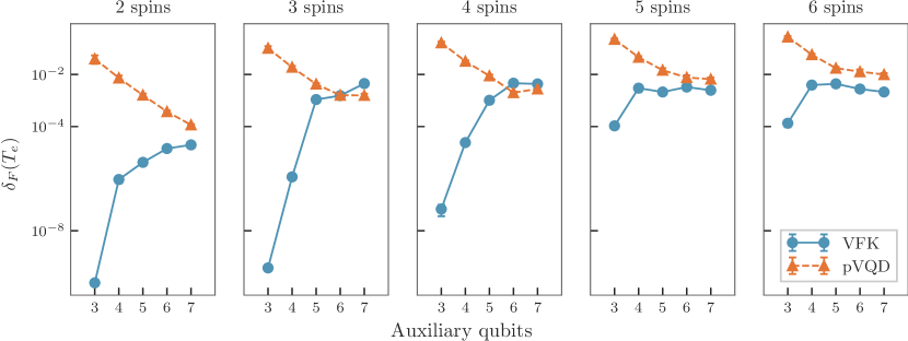
Figure 7: Mean infidelity over an entire time evolution as a function of the number of spins and auxiliary qubits. The plot compares the mean infidelity between the variational state obtained with VFK (after projecting to $|t\rangle$ subspace) or p-VQD and the exact state. For the VQE we used the ansatz in Eq. 13, while for p-VQD the alternating rotations ansatz presented in [29]. We considered a total simulation time $T_{e}=3.0$ and a number of optimisation steps comparable between the two methods. The analysis is performed using a state-vector simulator and the ADAM optimiser for both methods.

When the number of time steps is small, the infidelity of the VFK method is lower. If we choose a time step small enough we are able to improve the accuracy of the p-VQD method, thanks to parameter optimisation at every time step. Provided a converged optimization, they are expected to converge to the same mean integrated infidelity in the limit of infinite time steps.

Appendix B Optimisation strategy

As a variational algorithm, the optimisation of the wavefunction using VQE can be hindered by local minima or the presence of barren plateaus [72, 73, 74]. In particular, the definition of the cost function in terms of global observables leads to the emergence of such plateaus even when $V(\theta)$ is a shallow circuit [74]. To improve the optimisation procedure, we devise a specific strategy. Consider $dt=0$, in this case the history state has the form

$$\ket{\Psi_{0}}=\frac{1}{\sqrt{n+1}}\sum_{i=0}^{n}\ket{\psi(0)}\ket{i}\,.$$ (20)

When $dt$ is infinitesimal, the history state $\ket{\Psi}$ is infinitesimally close to $\ket{\Psi_{0}}$. Assuming $\ket{\psi(0)}$ is a simple state to prepare or, equivalently, that we have an efficient approximation to it, we start with the circuit in the state $\ket{\Psi_{0}}$ and initialize the variational gates as identity operators. Then, we substitute every $\hat{U}(dt)$ in the Feynman-Kitaev Hamiltonian with its $k$-root $\sqrt[k]{\hat{U}(dt)}=\hat{U}(dt/k)$. Considering $k$ large enough, we can start the optimisation close to the optimum. Finally, we optimise the wavefunction for decreasing $k$ until $k=1$ and the targeted clock Hamiltonian is obtained. In general, every function $f(dt,k)$ can be considered and the Feynman-Kitaev Hamiltonian built upon $\hat{U}[f(dt,k)]$, e.g. $f(dt,k)=dt\frac{k}{k_{0}}$ with $k\in\{1,\dots,k_{0}\}$ and $k_{0}$ an arbitrary large number.

Appendix C Fidelity of the VQE calculations

In this Appendix we show the fidelity between the variational state obtained with the VFK algorithm and the corresponding exact history state. As explained in Section II.1, the fidelity is upper bounded by the normalized energy. Indeed, given a state $\ket{\phi}=\sqrt{1-\epsilon^{2}}\ket{\Psi}+\epsilon\ket{\delta}$ close to the target state $\ket{\Psi}$, where $\epsilon\approx 0,\,\,\innerproduct{\Psi}{\delta}=0$, we can calculate its fidelity and energy as a function of $\epsilon$.

In particular, we obtain that $1-F(\phi,\Psi)=\epsilon^{2}$ and $E(\ket{\phi})=\epsilon^{2}E(\ket{\delta})$, where we defined $F(\phi,\Psi)=|\langle\phi|\Psi\rangle|^{2}$ and to calculate $E(\ket{\phi})$ we considered that $E(\ket{\Psi})=0$ by construction. Given that $\ket{\delta}$ is orthogonal to $\ket{\Psi}$, $E(\ket{\delta})\geq E_{1}$, where $E_{1}$ is the energy of the first excited state. For this reason, we can conclude that the infidelity is upper bounded by the energy normalized by $E_{1}$, which can be calculated analytically, as shown in [38]. In Fig. 8 we report the infidelities for states whose energy is shown in Fig. 3

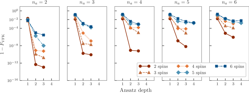
Figure 8: Final infidelities of the states obtained with the VFK algorithm ($1-F_{\text{VFK}}$) using a classical simulator with respect to the exact history state. The plot report the infidelities corresponding to the calculations presented in Fig. 3.

Appendix D Measuring Loschmidt echoes

In this Appendix, we illustrate how to extend the VFK circuit in order to measure Loschmidt echoes. Consider the overlap between the system quantum state evolved at two different times $t_{i}$ and $t_{j}$, namely $\innerproduct{\psi(t_{i})}{\psi(t_{j})}$. In general, this quantity is complex, therefore we have to perform an Hadamard test to evaluate its real and imaginary part. In the following, we describe how to measure the real part; the same procedure applies for the imaginary part, with a slight modification.

First, we define the time-swap operator as

$$\hat{\text{T}}_{\text{SWAP}}(t_{i},t_{j})=\bigotimes_{k\in T_{ij}}\hat{\sigma}^{x}_{k}\,,$$ (21)

where $T_{ij}$ indicates the set of bits that differs in the bit string encoding of $t_{i}$ and $t_{j}$. We use the set of parameters obtained with the VFK method to initialise the variational circuit $V(\theta)$. We control the action of the time-swap operator over the clock system using an additional auxiliary qubit initialized in $|+\rangle=\frac{|0\rangle+|1\rangle}{\sqrt{2}}=H|0\rangle$. In the following, we will refer to the qubits of the auxiliary clock system as the clock qubits, to distinguish them from the auxiliary qubit added to perform the Hadamard test. Then, we apply again an Hadamard gate to the auxiliary qubit and we measure the auxiliary and the clock qubits. We post-select the measurements in which the measurement of the clock system returns the binary string corresponding to $t_{i}$ (or $t_{j}$). We indicate the number of post-selected measurements with the auxiliary qubit in $0$ ($1$) as $N_{0}$ ($N_{1}$).

Finally , the real part of the overlap will be

$$\innerproduct{\psi(t_{i})}{\psi(t_{j})}=2^{n_{a}}\frac{N_{0}-N_{1}}{N_{\text{shots}}}$$ (22)

where $N_{\text{shots}}$ indicates the number of times the system has been prepared and measured, while the prefactor $2^{n_{a}}$ is required for the normalisation of the history state. Considered a system with $2$ system qubits and a single clock qubit, the final circuit to measure the real part of $\innerproduct{\psi(t_{0})}{\psi(t_{1})}$ has the form

@C=1em @R=1.5em |0⟩ & H 1 H
A 2V(θ)
V(θ)
V(θ) 34.8em.8emP

where $P$ indicates the two system qubits and $A$ the clock qubit. To measure the imaginary part of the overlap, the same procedure applies, with the auxiliary qubit initialised in $\frac{|0\rangle-i|1\rangle}{\sqrt{2}}=HS^{\dagger}|0\rangle$.

Appendix E Noise model for the numerical experiments

In this Appendix, we describe how we included decoherence effects in the numerical simulations shown in Fig. 6. As indicated in the main text, we followed the noise model proposed by Kandala et al. in [47], where the effects of decoherence are approximated by the successive application of an amplitude damping and dephasing channel acting after each gate on the system density matrix

$$\rho \rightarrow E^{a}_{0}\rho E^{a\dagger}_{0}+E^{a}_{1}\rho E^{a\dagger}_{1}\,,$$ (23)

$$\rho \rightarrow E^{d}_{0}\rho E^{d\dagger}_{0}+E^{d}_{1}\rho E^{d\dagger}_{1}$$

with

$$E^{a}_{0}=\begin{bmatrix}1&0\\ 0&\sqrt{1-p^{a}}\\ \end{bmatrix}\,,\,E^{a}_{1}=\begin{bmatrix}0&\sqrt{p^{a}}\\ 0&0\\ \end{bmatrix}\,\,\,\,\,\,\text{and}\,\,\,\,\,\,E^{d}_{0}=\begin{bmatrix}1&0\\ 0&\sqrt{1-p^{d}}\\ \end{bmatrix}\,,\,E^{d}_{1}=\begin{bmatrix}0&0\\ 0&\sqrt{p^{d}}\\ \end{bmatrix}\,.$$ (24)

The error rates $p^{a}$ and $p^{d}$ can be determined from actual device data. In particular, we have

$$p^{a}=1-e^{-\tau/T_{1}}\,\,\,,\,\,\,p^{d}_{g}=1-e^{-2\tau/T_{\phi}}$$ (25)

where $T_{1}$ is the relaxation time of the qubit, $\tau$ is the gate time and $T_{\phi}=2T_{1}T_{2}/(2T_{1}-T_{2})$, given $T_{2}$ the coherence time of the qubit. When the time of a single- or two- qubit gate is substituted in $\tau$, we obtain $p^{a,d}_{1}$ and $p^{a,d}_{2}$, respectively. We used data found in [1, 4] to estimate an average value of $p^{a,d}_{1}$ and a range of $p^{a,d}_{2}$ to analyze in our simulations. Finally, in order to simplify the comparison in Fig. 6, we considered $p^{a}=p^{d}$ for both single- or two- qubit gates. This approximation holds when $T_{1}\sim T_{2}$, which is true on an average basis for superconducting devices [1].

For completeness, we report in Table 1 the data of the devices indicated in Fig. 6.

Device	$T_{1}$ $(\mu s)$	$T_{2}$ $(\mu s)$	$\tau_{2}$ $(\mu s)$	$\tau_{1}$ $(\mu s)$
IBMQ Peekskill	250.12	242.82	0.420571	0.0035
IBMQ Hanoi	160.64	144.7	0.318603	0.0035
IonQ 11 qubits	$>10^{7}$	$2*10^{5}$	210	10

Table 1: Average coherence values and gate times of the devices indicated in Fig. 6, as of March 2022.

References

- IBM [2022] IBM, IBM Quantum services (Accessed March 2022).
- Google [2022] Google, Google AI Quantum hardware (Accessed March 2022).
- Wright et al. [2019] K. Wright et al., Benchmarking an 11-qubit quantum computer, Nature Communications 10, 5464 (2019).
- IonQ [2022] IonQ, IonQ devices and providers (Accessed March 2022).
- Shor [1994] P. Shor, Algorithms for quantum computation: discrete logarithms and factoring, in Proceedings 35th Annual Symposium on Foundations of Computer Science (IEEE Comput. Soc. Press, 1994).
- Grover [1996] L. K. Grover, A fast quantum mechanical algorithm for database search, in Proceedings of the Twenty-Eighth Annual ACM Symposium on Theory of Computing, STOC ’96 (Association for Computing Machinery, New York, NY, USA, 1996) p. 212–219.
- Santoro and Tosatti [2006] G. E. Santoro and E. Tosatti, Optimization using quantum mechanics: quantum annealing through adiabatic evolution, Journal of Physics A: Mathematical and General 39, R393 (2006).
- Kassal et al. [2008] I. Kassal, S. P. Jordan, P. J. Love, M. Mohseni, and A. Aspuru-Guzik, Polynomial-time quantum algorithm for the simulation of chemical dynamics, Proceedings of the National Academy of Sciences 105, 18681 (2008).
- Georgescu et al. [2014] I. M. Georgescu, S. Ashhab, and F. Nori, Quantum simulation, Rev. Mod. Phys. 86, 153 (2014).
- Feynman [1982] R. P. Feynman, Simulating physics with computers, Int. J. Theor. Phys. 21, 467 (1982).
- Lloyd [1996] S. Lloyd, Universal quantum simulators, Science 273, 1073 (1996).
- Abrams and Lloyd [1997] D. S. Abrams and S. Lloyd, Simulation of many-body fermi systems on a universal quantum computer, Phys. Rev. Lett. 79, 2586 (1997).
- Cade et al. [2020] C. Cade, L. Mineh, A. Montanaro, and S. Stanisic, Strategies for solving the Fermi-Hubbard model on near-term quantum computers, Phys. Rev. B 102, 235122 (2020).
- Google AI Quantum and collaborators [2020] Google AI Quantum and collaborators, Observation of separated dynamics of charge and spin in the Fermi-Hubbard model (2020), arXiv:2010.07965 [quant-ph] .
- Cao et al. [2019] Y. Cao, J. Romero, J. P. Olson, M. Degroote, P. D. Johnson, M. Kieferová, I. D. Kivlichan, T. Menke, B. Peropadre, N. P. D. Sawaya, S. Sim, L. Veis, and A. Aspuru-Guzik, Quantum chemistry in the age of quantum computing, Chemical Reviews 119, 10856 (2019).
- Bauer et al. [2020] B. Bauer, S. Bravyi, M. Motta, and G. K.-L. Chan, Quantum algorithms for quantum chemistry and quantum materials science, Chemical Reviews 120, 12685–12717 (2020).
- Sheng et al. [2021] N. Sheng, C. Vorwerk, M. Govoni, and G. Galli, Quantum embedding theories to simulate condensed systems on quantum computers (2021), arXiv:2105.04736 [quant-ph] .
- Bassman et al. [2021] L. Bassman, M. Urbanek, M. Metcalf, J. Carter, A. F. Kemper, and W. A. de Jong, Simulating quantum materials with digital quantum computers, Quantum Science and Technology 6, 043002 (2021).
- Childs et al. [2018] A. M. Childs, D. Maslov, Y. Nam, N. J. Ross, and Y. Su, Toward the first quantum simulation with quantum speedup, Proceedings of the National Academy of Sciences 115, 9456 (2018).
- Babbush et al. [2018] R. Babbush, C. Gidney, D. W. Berry, N. Wiebe, J. McClean, A. Paler, A. Fowler, and H. Neven, Encoding electronic spectra in quantum circuits with linear t complexity, Phys. Rev. X 8, 041015 (2018).
- Nam and Maslov [2019] Y. Nam and D. Maslov, Low-cost quantum circuits for classically intractable instances of the Hamiltonian dynamics simulation problem, npj Quantum Information 5, 10.1038/s41534-019-0152-0 (2019).
- Motta et al. [2021] M. Motta, E. Ye, J. R. McClean, Z. Li, A. J. Minnich, R. Babbush, and G. K.-L. Chan, Low rank representations for quantum simulation of electronic structure, npj Quantum Information 7, 83 (2021).
- Peruzzo et al. [2014] A. Peruzzo, J. McClean, P. Shadbolt, M.-H. Yung, X.-Q. Zhou, P. J. Love, A. Aspuru-Guzik, and J. L. O’Brien, A variational eigenvalue solver on a photonic quantum processor, Nature Communications 5, 10.1038/ncomms5213 (2014).
- Li and Benjamin [2017] Y. Li and S. C. Benjamin, Efficient variational quantum simulator incorporating active error minimization, Phys. Rev. X 7, 021050 (2017).
- Motta et al. [2019] M. Motta, C. Sun, A. T. K. Tan, M. J. O’Rourke, E. Ye, A. J. Minnich, F. G. S. L. Brandão, and G. K.-L. Chan, Determining eigenstates and thermal states on a quantum computer using quantum imaginary time evolution, Nature Physics 16, 205–210 (2019).
- Ollitrault et al. [2020] P. J. Ollitrault, A. Kandala, C.-F. Chen, P. K. Barkoutsos, A. Mezzacapo, M. Pistoia, S. Sheldon, S. Woerner, J. M. Gambetta, and I. Tavernelli, Quantum equation of motion for computing molecular excitation energies on a noisy quantum processor, Phys. Rev. Research 2, 043140 (2020).
- Yuan et al. [2019] X. Yuan, S. Endo, Q. Zhao, Y. Li, and S. C. Benjamin, Theory of variational quantum simulation, Quantum 3, 191 (2019).
- Cerezo et al. [2021a] M. Cerezo, A. Arrasmith, R. Babbush, S. C. Benjamin, S. Endo, K. Fujii, J. R. McClean, K. Mitarai, X. Yuan, L. Cincio, and P. J. Coles, Variational quantum algorithms, Nature Reviews Physics 3, 625 (2021a).
- Barison et al. [2021] S. Barison, F. Vicentini, and G. Carleo, An efficient quantum algorithm for the time evolution of parameterized circuits, Quantum 5, 512 (2021).
- Lin et al. [2021] S.-H. Lin, R. Dilip, A. G. Green, A. Smith, and F. Pollmann, Real- and imaginary-time evolution with compressed quantum circuits, PRX Quantum 2, 010342 (2021).
- Barratt et al. [2021] F. Barratt, J. Dborin, M. Bal, V. Stojevic, F. Pollmann, and A. G. Green, Parallel quantum simulation of large systems on small NISQ computers, npj Quantum Information 7, 79 (2021).
- Otten et al. [2019] M. Otten, C. L. Cortes, and S. K. Gray, Noise-resilient quantum dynamics using symmetry-preserving ansatzes (2019), arXiv:1910.06284 [quant-ph] .
- Cîrstoiu et al. [2020] C. Cîrstoiu, Z. Holmes, J. Iosue, L. Cincio, P. J. Coles, and A. Sornborger, Variational fast forwarding for quantum simulation beyond the coherence time, npj Quantum Information 6, 10.1038/s41534-020-00302-0 (2020).
- Commeau et al. [2020] B. Commeau, M. Cerezo, Z. Holmes, L. Cincio, P. J. Coles, and A. Sornborger, Variational Hamiltonian diagonalization for dynamical quantum simulation (2020).
- Bharti and Haug [2021] K. Bharti and T. Haug, Quantum-assisted simulator, Physical Review A 104, 10.1103/physreva.104.042418 (2021).
- Benedetti et al. [2021] M. Benedetti, M. Fiorentini, and M. Lubasch, Hardware-efficient variational quantum algorithms for time evolution, Physical Review Research 3, 10.1103/physrevresearch.3.033083 (2021).
- Feynman [1985] R. P. Feynman, Quantum mechanical computers, Optics News 11, 11 (1985).
- Kitaev et al. [2002] A. Y. Kitaev, A. H. Shen, and M. N. Vyalyi, Classical and Quantum Computation (American Mathematical Society, USA, 2002).
- Caha et al. [2018] L. Caha, Z. Landau, and D. Nagaj, Clocks in Feynman's computer and Kitaev's local Hamiltonian: Bias, gaps, idling, and pulse tuning, Physical Review A 97, 10.1103/physreva.97.062306 (2018).
- Bausch and Crosson [2018] J. Bausch and E. Crosson, Analysis and limitations of modified circuit-to-Hamiltonian constructions, Quantum 2, 94 (2018).
- Giovannetti et al. [2015] V. Giovannetti, S. Lloyd, and L. Maccone, Quantum time, Physical Review D 92, 10.1103/physrevd.92.045033 (2015).
- McClean et al. [2013] J. R. McClean, J. A. Parkhill, and A. Aspuru-Guzik, Feynman’s clock, a new variational principle, and parallel-in-time quantum dynamics, Proceedings of the National Academy of Sciences 110, E3901–E3909 (2013).
- Tempel and Aspuru-Guzik [2014] D. G. Tempel and A. Aspuru-Guzik, The Kitaev–Feynman clock for open quantum systems, New Journal of Physics 16, 113066 (2014).
- McClean and Aspuru-Guzik [2015] J. R. McClean and A. Aspuru-Guzik, Clock quantum Monte Carlo technique: An imaginary-time method for real-time quantum dynamics, Phys. Rev. A 91, 012311 (2015).
- Watkins et al. [2022] J. Watkins, N. Wiebe, A. Roggero, and D. Lee, Time-dependent Hamiltonian simulation using discrete clock constructions (2022).
- McClean et al. [2016] J. R. McClean, J. Romero, R. Babbush, and A. Aspuru-Guzik, The theory of variational hybrid quantum-classical algorithms, New Journal of Physics 18, 023023 (2016).
- Kandala et al. [2017] A. Kandala, A. Mezzacapo, K. Temme, M. Takita, M. Brink, J. M. Chow, and J. M. Gambetta, Hardware-efficient variational quantum eigensolver for small molecules and quantum magnets, Nature 549, 242 (2017).
- McLachlan [1964] A. McLachlan, A variational solution of the time-dependent Schrodinger equation, Molecular Physics 8, 39 (1964).
- Heyl [2018] M. Heyl, Dynamical quantum phase transitions: a review, Reports on Progress in Physics 81, 054001 (2018).
- E.P. Jornan [1993] E. W. E.P. Jornan, The Collected Works of Eugene Paul Wigner (Springer, Berlin, Heidelberg, 1993).
- Bravyi and Kitaev [2002] S. B. Bravyi and A. Y. Kitaev, Fermionic quantum computation, Annals of Physics 298, 210 (2002).
- Sawaya et al. [2020] N. P. D. Sawaya, T. Menke, T. H. Kyaw, S. Johri, A. Aspuru-Guzik, and G. G. Guerreschi, Resource-efficient digital quantum simulation of d-level systems for photonic, vibrational, and spin-s Hamiltonians, npj Quantum Information 6, 49 (2020).
- Gray [1953] F. Gray, Pulse code communication (U.S. Patent 2 632 058, Mar. 1953).
- Trotter [1959] H. F. Trotter, Proc. Amer. Math. Soc. 10, 545 (1959).
- Suzuki [1991] M. Suzuki, General theory of fractal path integrals with applications to many-body theories and statistical physics, Journal of Mathematical Physics 32, 400 (1991).
- Peres [1984] A. Peres, Stability of quantum motion in chaotic and regular systems, Phys. Rev. A 30, 1610 (1984).
- Gorin et al. [2006] T. Gorin, T. Prosen, T. H. Seligman, and M. Žnidarič, Dynamics of Loschmidt echoes and fidelity decay, Physics Reports 435, 33–156 (2006).
- Schwinger [1951] J. Schwinger, On gauge invariance and vacuum polarization, Phys. Rev. 82, 664 (1951).
- Martinez et al. [2016] E. A. Martinez, C. A. Muschik, P. Schindler, D. Nigg, A. Erhard, M. Heyl, P. Hauke, M. Dalmonte, T. Monz, P. Zoller, and et al., Real-time dynamics of lattice gauge theories with a few-qubit quantum computer, Nature 534, 516–519 (2016).
- Heyl et al. [2013] M. Heyl, A. Polkovnikov, and S. Kehrein, Dynamical quantum phase transitions in the transverse-field Ising model, Physical Review Letters 110, 10.1103/physrevlett.110.135704 (2013).
- Jurcevic et al. [2017] P. Jurcevic, H. Shen, P. Hauke, C. Maier, T. Brydges, C. Hempel, B. P. Lanyon, M. Heyl, R. Blatt, and C. F. Roos, Direct observation of dynamical quantum phase transitions in an interacting many-body system, Phys. Rev. Lett. 119, 080501 (2017).
- Flaeschner et al. [2018] N. Flaeschner, D. Vogel, M. Tarnowski, B. Rem, D.-S. Lühmann, M. Heyl, J. Budich, L. Mathey, K. Sengstock, and C. Weitenberg, Observation of dynamical vortices after quenches in a system with topology, Nature Physics 14, 10.1038/s41567-017-0013-8 (2018).
- Nie et al. [2020] X. Nie, B.-B. Wei, X. Chen, Z. Zhang, X. Zhao, C. Qiu, Y. Tian, Y. Ji, T. Xin, D. Lu, and et al., Experimental observation of equilibrium and dynamical quantum phase transitions via out-of-time-ordered correlators, Physical Review Letters 124, 10.1103/physrevlett.124.250601 (2020).
- Ekert et al. [2002] A. K. Ekert, C. M. Alves, D. K. L. Oi, M. Horodecki, P. Horodecki, and L. C. Kwek, Direct estimations of linear and nonlinear functionals of a quantum state, Phys. Rev. Lett. 88, 217901 (2002).
- et al. [2019] H. A. et al., Qiskit: An open-source framework for quantum computing (2019).
- Bezanson et al. [2017] J. Bezanson, A. Edelman, S. Karpinski, and V. B. Shah, Julia: A fresh approach to numerical computing, SIAM review 59, 65 (2017).
- Luo et al. [2020] X.-Z. Luo, J.-G. Liu, P. Zhang, and L. Wang, Yao.jl: Extensible, efficient framework for quantum algorithm design, Quantum 4, 341 (2020).
- Torlai and Fishman [2020] G. Torlai and M. Fishman, PastaQ: A package for simulation, tomography and analysis of quantum computers (2020).
- Barison [2022a] S. Barison, Dataset and code for VFK, 10.5281/zenodo.7298514 (2022a), Zenodo.
- Barison [2022b] S. Barison, Dataset and code for VFK, 10.24435/materialscloud:xf-wj (2022b), MaterialsCloud.
- Kingma and Ba [2014] D. P. Kingma and J. Ba, Adam: A method for stochastic optimization (2014), arXiv:1412.6980 [cs.LG] .
- McClean et al. [2018] J. R. McClean, S. Boixo, V. N. Smelyanskiy, R. Babbush, and H. Neven, Barren plateaus in quantum neural network training landscapes, Nature Communications 9, 10.1038/s41467-018-07090-4 (2018).
- Grant et al. [2019] E. Grant, L. Wossnig, M. Ostaszewski, and M. Benedetti, An initialization strategy for addressing barren plateaus in parametrized quantum circuits, Quantum 3, 214 (2019).
- Cerezo et al. [2021b] M. Cerezo, A. Sone, T. Volkoff, L. Cincio, and P. J. Coles, Cost function dependent barren plateaus in shallow parametrized quantum circuits, Nature Communications 12, 10.1038/s41467-021-21728-w (2021b).