Open Wilson chain numerical renormalization group approach to Green’s functions

Abstract

By combining Wilson’s numerical renormalization group (NRG) with a modified Bloch-Redfield approach (BRA) we are able to eliminate the artificial broadening of the Lehmann representation of quantum impurity spectral functions required by the standard NRG algorithm. Our approach is based on the exact reproduction of the continuous coupling function in the original quantum impurity model. It augments each chain site of the Wilson chain by a coupling to an additional reservoir. This open Wilson chain is constructed by a continuous fraction expansion and the coupling function is treated in second order in the context of the BRA. The eigenvalues of the resulting Bloch-Redfield tensor (BRT) generate a finite life time of the NRG excitations that leads to a natural broadening of the spectral functions. We combine this approach with z-averaging and an analytical exact expression for the correlation part of the self-energy to obtain an accurate representation of the spectral function of the original continuum model in the absence and presence of an external magnetic field.

I Introduction

Quantum impurity systems were originally introduced to understand the local moment formation in strongly correlated materials [1] and the screening of those moments via the Kondo effect [2, 3, 4]. The spectral properties of QISs are of strong interest in several different areas. They are required in the framework of the dynamical mean field theory (DMFT) [5, 6, 7] as part of the self-consistent solution of the effective site problem. They also provide a fundamental understanding of the transport properties through single electron transistors [8, 9, 10, 11] as well as playing a central role in interpreting scanning tunneling microscopy (STM) and scanning tunneling spectra (STS) of adatoms [12, 13] on surfaces. The spectral properties carry information on the charge and spin dynamics of molecules on surfaces [14, 15] including inelastic processes [16, 17, 18], quantum phase transitions in the vicinity of graphene vacancies [19, 20, 21, 22] and in Ag-PTCTA dimer complexes [23]. These are only a few examples in which the spectral information is crucial to understand the properties of such systems.

In QISs a small subsystem of interest with a small and finite size Hilbert space is coupled to some free fermionic or bosonic baths characterized by an energy continuum. The effect of these baths onto the dynamics of the small subsystem is fully specified by the energy dependent coupling functions. Many successful numerical applications such as exact diagonalization (ED) [24], density matrix renormalization group (DMRG) [25, 26, 27] and the NRG approach [28, 29] map the bath continuum onto a discrete 1D tight-binding chain representation, and determine an accurate solution of the finite size system. An exact solution of a local spectral function in such a discretized finite size system is always given by a set of $\delta$-peaks located at the elementary excitation. To make contact with the correct continuum solution of the original QIS, a finite size broadening of the excitations must be introduced in the Lehmann representation. In the NRG this is typically done using a Gaussian broadening function [29] on a logarithmic energy mesh with an energy adapted artificial broadening parameter $b$.

In this paper, we present an approach for calculating spectral functions using a hybrid NRG method [30]. The advantage of this method is the elimination of the artificial broadening required by the standard approach. It uses an exact representation of the continuum bath coupling function to the impurity by a combination of a finite size (Wilson) chain and augmenting reservoirs coupled to each of the chain sites [31, 30]. Such a representation which is based on a continuous fraction expansion was used [31] in the context of the spin boson model (SBM) [32] to address the mass flow problem [33] close to critical coupling. While in the application to the SBM it was sufficient to include only the real part of the reservoir correlation functions [31], we recently presented a hybrid NRG approach to non-equilibrium dynamics [30] that uses the full complex reservoir correlation functions and thus includes decoherence and dissipation. By combining the NRG with a BRA we were able to induce a true thermalization and to show that the steady-state is given by the equilibrium density matrix of the final Hamiltonian, which is exact in the limits of the NRG.

We modified the hybrid NRG approach [30] to the calculation of spectral functions. Starting from the exact definition of the Green’s function (GF), we investigate the time evolution of a composite operator, consisting of the local creator and the density matrix, in the presence of the reservoirs. By switching off all reservoir couplings we recover the standard NRG algorithm [34, 35] that is based on using a complete basis set [36, 37] for the NRG chain. The presence of the reservoir couplings leads to a master equation for the interaction representation of the composite operator when applying the secular approximation to the BRA [38, 39]. As a consequence, the exact excitations of the discretized system decay in different decay channels which generates a finite life-time as well as a small Lamb shift. In this way, we are generating a spectral function without the need for an artificial broadening.

Although we derive an algorithm that is tailored to the NRG approach, the basic idea and the general scheme can also be adopted to ED or the DMRG spectral function since here the continuum representation of QISs is typically obtained by a continued fraction expansion as well [40]. We expect that a Krylov-space approach to spectral functions [41] would be an ideal starting point to modify our approach for ED or the DMRG.

II Green’s functions in open quantum systems

II.1 Introduction

GFs play an important role for our understanding of the dynamics and excitations of a system in and out of equilibrium. Here we focus on the equilibrium case and restrict ourselves to single particle GFs and linear susceptibilities. There are three different types of GFs for the operators $A,B$ that only dependent on the relative time difference in equilibrium: The retarded GF

$$G^{\text{r}}_{A,B}(t) = -i\Theta(t){\rm Tr}\left[\hat{\rho}[A(t),B]_{s}\right],$$ (1)

where $s=1$ for bosonic operators, $s=-1$ for fermionic operators $A,B$ and $[A,B]_{s}=AB-sBA$, and on the other hand the lesser and greater GF,

$$G^{<}_{A,B}(t) = i{\rm Tr}\left[\hat{\rho}A(t)B\right]$$ (2)

$$G^{>}_{A,B}(t) = si{\rm Tr}\left[\hat{\rho}BA(t)\right],$$ (3)

where $\hat{\rho}$ is the density operator of the total system. All three GFs are related to the spectral function in equilibrium. Therefore we focus on $G^{\text{r}}_{A,B}(t)$ and leave the extension of the formalism to non-equilibrium to a future publication.

Two types of physical situations will be addressed in the general theory below before we adapt the approach to quantum impurity models solved with Wilson’s NRG approach [28, 29]. The first scenario is given by a true open quantum system, for instance an electronic system where the coupling to the quantized electromagnetic field induces a radiative decay [42], while in the second scenario involves a system with an excitation continuum that is approximatively treated by some discretization scheme as used in ED [24], DMRG [25, 26] or NRG [28, 29] approaches. In all these cases, the total Hamiltonian $H$ of the coupled problem is divided into the part representing the system of interest, $H_{S}$, the decoupled bath or reservoir $H_{\text{R}}$, and the coupling between the two subsystems $V=H_{\text{SR}}$:

$$H = H_{0}+V=H_{S}+H_{\text{R}}+H_{\text{SR}}.$$ (4)

While the Hamiltonians $H_{S}$ and $H_{\text{R}}$ are arbitrary, we restrict the coupling between the two subsystems to be linear in the elementary fermionic or bosonic operators, and $H_{\text{SR}}$ is taken in the form

$$V=H_{\text{SR}} = \sum_{\alpha}\lambda_{\alpha}O^{\rm S}_{\alpha}O^{\rm R}_{\alpha}$$ (5)

where $O^{\rm S(R)}_{\alpha}$ operates only on the system’s (reservoir’s) subspace.

In this paper, we consider QISs. Typically $H$ comprises a very small system $H_{S}$ coupled to non-interacting bosonic of fermionic reservoirs with continuous spectra. Successful numerical approaches such as the DMRG [26] or the NRG map this problem of infinitely many degrees of freedom (DOF) onto a 1D finite size chain representation. Recently it was shown [31, 30] that the full Hamiltonian $H$ can be recovered from a Wilson chain representation of the problem by augmenting each chain site with an auxiliary reservoir which can be analytically constructed from the original problem.

II.2 Derivation of a Bloch-Redfield approach adapted for Green’s functions

The standard approaches [43, 44, 45] to the equilibrium and non-equilibrium GFs for open quantum systems usually start from a Lindblad [42] extension to $H_{S}$ by parametrizing the couplings to the reservoir by rates and Kraus operators. That has the advantage of ensuring the positive definiteness of the reduced density operator at all times. In this paper, however, we are interested in calculating the effect of the full continuum spectra, which are neglected in a discretization process, onto the dynamics of the system of interest. Therefore, we use the BRA [38] to explicitly derive the relaxation constants from the original Hamiltonian instead of using the Lindblad rates as fitting parameters [44]. By making a fitting process superfluous, significantly more rate parameters can be considered to model the effect of the reservoirs. This constitutes the major difference of our method compared to the recently proposed Lindblad approaches [44, 45] to restore the continuum limit.

As observed in Ref. [45], all three GFs introduced above require expectation values of the type $\langle\hat{\rho}f(A(t),B)\rangle$ where $f(x,y)$ usually is a linear function in $x$ and $y$. The time evolution of $A(t)$ is determined by the full Hamiltonian which commutes with $\rho$ in equilibrium. We transform the expectation value such that a combination of $\rho$ and $B$ becomes time dependent. In case of $G^{\text{r}}_{A,B}(t)$,

$${\rm Tr}\left[\hat{\rho}[A(t),B]_{s}\right] = {\rm Tr}\left[Ae^{-iHt}(B\hat{\rho}-s\hat{\rho}B)e^{iHt})\right],$$ (6)

the composite operator $\hat{\rho}_{B}(t)$,

$$\hat{\rho}_{B}(t) = e^{-iHt}(B\hat{\rho}-s\hat{\rho}B)e^{iHt},$$ (7)

emerges whose time evolution follows the von Neumann equation

$$\partial_{t}O(t) = i[O(t),H].$$ (8)

Note that in case of the lesser or greater GF we replace $O$ by only the first or second term in Eq. (7).

We can separate the operator $A$ that only acts on the Fock space of $H_{S}$ from the operator $\rho_{B}(t)$ that acts on the total Fock space of the coupled system. In order to calculate the GF, we evaluate the trace in Eq. (1) in two step: first we trace out the reservoir DOF from the composite operator $\hat{\rho}_{B}(t)$,

$$\hat{\rho}_{B,{S}}(t) = {\rm Tr}_{\text{R}}\left[\hat{\rho}_{B}(t)\right]$$ (9)

to generate a reduced operator that only acts on the restricted Fock space of $H_{S}$ and then we perform ${\rm Tr}_{S}\left[A\hat{\rho}_{B,{S}}(t)\right]$ in the second step.

We transform all operators into the interaction representation, i. e., $O(t)\to O^{I}(t)=\exp(iH_{0}t)O(t)\exp(-iH_{0}t)$. Following Appendix B of Ref. [30], we arrive at the differential equation

$$\partial_{t}\hat{\rho}^{I}_{B,{S}}(t) =-\int_{0}^{t}dt^{\prime}{\rm Tr}_{\text{R}}\left[[[\hat{\rho}^{I}_{\text{B}}(t^{\prime}),V^{I}(t^{\prime})],V^{I}(t)]\right],$$ (10)

where we made use of ${\rm Tr}_{\text{R}}[[\hat{\rho}^{I}_{\text{B}}(t),V^{I}(t)]]=0$ for particle number conserving interactions $V$.

To proceed, we employ the assumptions of the BRA [38]: (i) The interaction to the reservoirs, $V$, is weak so that a second-order treatment is sufficient to obtain the major contribution to the dynamics. (ii) There is no feedback of the finite size system $H_{S}$ onto the infinitely large reservoirs such that a decoupling $\hat{\rho}^{I}_{\text{B}}(t)\approx\hat{\rho}^{I}_{B,{S}}(t)\hat{\rho}_{R}$[38] is justified. (iii) After eliminating the fast system dynamics by the transformation into the interaction representation, the time dependent operator $\hat{\rho}^{I}_{B,{S}}(t)$ is only a slowly varying function of time in comparison to the fast decay of the reservoir correlation function on the relative time scale $\tau=t-t^{\prime}$. Thus, we perform a transformation $t^{\prime}\to\tau=t-t^{\prime}$ and replace $\hat{\rho}_{B}(t-\tau)\to\hat{\rho}_{B}(t)$ under the integral in Eq. (10). Within this assumption, we can replace the upper limit of the integral by $t\to\infty$.

The double commutator in Eq. (10) yields four terms with different operator ordering of $\hat{\rho}^{I}_{\text{B}}(t^{\prime}),V^{I}(t^{\prime})$ and $V^{I}(t)$. For the evaluation of these four terms we specify the form of the interaction $V$. It was shown [31, 30] that the continuum problem can be exactly restored by reservoir couplings of the type

$$H_{\text{SR}} = \sum_{\tilde{m}=0,\nu}^{N}t^{\prime}_{\tilde{m}\nu}f^{\dagger}_{\tilde{m}\nu}c_{\tilde{m}\nu}+H.C.$$ (11)

where $f^{\dagger}_{\tilde{m}\nu}$ is a fermionic (bosonic) operator on the Wilson chain site $\tilde{m}$, $\nu$ labels the flavor of a Wilson chain [28, 29] (which could resemble the spin DOF) and $c_{\tilde{m}\nu}$ denotes the fermionic (bosonic) reservoir annihilation operator corresponding to the reservoir $\tilde{m}\nu$. The value of $t^{\prime}_{\tilde{m}\nu}$ can be calculated with the continuous fraction expansion outlined in the Refs. [31, 30]. For the further derivation, only the analytic structure of $H_{\text{SR}}$ enters the equation so that it is easy to adapt the rather general form of $H_{\text{SR}}$ to other types of problems.

In the following, we focus on fermionic Wilson chains. By inserting the form of $H_{\text{SR}}$ into Eq. (10) we obtain almost the same differential equations for $\rho^{I}_{B,{S}}(t)$ as for the reduced density matrix [30],

$$\partial_{t}\hat{\rho}^{I}_{B,{S}}(t) = -i\sum_{\tilde{m}=0}^{N}\sum_{\nu}\int_{0}^{\infty}d\tau\hat{\rho}^{I}_{B,{S}}(t)\left[f_{\tilde{m}\nu}(t-\tau)f^{\dagger}_{\tilde{m}\nu}(t)G^{>}_{\tilde{m},\nu}(-\tau)-f_{\nu\tilde{m}}^{\dagger}(t-\tau)f_{\tilde{m}\nu}(t)G^{<}_{\tilde{m},\nu}(-\tau)\right]$$ (12)

$$+is\sum_{\tilde{m}=0}^{N}\sum_{\nu}\int_{0}^{\infty}d\tau\left[f^{\dagger}_{\tilde{m}\nu}(t-\tau)\hat{\rho}^{I}_{B,{S}}(t)f_{\tilde{m}\nu}(t)G^{>}_{\tilde{m},\nu}(\tau)-f_{\tilde{m}\nu}(t-\tau)\hat{\rho}^{I}_{B,{S}}(t)f_{\tilde{m}\nu}^{\dagger}(t)G^{<}_{\tilde{m},\nu}(\tau)\right]$$

$$+is\sum_{\tilde{m}=0}^{N}\sum_{\nu}\int_{0}^{\infty}d\tau\left[f^{\dagger}_{\tilde{m}\nu}(t)\hat{\rho}^{I}_{B,{S}}(t)(t)f_{\tilde{m}\nu}(t-\tau)G^{>}_{\tilde{m},\nu}(-\tau)-f_{\tilde{m}\nu}(t)\hat{\rho}^{I}_{B,{S}}(t)f_{\tilde{m}\nu}^{\dagger}(t-\tau)G^{<}_{\tilde{m},\nu}(-\tau)\right]$$

$$-i\sum_{\tilde{m}=0}^{N}\sum_{\nu}\int_{0}^{\infty}d\tau\left[f_{\tilde{m}\nu}(t)f_{\tilde{m}\nu}^{\dagger}(t-\tau)G^{>}_{\tilde{m},\nu}(\tau)-f_{\tilde{m}\nu}^{\dagger}(t)f_{\tilde{m}\nu}(t-\tau)G^{<}_{\tilde{m},\nu}(\tau)\right]\hat{\rho}^{I}_{B,{S}}(t),$$

where the complex reservoir correlation functions are defined as

$$G^{>}_{\tilde{m},\nu}(\tau) = -i|t^{\prime}_{\tilde{m}\nu}|^{2}{\rm Tr}_{\text{R}}\left[\hat{\rho}_{R}c^{\dagger}_{\tilde{m}\nu}(\tau)c_{\tilde{m}\nu}\right]$$ (13)

$$G^{<}_{\tilde{m},\nu}(\tau) = i|t^{\prime}_{\tilde{m}\nu}|^{2}{\rm Tr}_{\text{R}}\left[\hat{\rho}_{R}c_{\tilde{m}\nu}(\tau)c^{\dagger}_{\tilde{m}\nu}\right].$$ (14)

We introduced the lesser and greater GFs at this stage to make a connection to other approaches in the literature. The more convenient way of writing the equations would be by omitting the complex factor $i$ in Eqs. (12) -(14).

The difference between the standard Bloch-Redfield (BR) equations for the density matrix and our approach arises from the terms that give rise to the second and third line in Eq. (12), i.e. terms of the form $V^{I}\hat{\rho}V^{I}$. An additional sign $s=-1$ is generated from the commutation of $\hat{\rho}^{I}_{B,{S}}(t)$ with the reservoir fermionic operators for a fermionic GF. The operator dynamics is evaluated by converting the equation into a matrix equation in the eigenbasis of $H_{S}$: Then the time evolution of the operators $f_{\tilde{m}\nu}(t)$ becomes trivial, and the remaining time integral can be calculated easily. Details can be found in Ref. [38]. After solving this expression, we end up with a BR type master equation that contains the information about the decay of the system eigenstates due to the coupling to the reservoirs.

This first part of the approach can be adapted to any system of interest. After eliminating the time-dependency the structure is related to the Lindblad approach used in the literature [42, 43, 44, 45].

II.3 Quantum impurity systems and the Numerical Renormalization Group

II.3.1 Wilson chain representation and augmented reservoirs

To apply the approach outlined in Sec. II.2 to the GFs of QISs we introduce the notations and summarize the basic ideas of a complete basis set [36, 37] originally developed for the non-equilibrium extension of the NRG.

The Hamiltonian of a QIS comprise the local dynamics $H_{\rm imp}$, a set of non-interacting baths $H_{\rm bath}$ and a coupling between these two subsystems $H_{I}$:

$$H =H_{\rm imp}+H_{\rm bath}+H_{I}.$$ (15)

$H_{\rm bath}$ accounts for non-interacting and continuous baths

$$H_{\rm bath} = \sum_{\nu}\sum_{k}\epsilon_{k\nu}c^{\dagger}_{k\nu}c_{k\nu},$$ (16)

counted by a flavor index $\nu$ (combined spin and band index). The operator $c^{\dagger}_{k\nu}$ creates a free bath electron of flavor $\nu$ and wave number $k$ with the energy $\epsilon_{k\nu}$. The coupling $H_{I}$ between the two subsystems is parameterized by a general hybridization term

$$H_{I} = \sum_{\nu}V_{\nu}\left(c^{\dagger}_{0\nu}A_{\nu}+A^{\dagger}_{\nu}c_{0\nu}\right)$$ (17)

where we follow the notation of Ref. [30]. The operator $c_{0\nu}$ annihilates a local bath state of flavor $\nu$ defined as a linear combination of annihilators $c_{k\nu}$ of bath modes with the eigenenergy $\epsilon_{k\nu}$

$$c_{0\nu} = \sum_{k}\lambda_{k\nu}c_{k\nu}$$ (18)

such that $c_{0\nu}$ fulfills canonical commutation relations. $A^{\dagger}_{\nu}(A_{\nu})$ creates (annihilates) a local fermionic excitation in the Hilbert space of $H_{\rm imp}$ and is given by a linear combination of local impurity orbitals. The coupling parameters $\lambda_{k\nu}$ contain the possible energy-dependent hybridization. The baths influence on the local dynamics of the impurity DOF is fully determined [28, 32, 46] by the coupling function $\Delta_{\nu}(z)$ defined as

$$\Delta_{\nu}(z) = V^{2}_{\nu}\sum_{k}\frac{\lambda^{2}_{k\nu}}{z-\epsilon_{k\nu}}\;\;.$$ (19)

Using the control parameter $\Lambda>1$, the Hamiltonian Eq. (15) is approximated by a Wilson chain representation in the NRG [28, 29],

$$H_{N}^{\rm NRG} = H_{\rm imp}+H_{I}+H_{\rm chain}(N),$$ (20)

where

$$H_{\rm chain}(N) = \sum_{m=0}^{N}\sum_{\nu}\epsilon_{m\nu}f^{\dagger}_{m\nu}f_{m\nu}$$

$$+\sum_{m=1}^{N}\sum_{\nu}t_{m-1\nu}\left(f^{\dagger}_{m\nu}f_{m-1\nu}+f^{\dagger}_{m-1\nu}f_{m\nu}\right),$$

and an unaltered $H_{\rm imp}$. The sequence of Hamiltonians $H^{\text{NRG}}_{m}$ is iteratively diagonalized, discarding the high-energy states at each step to maintain a manageable number of states. The original Hamiltonian could be recovered [28, 29] by

$$H = \lim_{\Lambda\to 1^{+}}\lim_{N\to\infty}H_{N}^{\rm NRG}(\Lambda).$$ (22)

Note that the hopping matrix elements in Eq. (II.3.1), $t_{m\nu}$, scale as $t_{m\nu}\propto\Lambda^{-m/2}$. Therefore $H_{N}^{\rm NRG}(\Lambda)$ in Eq. (II.3.1) is given in absolute units.

For any finite size representation $H_{N}^{\rm NRG}$, the full continuum limit of the model can be recovered if the approximated bath representation $H_{\rm bath}\to H_{\rm chain}(N)$ is augmented by a set of additional reservoirs

$$H_{\rm res}(m) = \sum_{\nu}\sum_{k}\epsilon_{mk\nu}c^{\dagger}_{mk\nu}c_{mk\nu},$$ (23)

each coupled to the respective $m$-th site of the tight-binding chain via

$$H_{I}(m) = \sum_{\nu}t^{\prime}_{m\nu}\left(c^{\dagger}_{m\nu}f_{m\nu}+f^{\dagger}_{m\nu}c_{m\nu}\right)$$ (24)

such that

$$H_{\rm bath} = H_{\rm chain}(N)+\sum_{m=0}^{N}\left(H_{\rm res}(m)+H_{I}(m)\right)$$ (25)

yields the same local impurity dynamics as the original model. Analogously to $H_{\text{bath}}$, $H_{\rm res}(m)$ is a reservoir of fermionic (bosonic) modes coupling to the m-th chain site of the Wilson chain. For $m<N$, these modes are restricted to the high-energy modes which are neglected in the standard Wilson chain. For further details on the construction of the reservoir coupling functions see references [31, 30]. Note that the coupling between the chains and the reservoirs, $\sum_{m=0}^{N}H_{I}(m)$, takes on the role of $H_{\text{SR}}$ in the previous section.

II.3.2 Complete basis set

It has been proven [36, 37] that the set of eigenstates of $H^{\text{NRG}}_{m}$, $\{|l,e;m\rangle\}$, discarded after each NRG iteration partitions the many-body Fock space and defines a complete basis set

$$\sum_{m=m_{\rm min}}^{N}\hat{P}_{\text{d}}^{(m)} = \hat{1}.$$ (26)

where $m_{\text{min}}$ is defined as the first NRG iteration at which states are discarded. In the notation $\{|l,e;m\rangle\}$, $l$ labels all discarded states after iteration $m$ and the variable $e$ denotes the number operator basis of the remaining degrees of freedom of the Wilson chain from chain site $m+1$ until $N$. For more details see Refs. [36, 37]. This basis set is also an approximate eigenbasis of the full Hamiltonian. Here we have defined

$$\hat{P}_{\text{d}}^{(m)} = \sum_{l,e}|l,e;m\rangle\langle l,e;m|$$ (27)

as the projector onto the subspace spanned by the discarded states after the iteration $m$ and likewise

$$\hat{P}_{\text{k}}^{(m)} = \sum_{k,e}|k,e;m\rangle\langle k,e;m|$$ (28)

as the projector onto all retained states after the iteration $m$. For discarded states we use the index $l$, while for kept states the index $k$ is used. The environment variable $e$ accounts for the tensor product basis of the remaining chain sites $m+1,m+2,\cdots N$.

The complete basis set entering Eq. (26) has been used to calculate non-equilibrium dynamics [36, 37] in QISs as well as deriving a sum-rule conserving representation of spectral functions [34, 35]. Alternatively, we can also focus on a specific iteration $m$. Then the Fock space can be partitioned by two complementary projection operators $\hat{1}_{m}^{-}$ and $\hat{1}_{m}^{+}$:

$$\hat{1}_{m}^{-} = \sum_{m^{\prime}=m_{min}}^{m}\hat{P}_{\text{d}}^{(m^{\prime})}\;,$$ (29)

$$\hat{1}_{m}^{+} = \sum_{m^{\prime}=m+1}^{N}\hat{P}_{\text{d}}^{(m^{\prime})}=\hat{P}_{\text{k}}^{(m)}$$ (30)

with the completeness relation

$$\hat{1} = \hat{1}_{m}^{-}+\hat{1}_{m}^{+}.$$ (31)

Note that for $m=N$ only $\hat{1}_{m}^{-}$ exists since all states are considered discarded after the last iteration.

Let us partition a generic operator $\hat{O}$ in the sectors of the complete Fock space by employing the completeness relations (26) and (31).

$$\hat{O} = \hat{1}\hat{O}\hat{1}=\sum_{m=m_{min}}^{N}\hat{P}_{\text{d}}^{(m)}\hat{O}\left(\hat{1}^{-}_{m}+\hat{P}_{\text{k}}^{(m)}\right)$$ (32)

$$= \sum_{m=m_{min}}^{N}\hat{P}_{\text{d}}^{(m)}\hat{O}\hat{P}_{\text{k}}^{(m)}+\sum_{m=m_{min}}^{N}\hat{P}_{\text{d}}^{(m)}\hat{O}\hat{P}_{\text{d}}^{(m)}$$

$$+\sum_{m=m_{min}}^{N}\hat{P}_{\text{d}}^{(m)}\hat{O}\left(\sum_{m^{\prime}=m_{min}}^{m-1}\hat{P}_{\text{d}}^{(m^{\prime})}\right).$$

By rearranging the summation of $m,m^{\prime}$ in the last term and using Eq. (30), we obtain

$$\sum_{m=m_{min}}^{N}\hat{P}_{\text{d}}^{(m)}\hat{O}\left(\sum_{m^{\prime}=m_{min}}^{m-1}\hat{P}_{\text{d}}^{(m^{\prime})}\right)$$

$$=\sum_{m=m_{min}}^{N}\hat{P}_{\text{k}}^{(m)}\hat{O}P_{\text{d}}^{(m)}.$$ (33)

Therefore, the operator $\hat{O}$ is given by the exact representation

$$\hat{O} = \sum_{m=m_{min}}^{N}\hat{O}_{\text{d}}(m)$$ (34)

where the part $\hat{O}_{\text{d}}(m)$ consists of the three terms:

$$\hat{O}_{\text{d}}(m) = P_{\text{d}}^{(m)}\hat{O}\hat{P}_{\text{d}}^{(m)}+P_{\text{d}}^{(m)}\hat{O}\hat{P}_{\text{k}}^{(m)}+P_{\text{k}}^{(m)}\hat{O}\hat{P}_{\text{d}}^{(m)}.$$ (35)

The first term remains diagonal in the subspace spanned by the discarded states at iteration $m$ while the two others describe excitations between the sector of discarded and the sector of kept states. We recognize the structure of the operators already known from the time-dependent NRG [36, 37]: At each iteration, or energy scale, $m$ denotes only the discard-discard or kept-discarded parts of the operator matrix contribution while the respective kept-kept part is refined at a later iteration.

II.4 NRG approach to Green’s functions

The equilibrium real-time retarded GF is defined in Eq. (1). In the NRG, we are typically only interested in GFs for local operators $A,B$ that are diagonal in the environment variable $e$ of the complete basis.

To review the established NRG approach to spectral functions [34, 35], we neglect $H_{I}$ and restrict ourselves to solutions of the Wilson chain representations. Since the expansion of a local operator as introduced in Eq. (34) becomes diagonal in the environment variable $e$, Eq. (6) can be written as

$${\rm Tr}\left[\hat{\rho}[A(t),B]_{s}\right]=\sum_{m=m_{min}}^{N}\sum_{r,s}^{\rm trunc}A_{r,s}(m)e^{i(E^{m}_{r}-E^{m}_{s})t}$$

$$\times\sum_{e}\langle s,e;m|\hat{\rho}^{I}_{B,{S}}(0)|r,e;m\rangle,$$ (36)

where $r,s$ must contain at least one discarded state according to Eq. (35). $E^{m}_{r}$ denotes the NRG eigenenergy of the eigenstate $|r,e;m\rangle$ at the NRG iteration $m$. The trace over the environment only acts on the operator $\hat{\rho}^{I}_{B,{S}}(0)$. Since we restrict to the decoupled problem, $V^{I}(t)=H^{I}_{\text{C-R}}(t)=0$, $\rho$ on the left hand side factorizes as $\hat{\rho}=\hat{\rho}_{S}\hat{\rho}_{R}$ and only the thermodynamics density operator of the Wilson chain, $\rho_{S}$, is entering the calculation of the trace in Eq. (II.4). Consequently, we can replace $\rho^{I}_{B,{S}}(t)$ by its initial value. The exponential phase factor, $e^{i(E_{r}-E_{s})t}$, emerges from the transformation of $\rho^{I}_{B,{S}}(0)$ back into the original Schrödinger representation.

We explicitly used the fact that the basis states are approximate eigenstates of the NRG Hamiltonian $H_{N}^{\rm NRG}$. We only need to calculate the reduced density matrix $\rho^{(B)}_{s,r}(m)$. Since the operator $B$ is also diagonal in $e$, we arrive at

$${\rm Tr}\left[\rho[A(t),B]_{s}\right]=\sum_{m=m_{min}}^{N}\sum_{r,s}^{\rm trunc}\sum_{s^{\prime}}A_{r,s}(m)e^{i(E^{m}_{r}-E^{m}_{s})t}$$

$$\times\left[B_{s,s^{\prime}}(m)\rho^{\rm red}_{s^{\prime},r}(m)-s\rho_{s,s^{\prime}}^{\rm red}(m)B_{s^{\prime},r}(m)\right]$$ (37)

where the reduced density matrix is defined as

$$\rho_{r^{\prime},r}^{\rm red}(m) = \sum_{e}\langle r^{\prime},e;m|\hat{\rho}_{S}(0)|r,e;m\rangle,$$ (38)

where at least one element of the index pair $(r,s)$ also must be a discarded state at iteration $m$. If the NRG density matrix

$$\hat{\rho}_{S}(0) = \frac{1}{Z_{N}}\sum_{l}e^{-\beta E_{l}^{N}}|l;N\rangle\langle l;N|,$$ (39)

with $Z_{N}=\sum_{l}\exp(-\beta E_{l}^{N})$ is used $s^{\prime}$ in Eq. (37) must be a kept state for $m<N$. On the other hand, if the full density matrix [35] is used $s^{\prime}$ runs over both kept and discarded states of iteration $m$.

Fourier transformation of this expression leads to the Lehmann representation of the spectral function that is found in the Refs. [34, 35]. Consequently, we can interpret the NRG representation, Eq. (37), as the finite size approximation of the original continuum problem by setting the coupling $H_{I}(N)=0$.

II.5 Bloch-Redfield approach to NRG Green’s functions

To recover an approximate solution of the continuum problem we perturbatively include $H_{I}(N)$. The starting point is the interaction representation of $\rho_{B}$. Substituting $\rho_{B}(t)=\exp(-iH_{0}t)\rho^{I}_{\text{B}}(t)\exp(iH_{0}t)$ into Eq. (6) yields the same expression as Eq. (II.4) but with the replacement $\rho_{B,{S}}(0)\to\rho^{I}_{B,{S}}(t)$: We are left with calculating the dynamics of the corresponding reduced composite operator

$$\rho^{B,\rm red}_{r,s}(m;t) = \sum_{e}\langle r,e;m|\rho^{I}_{B,{S}}(t)|s,e;m\rangle.$$ (40)

As noted before, Eq. (12) has the same analytic structure as the dynamics of the reduced density matrix $\rho_{S}(t)$ without the additional operator $B$, with the exception of the sign change $s=-1$ for fermionic GFs. After transforming Eq. (12) into a matrix representation using the complete basis set of the NRG, we can make use of the results of Ref. [30]. Under the time integral, rapidly oscillating terms of the type $e^{iEt}$ occur, which are assumed to only have a contribution if $E=0$. This is a secular approximation, and effectively replaces the oscillating terms by Kronecker-deltas. One ends up with the rate equation

$$\dot{\rho}^{B,\rm red}_{r_{1},r_{2}}(m;t)=-\sum_{r_{3},r_{4}}R_{r_{1},r_{2};r_{3},r_{4}}(m)\rho_{r_{3},r_{4}}^{B,\rm red}(m;t),$$ (41)

where $R_{r_{1},r_{2};r_{3},r_{4}}(m)$ denotes the time-independent BRT which can be calculated from Eq. (12) and is given by the expression [30]

$$R_{r_{1},r_{2};r_{3},r_{4}}(m) =\delta_{r_{2},r_{4}}\sum_{r_{5}}\Xi_{r_{1},r_{5};r_{5},r_{3}}(m)+\delta_{r_{1},r_{3}}\sum_{r_{5}}\Xi^{*}_{r_{4},r_{5};r_{5},r_{2}}(m)-2s\Re\Xi_{r_{4},r_{2};r_{1},r_{3}}(m)$$ (42a)

$$\Xi_{r_{1},r_{2};r_{3},r_{4}}(m) =\delta_{\omega_{1,2}+\omega_{3,4},0}\sum_{\tilde{m}=0}^{m}\sum_{\nu}\big{[}C_{\nu,\tilde{m}}(\omega_{3,4})(f^{\dagger}_{\tilde{m}\nu})_{1,2}(f_{\tilde{m}\nu})_{3,4}+\bar{C}_{\nu,\tilde{m}}(\omega_{3,4})(f_{\tilde{m}\nu})_{1,2}(f^{{\dagger}}_{\tilde{m}\nu})_{3,4}\big{]},$$ (42b)

where $(f^{({\dagger})}_{\tilde{m}\nu})_{i,j}=\langle r_{i};m|f^{({\dagger})}_{\tilde{m}\nu}|r_{j};m\rangle$ denotes the shortcut notation of the $\tilde{m}$-th chain site operators. Note that the latter matrix elements are diagonal in the environment $e$ such that the traces of the environment variables have been performed leading to the reduced matrix elements $\rho_{r,r^{\prime}}^{B,\rm red}(m;t)$. The energy differences $\omega_{i,j}$ are defined as $\omega_{i,j}=E_{r_{i}}^{m}-E^{m}_{r_{j}}$, and the coupling strength to the additional reservoirs is encoded into the half-sided Fourier transformation [30],

$$C_{\tilde{m},\nu}(\omega) = i\int_{0}^{\infty}d\tau G^{>}_{\tilde{m},\nu}(\tau)e^{-i\omega\tau}$$ (43a)

$$\bar{C}_{\tilde{m},\nu}(\omega) = -i\int_{0}^{\infty}d\tau G^{<}_{\tilde{m},\nu}(\tau)e^{-i\omega\tau}.$$ (43b)

Note that we distinguish two different indices $m$ and $\tilde{m}$. While $m$ denotes the NRG iteration, $\tilde{m}$ labels the reservoir coupled to the Wilson chain site $\tilde{m}$.

The major difference to the standard BRT [38, 39] are the additional signs $s$ in the last two terms of the relaxation rates in Eq. (42a) that depend on the statistics of the operator $B$.

A comment is warrented regarding the difference between the BRA and the evaluation of a Lindblad equation [42, 44]. The general form of the BR equation, Eq. (12), does not guarantee that the density operator maintains its positive definiteness: The approach requires a consistent microscopic noise model [39]. In the secular approximation, the BR equation can be mapped onto a Lindblad form when we additionally replace $C_{\nu,\tilde{m}}(\omega)$ by a constant. Furthermore, there is a debate in the literature [39] whether the full secular approximation is justified. In our case, however, only off-diagonal matrix elements of $\rho^{B,\rm red}_{r_{1},r_{2}}(m;t)$ are non-zero, and therefore this debate is irrelevant here.

II.5.1 Calculation of the contributions to the BRT

I addition to the approximations mentioned in Sec. II.2, as well as the secular approximation, we have applied further assumptions to arrive at Eq. (41). For a more elaborate overview see Ref. [47].

As explained above, the complete basis set in principle covers the Fock space of all NRG iterations, for which high-energy states are discarded [see Eq. (31)]. Consequently, Eq. (41) should directly include four independent sums over the discarded states of all NRG iterations plus indirectly include a sum for $m_{5}$ and $\tilde{m}$ in Eq. (42a) and Eq. (42b), respectively.

By using the partitioning Eq. (31), the indices can be reduced to $m_{1}=m_{2}=m$ and $m_{3}=m_{4}=m^{\prime}$ in the manner of Eq. (33). This is still an exact result and in that way the BRT in the rate equation (41) couples the reduced composite matrix $\rho_{r,s}^{B,\rm red}(m;t)$ of two different NRG iterations $m$ and $m^{\prime}$ Consequently, the operators $\Xi_{r,s;r^{\prime},s^{\prime}}(m,m^{\prime})$ include two different iterations as well.

The secular approximation requires $E_{r_{1}}^{m}=E_{r_{3}}^{m}$ for the first term on the r.h.s of Eq. (42a) as well as $E_{r_{4}}^{m}=E_{r_{2}}^{m}$ for the second term. Using the NRG hierarchy and excluding accidental energy degeneracies leads to the replacement $\delta_{r_{1},r_{3}}\delta_{r_{2},r_{4}}\sum_{r_{5}}\left(\Xi_{r_{1},r_{5};r_{5},r_{1}}(m)+\Xi^{*}_{r_{2},r_{5};r_{5},r_{2}}(m)\right)$ for these two contributions. This solely defines the diagonal part of the BRT where $r_{1}=r_{3},r_{2}=r_{4}$ holds.

The sum running over the states $r_{5}$ in Eq. (42a), however, still involves discarded states of NRG iterations $m_{5}<m$. Reminding ourselves that $T\approx\omega_{N}$ in the NRG, where $\omega_{N}\propto\Lambda^{-N/2}$ denotes the characteristic energy scale of the last NRG iteration, excitation energies $\omega=E^{m_{5}}_{r_{5}}-E^{m}_{r}\gg k_{B}T$ are always positive for $m_{5}<m$. Since $\Re C_{\nu,\tilde{m}}(\omega)=\Gamma_{\nu,\tilde{m}}(\omega)f(\omega)$, the Fermi-function $f(\omega)$ exponentially suppresses such contributions. Consequently, restricting the $r_{5}$ summation to the shell $m_{5}=m$ has only very small impact on the life-time. This, however, does not hold for $\Im C_{\nu,\tilde{m}}(\omega)$. Thus, the neglect of contributions from $m_{5}<m$ imposes a significant effect on the imaginary part of the BRT and consequently on the resulting Lamb-shift in the spectrum. The Lamb-shift itself is small for a particle-hole symmetric reservoir, which justifies the approximation in our case. To reconstruct the correct Lamb-shift for a strongly particle-hole asymmetric bath spectrum, a full calculation of the diagonal elements of the BRT is required, which is more tedious but practically possible. In Ref. [30] we have already implemented the case $|m-m^{\prime}|\leq 1,\tilde{m}\leq\text{min}\{m,m^{\prime}\}$. A detailed instruction can be found in Ref. [47].

This brings us to the second approximation, i.e. the so called local operator approximation. Here we neglect all reservoirs $\tilde{m}>\text{min}\{m,m^{\prime}\}$, which lets us interpret the chain operators as being ”local” with respect to the environment DOF $e,e^{\prime}$ of the iterations $m,m^{\prime}$. This approximation simplifies the calculation of the chain operators by enabling one to obtain them ”on the fly” during the course of the NRG procedure, and is mainly justified by the fact, that the contribution of $\Gamma_{\nu,\tilde{m}}(E^{m^{\prime}}_{r^{\prime}}-E^{m}_{r})$ is exponentially small, if $\tilde{m}>\text{min}\{m,m^{\prime}\}$ [30]. Note however, that this approximation is, just like the first one, not crucial for the application of our method.

The last term on the r.h.s of Eq. (42a) is zero in the case of $r_{1}=r_{3},r_{2}=r_{4}$, since $f^{\dagger}_{\nu,\tilde{m}}$ has only off-diagonal matrix elements. Therefore this term does not contribute to the diagonal part of the BRT in the superoperator space, i. e. to $R_{r_{1},r_{2};r_{1},r_{2}}$. On the contrary, the remaining two terms only have a contribution to $R_{r_{1},r_{2};r_{1},r_{2}}$. Hence, the diagonal part of the BRT equals the first two terms, while the off-diagonal part of the BRT is solely defined by the last term on the r.h.s of Eq. (42a). Furthermore, since this term is real it has no effect on the Lamb-shift. Due to the Kronecker-delta, it is only non-zero for index combinations that fulfill $E^{m}_{r_{1}}-E^{m}_{r_{2}}=E^{m^{\prime}}_{r_{3}}-E^{m^{\prime}}_{r_{4}}$. For the calculation of spectral functions we focus on finite energy excitations $|E^{m}_{r_{1}}-E^{m}_{r_{2}}|>0$. Since fermionic and bosonic creation operators connect different sectors of the Fock space, the number of pairs $(r_{1},r_{2})$ and $(r_{3},r_{4})$ that have the same non-zero excitation energies are very limited. This is the justification to demand $m=m^{\prime}$, which is called the single shell approximation (SSA). It leads to $N-m_{\text{min}}$ entirely separate BRTs, which are diagonalized independently of each other on the backwards run of the NRG procedure, as was implemented in Ref. [30]. The SSA is essential for the practical implementation of our BRA to spectral functions, since the construction and diagonalization of the large BRT coupling all NRG iterations is unfeasible.

In contrast to the density matrix, the diagonal matrix elements of the composite operator, $\rho_{r,r}^{B,\rm red}(m;t)$, are zero and thus the SSA here does not violate essential physical properties as, e.g., the conservation of the trace (see Ref. [30]).

II.5.2 Application to the Green’s function

For the case of a vanishing temperature $T\to 0$ and a sufficiently long Wilson chain, we can apply another approximation. As mentioned above, here the Fermi-function cuts off all positive energy arguments. Since the off-diagonal part of the BRT is proportional to the Fermi-function, the BRT effectively becomes a tridiagonal matrix, which means, that the off-diagonal elements do not impact the eigenvalues of this matrix. Furthermore, due to the distinct shape of the composite operator $\rho_{r,s}^{B,\rm red}(m;t=0)$, these elements effectively do not contribute to the rate equation (41) at all. In this case the solution of the density matrix dynamics is analytically given by

$$\rho^{B,\rm red}_{r_{1},r_{2}}(m;t) = e^{-R_{r_{1},r_{2};r_{1},r_{2}}(m)t}\rho^{B,\rm red}_{r_{1},r_{2}}(m;0)$$ (44)

and the complex tensor element $R_{r_{1},r_{2};r_{1},r_{2}}(m)$ contains the decay rate as well as, via its imaginary part, the Lamb-shift of the excitation energy. Substituting this decay matrix element back into Eq. (37) for the NRG GF yields a modification of the time dependency

$$e^{i(E^{m}_{r}-E^{m}_{s})t} \to e^{i(E^{m}_{r}-E^{m}_{s})t}e^{-R_{s,r;s,r}t},$$ (45)

implying a contribution

$$\frac{1}{\omega-(E^{m}_{r}-E^{m}_{s}+\Im R_{s,r;s,r})+i\Re R_{s,r;s,r}},$$ (46)

to the retarded GF in the frequency domain. Note that $\Re R_{s,r;s,r}>0$, since the zero eigenvalue of the BRT can only occur in the $r_{1}=r_{2}$ subspace, where $\rho^{B,\rm red}_{r_{1},r_{1}}(m;t)=0$. Each pole of the original Lehmann representation acquires a (small) Lamb-shift $\Im R_{s,r;s,r}$ (which we will neglect in this paper), as well as a line width $\Re R_{s,r;s,r}$. A closer inspection of Eq. (42) leads to the form $R_{s,r;s,r}=\chi_{s}+\chi^{*}_{r}$ with $\chi_{s}=\sum_{s^{\prime}}\Xi_{s,s^{\prime};s^{\prime},s}(m)$, which can be used for a significant speed up of the calculation for $T\to 0$.

In this paper, we assumed the equilibrium density matrix of the Wilson chain to be given by Eq. (39). Our method, however, can be extended to the full density matrix approach [35], where the off-diagonal elements of the BRT have to be considered as well. We define a subset of eigenstate pairs, $S^{P}_{(r_{1},r_{2})}=\{(r_{3},r_{4})|\omega_{1,2}=\omega_{3,4}\land R_{r_{1},r_{2};r_{3},r_{4}}(m)\not=0\}$, whose density matrix elements $\rho_{r_{3},r_{4}}^{B,\rm red}(m;t)$ are coupled by Eq. (41) to $\rho_{r_{1},r_{2}}^{B,\rm red}(m;t)$. Let us label these pairs by the indices $\alpha=(r_{1},r_{2}),\beta\in S^{P}_{(1,2)}$, where $N_{(1,2)}$ denotes the number of elements in $S^{P}_{(1,2)}$. Then, Eq. (41) reduces to subblocks of a small matrix problem

$$\dot{\rho}^{B,\rm red}_{\alpha}(m;t)=-\sum_{\beta\in S^{P}_{(1,2)}}R_{\alpha;\beta}(m)\rho_{\beta}^{B,\rm red}(m;t).$$ (47)

which can be solved by exact diagonalization of the non-symmetric complex matrix $R_{\alpha;\beta}(m)$ in terms of complex eigenvalues $\lambda_{n}$ and complex right and left eigenvectors [48]. Expanding the initial matrix $\rho^{B,\rm red}_{\alpha}(m;t=0)$ in these eigenvectors as a sum of the expansion coefficient $c_{\alpha,n}$ and substituting the solutions back into Eq. (37), yields

$$\sum_{n}\frac{c_{(r_{1},r_{2}),n}}{\omega-(E^{m}_{r_{1}}-E^{m}_{r_{2}}+\Im\lambda_{n})+i\Re\lambda_{n}},$$ (48)

after a Fourier transformation into frequency space. The fact that $\rho^{B,\rm red}_{\alpha}(m;t=0)$ is a Hermitian matrix, however, puts some constraints on theses expansion coefficients $c_{(r_{1},r_{2}),n}$. Within the NRG iteration m, we calculate those subblock BRT elements $R_{r_{1},r_{2};r_{3},r_{4}}(m)$ for which the excitation energies $\omega_{3,4}$ are equal to $\omega_{1,2}$ (typically only a relatively small number of pairs). Note that the eigenvectors in general are complex which leads to a modification of the spectral function compared to Eq. (46): It is no longer a superposition of different Lorentzians only since the real part of $(\omega-\Delta E+i\Re\lambda)^{-1}$ also contributes via the complex expansion coefficients $c_{(r_{1},r_{2}),n}$. This, however, does not modify the spectral sum rules which can be seen by integrating the imaginary part of the spectral function,

$$\rho_{A,B}(\omega) = \frac{1}{2\pi}\left(G^{r}_{A,B}(\omega+i\delta)-[G^{r}_{A,B}(\omega+i\delta)]^{*}\right),$$ (49)

where the contour can be closed in the upper complex plane. Since $[G^{r}_{A,B}(\omega+i\delta)]^{*}$ does not have poles in the upper complex plane, it does not contribute and the terms of Eq. (48) yield the established sum rule [34, 35],

$$\int_{-\infty}^{\infty}\rho_{A,B}(\omega) = \langle[A,B]_{s}\rangle$$ (50)

provided the GF was evaluated using a complete basis set. Therefore, any potential violation of the spectral sum rule is related to truncation errors in the implementation of the algorithm.

II.5.3 Practical implementation of the program

The implementation of our approach is with respect to many aspects very similar to the open chain approach for non-equilibrium, see Ref. [30]. The core of the approach remains the NRG where its standard implementation [28, 29] provides a Wilson chain. For each iteration $m$, the coupling function $\Delta_{\nu,m}(z)$ of the respective $m$-th high-energy reservoir is calculated from $\Delta_{\nu,m-1}(z)$ via a continuous fraction expansion, as layed out in detail in Sec. II C of Ref. [30]. We obtain the greater reservoir correlation function, introduced in Eq. (13)

$$G^{>}_{m,\nu}(\tau) = -i|t^{\prime}_{m\nu}|^{2}\sum_{k}|\lambda_{m\nu,k}|^{2}f(\epsilon_{m,k})e^{i\epsilon_{m,k}\tau}$$ (51)

$$= -\frac{i}{\pi}\int_{-\infty}^{\infty}d\epsilon\Gamma_{m,\nu}(\epsilon)f(\epsilon)e^{i\epsilon\tau}$$

and the lesser GF analogically. With Eq. (43) we finally arrive at the correlation function

$$C_{m,\nu}(\omega) = \Gamma_{m,\nu}(\omega)f(\omega)$$

$$+\frac{i}{\pi}\int_{-\infty}^{\infty}d\omega^{\prime}\frac{\Gamma_{m,\nu}(\omega^{\prime})f(\omega^{\prime})}{\omega^{\prime}-\omega}$$

for the $m$-th reservoir . The correlation functions of reservoirs $\tilde{m}\leq m$ are then used to construct the $m$-th BRT of Eq. (42). Since the contributions from reservoir with a different index $\tilde{m}$ are independent, they can be calculated in parallel for constructing the BRT. Before proceeding to the next NRG iteration, the $m$-th BRT is stored as a sparse matrix for later usage - hard drive or RAM depending on the platform.

At the moment when the NRG has finished the last iteration, a number of $N-m_{\text{min}}$ different BRTs of comparable sizes has been collected. Now the backwards-run of the program is initialized at the last iteration $m=N$ in the same way as was used for calculating the sum-rule conserving NRG spectral function [34, 35]. The $m$-th BRT is retrieved and ordered into sparse sub-blocks $(\alpha,\beta)$ as outlined in Eq. (47), before diagonalizing each block-matrix independently. This diagonalization can be performed by an exact eigen decomposition, since the dimension of the largest block, i.e. for $\omega_{1,2}=\omega_{3,4}=0$, is equal to the total number of states present at the respective iteration. Note, however, that this largest block is not even included in the master equation (47) for fermionic GFs. The eigenvalues $\lambda_{n}$ of the respective sub-blocks, as well as the complex right and left eigenvectors, are then used to calculate all contributions to the resulting spectral function, as shown in Eq. (48). Here a parallelization of theprogram is possible for each sub-block of the BRT.

To partially compensate for NRG discretization artefacts we combine our approach with an averaging procedure called z-averaging introduced by Yoshida et al [55] for spectral properties extended later to non-equilibrium dynamics [36, 37]. The basic idea is to construct a $z$-dependent Wilson chain in modifying the first discretisation interval from $[\Lambda^{-1},1]$ to $[\Lambda^{-z},1]$ , perform independent NRG runs and average over these results [29]. Since all runs are independent, the z-averaging can be very easily parallelized over different nodes of the an HPC cluster.

III Results

III.1 Definition of the SIAM

The single impurity Anderson model (SIAM) is one of the paradigm models suitable for the application of the NRG [3, 4]. The physics of this model is essentially understood and the thermodynamics is accessible to the Bethe ansatz approach [49, 50], at least in the wide band limit. This model is defined by the Hamiltonian

$$H = \sum_{\sigma}\epsilon_{d\sigma}n_{\sigma}+Un_{\uparrow}n_{\downarrow}+\sum_{\sigma,\vec{k}}\epsilon_{\vec{k}\sigma}c^{\dagger}_{\vec{k}\sigma}c_{\vec{k}\sigma}$$ (53)

$$+\sum_{\sigma,\vec{k}}(V_{\vec{k}}d^{\dagger}_{\sigma}c_{\vec{k}\sigma}+V_{\vec{k}}^{*}c_{\vec{k}\sigma}^{\dagger}d_{\sigma}),$$

where $n_{\sigma}=d^{\dagger}_{\sigma}d_{\sigma}$, $d^{\dagger}_{\sigma}(d_{\sigma})$ creates (annihilates) a local electron with spin $\sigma$ and the single particle energy $\epsilon_{d\sigma}=\epsilon_{d}-\sigma H$ in the $d$-orbital. $H$ denotes the external magnetic field, and $U$ the local Coulomb repulsion in the $d$-orbital. This orbital hybridizes with a non-interacting conduction band with a dispersion $\epsilon_{\vec{k}\sigma}$ via the hybridization matrix element $V_{\vec{k}}$. Note that we included the electron $g$-factor and the Bohr magneton into the definition of $H$ that is measured in units of energy. The influence of the bath coupling onto the local dynamics is fully determined by the hybridization function

$$\Delta_{\sigma}(z) = \sum_{\vec{k}}\frac{|V_{\vec{k}}|^{2}}{z-\epsilon_{\vec{k}\sigma}},$$ (54)

where $\Gamma=\Im\Delta_{\sigma}(-i\delta)$ defines the charge fluctuation scale in the problem. Applying the equation of motion, the GF takes the exact analytical form [51]

$$G_{d_{\sigma},d^{\dagger}_{\sigma}}(z) = \frac{1}{z-\epsilon_{d\sigma}-\Delta_{\sigma}(z)-\Sigma^{U}_{\sigma}(z)},$$ (55)

where the correlation self-energy $\Sigma^{U}_{\sigma}(z)$ can be expressed by the ratio

$$\Sigma^{U}_{\sigma}(z) = U\frac{G_{d_{\sigma}n_{-\sigma},d^{\dagger}_{\sigma}}(z)}{G_{d_{\sigma},d^{\dagger}_{\sigma}}(z)}.$$ (56)

The real part $\Re\Sigma^{U}_{\sigma}(\omega-i\delta)$ contains the Hartree part $U\langle n_{-\sigma}\rangle$ while $\Im\Sigma^{U}_{\sigma}(\omega-i\delta)\propto(c\pi T^{2}+\omega^{2})$ accounts for the local Fermi liquid properties [52, 53].

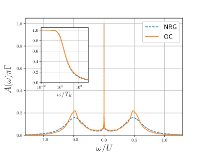
Figure 1: Spectral function $A(\omega)$ in dimensionless units $\omega/U$ for a particle-hole symmetric SIAM with $U/\Gamma=20$, $D/\Gamma=100$ for $T/T_{\rm K}=5.75\cdot 10^{–3}$ and a Kondo temperature of $T_{\rm K}/\Gamma=5.50\cdot 10^{–4}$. The NRG parameters are $\Lambda=2$, $N_{s}=1000$ and $N=50$. A z-averaging with $N_{z}=12$ has been performed. The solid line represents our hybrid open chain (OC) approach without artificial broadening, the dashed line shows the conventional NRG result with a Gaussian broadening parameter $b=0.5$ - see the literature [34, 35, 29] for details. The inset shows the Kondo resonance.

III.2 Spectral function

III.2.1 Results for the spectral function of the symmetric SIAM

We present a comparison of results obtained by the standard NRG approach [34, 35, 29] with the usual artificial broadening (blue, dashed line) and our BR based approach which does not require such additional assumptions (orange solid line). The solid line has been obtained after replacing the expression

$$\rho^{B,\rm red}_{s,r}(m,t=0) = \sum_{s^{\prime}}\left[B_{s,s^{\prime}}(m)\rho^{\rm red}_{s^{\prime},r}(m)\right.$$

$$\phantom{\sum_{s^{\prime}}}-\left.s\rho_{s,s^{\prime}}^{\rm red}(m)B_{s^{\prime},r}(m)\right]$$

on the right hand side of Eq. (37) by its time dependent BR solution $\rho^{B,\rm red}_{s,r}(m,t)$ and analytically performing the Fourier transformation. Note that no artificial broadening was needed.

Figure 1 shows the different spectral functions

$$A_{\sigma}(\omega)=\rho_{d_{\sigma},d^{\dagger}_{\sigma}}(\omega)=-\frac{1}{\pi}\Im G_{d_{\sigma},d^{\dagger}_{\sigma}}(\omega-i\delta)$$ (58)

obtained for a particle-hole symmetric SIAM with $U/\Gamma=20$ and a featureless conduction band, $\Im\Delta(\omega-i\delta)=\Gamma\Theta(D-|\omega|)$, where $D/\Gamma=100$. Since we consider no external magnetic field, i. e. $H=0$, we define $A(\omega)=A_{\sigma}(\omega)$ for both spins $\sigma\in\{\uparrow,\downarrow\}$. The effective temperature of the system is $T/T_{\rm K}=5.75\cdot 10^{–3}$ with a Kondo temperature of $T_{\rm K}/\Gamma=5.50\cdot 10^{–4}$. Throughout the paper, we used Wilson’s definition [28] of $T_{\rm K}$, i. e. $\mu_{\rm eff}^{2}(T_{\rm K})=0.07$, where the effective moment $\mu_{\rm eff}^{2}(T)=T\chi_{\rm imp}(T)$ is linked to the impurity spin susceptibility $\chi_{\rm imp}(T)$ [29].

Since even the standard NRG raw spectral function depends on the artificial broadening parameter $b$ (see review [29] for the technical details), the NRG spectral function typically presented in the literature is obtained from the Dyson equation Eq. (55). In this equation, the self-energy correction $\Sigma^{U}_{\sigma}(z)$ stated in Eq. (56) enters. The effect of the broadening partially cancels [51]. For this reason we calculated the required NRG GFs to obtain $\Sigma^{U}_{\sigma}(z)$ in all approaches and use this $\Sigma^{U}_{\sigma}(z)$ in Eq. (55) for obtaining the final spectrum.

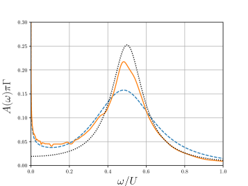
Figure 2: Spectral function $A(\omega)$ in dimensionless units $\omega/U$. Parameters and color coding are identical to Fig. 1. The solid lines represent our hybrid OC approach without artificial broadening, the dashed lines show the conventional NRG result with a Gaussian broadening parameter $b=0.5$. The black dashed line is a fit for the $U/\Gamma\to\infty$ Hubbard-peak at $\omega=U/2$.

Figure 2 focuses on the Hubbard-peak for $\omega>0$ and depicts the same data as in Fig. 1. In the large $U$ limit, an analytic calculation predicts a Lorentzian shape with a width of $2\Gamma$, added to the plot as a black dashed curve. For an calculation of the well known width $2\Gamma$ of the SIAM see Appendix A. The standard NRG approach (dashed blue line) generates a well-known over-broadening [54]. While the raw NRG spectrum is even broader (not shown), the application of Eq. (55) leads to a narrowing that is still significantly too wide at high energies. The BRA (orange solid line) further reduces the over-broadening of the Hubbard-peak. We would like to point out that the structures of the Hubbard peaks also visible in Fig. 1 are an artefact of the approach and dependents on $N_{s}$, $\Lambda$ and also on the number of $z$-values included in the averaging procedure. The width of the Hubbard peaks obtained with the standard approach [34, 35] also converges to $2\Gamma$ but requires a very large number of $N_{z}\gg 100$ combined with an adequately adjusted artificial broadening parameter $b$. This procedure was used [56] to reveal the sharp electron-phonon peaks in the Holstein model at large electron phonon coupling where we choose $N_{z}=512$ and $b=0.03$.

By reducing the discretization parameter $\Lambda\to 1^{+}$ the curve further converges to the analytic prediction (not shown).

III.2.2 Impact of the z-averaging

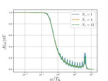
Figure 3: Spectral function $A(\omega)$ in dimensionless units $\omega/T_{\text{K}}$ with a logarithmic horizontal axis. Parameters are identical to Fig. 1. The solid lines represent our hybrid approach without artificial broadening, the dashed lines show the conventional NRG result with a Gaussian broadening parameter $b=0.5$. The effect of z-averaging is shown by variation of the number $N_{z}$ of configurations.

The data in Fig. 1 and  2, was obtained by averaging over $N_{z}=12$ different $z$ values [55, 36, 37] in the NRG. The necessity of z-averaging is illustrated in Fig. 3. Since the BRA only includes the reservoir coupling in second order (see Sec. II.2.) the line width of the NRG exciations acquired from the BRT turns out to be too small. This effectively results in unphysical oscillations of the spectral function curves as depicted in the blue curve for $N_{z}=1$, i. e. in the absence of z-averaging. Varying the $z$-values in the Wilson chain between $0<z\leq 1$ continuously shifts the excitation spectrum of the conduction band tight-binding model. Averaging over several NRG runs for different z-values [55] can smooth these oscillations ($N_{z}>1$ curves of Fig. 3). Here the BR curves basically align with the artificially broadened ones. For $N_{z}=12$ this smoothing effect has basically reached its limit and no significant improvement can be observed by increasing $N_{z}$. To further compensate for the weak coupling of the reservoirs in second order, one would need to decrease $\Lambda$, as discussed above. An extension of the BRA to fourth order coupling is another option to improve the spectrum, yet it does not appear to be feasible from our current point of view - at least if no additional symmetries, such as a diagonal BRT, are considered.

Although the BR equations of the composite operator needed for the calculation of the spectral functions are independent of each other for different $z$-values, and we only include matrix elements within each shell, the computational effort to determine $R_{r_{1},r_{2};r_{3},r_{4}}(m)$ scales roughly as $O(m(4N_{s})^{4})$: The larger the iteration index $m$ the more additional reservoirs have to be included into the tensor elements when evaluating Eqs. (41). The smaller $\Lambda$is, the more NRG states $N_{s}$ must be kept after each iteration [29] to justify the discarding of the high energy states. On the other hand, the spectral weight of the auxiliary reservoir couplings is reduced when reducing $\Lambda$ [30]. This implies that for smaller $\Lambda$ more NRG states contribute to the spectrum with higher energy resolution. Due to the scaling of the BRT calculation with $N_{s}$, this would become numerically extremely expensive so we present a compromise between a practical CPU run-time and a reasonable accuracy of the calculation to prove the usefulness of the approach leaving a better optimized implementation of the algorithm to the future.

We restrict ourselves to the case of low $T\leq 0.01\Gamma$ and, therefore, considerably long Wilson chains of $N=50$ as explained in Sec. II.5, and we can thus assume the off-diagonal elements of the BRT to be irrelevant. This improves the efficiency of the method, since we can apply Eq. (44) in this case . To put the gain in speed into perspective, we have calculated the spectral function for the non-interacting case and without z-averaging (not shown). We treat energies as degenerate if $|E^{m}_{r}-E^{m}_{s}|\leq 10^{-15}\Gamma$. In this case, the deviations of the spectral functions between the approaches with and without off-diagonal elements of the BRT are below $10^{-6}\Gamma^{-1}$ within the interval $|\omega|<10^{-5}\Gamma$ for a temperature $T\approx 10^{-6}\Gamma$. The diagonal approximation reduced program runtime by a factor of $6$.

III.2.3 Finite external magnetic field

(a)

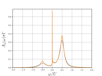
(b)

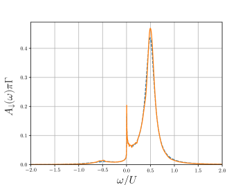
Figure 4: Spectral function $A(\omega)$ of the minority spin in dimensionless units vs $\omega/U$ a in a magnetic field of (a) $H/T_{\text{K}}=5$ and (b) $H/T_{\text{K}}=100$, respectively. Parameters and color coding as Fig. 1.

(a)

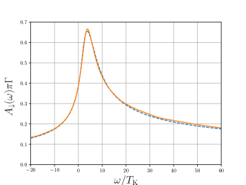
(b)

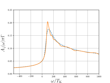
Figure 5: Data of Fig 4 plotted vs $\omega/T_{\text{K}}$, (a) $H/T_{\text{K}}=5$ and (b) $H/T_{\text{K}}=100$. Parameters and color coding as Fig. 1.

In Fig. 4 we present the minority spin spectral function versus $\omega/U$ at a finite magnetic field $H/T_{\text{K}}=5$ and $H/T_{\text{K}}=100$, respectively, for the model parameters of Fig. 1. Note that for a particle-hole symmetric model considered here $A_{\uparrow}(\omega)=A_{\downarrow}(-\omega)$ holds. Therefore, it is sufficient to show only one of the two spectra since they are symmetry related. All other parameters and color coding are identical to those in Fig. 1. A reminiscence of the zero-frequency Kondo resonance with a reduced peak height is still visible. In addition, spectral weight is shifted from the Hubbard peak at $\omega\approx-U/2$ to $\omega\approx U/2$ [58]. For $H/T_{\text{K}}=100$, the lower Hubbard peak is almost completely absent. Regardless of the magnetic field strength, the peaks are sharper in the open chain case.

Using the same data as depicted in Fig. 4, Fig. 5 focuses on the details of the evolution of the Kondo-resonance in a finite magnetic field. The minority spin resonance is shifted to higher energies. At moderate fields, the difference between the standard NRG approach and our open-chain BRA is insignificant. However, within large fields, $H/T_{\text{K}}=100$, the asymmetry becomes more pronounced and the BR spectrum is much sharper around the excitation threshold of $\omega\approx H$. [59, 60].

IV Conclusion

We presented an approach to spectral functions of QISs that eliminates the requirement for an artificial broadening of the Lehmann representation due to the discretization of the QIS. The starting point was the exact representation of the original bath coupling function by a Wilson chain augmented with a set of high-energy reservoirs [31, 30]. By adapting the BRA [38, 39] to GFs based on the recently presented open chain TD-NRG approach [30] we are able to include life-time effects on the NRG excitations induced by bath coupling which is neglected in the pure Wilson chain.

Since the approach is based on the complete basis for the Wilson chain [36, 37], the spectral sum-rules are always exactly fulfilled, independent of the number $N_{s}$ of kept states after each NRG iteration and independent of the new decay channels introduced by the additional reservoirs.

By combining our BRA to GFs with z-averaging and the exact relations obtained from the equation of motion [51] we obtain very accurate spectral functions from the NRG without further broadening parameters. We gauged the quality of our spectra for $T\to 0$ with the results of a standard NRG approach [34]. Our approach tracks the low energy Kondo-resonance very accurately and produces high energy Hubbard peaks that are much narrower that the standard NRG spectrum: Our artificial broadening free open-chain spectra approach the analytic prediction of a Lorentzian of width $2\Gamma$ [61] for large $U$.

We also presented spectra in a finite magnetic field. While for small fields, i. e. $H\approx T_{\text{K}}$, the open chain approach essentially agrees with the standard NRG results, significant deviations are observed for $H/T_{\text{K}}>50$: the spectral properties become much sharper and much more pronounced around $\omega\approx\pm H$ and slowly approach the analytic predictions [59] for the Kondo model in very large fields.

Although our approach is tailored towards the partitioning of the NRG eigenbasis, the general strategy can readily be adapted to other discretized representations of QISs such as the ED and the D-DMRG [25, 26, 27]. For the D-DMRG the hybridization function is typically treated by a continuous fraction expansion [40] producing a finite tight-binding chain augmented by a single reservoir at the end of the chain that is omitted in the standard method. In contrast to the Wilson chain, for this tight-binding case the dynamics of the composite operator $\hat{\rho}^{I}_{B,{S}}(t)$ as stated in Eq. (12) still hold, but the reservoir coupling functions vanish with the exception of the last chain site $\tilde{m}=N$. In ED and in the D-DMRG one might proceed in constructing a suitable Krylov space by applying the Hamiltonian onto a starting vector suitable for the GF of interest and calculate the dynamics of the operator $\rho^{I}_{B,{S}}(t)$ in this reduced Krylov space [41] to include life-time effects of the reservoirs neglected in the conventional approaches.

V Acknowledgments

We acknowledge fruitful discussions with Jan von Delft and Saurabh Pradhan, and financial support by Deutsche Forschungsgemeinschaft via the Grant No. AN 275/10-1.

Appendix A Simple example: Spectral function of the SIAM

Let us consider the minimal Hamiltonian for $H_{S}$ in the SIAM,

$$H_{S} = H_{\text{imp}}=\sum_{\sigma}\epsilon_{d\sigma}d^{\dagger}_{\sigma}d_{\sigma}+Un_{\uparrow}n_{\downarrow}$$ (59)

and treat the full bath continuum of the SIAM by the BRA. The four eigenstates $|\alpha\rangle$ with $\alpha=0,\sigma,2$ span a four dimensional Fock space of the impurity. The Hubbard operators $X_{\alpha,\beta}=|\alpha\rangle\langle\beta|$ mediate transitions from the local state $|\beta\rangle$ to the state $|\alpha\rangle$. We also omit the external magnetic field and, therefore, set $\epsilon_{d\sigma}=\epsilon_{d}$. Since the Kondo effect is caused by an entanglement between the impurity states and the conduction band continuum, no Kondo resonance can be found within this approximation.

For the local GF $G_{d_{\sigma},d^{\dagger}_{\sigma}}(z)$, the initial composite operator, $\hat{\rho}_{B,{S}}^{I}(t=0)$, is given by

$$\hat{\rho}_{B,S}^{I}(0) = d^{\dagger}_{\sigma}\hat{\rho}_{S}+\hat{\rho}_{S}d^{\dagger}_{\sigma}$$ (60)

$$= X_{\sigma,0}(\rho_{0,0}+\rho_{\sigma,\sigma})-\sigma X_{2,-\sigma}(\rho_{-\sigma,-\sigma}+\rho_{2,2})$$

$$= X_{\sigma,0}A_{\sigma,0}-\sigma X_{2,-\sigma}B_{2,-\sigma},$$

where $\rho_{i,j}$ are the matrix elements of $\hat{\rho}_{S}$. This reduced density operator transforms as a local fermionic creation operator and can be used to evaluate

$${\rm Tr}\left[d_{\sigma}\hat{\rho}_{B}(t)\right] ={\rm Tr}_{S}\left[d_{\sigma}e^{-iH_{S}t}\hat{\rho}_{B,{S}}^{I}(t)e^{iH_{S}t}\right]$$ (61)

$$=e^{i(E_{0}-E_{\sigma})t}A_{\sigma,0}(t)-\sigma e^{i(E_{-\sigma}-E_{2})t}B_{2,-\sigma}(t).$$

The time dependent matrix elements $A_{\sigma,0}(t)=\langle\sigma|\hat{\rho}_{B,{S}}^{I}(t)|0\rangle$ and $B_{2,-\sigma}(t)=\langle 2|\hat{\rho}_{B,{S}}^{I}(t)|-\sigma\rangle$ contain the information about the operator decay caused by the coupling to the reservoirs. Apparently, we need to distinguish two cases: if both excitation energies, $E_{0}-E_{\sigma}$ and $E_{-\sigma}-E_{2}$, respectively, are equal, then the exponential prefactor can be pulled out, and we are left with a combined dynamics of $A_{\sigma,0}(t)-\sigma B_{2,-\sigma}(t)$, whose initial condition is given by $A_{\sigma,0}(0)-\sigma B_{2,-\sigma}(0)=1$. This is the case for $U=0$, indicating that different density matrix elements corresponding to the same excitation energy are coupled by Eq. (41).

For finite $U$ both excitation energies are different. In this case, the matrix elements decouple and we find the solutions

$$A_{\sigma,0}(t) = e^{-tR_{\sigma,0;\sigma,0}}A_{\sigma,0}(0)$$ (62)

$$B_{2,-\sigma}(t) = e^{-tR_{2,-\sigma;2,-\sigma}}B_{2,-\sigma}(0)$$ (63)

which leaves us to calculate the BRT elements.

We focus on the regime where $E_{\sigma}<E_{2},E_{0}$, and, therefore, local moments can develop. In this case, the correct solution would show a Kondo resonance that must be absent in this perturbative approach. At low temperatures, i. e., $|\beta\epsilon_{d}|\gg 1$ we find for a constant hybridization function in a symmetric band of width $D\gg|\epsilon_{d}|$

$$R_{\sigma,0;\sigma,0} = 2\Gamma+i2\Delta E,$$ (64)

where the Lamb shift in the presence of the continuum is given by

$$\Delta E = \frac{\Gamma}{\pi}\ln\left(\frac{|D+\epsilon_{d}|}{|\epsilon_{d}|}\right)$$ (65)

Likewise,

$$R_{2,-\sigma,2,-\sigma} = 2\Gamma-i2\Delta\bar{E}$$ (66)

$$\Delta\bar{E} = \frac{\Gamma}{\pi}\ln\left(\frac{|D-(\epsilon_{d}+U)|}{|\epsilon_{d}+U|}\right)$$ (67)

Substituting these analytic solutions back into Eq. (II.4) or even Eq. (6), calculating the trace and performing the Fourier transformations leads to two contributing decaying poles

$$G^{\text{r}}_{d_{\sigma},d^{\dagger}_{\sigma}}(\omega+i\delta) = \frac{A_{\sigma,0}(0)}{\omega+i\delta-\epsilon_{d}-2\Delta E+i2\Gamma}$$

$$+\frac{B_{2,-\sigma}(0)}{\omega+i\delta-(\epsilon_{d}+U)+2\Delta\bar{E}+i2\Gamma}.$$

For a particle-hole symmetric impurity we have $\Delta\bar{E}=\Delta E$ since $\epsilon_{d}=-(\epsilon_{d}+U)$, and, therefore, both poles are shifted symmetrically by the Lamb-shift $\Delta E$. The fractional spectral weights are also symmetric and add up to $1$. Note that the width of the excitations is given by $2\Gamma$ which agrees with the analytical prediction by Grewe [61].

For $U=0$ one has to be more careful when evaluating the rate equation (41). Since the two excitation energies $E_{\sigma,0}=E_{2,-\sigma}=\epsilon_{d}$ are equal, the two matrix elements $\rho^{B}_{\sigma,0}$ and $\rho^{B}_{2,-\sigma}$ are coupled. The differential equation for $A_{\sigma,0}(t)-\sigma B_{2,-\sigma}(t)$ is rather simple and is derived from the dynamics of $A_{\sigma,0}(t)$ and $B_{2,-\sigma}(t)$. For a constant density of states, it is straight forward to show that we recover the exact GF

$$G^{\text{r}}_{d_{\sigma},d^{\dagger}_{\sigma}}(\omega+i\delta) = \frac{1}{\omega+i\delta-\epsilon_{d}+\delta E+i\Gamma}$$ (69)

where

$$\delta E=\frac{\Gamma}{\pi}\ln\left|\frac{D-\epsilon_{\text{d}}}{D+\epsilon_{\text{d}}}\right|$$ (70)

is the known contribution from the real part of the self-energy. Note that the width of the GF is reduced to $\Gamma$, compared to $2\Gamma$ in the case of a finite $U$. The reduction originates in the negative sign of the term including $B_{2,-\sigma}(t)$, which enters the calculation of the GFs. In the combined differential equations there is a compensation of different terms contributing to the individual BRT elements defined in Eq. (42).

This leaves the question what causes the discontinuity between the solutions for $U=0$ and for $U\not=0$. This discontinuity is related to the secular approximation. When $U\ll\Gamma$, the approximation does not hold since the excitation energies are small compared to the inverse time scale of the decay of the correlation functions. In this case, we have to resort to a full time dependence in Eq. (12). In the particle-hole symmetric case, one can show [47] that this leads to the integro-differential equation

$$\dot{A}_{\sigma,0}(t) = -\frac{2\Gamma}{\pi}\int_{0}^{t}ds\frac{\sin(Ds)}{s}e^{-iUs/2}$$

$$\times\left[2A_{\sigma,0}(t)-e^{-iU(t-s)}A^{*}_{\sigma,0}(t)\right]$$

where $A_{\sigma,0}(t)=B^{*}_{2,-\sigma}(t)$.

Extending the local system to a small but finite Wilson chain removes the discontinuity at $U=0$ in the spectral functions obtained in the secular approximation. For more details see Ref. [47].

References

- Anderson [1961] P. W. Anderson, Localized Magnetic States in Metals, Phys. Rev. 124, 41 (1961).
- Kondo [1964] J. Kondo, Resistance minimum in dilute magnetic alloys, Progress of Theoretical Physics 32, 37 (1964).
- Krishna-murthy et al. [1980a] H. R. Krishna-murthy, J. W. Wilkins, and K. G. Wilson, Renormalization-group approach to the Anderson model of dilute magnetic alloys. I. Static properties for the symmetric case, Phys. Rev. B 21, 1003 (1980a).
- Krishna-murthy et al. [1980b] H. R. Krishna-murthy, J. W. Wilkins, and K. G. Wilson, Renormalization-group approach to the Anderson model of dilute magnetic alloys. II. Static properties for the asymmetric case, Phys. Rev. B 21, 1044 (1980b).
- Kuramoto [1985] Y. Kuramoto, in Theory of Heavy Fermions and Valence Fluctuations, edited by T. Kasuya and T. Saso (Springer Verlag, Berlin, 1985) p. 152.
- Georges et al. [1996] A. Georges, G. Kotliar, W. Krauth, and M. J. Rozenberg, Dynamical mean-field theory of strongly correlated fermion systems and the limit of infinite dimensions, Rev. Mod. Phys. 68, 13 (1996).
- Kotliar and Vollhardt [2004] G. Kotliar and D. Vollhardt, Strongly correlated materials: Insights from dynamical mean field theory, Physics Today 57, 53 (2004).
- Kastner [1992] M. A. Kastner, The single-electron transistor, Rev. Mod. Phys. 64, 849 (1992).
- Goldhaber-Gordon et al. [1998a] D. Goldhaber-Gordon, H. Shtrikman, D. Mahalu, D. Abusch-Magder, U. Meirav, and M. Kastner, Kondo effect in a single-electron transistor, Nature 391, 156 (1998a).
- Goldhaber-Gordon et al. [1998b] D. Goldhaber-Gordon, J. Göres, M. A. Kastner, H. Shtrikman, D. Mahalu, and U. Meirav, From the kondo regime to the mixed-valence regime in a single-electron transistor, Phys. Rev. Lett. 81, 5225 (1998b).
- van der Wiel et al. [2000] W. G. van der Wiel, S. D. Franceschi, T. F. J. Elzerman, S. Tarucha, and L. P. Kouvenhoven, The kondo effect in the unitary limit, Science 289, 2105 (2000).
- Manoharan et al. [2000] H. C. Manoharan, C. P. Lutz, and D. M. Eigler, Quantum mirages formed by coherent projection of electronic structure, Nature 403, 512 (2000).
- Agam and Schiller [2001] O. Agam and A. Schiller, Projecting the kondo effect: Theory of the quantum mirage, Phys. Rev. Lett. 86, 484 (2001).
- Galperin et al. [2006] M. Galperin, A. Nitzan, and M. A. Ratner, Molecular transport junctions: Current from electronic excitations in the leads, Physical Review Letters 96, 166803 (2006).
- Heath [2009] J. R. Heath, Molecular electronics, Annual Review of Materials Research 39, 1 (2009).
- Lorente and Persson [2000] N. Lorente and M. Persson, Theory of single molecule vibrational spectroscopy and microscopy, Phys. Rev. Lett. 85, 2997 (2000).
- Reed [2008] M. A. Reed, Inelastic electron tunneling spectroscopy, Materials Today 11, 46 (2008).
- Eickhoff et al. [2020] F. Eickhoff, E. Kolodzeiski, T. Esat, N. Fournier, C. Wagner, T. Deilmann, R. Temirov, M. Rohlfing, F. S. Tautz, and F. B. Anders, Inelastic electron tunneling spectroscopy for probing strongly correlated many-body systems by scanning tunneling microscopy, Phys. Rev. B 101, 125405 (2020).
- Pereira et al. [2006] V. M. Pereira, F. Guinea, J. M. B. Lopes dos Santos, N. M. R. Peres, and A. H. Castro Neto, Disorder induced localized states in graphene, Phys. Rev. Let. 96, 036801 (2006).
- Cazalilla et al. [2012] M. A. Cazalilla, A. Iucci, F. Guinea, and A. H. C. Neto, Local moment formation and kondo effect in defective graphene, arXiv: 1207.3135 (2012).
- May et al. [2018] D. May, P.-W. Lo, K. Deltenre, A. Henke, J. Mao, Y. Jiang, G. Li, E. Y. Andrei, G.-Y. Guo, and F. B. Anders, Modeling of the gate-controlled Kondo effect at carbon point defects in Graphene, Phys. Rev. B 97, 155419 (2018).
- Jiang et al. [2018] Y. Jiang, P.-W. Lo, D. May, G. Li, G.-Y. Guo, F. B. Anders, T. Taniguchi, K. Watanabe, J. Mao, and E. Y. Andrei, Inducing kondo screening of vacancy magnetic moments in graphene with gating and local curvature, Nature Communications 9, 2349 (2018).
- Esat et al. [2016] T. Esat, B. Lechtenberg, T. Deilmann, ChristianWagner, P. Krüger, R. Temirov, M. Rohlfing, F. B. Anders, and F. S. Tautz, A chemically driven quantum phase transition in a two-molecule Kondo system, Nature Physics 12, 867 (2016).
- Caffarel and Krauth [1994] M. Caffarel and W. Krauth, Exact diagonalization approach to correlated fermions in infinite dimensions: Mott transition and superconductivity, Phys. Rev. Lett. 72, 1545 (1994).
- White [1992] S. White, Density matrix formulation for quantum renormalization groups, Phys. Rev. Lett. 69, 2863 (1992).
- Schollwöck [2005] U. Schollwöck, The density-matrix renormalization group, Rev. Mod. Phys. 77, 259 (2005).
- Schollwöck [2011] U. Schollwöck, The density-matrix renormalization group in the age of matrix product states, Ann. Phys. (Amsterdam) 326, 96 (2011).
- Wilson [1975] K. G. Wilson, Rev. Mod. Phys. 47, 773 (1975).
- Bulla et al. [2008] R. Bulla, T. A. Costi, and T. Pruschke, The numerical renormalization group method for quantum impurity systems, Rev. Mod. Phys. 80, 395 (2008).
- Böker and Anders [2020] J. Böker and F. B. Anders, Restoring the continuum limit in the time-dependent numerical renormalization group approach, Phys. Rev. B 102, 075149 (2020).
- Bruognolo et al. [2017] B. Bruognolo, N.-O. Linden, F. Schwarz, S.-S. B. Lee, K. Stadler, A. Weichselbaum, M. Vojta, F. B. Anders, and J. von Delft, Open wilson chains for quantum impurity models: Keeping track of all bath modes, Phys. Rev. B 95, 121115 (2017).
- Leggett et al. [1987] A. J. Leggett, S. Chakravarty, A. T. Dorsey, and M. P. A. Fisher, Dynamics of the dissipative two-state system, Rev. Mod. Phys. 59, 1 (1987).
- Vojta et al. [2010] M. Vojta, R. Bulla, F. Guettge, and F. Anders, The mass-flow error in the Numerical Renormalization Group method and the critical behavior of the sub-ohmic spin-boson model, Physical Review B 81, 075122 (2010).
- Peters et al. [2006] R. Peters, T. Pruschke, and F. B. Anders, A numerical renormalization group approach to green’s functions for quantum impurity models, Phys. Rev. B 74, 245114 (2006).
- Weichselbaum and von Delft [2007] A. Weichselbaum and J. von Delft, Sum-rule conserving spectral functions from the numerical renormalization group, Phys. Rev. Lett. 99, 076402 (2007).
- Anders and Schiller [2005] F. B. Anders and A. Schiller, Time-dependent numerical renormalization group approach to non-equilibrium dynamics of quantum impurity systems, Phys. Rev. Lett. 95, 196801 (2005).
- Anders and Schiller [2006] F. B. Anders and A. Schiller, Spin precession and real-time dynamics in the kondo model: Time-dependent numerical renormalization-group study, Phys. Rev. B 74, 245113 (2006).
- May and Kühn [2000] V. May and O. Kühn, Charge and Energy Transfer Dynamics in Molecular Systems (Wiley-VCH, Berlin, 2000).
- Jeske et al. [2015] J. Jeske, D. J. Ing, M. B. Plenio, S. F. Huelga, and J. H. Cole, Bloch-redfield equations for modeling light-harvesting complexes, The Journal of Chemical Physics 142, 064104 (2015).
- Raas et al. [2004] C. Raas, G. S. Uhrig, and F. B. Anders, High energy dynamics of the single impurity anderson model, Phys. Rev. B 69, 041102 (2004).
- Nocera and Alvarez [2016] A. Nocera and G. Alvarez, Spectral functions with the density matrix renormalization group: Krylov-space approach for correction vectors, Phys. Rev. E 94, 053308 (2016).
- Carmichael [1999] H. J. Carmichael, Statistical Methods in Quantum Optics 1 (Springer Verlag, Berlin Heidelberg, 1999).
- Dzhioev and Kosov [2012] A. A. Dzhioev and D. S. Kosov, Nonequilibrium perturbation theory in liouville–fock space for inelastic electron transport, Journal of Physics: Condensed Matter 24, 225304 (2012).
- Dorda et al. [2015] A. Dorda, M. Ganahl, H. G. Evertz, W. von der Linden, and E. Arrigoni, Auxiliary master equation approach within matrix product states: Spectral properties of the nonequilibrium anderson impurity model, Phys. Rev. B 92, 125145 (2015).
- Schwarz et al. [2016] F. Schwarz, M. Goldstein, A. Dorda, E. Arrigoni, A. Weichselbaum, and J. von Delft, Lindblad-driven discretized leads for nonequilibrium steady-state transport in quantum impurity models: Recovering the continuum limit, Phys. Rev. B 94, 155142 (2016).
- Bulla et al. [1997] R. Bulla, T. Pruschke, and A. C. Hewson, Anderson impurity in pseudo-gap fermi systems, Journal of Physics: Condensed Matter 9, 10463 (1997).
- Boeker [2021] J. O. Boeker, A Novel Hybrid Numerical Renormalization Group Approach to Non-Equilibrium Dynamics and Spectral Functions, Ph.D. thesis, TU Dortmund university, 44221 Dortmund, Germany (2021).
- Saad [2003] Y. Saad, Iterative Methods for Sparse Linear Systems, (Society for Industrial and Applied Mathematics, Philadelphia, USA, 2003).
- Schlottmann [1989] P. Schlottmann, Some exact results for dilute mixed-valent and heavy-fermion systems, Physics Reports 181, 1 (1989).
- Andrei et al. [1983] N. Andrei, K. Furuya, and J. H. Lowenstein, Rev. Mod. Phys. 55, 331 (1983).
- Bulla et al. [1998] R. Bulla, A. C. Hewson, and T. Pruschke, Numerical renormalization group calculations for the self-energy of the impurity anderson model, J. Phys.: Condens. Matter 10, 8365 (1998).
- Yamada [1975] K. Yamada, Prog. Theor. Phys. 53, 970 (1975).
- Yamada [1975] K. Yamada, Perturbation expansion for the Anderson hamiltonian. IV, Prog. Theor. Phys. 54, 316 (1975).
- Grewe et al. [2008] N. Grewe, S. Schmitt, T. Jabben, and F. B. Anders, Conserving approximations in direct perturbation theory: new semianalytical impurity solvers and their application to general lattice problems, Journal of Physics: Condensed Matter 20, 365217 (2008).
- Yoshida et al. [1990] M. Yoshida, M. A. Whitaker, and L. N. Oliveira, Renormalization-group calulation of excitation properties for impurity models, Phys. Rev. B 41, 9403 (1990).
- Jovchev and Anders [2013] A. Jovchev and F. B. Anders, Influence of vibrational modes on quantum transport through a nanodevice, Phys. Rev. B 87, 195112 (2013).
- Note [1] We have analytically shown in Appendix A how the off-diagonal BRT elements are needed in the case of the atomic limit, i. e. , to generate the correct line width for .
- Hofstetter [2000] W. Hofstetter, Generalized numerical renormalization group for dynamical quantities, Phys. Rev. Lett. 85, 1508 (2000).
- Rosch et al. [2003] A. Rosch, T. A. Costi, J. Paaske, and P. Wölfle, Spectral function of the kondo model in high magnetic fields, Phys. Rev. B 68, 014430 (2003).
- Schoeller [2009] H. Schoeller, A perturbative nonequilibrium renormalization group method for dissipative quantum mechanics, Eur. Phys. J. Special Topics 168, 179 (2009).
- Grewe [1983] N. Grewe, Z. Phys. B 52, 193 (1983).