Robust Controllers for a Flexible Satellite Model

Abstract.

We consider a PDE-ODE model of a flexible satellite that is composed of two identical flexible solar panels and a center rigid body. We prove that the satellite model is exponentially stable in the sense that the energy of the solutions decays to zero exponentially. In addition, we construct two internal model based controllers, a passive controller and an observer based controller, such that the linear and angular velocities of the center rigid body converge to the given sinusoidal signals asymptotically. A numerical simulation is presented to compare the performances of the two controllers.

1. Introduction

In this paper, we consider output tracking and disturbance rejection problem for a flexible satellite that is composed of two identical flexible solar panels and a center rigid body (Figure 1). Modeling the satellite panels as viscously damped Euler-Bernoulli beams of length 1, the satellite system we study is given by (similar models can be found in [6], [13])

Figure 1. Satellite with flexible solar panels

(1) $$\begin{gathered}\rho a\ddot{w}_{l}(\xi,t)+EIw_{l}^{\prime\prime\prime\prime}(\xi,t)+\gamma\dot{w}_{l}(\xi,t)=b_{d1}(\xi)w_{d1}(t),\ -1<\xi<0,t>0,\\ \rho a\ddot{w}_{r}(\xi,t)+EIw_{r}^{\prime\prime\prime\prime}(\xi,t)+\gamma\dot{w}_{r}(\xi,t)=b_{d2}(\xi)w_{d2}(t),\ 0<\xi<1,t>0,\\ m\ddot{w}_{c}(t)=EIw_{l}^{\prime\prime\prime}(0,t)-EIw_{r}^{\prime\prime\prime}(0,t)+u_{1}(t)+w_{d3}(t),\\ I_{m}\ddot{\theta}_{c}(t)=-EIw_{l}^{\prime\prime}(0,t)+EIw_{r}^{\prime\prime}(0,t)+u_{2}(t)+w_{d4}(t),\\ w_{l}^{\prime\prime}(-1,t)=0,\quad\ w_{l}^{\prime\prime\prime}(-1,t)=0,\\ w_{r}^{\prime\prime}(1,t)=0,\quad\ w_{r}^{\prime\prime\prime}(1,t)=0,\\ \dot{w}_{l}(0,t)=\dot{w}_{r}(0,t)=\dot{w_{c}}(t),\\ \dot{w}_{l}^{\prime}(0,t)=\dot{w}_{r}^{\prime}(0,t)=\dot{\theta}_{c}(t),\end{gathered}$$

where $w_{l}(\xi,t)$ and $w_{r}(\xi,t)$ are the transverse displacements of the left and the right beam, respectively, $\dot{w}_{l}(\xi,t)$ and $w_{l}^{\prime}(\xi,t)$ denote time and spatial derivatives of $w_{l}(\xi,t)$, respectively, $w_{c}(t)$ and $\theta_{c}(t)$ are the linear and angular displacements of the rigid body, respectively, $u_{1}(t)$ and $u_{2}(t)$ are external control inputs of the satellite model, $w_{d1}(t)$, $w_{d2}(t)$, $w_{d3}(t)$ and $w_{d4}(t)$ are external disturbances in the satellite model, $b_{d1}(\cdot)\in L^{2}(-1,0)$ and $b_{d2}(\cdot)\in L^{2}(0,1)$ are real-valued functions. Here $\dot{w}_{c}(t)=\dot{w}_{l}(\xi,t)|_{\xi=0}=\dot{w}_{r}(\xi,t)|_{\xi=0}$ and $\dot{\theta}_{c}(t)=\dot{w}_{l}^{\prime}(\xi,t)|_{\xi=0}=\dot{w}_{r}^{\prime}(\xi,t)|_{\xi=0}$ are linear and angular velocities of the rigid body, respectively. The parameters $a$, $\rho$, $E$, $I$ and $\gamma$ are cross sectional area, linear density, Young’s modulus of elasticity, second moment of area of the cross section and the viscous damping coefficient of the beams, respectively, and $m$ and $I_{m}$ denote the mass and the mass moment of inertia of the center rigid body. Measurements that are the outputs of the model are taken on the center rigid body and are given by,

(2) $$y_{1}(t)=\dot{w}_{c}(t),\ y_{2}(t)=\dot{\theta}_{c}(t).$$

The main control objective is to construct a dynamic error feedback controller such that the outputs, the linear and the angular velocities of the center rigid body, track given reference signals $y_{ref}(t)$ asymptotically. i.e.,

$$\lVert y(t)-y_{ref}(t)\rVert\rightarrow 0\quad\text{as}\quad t\rightarrow\infty,$$

where $y(t)=(y_{1}(t),y_{2}(t))^{T}$ is the output of the satellite model. In addition, the proposed controller is required to be robust in the sense that it achieves output tracking despite perturbations, disturbances and uncertainties in the satellite system.

As the first main contribution of this paper, we present a detailed proof of uniform exponential stability of the satellite model in the sense that the energy of the solutions decay exponentially to zero. The stability proof is based on the results from $C_{0}$-semigroup theory. We write the satellite system as a coupled system of a PDE (two beams are combined into a single system) and an ODE (rigid body) via a power preserving interconnection. The main proof is divided naturally into two steps. In the first step, we show that the imaginary axis is included in the resolvent set of the satellite system operator. In the second step, we derive an explicit expression for the resolvent operator and show that it is uniformly bounded on the imaginary axis. The stability proof is challenging because the input and the output operators of the PDE are not admissible and its transfer function is not well-posed (in the sense that the input-output map of the PDE is unbounded).

As the second main contribution of this paper, we construct two robust controllers, a passive controller [20], [18] and an observer based controller [12], [17], for the robust output tracking of the satellite model. The proposed controller designs are based on the internal model principle [9], [10], [12], [17], [19]. Finally, simulation results testing the effectiveness of the controllers are presented.

There are several studies in the literature investigating control problems of satellite models. In [6], the stabilization problem of a flexible spacecraft has been investigated using frequency domain approach. In [13], dynamic modeling and vibration control of a flexible satellite has been considered and vibrations of the solar panels have been suppressed using the single-point control input on the center body. In [1], modeling and control of a rotating flexible spacecraft has been considered, a Proportional Derivative controller and a nonlinear controller have been presented to suppress elastic vibrations of the satellite model. References [13] and [1] use Lyapunov methods to prove the stability of the models. To the best of our knowledge, robust output tracking problem for flexible satellites has not been considered in the literature.

Stability of coupled PDE-ODE systems can often be obtained using controllability and observability results. In [24], controllability and observability results of a well-posed and strictly proper linear system coupled with a finite-dimensional linear system with an invertible first component in its feedthrough matrix were presented. In [25], using results from [24], strong stability of coupled impedance passive systems was shown and the results were applied to the SCOLE model to show that the SCOLE model coupled with tuned mass damper system is strongly stable. Moreover, the SCOLE model is not exactly controllable in the natural energy state space ([22, Sec. 1]) but it was shown in [22] that the SCOLE model is exactly controllable in a smoother state space. In [23], it was shown that a coupled system consisting of a well-posed and impedance passive linear system and an internal model based controller in a feedback connection is strongly stable. In our case, since the beam system in the satellite model is not well-posed on the natural energy state space and the rigid center body has no feedthrough term, the results of [24], [25] cannot be utilized in showing the exponential stability of the satellite system. Moreover, since our aim is to achieve exponential stability of the closed-loop system and one of the proposed controllers is infinite-dimensional, the results in [22], [24], [25] and [23] are not applicable in showing the exponential stability of the closed-loop system consisting of the satellite system and the controller. The results in the above mentioned references have unstable infinite-dimensional part and therefore only strong stability of the coupled system was obtained. In this work, since the beam system is exponentially stable due to the distributed damping, we are able to prove the exponential stability of the satellite system.

A preliminary version of these results has been presented in IFAC World Congress 2020 [11]. As the main novelty of this version with respect to [11], we present a detailed proof of the exponential stability of the satellite system. We present a passive controller and an observer based controller which also achieve the robust output tracking of the satellite model and reject external disturbances. In addition, simulation results showing the performances of the controllers are presented.

The paper is organized as follows. In Section 2, we present the abstract formulation of the satellite model. In Section 3, we present some technical lemmas and prove the exponential stability of the satellite model. In Section 4, we present the tracking problem, the reference signal to be tracked by the satellite model and the disturbance signals to be rejected. We present two internal model based controllers for the robust output tracking of the satellite model. In addition, simulation results are presented for particular choices of reference and disturbance signals. In Section 5, we conclude our results.

1.1. Notation

For normed linear spaces $X$ and $Y$, $\mathcal{L}(X,Y)$ denotes the set of bounded linear operators from $X$ to $Y$. For a linear operator $A$, $D(A),\mathcal{R}(A)$ and $\mathcal{N}(A)$ denote domain, range and kernel of $A$, respectively. The resolvent and the spectrum of $A$ are denoted by $\rho(A)$ and $\sigma(A)$, respectively. The resolvent operator is denoted by $R(\lambda,A)=(\lambda-A)^{-1},\ \lambda\in\rho(A)$. We denote by $X_{-1}$ the completion of $X$ with respect to the norm $\|x\|_{-1}=\|(\beta I-A)^{-1}x\|,\ x\in X,\ \beta\in\rho(A)$ and by $A_{-1}\in\mathcal{L}(X,X_{-1})$, the extension of $A$ to $X_{-1}$. For functions $f,g:I\subset\mathbb{R}\to\mathbb{R}_{+}$ and $f_{k},g_{k}\geq 0$, we denote $f(x)\lesssim g(x)$ and $f_{k}\lesssim g_{k}$ if there exist $M_{1},M_{2}>0$ such that $f(x)\leq M_{1}g(x)$ and $f_{k}\leq M_{2}g_{k}$ for all values of $x\in I$ and $k\in J\subset\mathbb{N}$.

2. Abstract Formulation of the Satellite Model

In this section, we write our satellite model (1)-(2) in the state space form

(3) $$\dot{x}(t) =Ax(t)+Bu(t)+B_{d}w_{d}(t),\quad x(0)=x_{0},$$

$$y(t) =Cx(t)$$

where $x(t)\in X$ is the state variable and $X$ is a Hilbert space, $u(t)\in U=\mathbb{R}^{2}$ is the control input, $w_{d}(t)\in U_{d}=\mathbb{R}^{4}$ is the external disturbance and $y(t)\in Y=\mathbb{R}^{2}$ is the output. The operator $A:D(A)\subset X\to X$ generates a strongly continuous semigroup on $X$ and the operators $B\in\mathcal{L}(U,X)$, $B_{d}\in\mathcal{L}(U_{d},X)$ and $C\in\mathcal{L}(X,Y)$ are bounded. The formulation (3) will be used in Section 4 in the construction of controllers for robust output regulation.

In order to write the satellite model (1)-(2) in the state space form, we decompose the satellite system into a PDE system (the two beams combined into a single system) coupled with an ODE system (center rigid body) where PDE interacts with ODE via boundary controls and boundary observations called “virtual boundary inputs” and “virtual boundary outputs”, respectively. Figure 2 shows the boundary interconnections between the beams and the center rigid body. This type of decomposition has been considered, for example, in [22] for SCOLE model.

Figure 2. Coupling of the beams with the rigid body

As the first step towards state space formulation, we write the PDE as an impedance passive abstract boundary control and observation system given by the following definitions.

Definition 2.1 (Boundary Control and Observation System [8, Def. 3.3.2], [14, Ch. 11]).

Let $\hat{X}$, $\hat{U}$ and $\hat{Y}$ be Hilbert spaces. Consider the system

(4a) $$\dot{\hat{x}}(t) =\mathcal{\hat{A}}\hat{x}(t),\quad\hat{x}(0)=\hat{x}_{0},$$

(4b) $$\mathcal{\hat{B}}\hat{x}(t) =\hat{u}(t),$$

(4c) $$\hat{y}(t) =\mathcal{\hat{C}}\hat{x}(t)$$

where $\mathcal{\hat{A}}:D(\mathcal{\hat{A}})\subset\hat{X}\rightarrow\hat{X}$, $\mathcal{\hat{B}}:D(\mathcal{\hat{B}})\subset\hat{X}\rightarrow\hat{U}$ and $\mathcal{\hat{C}}:D(\mathcal{\hat{A}})\rightarrow\hat{Y}$ are linear operators and $D(\mathcal{\hat{A}})\subset D(\mathcal{\hat{B}})$. Then (4) is a boundary control and observation system if the following hold.

1. The operator $\hat{A}:D(\hat{A})\rightarrow\hat{X}$ with $D(\hat{A})=D(\mathcal{\hat{A}})\cap\mathcal{N}(\mathcal{\hat{B}})$ and $\hat{A}\hat{x}=\mathcal{\hat{A}}\hat{x}$ for $\hat{x}\in D(\hat{A})$ is the infinitesimal generator of a $C_{0}$-semigroup $(\hat{T}(t))_{t\geq 0}$ on $\hat{X}$.

2. There exists an operator $\hat{H}\in\mathcal{L}(\hat{U},\hat{X})$ such that for all $\hat{u}\in\hat{U}$ we have $\hat{H}\hat{u}\in D(\mathcal{\hat{A}})$, $\mathcal{\hat{A}}\hat{H}\in\mathcal{L}(\hat{U},\hat{X})$ and $\mathcal{\hat{B}}\hat{H}\hat{u}=\hat{u},\ \hat{u}\in\hat{U}$.

Remark 2.2.

Let $(\mathcal{\hat{A}},\mathcal{\hat{B}})$ be a boundary control system. Then according to [21, Ch. 10], there exists a unique $\hat{B}\in\mathcal{L}(\hat{U},\hat{X}_{-1})$ such that $\mathcal{\hat{A}}=\hat{A}_{-1}+\hat{B}\mathcal{\hat{B}}$ on $D(\mathcal{\hat{A}})$ and therefore (4a) and (4b) can be written as

$$\dot{\hat{x}}(t) =\hat{A}_{-1}\hat{x}(t)+\hat{B}\hat{u}(t),\quad\hat{x}(0)=\hat{x}_{0}.$$

Definition 2.3 (Impedance Passive System).

The system $(\mathcal{\hat{A}},\mathcal{\hat{B}},\mathcal{\hat{C}})$ is called impedance passive if the solutions of (4) satisfy

$$\frac{1}{2}\frac{d}{dt}\lVert\hat{x}(t)\rVert_{\hat{X}}^{2}\leq\text{Re}\left\langle\hat{u}(t),\hat{y}(t)\right\rangle_{\hat{U},\hat{Y}},\quad t>0.$$

We note that the above definition holds also for the systems in the state space form. Since we are interested in controlling velocities of the center rigid body, we use energy state space [14] instead of natural state space in order to write the PDE as an abstract system.

2.1. Abstract Formulation of the Beams

The left beam system that we extract from the the satellite system is described by,

(5a) $$\ddot{w}_{l}(\xi,t)+\frac{EI}{\rho a}w_{l}^{\prime\prime\prime\prime}(\xi,t)+\frac{\gamma}{\rho a}\dot{w}_{l}(\xi,t)=0,$$

(5b) $$\dot{w}_{l}(0,t)=u_{l1}(t),\ \dot{w}_{l}^{\prime}(0,t)=u_{l2}(t),$$

(5c) $$w_{l}^{\prime\prime}(-1,t)=0,\quad\ w_{l}^{\prime\prime\prime}(-1,t)=0,$$

(5d) $$y_{l1}(t)=-EIw_{l}^{\prime\prime\prime}(0,t),\ y_{l2}(t)=EIw_{l}^{\prime\prime}(0,t).$$

where $-1<\xi<0,t>0$ and $u_{l1}(t),\ u_{l2}(t)$ are the virtual boundary inputs and $y_{l1}(t),\ y_{l2}(t)$ are the virtual boundary outputs of the left beam (see Figure 2), respectively.

By choosing the state variable

$$x_{l}(t)=\begin{bmatrix}\rho a\dot{w}_{l}(\cdot,t)\\ w_{l}^{\prime\prime}(\cdot,t)\end{bmatrix},$$

where $\dot{w}_{l}(\cdot,t)$ and $w_{l}^{\prime\prime}(\cdot,t)$ are the velocity and the bending moment of the left beam, respectively, (5) can be written in boundary control and observation form on the state space $X_{l}=L^{2}([-1,0];\mathbb{R}^{2})$ as

(6a) $$\dot{x}_{l}(t) =\mathcal{A}_{l}x_{l}(t),$$

(6b) $$\mathcal{B}_{l}x_{l}(t) =u_{l}(t),$$

(6c) $$y_{l}(t) =\mathcal{C}_{l}x_{l}(t),$$

where

$$\mathcal{A}_{l}x_{l}(t)=\begin{bmatrix}-\gamma{(\rho a)}^{-1}&-EI\partial_{\xi\xi}\\ {(\rho a)}^{-1}\partial_{\xi\xi}&0\end{bmatrix}\begin{bmatrix}\rho a\dot{w}_{l}(\cdot,t)\\ w_{l}^{\prime\prime}(\cdot,t)\end{bmatrix},$$

with

$$D(\mathcal{A}_{l})=\{x_{l}\in X_{l}\ |\ \mathcal{H}_{l}x_{l}\in H^{2}([-1,0];\mathbb{R}^{2}),x_{l2}(-1)=x_{l2}^{\prime}(-1)=0\},$$

$$\mathcal{H}_{l}=\begin{bmatrix}{(\rho a)}^{-1}&0\\ 0&EI\end{bmatrix},\ \mathcal{B}_{l}x_{l}(t)=\begin{bmatrix}\dot{w}_{l}(0,t)\\ \dot{w}_{l}^{\prime}(0,t)\end{bmatrix}\ \text{and}\ \mathcal{C}_{l}x_{l}(t)=\begin{bmatrix}-EIw_{l}^{\prime\prime\prime}(0,t)\\ EIw_{l}^{\prime\prime}(0,t)\end{bmatrix}.$$

The operators $\mathcal{B}_{l}:D(\mathcal{A}_{l})\rightarrow U_{l}$ and $\mathcal{C}_{l}:D(\mathcal{A}_{l})\rightarrow Y_{l}$ are the virtual control and observation operators with $U_{l}=\mathbb{R}^{2}$ and $Y_{l}=\mathbb{R}^{2}$. Here, it is noted that the equations (6a), (6b), (6c) and $D(\mathcal{A}_{l})$ corresponds to (5a), (5b), (5d) and (5c), respectively. The space $X_{l}$ is a Hilbert space equipped with the energy norm

$$\|x_{l}\|_{X_{l}}^{2}:=\left\langle x_{l},\mathcal{H}_{l}x_{l}\right\rangle_{L^{2}},\ x_{l}\in X_{l}.$$

Here $\frac{1}{2}\lVert x_{l}\rVert_{X_{l}}^{2}$ is the sum of the kinetic and potential energies of the left beam. The above choice of the state variable corresponds to the port-Hamiltonian formulation of the Euler Bernoulli beam. More details can be found, for example, in [5], [3], and [4].

In the same way, the right beam can be written in boundary control and observation form on the Hilbert space $X_{r}=L^{2}([0,1];\mathbb{R}^{2})$ with $u_{r1}(t)=\dot{w}_{r}(0,t),\ u_{r2}(t)=\dot{w}_{r}^{\prime}(0,t)$ as virtual boundary inputs and $y_{r1}(t)=EIw_{r}^{\prime\prime\prime}(0,t)$, $y_{r2}(t)=-EIw_{r}^{\prime\prime}(0,t)$ as virtual outputs. We denote the input and output spaces of the right beam by $U_{r}=\mathbb{R}^{2}$ and $Y_{r}=\mathbb{R}^{2}$, respectively. Choosing the state variable $x_{r}(t)=\begin{bmatrix}{\rho a}\dot{w}_{r}(\cdot,t)\\ w_{r}^{\prime\prime}(\cdot,t)\end{bmatrix}$, we have

(7) $$\dot{x}_{r}(t) =\mathcal{A}_{r}x_{r}(t),$$

$$\mathcal{B}_{r}x_{r}(t) =u_{r}(t),$$

$$y_{r}(t) =\mathcal{C}_{r}x_{r}(t),$$

where

$$\mathcal{A}_{r} =\begin{bmatrix}-\gamma{(\rho a)}^{-1}&-EI\partial_{\xi\xi}\\ {(\rho a)}^{-1}\partial_{\xi\xi}&0\end{bmatrix},\mathcal{B}_{r}x_{r}(t)=\begin{bmatrix}\dot{w}_{r}(0,t)\\ \dot{w}_{r}^{\prime}(0,t)\end{bmatrix},\mathcal{C}_{r}x_{r}(t)=\begin{bmatrix}EIw_{r}^{\prime\prime\prime}(0,t)\\ -EIw_{r}^{\prime\prime}(0,t)\end{bmatrix}$$

$$\text{and}\quad D(\mathcal{A}_{r})=\{x_{r}\in X_{r}\ |\ \mathcal{H}_{r}x_{r}\in H^{2}([0,1];\mathbb{R}^{2}),x_{r2}(1)=x_{r2}^{\prime}(1)=0\},$$

$\mathcal{H}_{r}=\begin{bmatrix}{(\rho a)}^{-1}&0\\ 0&EI\end{bmatrix}$. The space $X_{r}$ is equipped with the energy norm $\|x_{r}\|_{X_{r}}^{2}:=\left\langle x_{r},\mathcal{H}_{r}x_{r}\right\rangle_{L^{2}},\ x_{r}\in X_{r}.$

Next, we combine the two beam systems (6) and (7) into a single open loop system on the Hilbert space $X_{b}=X_{l}\times X_{r}$ as follows. From the above formulation and from the boundary conditions in (1), it is clear that $u_{l}(t)=u_{r}(t)$. Now, in order to have the coupling between the beam system and the rigid body as in Figure 2, the input and the output of the combined beam system are chosen such that the output of the combined beam system is equal to the addition of the outputs of the left and the right beam systems and the input of the combined beam system is equal to the inputs of the left and the right beam systems. Therefore, denoting the input and output spaces of the combined system by $U_{b}$ and $Y_{b}$, respectively, let us define a new virtual output function

$$y_{b}(t)=\begin{bmatrix}\mathcal{C}_{l}&\mathcal{C}_{r}\end{bmatrix}\begin{bmatrix}x_{l}(t)\\ x_{r}(t)\end{bmatrix}$$

and a virtual input function

$$u_{b}(t)=\begin{bmatrix}\frac{1}{2}\mathcal{B}_{l}&\frac{1}{2}\mathcal{B}_{r}\end{bmatrix}\begin{bmatrix}x_{l}(t)\\ x_{r}(t)\end{bmatrix}.$$

Then the combined system can be written as

(8) $$\dot{x}_{b}(t)=\mathcal{A}_{b}x_{b}(t),\quad\mathcal{B}_{b}x_{b}(t)=u_{b}(t),\quad\mathcal{C}_{b}x_{b}(t)=y_{b}(t)$$

where

$$x_{b}(t) =\begin{bmatrix}x_{l}(t)\\ x_{r}(t)\end{bmatrix},\ \mathcal{A}_{b}=\begin{bmatrix}\mathcal{A}_{l}&0\\ 0&\mathcal{A}_{r}\end{bmatrix},\ \mathcal{B}_{b}=\begin{bmatrix}\frac{1}{2}\mathcal{B}_{l}&\frac{1}{2}\mathcal{B}_{r}\end{bmatrix},\ \mathcal{C}_{b}=\begin{bmatrix}\mathcal{C}_{l}&\mathcal{C}_{r}\end{bmatrix},$$

$$\text{and}\ D(\mathcal{A}_{b}) =\{(x_{l},x_{r})\in D(\mathcal{A}_{l})\times D(\mathcal{A}_{r}):\mathcal{B}_{l}x_{l}=\mathcal{B}_{r}x_{r}\}.$$

Lemma 2.4.

The beam system $(\mathcal{A}_{b},\mathcal{B}_{b},\mathcal{C}_{b})$ in (8) is an impedance passive system on $(X_{b},U_{b},Y_{b})$.

Proof.

From [11, Sec. 2.1], we have that the left beam $(\mathcal{A}_{l},\mathcal{B}_{l},\mathcal{C}_{l})$ and the right beam $(\mathcal{A}_{r},\mathcal{B}_{r},\mathcal{C}_{r})$ are impedance passive systems. Now, using the boundary condition $u_{l}(t)=u_{r}(t)$, we obtain

$$\frac{1}{2}\frac{d}{dt}\lVert x_{b}(t)\rVert_{X_{b}}^{2} =\frac{1}{2}\frac{d}{dt}\lVert x_{l}(t)\rVert_{X_{l}}^{2}+\frac{1}{2}\frac{d}{dt}\lVert x_{r}(t)\rVert_{X_{r}}^{2},$$

$$\leq\left\langle u_{l}(t),y_{l}(t)\right\rangle_{U_{l},Y_{l}}+\left\langle u_{r}(t),y_{r}(t)\right\rangle_{U_{r},Y_{r}}$$

$$=\left\langle u_{b}(t),y_{b}(t)\right\rangle_{U_{b},Y_{b}},$$

where $x_{b}(t),\ t>0$ are solutions of (8). Therefore, (8) is an impedance passive system. ∎

Remark 2.5.

The impedance passivity of the systems $(\mathcal{A}_{l},\mathcal{B}_{l},\mathcal{C}_{l})$, $(\mathcal{A}_{r},\mathcal{B}_{r},\mathcal{C}_{r})$ and $(\mathcal{A}_{b},\mathcal{B}_{b},\mathcal{C}_{b})$ imply that $A_{l}=\mathcal{A}_{l}|_{\mathcal{N}(\mathcal{B}_{l})}$, $A_{r}=\mathcal{A}_{r}|_{\mathcal{N}(\mathcal{B}_{r})}$ and $A_{b}=\mathcal{A}_{b}|_{\mathcal{N}(\mathcal{B}_{b})}$ generate $C_{0}$-semigroups of contractions $T_{l}(t)$, $T_{r}(t)$ and $T_{b}(t)$ on $X_{l}$, $X_{r}$ and $X_{b}$, respectively. Therefore, $(\mathcal{A}_{l},\mathcal{B}_{l},\mathcal{C}_{l})$, $(\mathcal{A}_{r},\mathcal{B}_{r},\mathcal{C}_{r})$ and $(\mathcal{A}_{b},\mathcal{B}_{b},\mathcal{C}_{b})$ are boundary control and observation systems [15, Sec. 4.2]. This implies from Remark 2.2 that there exist unique operators $B_{l}\in\mathcal{L}(U_{l},X_{l_{-1}})$, $B_{r}\in\mathcal{L}(U_{r},X_{r_{-1}})$ and $B_{b}\in\mathcal{L}(U_{b},X_{b_{-1}})$ such that $\mathcal{A}_{l}=A_{l_{-1}}+B_{l}\mathcal{B}_{l}$ on $D(\mathcal{A}_{l})$, $\mathcal{A}_{r}=A_{r_{-1}}+B_{r}\mathcal{B}_{r}$ on $D(\mathcal{A}_{r})$ and $\mathcal{A}_{b}=A_{b_{-1}}+B_{b}\mathcal{B}_{b}$ on $D(\mathcal{A}_{b})$, respectively.

2.2. The Rigid Body

Without external inputs, the center rigid body that we extract from the satellite system is given by

(9) $$m\ddot{w}_{c}(t) =u_{c1}(t),$$

$$I_{m}\ddot{\theta}_{c}(t) =u_{c2}(t),$$

$$y_{c1}(t) =\dot{w}_{c}(t),$$

$$y_{c2}(t) =\dot{\theta}_{c}(t),$$

where $u_{c1}(t),\ u_{c2}(t)$ are the virtual inputs and $y_{c1}(t),\ y_{c2}(t)$ are the outputs of the rigid body (see Figure 2), respectively. The state, input and output spaces of the rigid body are given by $X_{c}=\mathbb{R}^{2},\ U_{c}=\mathbb{R}^{2}$ and $Y_{c}=\mathbb{R}^{2}$, respectively. Then, with the state variable $x_{c}(t)=\begin{bmatrix}\dot{w}_{c}(t)\\ \dot{\theta}_{c}(t)\end{bmatrix}$, the rigid body (9) on the Hilbert space $X_{c}$ can be written as,

(10) $$\dot{x}_{c}(t) =A_{c}x_{c}(t)+B_{c}u_{c}(t),$$

$$y_{c}(t) =C_{c}x_{c}(t),$$

where,

$$A_{c}=0,\ B_{c}=\begin{bmatrix}\frac{1}{m}&0\\ 0&\frac{1}{I_{m}}\end{bmatrix},\ C_{c}=\begin{bmatrix}1&0\\ 0&1\end{bmatrix},\ \text{and}\ u_{c}(t)=\begin{bmatrix}u_{c1}(t)\\ u_{c2}(t)\end{bmatrix}.$$

The space $X_{c}$ is equipped with the energy norm

$$\lVert x_{c}\rVert_{X_{c}}^{2}=x_{c}^{*}\mathcal{H}_{c}x_{c},\quad\text{where}\quad\mathcal{H}_{c}=\begin{bmatrix}m&0\\ 0&I_{m}\end{bmatrix}.$$

It is straightforward to see that the rigid body is an impedance passive system on $X_{c}$ (see [11, Sec. 2.3]). More details on the energy state space formulation of finite- dimensional systems can be found in [14, Ch. 2.3].

2.3. The Satellite System as a Coupled PDE-ODE System

From the equations (8) and (10), we are now ready to write our satellite system (1)-(2) as an abstract PDE-ODE system with the power-preserving interconnection $u_{b}(t)=y_{c}(t)$, $u_{c}(t)=-y_{b}(t)$ (see Figure 3) on the state space $X=X_{b}\times X_{c}$ as

(11) $$\begin{bmatrix}\dot{x}_{b}(t)\\ \dot{x}_{c}(t)\end{bmatrix} =\begin{bmatrix}\mathcal{A}_{b}&0\\ -B_{c}\mathcal{C}_{b}&0\end{bmatrix}\begin{bmatrix}x_{b}(t)\\ x_{c}(t)\end{bmatrix}+\begin{bmatrix}0\\ B_{c}\end{bmatrix}u(t)+\begin{bmatrix}B_{d0}&0\\ 0&B_{c}\end{bmatrix}w_{d}(t),$$

$$y(t) =\begin{bmatrix}0&C_{c}\end{bmatrix}\begin{bmatrix}x_{b}(t)\\ x_{c}(t)\end{bmatrix},$$

where $u(t)=\begin{bmatrix}u_{1}(t)\\ u_{2}(t)\end{bmatrix}$, $y(t)=\begin{bmatrix}y_{1}(t)\\ y_{2}(t)\end{bmatrix}$, $w_{d}(t)=\begin{bmatrix}w_{d1}(t)&w_{d2}(t)&w_{d3}(t)&w_{d4}(t)\end{bmatrix}^{T}$ and $B_{d0}=\begin{bmatrix}b_{d1}(\cdot)&0\\ 0&0\\ 0&b_{d2}(\cdot)\\ 0&0\end{bmatrix}$.

Figure 3. The interconnection between the beams and the rigid body

Equation (11) is in the form (3) with $A=\begin{bmatrix}\mathcal{A}_{b}&0\\ -B_{c}\mathcal{C}_{b}&0\end{bmatrix}$, $B=\begin{bmatrix}0\\ B_{c}\end{bmatrix}$, $C=\begin{bmatrix}0&C_{c}\end{bmatrix}$, $B_{d}=\begin{bmatrix}B_{d0}&0\\ 0&B_{c}\end{bmatrix}$ and $x(t)=\begin{bmatrix}x_{b}(t)\\ x_{c}(t)\end{bmatrix}$. The domain of $A$ is given by

$$D(A)=\{(x_{b},x_{c})\in D(\mathcal{A}_{b})\times X_{c}\ :\ \mathcal{B}_{b}x_{b}=C_{c}x_{c}\}.$$

The norm on $X$ is defined as

$$\bigg{\|}{\begin{bmatrix}x_{b}\\ x_{c}\end{bmatrix}}\bigg{\|}_{X}^{2}=\lVert x_{b}\rVert_{X_{b}}^{2}+\lVert x_{c}\rVert_{X_{c}}^{2},\quad x_{b}\in X_{b},\ x_{c}\in X_{c}.$$

Remark 2.6.

The operator $A$ is dissipative, since using the power preserving interconnection, we obtain

$$\frac{1}{2}\frac{d}{dt}\bigg{\|}\begin{bmatrix}x_{b}(t)\\ x_{c}(t)\end{bmatrix}\bigg{\|}_{X}^{2}\leq 0.$$

Therefore, by [4, Theorem 3.5], $A$ generates a $C_{0}$-semigroup of contractions on $X$.

3. Stability of the Satellite Model

In this section, we will show the exponential stability of the satellite system in the sense that the operator $A$ defined in Section 2.3 generates an exponentially stable semigroup $T(t)$. Let us recall the operator $A$

(12) $$A =\begin{bmatrix}\mathcal{A}_{b}&0\\ -B_{c}\mathcal{C}_{b}&0\end{bmatrix},$$

$$D(A) =\{(x_{b},x_{c})\in D(\mathcal{A}_{b})\times X_{c}\ :\ \mathcal{B}_{b}x_{b}=C_{c}x_{c}\}.$$

Theorem 3.1.

The semigroup $T(t)$ generated by $A$ in (12) is exponentially stable.

We prove the theorem by using frequency domain criteria [16, Cor. 3.36] which states that the semigroup $T(t)$ generated by $A$ is exponentially stable if and only if $i\mathbb{R}\subset\rho(A)$ and $\sup_{\omega\in\mathbb{R}}{\lVert R(i\omega,A)\rVert}<\infty$. We complete the proof in the following steps. Since the satellite system is a coupled system of the beam system and the center rigid body, we will first show that $i\mathbb{R}\subset\rho(A_{b})$ and $\sup_{\omega\in\mathbb{R}}{\lVert R(i\omega,A_{b})\rVert}<\infty$ where $A_{b}=\mathcal{A}_{b}|_{\mathcal{N}(\mathcal{B}_{b})}$. As the second step, we will show that $i\mathbb{R}\subset\rho(A)$. In this step, we will obtain an expression for the resolvent operator $R(i\omega,A)$. Next, we will estimate upper bounds of the operators which appear in the resolvent expression. Finally, we will show that $R(i\omega,A)$ is uniformly bounded.

Lemma 3.2.

The operator $A_{b}$ defined in Remark 2.5 satisfies $i\mathbb{R}\subset\rho(A_{b})$ and $\sup_{\omega\in\mathbb{R}}{\lVert R(i\omega,A_{b})\rVert}<\infty$.

Proof.

We show that the semigroup $T_{b}(t)$ generated by $A_{b}$ is exponentially stable which guarantees $i\mathbb{R}\subset\rho(A_{b})$ and uniform boundedness of the resolvent $R(i\omega,A_{b})$. First we claim that the operator $A_{r}=\mathcal{A}_{r}|_{\mathcal{N}(\mathcal{B}_{r})}$ corresponding to the right beam system (7) generates an exponentially stable semigroup $T_{r}(t),t\geq 0$. We use [7, Main Theorem 1]. We write $A_{r}$ as $A_{r}=A_{0}+B_{0}$  where

$$A_{0}=\begin{bmatrix}0&-EI\partial_{\xi\xi}\\ {(\rho a)}^{-1}\partial_{\xi\xi}&0\end{bmatrix},\quad B_{0}=\begin{bmatrix}-\gamma(\rho a)^{-1}&0\\ 0&0\end{bmatrix}$$

and $D(A_{0})=D(A_{r})$. We will show that the operators $A_{0}$ and $B_{0}$ satisfy the following conditions.

1. The operator $A_{0}$ is skew-adjoint and it has compact resolvent.

2. The spectrum of $A_{0}$ satisfies the gap property

   $$\inf{\{|\lambda_{j}-\lambda_{k}|\ |j,k=1,2,3,\cdots,j\neq k\}}>0.$$

3. The operator $B_{0}$ is dissipative.

4. If any sequence $\{(x_{r_{n}})\in X_{r},\ n=1,2,\cdots\}$ satisfies

   $$\lim_{n\to\infty}\text{Re}\left\langle B_{0}x_{r_{n}},x_{r_{n}}\right\rangle_{X_{r}}=0,$$

   then $\lim_{n\to\infty}\lVert B_{0}x_{r_{n}}\rVert_{X_{r}}=0$.

5. There exists $\delta>0$ such that $\lVert B_{0}\phi_{k}\rVert_{X_{r}}\geq\delta$, where $\phi_{k},\ k\in\mathbb{Z}$ is an orthonormal eigenvector of $A_{0}$.

We have $\text{Re}\left\langle A_{0}x_{r},x_{r}\right\rangle=0,x_{r}\in D(A_{0})$. Therefore, by [5, Thm. 2.3], $A_{0}$ has compact resolvent. This implies that the operator $A_{0}$ is skew-adjoint.

By a direct computation, we can obtain eigenvalues $i\lambda_{k}$ of $A_{0}$ and orthonormal basis $\phi_{k}=(f_{k},g_{k})^{T},k\in\mathbb{Z}$ consisting of eigenvectors of $A_{0}$. The eigenvalues and the eigenvectors are given by

(13) $$i\lambda_{k} =i\sqrt{\frac{EI}{\rho a}}[\pi(k-\frac{1}{2})+\mathcal{O}(e^{-\pi(k-\frac{1}{2})})]^{2},$$

$$f_{k}(\xi) =\beta_{k}[(\cosh{(\mu_{k})}+\cos{(\mu_{k})})(\cosh{(\mu_{k}\xi)}-\cos{(\mu_{k}\xi)})$$

$$\qquad\qquad-(\sinh{(\mu_{k})}-\sin{(\mu_{k})})(\sinh{(\mu_{k}\xi)}-\sin{(\mu_{k}\xi)})],$$

$$g_{k}(\xi) =\frac{\beta_{k}}{i\sqrt{\rho aEI}}[(\cosh{(\mu_{k})}+\cos{(\mu_{k})})(\cosh{(\mu_{k}\xi)}+\cos{(\mu_{k}\xi)})$$

$$\qquad\qquad-(\sinh{(\mu_{k})}-\sin{(\mu_{k})})(\sinh{(\mu_{k}\xi)}+\sin{(\mu_{k}\xi)})],$$

where $\mu_{k}=(\frac{\rho a}{EI})^{\frac{1}{4}}\sqrt{\lambda_{k}}$ are the solutions of $\cosh{(\mu_{k})}\cos{(\mu_{k})}+1=0$ and $\beta_{k}>0$ are chosen such that $\lVert\phi_{k}\rVert_{X_{r}}=1$. It is clear that the condition (c2) is satisfied since the gap between two successive eigenvalues satisfies $|\lambda_{k}-\lambda_{k+1}|\rightarrow\infty$ as $k\rightarrow\infty$. The operator $B_{0}$ is dissipative since

$$\text{Re}\left\langle B_{0}x_{r},x_{r}\right\rangle_{X_{r}}=-\gamma(\rho a)^{-2}\lVert x_{r_{1}}\rVert_{L^{2}}^{2}\leq 0.$$

Also, $-\text{Re}\left\langle B_{0}x_{r},x_{r}\right\rangle_{X_{r}}=\gamma^{-1}\rho a\lVert B_{0}x_{r}\rVert^{2}_{X_{r}}$ holds. This implies that the conditions (c3) and (c4) are satisfied.

Next, we show that the condition (c5) is satisfied. The formulas for $f_{k}$ and $g_{k}$ in (13) can be used to show that

(14) $$\lim_{|k|\to\infty}\frac{\lVert g_{k}\rVert_{L^{2}}}{\lVert f_{k}\rVert_{L^{2}}}=\frac{1}{\sqrt{\rho aEI}}.$$

Here we note that $f_{k}\neq 0,\ \forall k\in\mathbb{Z}$, since $(f_{k},g_{k})^{T}$ are eigenvectors and $f_{k}=0$ would imply $g_{k}=\frac{(\rho a)^{-1}}{i\lambda_{k}}f_{k}^{\prime\prime}=0$. The equation (14) implies that for all $\epsilon>0$, there exists $N\in\mathbb{N}$ such that for all $k\in\mathbb{Z}$ with $|k|\geq N$, we have

$$\bigg{|}\frac{\lVert g_{k}\rVert_{L^{2}}}{\lVert f_{k}\rVert_{L^{2}}}\bigg{|}\leq\epsilon+\frac{1}{\sqrt{\rho aEI}}.$$

Thus

$$\frac{\lVert g_{k}\rVert_{L^{2}}}{\lVert f_{k}\rVert_{L^{2}}}\leq\frac{C^{\prime}}{\sqrt{\rho aEI}},\ \forall\ k\in\mathbb{Z},$$

where $C^{\prime}=\max\{1+\epsilon\sqrt{\rho aEI},\sqrt{\rho aEI}\max_{|k|<N}\frac{\lVert g_{k}\rVert_{L^{2}}}{\lVert f_{k}\rVert_{L^{2}}}\}$. Now we obtain

$$\lVert B_{0}\phi_{k}\rVert_{X_{r}}^{2} =\gamma^{2}(\rho a)^{-3}\lVert f_{k}\rVert_{L^{2}}^{2},$$

$$\geq\frac{1}{2}\gamma^{2}(\rho a)^{-3}(\lVert f_{k}\rVert_{L^{2}}^{2}+\frac{\rho aEI}{C^{\prime 2}}\lVert g_{k}\rVert_{L^{2}}^{2}),$$

$$\geq\frac{1}{2C^{\prime 2}}\gamma^{2}(\rho a)^{-2}\lVert\phi_{k}\rVert_{X_{r}}^{2},$$

$$=\frac{1}{2C^{\prime 2}}\gamma^{2}(\rho a)^{-2}\geq\delta^{2}>0,\ \forall k\in\mathbb{Z}.$$

Now all the conditions (c1)-(c5) are satisfied. Hence by [7, Main Theorem 1], we have that $A_{r}$ generates an exponentially stable semigroup $T_{r}(t)$.

Analogously, we have that $A_{l}=\mathcal{A}_{l}|_{\mathcal{N}(\mathcal{B}_{l})}$ generates an exponentially stable semigroup $T_{l}(t),\ t>0$. Thus $A_{b}$ generates an exponentially stable semigroup $T_{b}(t)$ which completes the proof. ∎

Lemma 3.3.

Let $P_{b}(\cdot)=\mathcal{C}_{b}R(\cdot,A_{b_{-1}})B_{b}$ and $P_{c}(\cdot)=C_{c}R(\cdot,A_{c})B_{c}$ be the transfer functions of the beam system $(\mathcal{A}_{b},\mathcal{B}_{b},\mathcal{C}_{b})$ and the center rigid body $(A_{c},B_{c},C_{c})$, respectively. Assume that $P_{b}(0)$ and $I+P_{b}(i\omega)P_{c}(i\omega)$, $\omega\in\mathbb{R}\backslash\{0\}$ are nonsingular. Then the operator $A$ in (12) satisfies $i\mathbb{R}\subset\rho(A)$.

Proof.

We will show that the operator $i\omega-A$ is bijective. Let $\omega\in\mathbb{R}$ be arbitrary. We start by proving $i\omega-A$ is injective. Let $(x_{b},x_{c})^{T}\in D(A)=\{(x_{b},x_{c})\in D(\mathcal{A}_{b})\times X_{c}\ :\ \mathcal{B}_{b}x_{b}=C_{c}x_{c}\}$ be such that $(i\omega-A)(x_{b},x_{c})^{T}=0$. Then by using the structure of $A$, we obtain

$$\begin{bmatrix}(i\omega-\mathcal{A}_{b})x_{b}\\ B_{c}\mathcal{C}_{b}x_{b}+i\omega x_{c}\end{bmatrix}=0.$$

We have from Lemma 3.2 that $i\mathbb{R}\subset\rho(A_{b})$. By using Remark 2.5, solving the above equation, we obtain

(15) $$x_{b}=R(i\omega,A_{b_{-1}})B_{b}C_{c}x_{c},$$

$$[i\omega I_{X_{c}}+B_{c}P_{b}(i\omega)C_{c}]x_{c}=0.$$

We have that $B_{c}$, $C_{c}$ are nonsingular and $P_{b}(0)$ and $I+P_{b}(i\omega)P_{c}(i\omega)$ are assumed to be nonsingular. Therefore, the function

(16) $$S(i\omega)=\begin{cases}\frac{1}{i\omega}+\frac{1}{\omega^{2}}B_{c}P_{b}(i\omega)(I+P_{b}(i\omega)P_{c}(i\omega))^{-1}C_{c},\ \omega\in\mathbb{R}\backslash\{0\},\\ (B_{c}P_{b}(0)C_{c})^{-1},\ \omega=0\end{cases}$$

is well-defined for all $\omega\in\mathbb{R}$. A direct computation shows that $S(i\omega)=[i\omega I_{X_{c}}+B_{c}P_{b}(i\omega)C_{c}]^{-1}$ for all $\omega\in\mathbb{R}$. This implies by (15) that $(x_{b},x_{c})=0$. Thus, the operator $i\omega-A$ is injective.

Now it remains to prove that $i\omega-A$ is surjective. For all $f_{b}\in X_{b}$ and $f_{c}\in X_{c}$, our aim is to find $(x_{b},x_{c})^{T}\in D(A)$ such that

(17) $$\begin{bmatrix}f_{b}\\ f_{c}\end{bmatrix} =(i\omega-A)\begin{bmatrix}x_{b}\\ x_{c}\end{bmatrix}=\begin{bmatrix}(i\omega-\mathcal{A}_{b})x_{b}\\ B_{c}\mathcal{C}_{b}x_{b}+i\omega x_{c}\end{bmatrix}.$$

Since $i\mathbb{R}\subset\rho(A_{b})$, using Remark 2.5, the solution of (17) is given by

(18) $$x_{b} =[R(i\omega,A_{b})-R(i\omega,A_{b_{-1}})B_{b}C_{c}S(i\omega)B_{c}C_{b}R(i\omega,A_{b})]f_{b}$$

$$\quad+R(i\omega,A_{b_{-1}})B_{b}C_{c}S(i\omega)f_{c}$$

$$x_{c} =-S(i\omega)B_{c}C_{b}R(i\omega,A_{b})f_{b}+S(i\omega)f_{c}$$

where $C_{b}=\mathcal{C}_{b}|_{\mathcal{N}(\mathcal{B}_{b})}$. Moreover, for $(x_{b},x_{c})\in D(\mathcal{A}_{b})\times X_{c}$, we have

$$\begin{bmatrix}\mathcal{B}_{b}&-C_{c}\end{bmatrix}\begin{bmatrix}x_{b}\\ x_{c}\end{bmatrix}$$

$$=\mathcal{B}_{b}R(i\omega,A_{b})f_{b}-\mathcal{B}_{b}R(i\omega,A_{b_{-1}})B_{b}C_{c}S(i\omega)B_{c}C_{b}R(i\omega,A_{b})f_{b}$$

$$+\mathcal{B}_{b}R(i\omega,A_{b_{-1}})B_{b}C_{c}S(i\omega)f_{c}+C_{c}S(i\omega)B_{c}C_{b}R(i\omega,A_{b})f_{b}-C_{c}S(i\omega)f_{c}$$

$$=0$$

since $\mathcal{B}_{b}R(i\omega,A_{b_{-1}})B_{b}=I$ [14, Prop. 10.1.2] and $\mathcal{R}(R(i\omega,A_{b}))\subset D(A_{b})$. Thus $(x_{b},x_{c})^{T}\in D(A)$. This implies that the operator $i\omega-A$ is surjective. Thus $i\omega-A,\ \omega\in\mathbb{R}$ has a bounded inverse, which completes the proof. ∎

Remark 3.4.

From the equation (18) in Lemma 3.3, the resolvent operator $R(i\omega,A)$ has the form

(19) $$R(i\omega,A)=\begin{bmatrix}R_{11}(i\omega)&R_{12}(i\omega)\\ R_{21}(i\omega)&R_{22}(i\omega)\end{bmatrix}$$

where

(20) $$R_{11}(i\omega) =R(i\omega,A_{b})-R(i\omega,A_{b_{-1}})B_{b}C_{c}S(i\omega)B_{c}C_{b}R(i\omega,A_{b}),$$

$$R_{12}(i\omega) =R(i\omega,A_{b_{-1}})B_{b}C_{c}S(i\omega),$$

$$R_{21}(i\omega) =-S(i\omega)B_{c}C_{b}R(i\omega,A_{b}),$$

$$R_{22}(i\omega) =S(i\omega).$$

In the following we derive an upper bound for the transfer function $P_{b}(i\omega)$ and upper bounds for the operators $R(i\omega,A_{b_{-1}})B_{b}$, $C_{b}R(i\omega,A_{b})$ and $(I+P_{b}(i\omega)P_{c}(i\omega))^{-1}$.

Lemma 3.5.

Let $P_{b}(\cdot)$ be the transfer function of the beam system $(\mathcal{A}_{b},\mathcal{B}_{b},\mathcal{C}_{b})$. Then there exists $M>0$ such that $\|P_{b}(i\omega)\|\leq M(|\omega|+1)$ for all $\omega\in\mathbb{R}$. Moreover, $P_{b}(0)$ is nonsingular.

Proof.

For $u_{b}\in U_{b}$, the transfer function of the beam system $(\mathcal{A}_{b},\mathcal{B}_{b},\mathcal{C}_{b})$ is given by

$$P_{b}(i\omega)u_{b}=P_{l}(i\omega)u_{l}+P_{r}(i\omega)u_{r},\ \omega\in\mathbb{R},$$

where $P_{l}(i\omega)$ and $P_{r}(i\omega)$ are the transfer functions of the left and the right beam systems, respectively, and we will now derive an explicit expression for them. For $u_{r}\in U_{r}$, the transfer function $P_{r}(i\omega)$ of the right beam system $(\mathcal{A}_{r},\mathcal{B}_{r},\mathcal{C}_{r})$ can be obtained as the unique solution of

$$(i\omega-\mathcal{A}_{r})x_{r}=0,$$

$$\mathcal{B}_{r}x_{r}=u_{r}$$

$$P_{r}(i\omega)u_{r}=\mathcal{C}_{r}x_{r}$$

with $x_{r}\in D(\mathcal{A}_{r})=\{x_{r}=(f_{r},g_{r})^{T}\in X_{r}\ |\ \mathcal{H}_{r}x_{r}\in H^{2}([0,1];\mathbb{R}^{2}),\ g_{r}(1)=g_{r}^{\prime}(1)=0\}$ ([14, Thm. 12.1.3]). Replacing the operators with the corresponding expressions, the above equations can be written as

(21) $$(i\omega+\gamma(\rho a)^{-1})f_{r}+EIg_{r}^{\prime\prime}=0,$$

$$-(\rho a)^{-1}f_{r}^{\prime\prime}+i\omega g_{r}=0,$$

$$f_{r}(0)=\rho a\ u_{r1},\ f_{r}^{\prime}(0)=\rho a\ u_{r2},$$

$$EIg_{r}(1)=0,\ EIg_{r}^{\prime}(1)=0,$$

$$P_{r}(i\omega)u_{r}=EI\begin{bmatrix}g_{r}^{\prime}(0)\\ -g_{r}(0)\end{bmatrix}.$$

We consider the case $\omega=0$ separately. Solving (21) for $\omega=0$, we obtain

$$f_{r}(\xi) =\rho a(u_{r1}+\xi u_{r2}),$$

$$g_{r}(\xi) =\frac{\gamma}{EI}\bigg{[}\bigg{(}\frac{-\xi^{2}}{2}+\xi-\frac{1}{2}\bigg{)}u_{r1}+\bigg{(}\frac{-\xi^{3}}{6}+\frac{\xi}{2}-\frac{1}{3}\bigg{)}u_{r2}\bigg{]}$$

and therefore $P_{r}(0)$ is given by

$$P_{r}(0)u_{r}=EI\begin{bmatrix}g_{r}^{\prime}(0)\\ -g_{r}(0)\end{bmatrix}=\gamma\begin{bmatrix}1&\frac{1}{2}\\ \frac{1}{2}&\frac{1}{3}\end{bmatrix}\begin{bmatrix}u_{r1}\\ u_{r2}\end{bmatrix}.$$

Similarly, we obtain that $P_{l}(0)$ is given by

$$P_{l}(0)u_{l}=EI\begin{bmatrix}-g_{l}^{\prime}(0)\\ g_{l}(0)\end{bmatrix}=\gamma\begin{bmatrix}1&\frac{-1}{2}\\ \frac{-1}{2}&\frac{1}{3}\end{bmatrix}\begin{bmatrix}u_{l1}\\ u_{l2}\end{bmatrix}.$$

Now using the boundary conditions $u_{l1}=u_{r1},u_{l2}=u_{r2}$, the transfer function of the combined beam system is given by,

(22) $$P_{b}(0)u_{b}=EI\begin{bmatrix}g_{r}^{\prime}(0)-g_{l}^{\prime}(0)\\ -g_{r}(0)+g_{l}(0)\end{bmatrix}=\gamma\begin{bmatrix}2&0\\ 0&\frac{2}{3}\end{bmatrix}u_{b}.$$

Thus $P_{b}(0)$ is indeed nonsingular. For $\omega\in\mathbb{R}\backslash\{0\}$, solving (21), we obtain

$$f_{r}(\xi) =\rho a\bigg{[}(C_{1,\omega}u_{r1}-\frac{C_{3,\omega}}{\alpha(\omega)}u_{r2})f_{1}(\xi)+(C_{2,\omega}u_{r1}+\frac{C_{4,\omega}}{\alpha(\omega)}u_{r2})f_{2}(\xi)$$

$$\qquad\qquad+\cos{(\alpha(\omega)\xi)}u_{r1}+\frac{\sin{(\alpha(\omega)\xi)}}{\alpha(\omega)}u_{r2}\bigg{]},$$

$$g_{r}(\xi) =\frac{{\alpha(\omega)^{2}}}{i\omega}\bigg{[}(C_{1,\omega}u_{r1}-\frac{C_{3,\omega}}{\alpha(\omega)}u_{r2})g_{1}(\xi)+(C_{2,\omega}u_{r1}+\frac{C_{4,\omega}}{\alpha(\omega)}u_{r2})g_{2}(\xi)$$

$$\qquad\qquad-\cos{(\alpha(\omega)\xi)}u_{r1}-\frac{\sin{(\alpha(\omega)\xi)}}{\alpha(\omega)}u_{r2}\bigg{]},$$

where

(23) $$C_{1,\omega} =\frac{C_{1}(\omega)}{C_{2}(\omega)},\ C_{2,\omega}=\frac{C_{2}(\omega)\cos{(\alpha(\omega))}-C_{1}(\omega)C_{5}(\omega)}{C_{2}(\omega)C_{3}(\omega)},$$

$$C_{3,\omega} =\frac{C_{4}(\omega)}{C_{2}(\omega)},\ C_{4,\omega}=\frac{C_{2}(\omega)\sin{(\alpha(\omega))}+C_{4}(\omega)C_{5}(\omega)}{C_{2}(\omega)C_{3}(\omega)},$$

$$f_{1}(\xi) =\cosh{(\alpha(\omega)\xi)}-\cos{(\alpha(\omega)\xi}),\ f_{2}(\xi)=\sinh{(\alpha(\omega)\xi)}-\sin{(\alpha(\omega)\xi}),$$

$$g_{1}(\xi) =\cosh{(\alpha(\omega)\xi)}+\cos{(\alpha(\omega)\xi}),\ g_{2}(\xi)=\sinh{(\alpha(\omega)\xi)}+\sin{(\alpha(\omega)\xi})$$

and

$$C_{1}(\omega) =1+\cos{(\alpha(\omega))}\cosh{(\alpha(\omega))}+\sin{(\alpha(\omega))}\sinh{(\alpha(\omega))},$$

$$C_{2}(\omega) =2+2\cosh{(\alpha(\omega))}\cos{(\alpha(\omega))},$$

$$C_{3}(\omega) =\sinh{(\alpha(\omega))}+\sin{(\alpha(\omega))},$$

$$C_{4}(\omega) =\cos{(\alpha(\omega))}\sinh{(\alpha(\omega))}-\sin{(\alpha(\omega))}\cosh{(\alpha(\omega))},$$

$$C_{5}(\omega) =\cosh{(\alpha(\omega))}+\cos{(\alpha(\omega))},$$

$$\alpha(\omega) =\bigg{(}\frac{\rho a}{EI}\bigg{)}^{\frac{1}{4}}(\omega^{2}-i\gamma(\rho a)^{-1}\omega)^{\frac{1}{4}}.$$

Therefore, the transfer function of the right beam can be written as,

$$P_{r}(i\omega)u_{r}=EI\begin{bmatrix}g_{r}^{\prime}(0)\\ -g_{r}(0)\end{bmatrix},\quad\omega\in\mathbb{R}\backslash\{0\}$$

where

$$g_{r}^{\prime}(0) =2\frac{{\alpha(\omega)}^{3}}{i\omega}C_{2,\omega}u_{r1}+\frac{{\alpha(\omega)}^{2}}{i\omega}(2C_{4,\omega}-1)u_{r2},$$

$$g_{r}(0) =\frac{{\alpha(\omega)}^{2}}{i\omega}(2C_{1,\omega}-1)u_{r1}-2\frac{{\alpha(\omega)}}{i\omega}C_{3,\omega}u_{r2}.$$

In the same way, we can obtain the transfer function of the left beam which is given by,

$$P_{l}(i\omega)u_{l}=EI\begin{bmatrix}-g_{l}^{\prime}(0)\\ g_{l}(0)\end{bmatrix},\quad\omega\in\mathbb{R}\backslash\{0\}$$

where

$$g_{l}^{\prime}(0) =-2\frac{{\alpha(\omega)}^{3}}{i\omega}C_{2,\omega}u_{l1}+\frac{{\alpha(\omega)}^{2}}{i\omega}(2C_{4,\omega}-1)u_{l2},$$

$$g_{l}(0) =\frac{{\alpha(\omega)}^{2}}{i\omega}(2C_{1,\omega}-1)u_{l1}+2\frac{{\alpha(\omega)}}{i\omega}C_{3,\omega}u_{l2}.$$

Thus, the transfer function of the combined beam system is given by,

(24) $$P_{b}(i\omega)u_{b}=4EI\frac{{\alpha(\omega)}}{i\omega}\begin{bmatrix}\alpha(\omega)^{2}C_{2,\omega}&0\\ 0&C_{3,\omega}\end{bmatrix}u_{b},\quad\omega\in\mathbb{R}\backslash\{0\}.$$

Now, let us estimate the absolute values of $C_{2,\omega}$ and $C_{3,\omega}$ which contain trigonometric and hyperbolic terms. Writing $\alpha(\omega)$ in terms of its real and imaginary parts, we obtain

(25) $$\alpha(\omega) =\bigg{(}\frac{\rho a}{EI}\bigg{)}^{\frac{1}{4}}(\omega^{2}-i\gamma(\rho a)^{-1}\omega)^{\frac{1}{4}},$$

$$=|\alpha(\omega)|\bigg{(}\cos{\bigg{(}\frac{\theta(\omega)+2\pi k}{4}\bigg{)}}+i\sin{\bigg{(}\frac{\theta(\omega)+2\pi k}{4}\bigg{)}}\bigg{)},\ k=0,1,2,3,$$

where

$$|\alpha(\omega)| =\bigg{(}\frac{\rho a}{EI}|\omega|\sqrt{\omega^{2}+\gamma^{2}(\rho a)^{-2}}\bigg{)}^{\frac{1}{4}},$$

$$\theta(\omega) =\tan^{-1}\bigg{(}\frac{-\gamma(\rho a)^{-1}}{\omega}\bigg{)}.$$

We have

$$\text{Re}(\alpha(\omega)) =\pm|\alpha(\omega)|\cos{\bigg{(}\frac{\theta(\omega)}{4}\bigg{)}}\ \text{or}\ \text{Re}(\alpha(\omega))=\mp|\alpha(\omega)|\sin{\bigg{(}\frac{\theta(\omega)}{4}\bigg{)}},$$

$$\text{Im}(\alpha(\omega)) =\pm|\alpha(\omega)|\sin{\bigg{(}\frac{\theta(\omega)}{4}\bigg{)}}\ \text{or}\ \text{Im}(\alpha(\omega))=\pm|\alpha(\omega)|\cos{\bigg{(}\frac{\theta(\omega)}{4}\bigg{)}}.$$

In addition, there exists $\omega_{1}\geq\gamma(\rho a)^{-1}>0$ such that $\tan^{-1}(\frac{\gamma(\rho a)^{-1}}{|\omega|})\leq\frac{\gamma(\rho a)^{-1}}{|\omega|}$ for all $|\omega|>\omega_{1}$. Therefore, there exist $M_{1},M_{2},M_{3},M_{4}>0$ and $\omega_{2}>\omega_{1}$ such that

$$M_{1}\sqrt{|\omega|}\leq|\alpha(\omega)|\bigg{|}\cos{\bigg{(}\frac{\theta(\omega)}{4}\bigg{)}}\bigg{|} \leq M_{2}\sqrt{|\omega|}$$

$$M_{3}\frac{1}{\sqrt{|\omega|}}\leq|\alpha(\omega)|\bigg{|}\sin{\bigg{(}\frac{\theta(\omega)}{4}\bigg{)}}\bigg{|} \leq M_{4}\frac{1}{\sqrt{|\omega|}}$$

for all $|\omega|\geq\omega_{2}$. Denoting $x_{\omega}=\operatorname{Re}(\alpha(\omega))$ and $y_{\omega}=\operatorname{Im}(\alpha(\omega))$, the above estimates imply that when $|x_{\omega}|$ grows at a rate of $\sqrt{|\omega|}$, $|y_{\omega}|$ decays at a rate of $\frac{1}{\sqrt{|\omega|}}$ or the other way around. Since $\lvert C_{2,\omega}\rvert$ and $\lvert C_{3,\omega}\rvert$ have similar terms for all the four roots of $\alpha(\omega)$, we restrict our analysis to the principal branch of the fourth root of $\alpha(\omega)$ and note that the other branches can be treated similarly.

The definition of $\alpha(\omega)$ and straightforward estimates can be used to verify that $\lvert\cosh(\alpha(\omega))\cos(\alpha(\omega))\rvert\to\infty$ as $\lvert\omega\rvert\to\infty$. Therefore, there exists $\omega_{0}>\omega_{2}$ such that

(26) $$|\cosh{\alpha(\omega)}\cos{\alpha(\omega)}|\geq 2$$

for all $|\omega|\geq\omega_{0}$ and this further implies that

(27) $$\begin{split}\bigg{|}\frac{\sin{(\alpha(\omega))}\sinh{(\alpha(\omega))}}{1+\cos{(\alpha(\omega))}\cosh{(\alpha(\omega))}}\bigg{|}&\leq\frac{\lvert\sin{(\alpha(\omega))}\sinh{(\alpha(\omega))}\rvert}{\lvert\cos{(\alpha(\omega))}\cosh{(\alpha(\omega))}\rvert-1}\\ &\leq 2\lvert\tan{(\alpha(\omega))}\rvert\lvert\tanh{(\alpha(\omega))}\rvert\\ &\leq 2(\lvert\coth{(y_{\omega})}\rvert+\lvert\tanh{(y_{\omega})}\rvert)\\ &\qquad(\lvert\tanh{(x_{\omega})}\rvert+\lvert\coth{(x_{\omega})}\rvert)\end{split}$$

where the last inequality is obtained by separating real and imaginary parts of the second inequality and using straightforward estimates. Here we note that $\lvert\tanh{(x_{\omega})}\rvert$, $\lvert\coth{(x_{\omega})}\rvert$ and $\lvert\tanh{(y_{\omega})}\rvert$ are all uniformly bounded for $|\omega|\geq\omega_{0}$ and since $|y_{\omega}|$ decays at a rate of $\frac{1}{\sqrt{|\omega|}}$, using Taylor series, we can estimate, there exists $M_{0}^{\prime}>0$ such that

$$|\coth{(y_{\omega})}| =\bigg{|}y_{\omega}^{-1}+\frac{y_{\omega}}{3}-\frac{y_{\omega}^{3}}{45}+\cdots\bigg{|}\leq M_{0}^{\prime}\sqrt{|\omega|}$$

for $|\omega|\geq\omega_{0}$. Therefore, from (27), we obtain

(28) $$\bigg{|}\frac{\sinh{(\alpha(\omega))}\sin{(\alpha(\omega))}}{1+\cosh{(\alpha(\omega))}\cos{(\alpha(\omega))}}\bigg{|}\lesssim\sqrt{|\omega|}$$

for $|\omega|\geq\omega_{0}$. Moreover, $\lvert\frac{\sin{(x_{\omega})}\cosh{(y_{\omega})}}{\sinh{(x_{\omega})}\cos{(y_{\omega})}}\rvert\to 0$ as $|\omega|\to\infty$. This implies that there exists $M_{0}^{\prime\prime}>0$ such that

$$\lvert\sinh{(\alpha(\omega))}+\sin{(\alpha(\omega))}\rvert \geq\lvert\operatorname{Re}(\sinh{(\alpha(\omega))}+\sin{(\alpha(\omega))})\rvert$$

$$=\lvert\sinh{(x_{\omega})}\cos{(y_{\omega})}+\sin{(x_{\omega})}\cosh{(y_{\omega})}\rvert$$

$$=\lvert\sinh{(x_{\omega})}\cos{(y_{\omega})}\rvert\bigg{|}1+\frac{\sin{(x_{\omega})}\cosh{(y_{\omega})}}{\sinh{(x_{\omega})}\cos{(y_{\omega})}}\bigg{|}$$

$$\geq M_{0}^{\prime\prime}\lvert\sinh{(x_{\omega})}\cos{(y_{\omega})}\rvert$$

for $|\omega|\geq\omega_{0}$. Since $|\cos{(\alpha(\omega))}|$ and $|\tan{(y_{\omega})}|$ are uniformly bounded for $|\omega|\geq\omega_{0}$, the above estimate implies that there exist $M_{1}^{\prime}>0$ and $M_{1}^{\prime\prime}>0$ such that

(29) $$\bigg{|}\frac{\cos{(\alpha(\omega))}}{\sinh{(\alpha(\omega))}+\sin{(\alpha(\omega))}}\bigg{|}\leq M_{1}^{\prime}\qquad\text{and}$$

(30) $$\begin{split}\bigg{|}\frac{\cosh{(\alpha(\omega))}}{\sinh{(\alpha(\omega))}+\sin{(\alpha(\omega))}}\bigg{|}&\leq\frac{1}{M_{0}^{\prime\prime}}\bigg{|}\frac{\cosh{(x_{\omega})}\cos{(y_{\omega})}+i\sinh{(x_{\omega})}\sin{(y_{\omega})}}{\sinh{(x_{\omega})}\cos{(y_{\omega})}}\bigg{|}\\ &\leq\frac{1}{M_{0}^{\prime\prime}}[|\coth{(x_{\omega})}|+|\tan{(y_{\omega})}|]\leq M_{1}^{\prime\prime}\end{split}$$

for $|\omega|\geq\omega_{0}$. We note that $\lvert\coth{(x_{\omega})}\rvert$ is uniformly bounded for $|\omega|\geq\omega_{0}$. Using the estimates (28), (29) and (30), from (23), we obtain

(31) $$\begin{split}\lvert C_{2,\omega}\rvert&\leq\bigg{|}\frac{\cos{(\alpha(\omega))}}{\sinh{(\alpha(\omega))}+\sin{(\alpha(\omega))}}\bigg{|}\\ &\qquad+\bigg{|}\frac{1}{2}+\frac{\sin{(\alpha(\omega))}\sinh{(\alpha(\omega))}}{2+2\cosh{(\alpha(\omega))}\cos{(\alpha(\omega))}}\bigg{|}\bigg{|}\frac{\cosh{(\alpha(\omega))}+\cos{(\alpha(\omega))}}{\sinh{(\alpha(\omega))}+\sin{(\alpha(\omega))}}\bigg{|}\\ &\lesssim\sqrt{|\omega|}\end{split}$$

for $|\omega|\geq\omega_{0}$. Again using (26), from (23), we can estimate

$$\lvert C_{3,\omega}\rvert =\bigg{|}\frac{\cos{(\alpha(\omega))}\sinh{(\alpha(\omega))}-\sin{(\alpha(\omega))}\cosh{(\alpha(\omega))}}{2+2\cosh{(\alpha(\omega))}\cos{(\alpha(\omega))}}\bigg{|}$$

$$\leq\bigg{|}\frac{\cos{(\alpha(\omega))}\sinh{(\alpha(\omega))}-\sin{(\alpha(\omega))}\cosh{(\alpha(\omega))}}{\cosh{(\alpha(\omega))}\cos{(\alpha(\omega))}}\bigg{|}$$

$$\leq|\tanh{(\alpha(\omega))}|+|\tan{(\alpha(\omega))}|$$

$$\leq\lvert\tanh{(x_{\omega})}\rvert+\lvert\coth{(x_{\omega})}\rvert+\lvert\coth{(y_{\omega})}\rvert+\lvert\tanh{(y_{\omega})}\rvert.$$

Since $\lvert\tanh{(x_{\omega})}\rvert$, $\lvert\coth{(x_{\omega})}\rvert$ and $\lvert\tanh{(y_{\omega})}\rvert$ are uniformly bounded and $\lvert\coth{(y_{\omega})}\rvert\leq M_{0}^{\prime}\sqrt{|\omega|}$ for $|\omega|\geq\omega_{0}$, we have

(32) $$\lvert C_{3,\omega}\rvert\lesssim\sqrt{|\omega|}$$

for $|\omega|\geq\omega_{0}$. Finally, from the estimates (31), (32) and from equation (24) we obtain

$$\|P_{b}(i\omega)u_{b}\|^{2} \lesssim 16(EI)^{2}\bigg{[}\frac{{|\alpha(\omega)|}^{6}}{|\omega|^{2}}|\omega||u_{b1}|^{2}+\frac{{|\alpha(\omega)|^{2}}}{|\omega|^{2}}|\omega||u_{b2}|^{2}\bigg{]},$$

$$\lesssim(|\omega|+1)^{2}|u_{b}|^{2}$$

for $|\omega|\geq\omega_{0}$. Hence $\|P_{b}(i\omega)\|\lesssim|\omega|+1$ for all $|\omega|\geq\omega_{0}$. Finally, by the continuity of the transfer function $P_{b}(\cdot)$ on $i\mathbb{R}$, we conclude that $\|P_{b}(i\omega)\|\lesssim|\omega|+1$ for all $\omega\in\mathbb{R}$. ∎

Lemma 3.6.

There exists $C^{\prime}>0$ such that $\lVert R(i\omega,A_{b_{-1}})B_{b}\rVert\leq C^{\prime}\sqrt{|\omega|+1}$ for all $\omega\in\mathbb{R}$. Moreover, $I+P_{b}(i\omega)P_{c}(i\omega)$ is nonsingular for all $\omega\in\mathbb{R}\backslash\{0\}$.

Proof.

By using [21, Rem. 10.1.5], we have that for every $u_{b}\in U_{b}$, $i\omega\in\rho(A_{b_{-1}})$,

$$x_{b}=R(i\omega,A_{b_{-1}})B_{b}u_{b}=\begin{bmatrix}R(i\omega,A_{l_{-1}})B_{l}\\ R(i\omega,A_{r_{-1}})B_{r}\end{bmatrix}u_{b}\in D(\mathcal{A}_{b})$$

where $B_{l}$, $B_{r}$ and $B_{b}$ are defined in Remark 2.5, is the unique solution of the abstract elliptic problem

$$(i\omega-\mathcal{A}_{b})x_{b}=0,$$

$$\mathcal{B}_{b}x_{b}=u_{b}.$$

Assume that $|\omega|\geq 1$. Let us start by estimating the norm of $x_{r}=R(i\omega,A_{r_{-1}})B_{r}u_{b}$ which is the unique solution of $(i\omega-\mathcal{A}_{r})x_{r}=0,\ \mathcal{B}_{r}x_{r}=u_{b}.$ If $x_{r}=(f_{r},g_{r})^{T}$, then using the expression for $\mathcal{A}_{r}$, we have

(33) $$(i\omega+\gamma(\rho a)^{-1})f_{r}+EIg_{r}^{\prime\prime}=0,$$

(34) $$-(\rho a)^{-1}f_{r}^{\prime\prime}+i\omega g_{r}=0,$$

(35) $$f_{r}(0)=\rho a\ u_{b1},\ f_{r}^{\prime}(0)=\rho a\ u_{b2},$$

(36) $$EIg_{r}(1)=0,\ EIg_{r}^{\prime}(1)=0.$$

Taking $L^{2}$ inner product of (33) with $(\rho a)^{-1}f_{r}$ and $L^{2}$ inner product of (34) with $EIg_{r}$, respectively, we obtain

(37) $$(\rho a)^{-1}(i\omega+\gamma(\rho a)^{-1})\lVert f_{r}\rVert^{2}_{L^{2}}-EI(\rho a)^{-1}(\rho a)g_{r}^{\prime}(0)u_{b1}$$

$$-EI(\rho a)^{-1}\int_{0}^{1}{g_{r}^{\prime}\bar{f_{r}}^{\prime}}d\xi=0.$$

(38) $$EI\bar{g_{r}}(0)u_{b2}+EI(\rho a)^{-1}\int_{0}^{1}{f_{r}^{\prime}\bar{g_{r}}^{\prime}}d\xi+iEI\omega\lVert g_{r}\rVert^{2}_{L^{2}}=0.$$

Adding complex conjugate of (38) to (37), we obtain

(39) $$(\rho a)^{-1}(i\omega+\gamma(\rho a)^{-1})\lVert f_{r}\rVert^{2}_{L^{2}}-iEI\omega\lVert g_{r}\rVert^{2}_{L^{2}}=\left\langle y_{r},u_{b}\right\rangle.$$

Equating real and imaginary parts and using the Cauchy-Schwartz inequality, we obtain

$$\gamma(\rho a)^{-2}\lVert f_{r}\rVert^{2}_{L^{2}} \leq\lVert P_{r}(i\omega)u_{b}\rVert\lVert u_{b}\rVert$$

$$EI\lVert g_{r}\rVert^{2}_{L^{2}} \leq\bigg{(}\frac{\rho a}{\gamma}+\frac{1}{|\omega|}\bigg{)}\lVert P_{r}(i\omega)u_{b}\rVert\lVert u_{b}\rVert,$$

where $P_{r}(\cdot)$ is the transfer function of the right beam system. Therefore,

$$\lVert x_{r}\rVert_{X_{r}}^{2} =(\rho a)^{-1}\lVert f_{r}\rVert_{L^{2}}^{2}+EI\lVert g_{r}\rVert_{L^{2}}^{2},$$

$$\leq\frac{\rho a}{\gamma}\lVert P_{r}(i\omega)u_{b}\rVert\lVert u_{b}\rVert+\bigg{(}\frac{\rho a}{\gamma}+\frac{1}{|\omega|}\bigg{)}\lVert P_{r}(i\omega)u_{b}\rVert\lVert u_{b}\rVert,$$

$$\leq\bigg{(}\frac{2\rho a}{\gamma}+1\bigg{)}\lVert P_{r}(i\omega)u_{b}\rVert\lVert u_{b}\rVert.$$

Since we have from Lemma 3.5 that $\lVert P_{r}(i\omega)\rVert$ can grow at most linearly, the above estimate implies that there exists $C_{1}>0$ such that $\lVert x_{r}\rVert=\lVert R(i\omega,A_{r_{-1}})B_{r}u_{b}\rVert\leq C_{1}\sqrt{|\omega|+1}\lVert u_{b}\rVert,\ |\omega|\geq 1$. We can analogously show that there exists $C_{2}>0$ such that $\lVert R(i\omega,A_{l_{-1}})B_{l}u_{b}\rVert\leq C_{2}\sqrt{|\omega|+1}\lVert u_{b}\rVert,\ |\omega|\geq 1$. Combining these estimates, we can see that $\lVert R(i\omega,A_{b_{-1}})B_{b}\rVert\lesssim\sqrt{|\omega|+1}$ for all $|\omega|\geq 1$. Finally, by continuity of $R(i\omega,A_{b_{-1}})B_{b}$ with respect to $i\omega$ on $i\mathbb{R}$, we have that $\lVert R(i\omega,A_{b_{-1}})B_{b}\rVert\lesssim\sqrt{|\omega|+1}$ for all $\omega\in\mathbb{R}$.

From equation (39), we observe that $\operatorname{Re}{P_{r}(i\omega)}>0,\ \omega\in\mathbb{R}$. Indeed, from (39) we have

$$\operatorname{Re}\left\langle y_{r},u_{b}\right\rangle=\operatorname{Re}\left\langle P_{r}(i\omega)u_{b},u_{b}\right\rangle=\gamma(\rho a)^{-2}\lVert f_{r}\rVert^{2}_{L^{2}}.$$

Analogously, we have that $\operatorname{Re}{P_{l}(i\omega)}>0,\ \omega\in\mathbb{R}.$ This implies that $\operatorname{Re}{P_{b}(i\omega)}>0,\ \omega\in\mathbb{R}$. In addition, from the transfer function

(40) $$P_{c}(i\omega)=\frac{1}{i\omega}\begin{bmatrix}\frac{1}{m}&0\\ 0&\frac{1}{I_{m}}\end{bmatrix},\ \omega\in\mathbb{R}\backslash\{0\}$$

of the rigid body, we see that $\operatorname{Re}{P_{c}(i\omega)}=0,\ \omega\in\mathbb{R}\backslash\{0\}$. Consequently, we have that $I+P_{b}(i\omega)P_{c}(i\omega)$ is nonsingular for all $\omega\in\mathbb{R}\backslash\{0\}$. ∎

Lemma 3.7.

There exists $C^{\prime\prime}>0$ such that $\lVert C_{b}R(i\omega,A_{b})\rVert\leq C^{\prime\prime}\sqrt{|\omega|+1}$ for all $\omega\in\mathbb{R}$.

Proof.

First let us prove that $\lVert C_{r}R(i\omega,A_{r})\rVert$, where $A_{r}=\mathcal{A}_{r}|_{\mathcal{N}(\mathcal{B}_{r})}$, $C_{r}=\mathcal{C}_{r}|_{\mathcal{N}(\mathcal{B}_{r})}$, grows at most at a rate of $\sqrt{|\omega|},\ \omega\in\mathbb{R}$. Let us write $A_{r}$ as bounded perturbation of a skew-adjoint operator. i.e., $A_{r}=A_{0}+B_{0}$ where $A_{0}$ and $B_{0}$ are given as in Lemma 3.2 and $A_{0}^{*}=-A_{0},\ D(A_{0}^{*})=D(A_{0})$ and $B_{0}^{*}=B_{0}$. Now, for the system $(A_{0},B_{r},C_{r})$, using duality between $D(A_{0}^{*})$ and $X_{r_{-1}}$ (see [21, Sec. 2.10]), we have $B_{r}^{*}\in\mathcal{L}(D(A_{0}^{*}),U_{r})$ is the adjoint of $B_{r}\in\mathcal{L}(U_{r},X_{r_{-1}})$ in the sense that

$$\left\langle x_{r},B_{r}u_{r}\right\rangle_{D(A_{0}^{*}),X_{r_{-1}}}=\left\langle B_{r}^{*}x_{r},u_{r}\right\rangle_{U_{r}},\quad x_{r}\in D(A_{0}^{*}),\ u_{r}\in U_{r}$$

and $A_{0_{-1}}$ is the adjoint of $A_{0}^{*}$ in the sense that

$$\left\langle\psi_{r},A_{0_{-1}}x_{r}\right\rangle_{D(A_{0}^{*}),X_{r_{-1}}}=\left\langle A_{0}^{*}\psi_{r},x_{r}\right\rangle_{X_{r}},\quad\psi_{r}\in D(A_{0}^{*}),\ x_{r}\in X_{r}.$$

Moreover, using [21, Rem.10.1.6], we have

$$\left\langle\mathcal{B}_{r}x_{r},B_{r}^{*}\psi_{r}\right\rangle_{U_{r}}=\left\langle\mathcal{A}_{0}x_{r},\psi_{r}\right\rangle_{X_{r}}-\left\langle x_{r},A_{0}^{*}\psi_{r}\right\rangle_{X_{r}},\quad\psi_{r}\in D(A_{0}^{*}),\ x_{r}\in D(\mathcal{A}_{0})$$

and by direct computation using integration by parts we obtain $B_{r}^{*}x_{r}=C_{r}x_{r}$ for $x_{r}\in D(A_{0})$. Therefore, for all $x_{r}\in D(A_{0})$, $u_{r}\in U_{r}$ and $i\omega\in\rho(A_{0})\cap i\mathbb{R}$, we have

$$\left\langle x_{r},R(i\omega,A_{0_{-1}})B_{r}u_{r}\right\rangle_{X_{r}} =\left\langle R(\overline{i\omega},A_{0}^{*})x_{r},B_{r}u_{r}\right\rangle_{D(A_{0}^{*}),X_{r_{-1}}}$$

$$=\left\langle B_{r}^{*}R(\overline{i\omega},A_{0}^{*})x_{r},u_{r}\right\rangle_{U_{r}},$$

$$=-\left\langle C_{r}R(i\omega,A_{0})x_{r},u_{r}\right\rangle_{U_{r}}.$$

Since $A_{r}=A_{0}+B_{0}$ and $i\mathbb{R}\subset\rho(A_{r})$, for $i\omega\in\rho(A_{0})\cap i\mathbb{R}$, we obtain

$$\left\langle x_{r},R(i\omega,A_{r_{-1}})B_{r}u_{r}\right\rangle_{X_{r}}$$

$$\qquad=\left\langle x_{r},(I-R(i\omega,A_{0_{-1}})B_{0})^{-1}R(i\omega,A_{0_{-1}})B_{r}u_{r}\right\rangle_{X_{r}},$$

$$\qquad=\left\langle(I+B_{0}R(i\omega,A_{0}))^{-1}x_{r},R(i\omega,A_{0_{-1}})B_{r}u_{r}\right\rangle_{X_{r}},$$

$$\qquad=-\left\langle C_{r}R(i\omega,A_{0})(I+B_{0}R(i\omega,A_{0}))^{-1}x_{r},u_{r}\right\rangle_{U_{r}},$$

$$\qquad=-\left\langle C_{r}R(i\omega,A_{r})(I+2B_{0}R(i\omega,A_{r}))^{-1}x_{r},u_{r}\right\rangle_{U_{r}}.$$

Since $x_{r}\in X_{r}$ and $u_{r}\in U_{r}$ are arbitrary, we have

(41) $$C_{r}R(i\omega,A_{r})=-(R(i\omega,A_{r_{-1}})B_{r})^{*}(I+2B_{0}R(i\omega,A_{r})),\ i\omega\in\rho(A_{0})\cap i\mathbb{R}$$

where using Lemma 3.2, we have that $\sup_{\omega\in\mathbb{R}}\lVert I+2B_{0}R(i\omega,A_{r})\rVert<\infty$. Since $A_{0}$ has discrete spectrum, the continuity of $R(i\omega,A_{r})$, $C_{r}R(i\omega,A_{r})$ and $R(i\omega,A_{r_{-1}})B_{r}$ with respect to $i\omega$ on $i\mathbb{R}$ imply that (41) holds for all $i\omega\in i\mathbb{R}$. Now, using Lemma 3.6, we have that there exists $C_{0}>0$ such that $\lVert C_{r}R(i\omega,A_{r})\rVert\leq C_{0}\sqrt{|\omega|+1},\ \omega\in\mathbb{R}$. We can analogously show that there exists $C_{0}^{\prime}>0$ such that $\lVert C_{l}R(i\omega,A_{l})\rVert\leq C_{0}^{\prime}\sqrt{|\omega|+1},\ \omega\in\mathbb{R}$. Thus $\lVert C_{b}R(i\omega,A_{b})\rVert\lesssim\sqrt{|\omega|+1},\ \omega\in\mathbb{R}$. ∎

Lemma 3.8.

Let $P_{b}(\cdot)$ and $P_{c}(\cdot)$ be the transfer functions of the beam system $(\mathcal{A}_{b},\mathcal{B}_{b},\mathcal{C}_{b})$ and the rigid body $(A_{c},B_{c},C_{c})$, respectively. Then there exist $\omega_{0},\tilde{M}>0$ such that $\lVert(I+P_{b}(i\omega)P_{c}(i\omega))^{-1}\rVert\leq\tilde{M}$ for all $|\omega|\geq\omega_{0}$.

Proof.

From equation (24) in the proof of Lemma 3.5 and from equation (40) in the proof of Lemma 3.6, we have

$$I+P_{b}(i\omega)P_{c}(i\omega)=\begin{bmatrix}Q_{1}(\omega)&0\\ 0&Q_{2}(\omega)\end{bmatrix},\quad\omega\in\mathbb{R}\backslash\{0\},$$

where

$$Q_{1}(\omega) =1-\frac{4EI}{m}\frac{{\alpha(\omega)}^{3}}{\omega^{2}}C_{2,\omega},\ Q_{2}(\omega)=1-\frac{4EI}{I_{m}}\frac{{\alpha(\omega)}}{\omega^{2}}C_{3,\omega},$$

$$\alpha(\omega) =|\alpha(\omega)|\bigg{(}\cos{\bigg{(}\frac{\theta(\omega)+2\pi k}{4}\bigg{)}}+i\sin{\bigg{(}\frac{\theta(\omega)+2\pi k}{4}\bigg{)}}\bigg{)},\ k=0,1,2,3,$$

$$|\alpha(\omega)| =\bigg{(}\frac{\rho a}{EI}|\omega|\sqrt{\omega^{2}+\gamma^{2}(\rho a)^{-2}}\bigg{)}^{\frac{1}{4}},\ \theta(\omega)=\tan^{-1}(\frac{-\gamma(\rho a)^{-1}}{\omega}),$$

and $C_{2,\omega}$ and $C_{3,\omega}$ are defined in (23). We will show that there exist $\omega_{0}>0$ and $c_{1},c_{2}>0$ such that $|Q_{1}(\omega)|>c_{2}$ and $|Q_{2}(\omega)|>c_{1}$ for all $|\omega|\geq\omega_{0}$. Since $\lvert C_{2,\omega}\rvert$ and $\lvert C_{3,\omega}\rvert$ have similar terms for all the four roots of $\alpha(\omega)$, we restrict our analysis to the principal branch of the fourth root of $\alpha(\omega)$ and analogous arguments can be used to show that the statement is also valid for the other roots of $\alpha(\omega)$.

We have from equation (32) that there exists $M_{1},\omega_{0}>0$ such that $|C_{3,\omega}|\leq M_{1}\sqrt{|\omega|}$ for all $|\omega|\geq\omega_{0}$. Therefore, for $|\omega|\geq\omega_{0}$, we have that

$$\lvert Q_{2}(\omega)-1\rvert=\bigg{|}\frac{4EI}{I_{m}}\frac{{\alpha(\omega)}}{\omega^{2}}C_{3,\omega}\bigg{|}\lesssim 4\frac{EI}{I_{m}}(\frac{\rho a}{EI})^{\frac{1}{4}}\frac{1}{|\omega|}\to 0$$

as $|\omega|\to\infty$. This implies that there exists $c_{1}>0$ such that $|Q_{2}(\omega)|>c_{1}$ for all $|\omega|\geq\omega_{0}$.

Now it remains to show that there exists $c_{2}>0$ such that $\lvert Q_{1}(\omega)\rvert\geq c_{2}$ for all $|\omega|\geq\omega_{0}$. We begin by showing that if we define $f(\omega)=\frac{2EI\alpha(\omega)^{3}}{m\omega^{2}}$ and $\tilde{Q}_{1}(\omega)=1+f(\omega)\tan(\alpha(\omega))$, then

(42) $$\lim_{\lvert\omega\rvert\to\infty}\lvert Q_{1}(\omega)-\tilde{Q}_{1}(\omega)\rvert=0.$$

This will imply that $\lvert Q_{1}(\omega)\rvert$ is uniformly bounded from below for $|\omega|\geq\omega_{0}$ if and only if the same is true for $\lvert\tilde{Q}_{1}(\omega)\rvert$. We have from equation (23) in Lemma 3.5 that

$$C_{2,\omega} =\frac{\cos{(\alpha(\omega))}}{\sinh{(\alpha(\omega))}+\sin{(\alpha(\omega))}}-\frac{1}{2}(1+C_{5,\omega})C_{6,\omega}$$

$$C_{5,\omega} :=\frac{\sinh{(\alpha(\omega))}\sin{(\alpha(\omega))}}{1+\cosh{(\alpha(\omega))}\cos{(\alpha(\omega))}},\ C_{6,\omega}:=\frac{\cosh{(\alpha(\omega))}+\cos{(\alpha(\omega))}}{\sinh{(\alpha(\omega))}+\sin{(\alpha(\omega))}}.$$

We have from equations (29) and (30) that $|\cos{(\alpha(\omega))}/(\sinh{(\alpha(\omega))}+\sin{(\alpha(\omega))})|$ and $\lvert C_{6,\omega}\rvert$ are uniformly bounded for $|\omega|\geq\omega_{0}$. Thus for all $\lvert\omega\rvert\geq\omega_{0}$, we have

$$\lvert Q_{1}(\omega)-\tilde{Q}_{1}(\omega)\rvert =\lvert 2f(\omega)C_{2,\omega}+f(\omega)\tan(\alpha(\omega))\rvert$$

$$\lesssim\lvert f(\omega)\rvert+\lvert f(\omega)(C_{5,\omega}C_{6,\omega}-\tan(\alpha(\omega)))\rvert$$

$$\lesssim\lvert f(\omega)\rvert+\lvert f(\omega)C_{5,\omega}(C_{6,\omega}-1)\rvert$$

$$\quad+\lvert f(\omega)\tan(\alpha(\omega))(\tanh(\alpha(\omega))-1)\rvert$$

$$\quad+\lvert f(\omega)(C_{5,\omega}-\tanh(\alpha(\omega))\tan(\alpha(\omega)))\rvert.$$

Using the definition of $\alpha(\omega)$, it is straightforward to show that $C_{6,\omega}\to 1$ and $\tanh(\alpha(\omega))\to 1$ as $\lvert\omega\rvert\to\infty$. Moreover, as shown in (27) and (28), we have $\lvert C_{5,\omega}\rvert\lesssim\sqrt{|\omega|}$ and $\lvert\tan(\alpha(\omega))\rvert\leq\lvert\coth{(y_{\omega})}\rvert+\lvert\tanh{(y_{\omega})}\rvert\lesssim\sqrt{|\omega|}$ for $\lvert\omega\rvert\geq\omega_{0}$. Because of this, $\lvert f(\omega)C_{5,\omega}\rvert$ and $\lvert f(\omega)\tan(\alpha(\omega))\rvert$ are uniformly bounded for $\lvert\omega\rvert\geq\omega_{0}$, and therefore $\lvert f(\omega)C_{5,\omega}(C_{6,\omega}-1)\rvert\to 0$ and $\lvert f(\omega)\tan(\alpha(\omega))(\tanh(\alpha(\omega))-1)\rvert\to 0$ as $\lvert\omega\rvert\to\infty$. Finally, the last term in the estimate for $\lvert Q_{1}(\omega)-\tilde{Q}_{1}(\omega)\rvert$ satisfies

$$\lvert f(\omega)(C_{5,\omega}-\tanh(\alpha(\omega))\tan(\alpha(\omega)))\rvert$$

$$\quad=\lvert f(\omega)\rvert\bigg{|}\frac{\sinh{(\alpha(\omega))}\sin{(\alpha(\omega))}}{1+\cosh{(\alpha(\omega))}\cos{(\alpha(\omega))}}-\frac{\sinh{(\alpha(\omega))}\sin{(\alpha(\omega))}}{\cosh{(\alpha(\omega))}\cos{(\alpha(\omega))}}\bigg{|}$$

$$\quad=\lvert f(\omega)\tanh(\alpha(\omega))\tan(\alpha(\omega))\rvert\bigg{|}\frac{1}{1+\cosh{(\alpha(\omega))}\cos{(\alpha(\omega))}}\bigg{|}\to 0$$

as $\lvert\omega\rvert\to\infty$, since $\lvert f(\omega)\tanh(\alpha(\omega))\tan(\alpha(\omega))\rvert$ is uniformly bounded for $\lvert\omega\rvert\geq\omega_{0}$, and $\lvert\cosh(\alpha(\omega))\cos(\alpha(\omega))\rvert\to\infty$ as $\lvert\omega\rvert\to\infty$. This finally shows that (42) holds.

We claim that there exists $c^{\prime}>0$ such that $\lvert\tilde{Q}_{1}(\omega)\rvert\geq c^{\prime}$ for all $\omega\geq\omega_{0}$. The case where $\omega$ is negative can be proved analogously. We will use proof by contradiction. To this end we assume that no such $c^{\prime}>0$ exists. This implies that there exists a sequence $(\omega_{k})_{k}\subset{\mathbb{R}}_{+}$ such that $\omega_{k}\to\infty$ as $k\to\infty$ and $\lvert\tilde{Q}_{1}(\omega_{k})\rvert\to 0$ as $k\to\infty$. Separating real and imaginary parts of $\tilde{Q}_{1}(\omega_{k})$ and denoting $x_{k}=\operatorname{Re}\alpha(\omega_{k})$, $y_{k}=\operatorname{Im}\alpha(\omega_{k})$, $R_{1,k}=\operatorname{Re}(f(\omega_{k}))\sin x_{k}$, $R_{2,k}=\operatorname{Re}(f(\omega_{k}))\cosh y_{k}$, $I_{1,k}=\operatorname{Im}(f(\omega_{k}))\cosh y_{k}$, $I_{2,k}=\operatorname{Im}(f(\omega_{k}))\sin x_{k}$, we obtain

$$\tilde{Q}_{1}(\omega_{k})=1+\frac{R_{1,k}\cos x_{k}-I_{1,k}\sinh y_{k}}{\cos^{2}x_{k}+\sinh^{2}y_{k}}+i\frac{R_{2,k}\sinh y_{k}+I_{2,k}\cosh x_{k}}{\cos^{2}x_{k}+\sinh^{2}y_{k}}.$$

Since we consider the principal branch of the fourth root of $\alpha(\omega_{k})$, we have that there exist $m_{1},m_{2},m_{3},m_{4}>0$ and $N_{1}\in\mathbb{N}$ such that

$$m_{1}\sqrt{\omega_{k}} \leq|x_{k}|\leq m_{2}\sqrt{\omega_{k}}$$

$$\frac{m_{3}}{\sqrt{\omega_{k}}} \leq|y_{k}|\leq\frac{m_{4}}{\sqrt{\omega_{k}}}$$

for all $k\geq N_{1}$. This implies that there exist $m_{5},m_{6}>0$ and $N_{2}\geq N_{1}$ such that $m_{5}\omega_{k}^{-1/2}\leq|\sinh y_{k}|\leq m_{6}\omega_{k}^{-1/2}$ for all $k\geq N_{2}$. Since $y_{k}\to 0$, we have $\cosh y_{k}\to 1$ as $k\to\infty$, and thus there exist $m_{7},m_{8},m_{9},m_{10}>0$ and $N_{3}\geq N_{2}$ such that $m_{7}\omega_{k}^{-1/2}\leq\lvert R_{2,k}\rvert\leq m_{8}\omega_{k}^{-1/2}$ and $m_{9}\omega_{k}^{-3/2}\leq\lvert I_{1,k}\rvert\leq m_{10}\omega_{k}^{-3/2}$ for all $k\geq N_{3}$.

We will first show that $\lvert\cos x_{k}\rvert\to 0$ as $k\to\infty$. Indeed, we have

$$\lvert R_{1,k}\cos x_{k}-I_{1,k}\sinh y_{k}\rvert \leq\lvert\operatorname{Re}(f(\omega_{k}))\rvert+\lvert\operatorname{Im}(f(\omega_{k}))\rvert\lvert\sinh y_{k}\rvert\lvert\cosh y_{k}\rvert$$

$$\lesssim\frac{1}{\sqrt{\omega_{k}}}$$

for all $k\geq N_{3}$ and since the assumption $\lvert\tilde{Q}_{1}(\omega_{k})\rvert\to 0$ implies $\operatorname{Re}\tilde{Q}_{1}(\omega_{k})\to 0$, we must have $\cos^{2}x_{k}+\sinh^{2}y_{k}\to 0$ as $k\to\infty$. Thus $\lvert\cos x_{k}\rvert\to 0$ as $k\to\infty$, and consequently also $\lvert\sin x_{k}\rvert\to 1$ as $k\to\infty$. This further implies that there exist $m_{11},m_{12},m_{13},m_{14}>0$ and $N_{4}\geq N_{3}$ such that $m_{11}\omega_{k}^{-1/2}\leq\lvert R_{1,k}\rvert\leq m_{12}\omega_{k}^{-1/2}$ and $m_{13}\omega_{k}^{-3/2}\leq\lvert I_{2,k}\rvert\leq m_{14}\omega_{k}^{-3/2}$ for all $k\geq N_{4}$. We consider the following cases.

Case 1 (fast decay of $\lvert\cos x_{k}\rvert$): Consider the subsequence of $(\omega_{k})$ consisting of those elements $\omega_{k}$ which satisfy $\lvert\cos x_{k}\rvert\leq 1/\omega_{k}$. Then we have

$$\bigg{|}\frac{R_{1,k}\cos x_{k}-I_{1,k}\sinh y_{k}}{\cos^{2}x_{k}+\sinh^{2}y_{k}}\bigg{|} \leq\frac{\lvert R_{1,k}\cos x_{k}-I_{1,k}\sinh y_{k}\rvert}{\sinh^{2}y_{k}}$$

$$\lesssim\frac{|\cos x_{k}|/\sqrt{\omega_{k}}+1/\omega_{k}^{2}}{1/\omega_{k}}\lesssim\frac{1}{\sqrt{\omega_{k}}}+\frac{1}{\omega_{k}}$$

for all $k\geq N_{4}$. However, this implies $\tilde{Q}_{1}(\omega_{k})\not\to 0$ as $k\to\infty$, since $\operatorname{Re}\tilde{Q}_{1}(\omega_{k})\to 1$. This implies that the subsequence of $(\omega_{k})_{k}$ consisting of elements such that $\lvert\cos x_{k}\rvert\leq 1/\omega_{k}$ must have at most finite number of elements.

Case 2 (slow decay of $\lvert\cos x_{k}\rvert$): As shown above, we necessarily have there exist $N_{5}\geq N_{4}$ such that $\lvert\cos x_{k}\rvert>1/\omega_{k}$ for all $k\geq N_{5}$, and we will now restrict our attention to this range of the indices $k$. Then

$$\bigg{|}\frac{R_{1,k}\cos x_{k}-I_{1,k}\sinh y_{k}}{R_{1,k}\cos x_{k}}\bigg{|}\to 1\ \mbox{and}\ \bigg{|}\frac{R_{2,k}\sinh y_{k}+I_{2,k}\cos x_{k}}{R_{2,k}\sinh y_{k}}\bigg{|}\to 1$$

as $k\to\infty$. In addition, for $k\geq N_{5}$, we have

$$\lvert\operatorname{Im}(\tilde{Q}_{1}(w_{k}))\rvert =\frac{\lvert R_{2,k}\sinh y_{k}+I_{2,k}\cos x_{k}\rvert}{\cos^{2}x_{k}+\sinh^{2}y_{k}}$$

$$=\bigg{|}\frac{R_{2,k}\sinh y_{k}+I_{2,k}\cos x_{k}}{R_{2,k}\sinh y_{k}}\bigg{|}\cdot\frac{\lvert R_{2,k}\sinh y_{k}\rvert}{\cos^{2}x_{k}+\sinh^{2}y_{k}}$$

$$\gtrsim\frac{1/\omega_{k}}{\cos^{2}x_{k}+\sinh^{2}y_{k}}$$

and

$$\lvert\operatorname{Re}(\tilde{Q}_{1}(w_{k}))-1\rvert =\frac{\lvert R_{1,k}\cos x_{k}-I_{1,k}\sinh y_{k}\rvert}{\cos^{2}x_{k}+\sinh^{2}y_{k}}$$

$$=\bigg{|}\frac{R_{1,k}\cos x_{k}-I_{1,k}\sinh y_{k}}{R_{1,k}\cos x_{k}}\bigg{|}\cdot\frac{\lvert R_{1,k}\cos x_{k}\rvert}{\cos^{2}x_{k}+\sinh^{2}y_{k}}$$

$$\gtrsim\frac{\lvert\cos x_{k}\rvert/\sqrt{\omega_{k}}}{\cos^{2}x_{k}+\sinh^{2}y_{k}}.$$

Using these estimates, we have that

$$\frac{1}{\lvert\cos x_{k}\rvert\sqrt{\omega_{k}}}=\frac{1/\omega_{k}}{\cos^{2}x_{k}+\sinh^{2}y_{k}}\cdot\frac{\cos^{2}x_{k}+\sinh^{2}y_{k}}{\lvert\cos x_{k}\rvert/\sqrt{\omega_{k}}}\to 0$$

as $k\to\infty$ since $\lvert\operatorname{Re}\tilde{Q}_{1}(\omega_{k})-1\rvert\to 1$ and $\lvert\operatorname{Im}\tilde{Q}_{1}(\omega_{k})\rvert\to 0$ as $k\to\infty$ . Because of this we also have

$$\bigg{|}\frac{\cos^{2}x_{k}+\sinh^{2}y_{k}}{\cos^{2}x_{k}}-1\bigg{|}=\frac{\sinh^{2}y_{k}}{\cos^{2}x_{k}}\lesssim\frac{1}{(\sqrt{\omega_{k}}\cos x_{k})^{2}}\to 0$$

as $k\to\infty$. Finally, using this property we have that for all $k\geq N_{5}$

$$\bigg{|}\frac{R_{1,k}\cos x_{k}-I_{1,k}\sinh y_{k}}{\cos^{2}x_{k}+\sinh^{2}y_{k}}\bigg{|} =\bigg{|}\frac{\cos^{2}x_{k}}{\cos^{2}x_{k}+\sinh^{2}y_{k}}\bigg{|}\cdot\bigg{|}\frac{R_{1,k}\cos x_{k}-I_{1,k}\sinh y_{k}}{\cos^{2}x_{k}}\bigg{|}$$

$$\lesssim\frac{1}{\lvert\cos x_{k}\rvert\sqrt{\omega_{k}}}+\frac{1/\omega_{k}}{(\cos x_{k}\sqrt{\omega_{k}})^{2}}$$

decays to zero as $k\to\infty$. However, this implies that $\operatorname{Re}\tilde{Q}_{1}(\omega_{k})\to 1\neq 0$ as $k\to\infty$ which contradicts the assumption that $\lvert\tilde{Q}_{1}(\omega_{k})\rvert\to 0$ as $k\to\infty$. Hence there exists $c^{\prime}>0$ such that $\lvert\tilde{Q}_{1}(\omega)\rvert\geq c^{\prime}$ for all $\omega\geq\omega_{0}$.

Finally, we have that there exist $\omega_{0},c_{1},c_{2}>0$ such that $|Q_{1}(\omega)|>c_{2}$ and $|Q_{2}(\omega)|>c_{1}$ for all $|\omega|\geq\omega_{0}$. This implies that $\lVert(I+P_{b}(i\omega)P_{c}(i\omega))^{-1}\rVert^{2}\leq\frac{1}{c_{2}^{2}}+\frac{1}{c_{1}^{2}}$ for all $|\omega|\geq\omega_{0}$, which completes the proof. ∎

Having the above results, now we are ready to prove the main theorem.

Proof of Theorem 3.1.

From Lemmas 3.5 and 3.6, we have that $P_{b}(0)$ and $I+P_{b}(i\omega)P_{c}(i\omega),\ \omega\in\mathbb{R}\backslash\{0\}$ are nonsingular. These properties in Lemma 3.3 imply that the resolvent $R(i\omega,A)$ exists for all $\omega\in\mathbb{R}$ and is given by the equations (19), (20) and (16). Therefore

(43) $$\lVert R(i\omega,A)\rVert^{2} \leq\lVert R(i\omega,A_{b})-R(i\omega,A_{b_{-1}})B_{b}C_{c}S(i\omega)B_{c}C_{b}R(i\omega,A_{b})\rVert^{2}$$

$$+\lVert R(i\omega,A_{b_{-1}})B_{b}C_{c}S(i\omega)\rVert^{2}+\lVert S(i\omega)B_{c}C_{b}R(i\omega,A_{b})\rVert^{2}+\lVert S(i\omega)\rVert^{2}$$

where $S(i\omega)=\frac{1}{i\omega}+\frac{1}{\omega^{2}}B_{c}P_{b}(i\omega)(I+P_{b}(i\omega)P_{c}(i\omega))^{-1}C_{c}$ for $\omega\in\mathbb{R}\backslash\{0\}$ and $S(0)=(B_{c}P_{b}(0)C_{c})^{-1}$.

From Lemma 3.5, we have that there exists $M>0$ such that $\|P_{b}(i\omega)\|\leq M(|\omega|+1)$ for all $\omega\in\mathbb{R}$. From Lemma 3.8, we have that there exist $\omega_{0},\tilde{M}>0$ such that $\lVert(I+P_{b}(i\omega)P_{c}(i\omega))^{-1}\rVert\leq\tilde{M}$ for all $|\omega|\geq\omega_{0}$. Moreover, from Lemma 3.2, we have that $\|R(i\omega,A_{b})\|$ is uniformly bounded and from Lemmas 3.6 and 3.7, we have that there exist $C^{\prime},C^{\prime\prime}>0$ such that $\lVert R(i\omega,A_{b_{-1}})B_{b}\rVert\leq C^{\prime}\sqrt{|\omega|+1}$ and $\lVert C_{b}R(i\omega,A_{b})\rVert\leq C^{\prime\prime}\sqrt{|\omega|+1}$ for all $\omega\in\mathbb{R}$. These estimates imply that there exists $M_{1}>0$ such that $\lVert S(i\omega)\rVert\leq M_{1}$ for all $|\omega|\geq\omega_{0}$ and this further from equation (43) implies that there exists $M_{0}>0$ such that $\lVert R(i\omega,A)\rVert\leq M_{0}$ for all $|\omega|\geq\omega_{0}$. Since from Lemma 3.3 we have $i\mathbb{R}\subset\rho(A)$, we conclude that $R(i\omega,A)$ is uniformly bounded, which completes the proof. ∎

4. Robust Output Regulation of the Satellite Model

In this section, we present two controllers that solve the robust output regulation problem for the satellite system. We start by formulating the robust output regulation problem followed by the controllers that achieve the robust output tracking of the given reference signals. In addition, we present simulation results demonstrating the effectiveness of the controllers.

From the previous sections, the satellite system with control and observations on the rigid body is given by,

(44) $$\dot{x}(t) =Ax(t)+Bu(t)+B_{d}w_{d}(t),$$

$$y(t) =Cx(t).$$

with $A=\begin{bmatrix}\mathcal{A}_{b}&0\\ -B_{c}\mathcal{C}_{b}&0\end{bmatrix},\ D(A)=\{(x_{b},x_{c})\in D(\mathcal{A}_{b})\times X_{c}\ :\ \mathcal{B}_{b}x_{b}=C_{c}x_{c}\},\ B=\begin{bmatrix}0\\ B_{c}\end{bmatrix},\ B_{d}=\begin{bmatrix}B_{d0}&0\\ 0&B_{c}\end{bmatrix},\ C=\begin{bmatrix}0&C_{c}\end{bmatrix},\ x(t)=\begin{bmatrix}x_{b}(t)\\ x_{c}(t)\end{bmatrix}$. Here the operator $A$ generates an exponentially stable semigroup.

The reference signals to be tracked and the disturbance signals to be rejected are of the form

(45) $$y_{ref}(t)=a_{0}+\sum_{k=1}^{q}{[a_{k}\cos(\omega_{k}t)+b_{k}\sin(\omega_{k}t)]},$$

(46) $$w_{d}(t)=c_{0}+\sum_{k=1}^{q}{[c_{k}\cos(\omega_{k}t)+d_{k}\sin(\omega_{k}t)]},$$

where $0<\omega_{1}<\omega_{2}<\cdots<\omega_{q}$ are known frequencies and $\{a_{k}\}_{k=0}^{q},\{b_{k}\}_{k=1}^{q}$, $\{c_{k}\}_{k=0}^{q},\ \{d_{k}\}_{k=1}^{q}$ are possibly unknown constant coefficients.

We construct a dynamic error feedback controller of the form

(47) $$\dot{z}(t) =\mathcal{G}_{1}z(t)+\mathcal{G}_{2}e(t),\quad z(0)=z_{0},$$

$$u(t) =Kz(t)-\kappa e(t),$$

on a Hilbert space $Z$, where $e(t)=y(t)-y_{ref}(t)$ is the regulation error, $y_{ref}(t)$ a given reference signal, $\mathcal{G}_{1}:D(\mathcal{G}_{1})\subset Z\rightarrow Z$ generates a strongly continuous semigroup on $Z$, $\mathcal{G}_{2}\in\mathcal{L}(\mathbb{R}^{2},Z)$, $K\in\mathcal{L}(Z,\mathbb{R}^{2})$ and $\kappa\in\mathbb{R}^{2\times 2}$, such that robust output regulation of the satellite system is achieved with a suitable choice of the parameters $(\mathcal{G}_{1},\mathcal{G}_{2},K,\kappa)$.

Let us denote $X_{e}=X\times Z$ to be the extended state space and $x_{e}(t)=(x(t),z(t))^{T}$ be the extended state. Then the closed-loop system containing the satellite system (44) and the controller (47) is given by

(48) $$\dot{x}_{e}(t) =A_{e}x_{e}(t)+B_{e}u_{e}(t),\quad x_{e}(0)=x_{e0},$$

$$e(t) =C_{e}x_{e}(t)+D_{e}u_{e}(t),$$

where $A_{e}=\begin{bmatrix}A-B\kappa C&BK\\ \mathcal{G}_{2}C&\mathcal{G}_{1}\end{bmatrix}$, $B_{e}=\begin{bmatrix}B_{d}&B\kappa\\ 0&-\mathcal{G}_{2}\end{bmatrix}$, $C_{e}=\begin{bmatrix}C&0\end{bmatrix}$, $D_{e}=\begin{bmatrix}0&-I_{Y}\end{bmatrix}$ and $u_{e}(t)=\begin{bmatrix}w_{d}(t)\\ y_{ref}(t)\end{bmatrix}$. The operator $A_{e}$ generates a strongly continuous semigroup $T_{e}(t)$ on $X_{e}$.

The Robust Output Regulation Problem. Choose the controller parameters $(\mathcal{G}_{1},\mathcal{G}_{2},K,\kappa)$ in such a way that

• The closed-loop semigroup $T_{e}(t)$ generated by $A_{e}$ is exponentially stable.

• There exists $\alpha_{1}>0$ such that for all initial states $x_{e0}\in X_{e}$, for the reference signal of the form (45) and for the disturbance signal of the form (46), the regulation error $e(t)$ satisfies

  $$e^{\alpha_{1}t}\|y(t)-y_{ref}(t)\|\rightarrow 0\quad\text{as}\ t\rightarrow\infty.$$

• If the operators $(\mathcal{A}_{b},\mathcal{B}_{b},\mathcal{C}_{b},A_{c},B_{c},C_{c})$ are perturbed in such a way that the perturbed closed-loop system is exponentially stable, the perturbed $(\mathcal{A}_{b},\mathcal{B}_{b},\mathcal{C}_{b})$ is an impedance passive boundary control system and the perturbed $(A_{c},B_{c},C_{c})$ is an impedance passive systems, then (b) continues to hold for some $\tilde{\alpha}_{1}>0$.

Remark 4.1.

In the above, $\alpha_{1}$ and $\tilde{\alpha}_{1}$ are determined by the stability margins of the closed-loop system and the perturbed closed-loop system, respectively.

Next, we show that the transfer function $P(i\omega)$ of the satellite system is nonsingular for all $\omega\in\mathbb{R}$. Because of this, we can track signals containing components at all frequencies $\omega$.

Lemma 4.2.

On the imaginary axis, the transfer function of the satellite system (44) has the form $P(i\omega)=C_{c}S(i\omega)B_{c}$ and it is nonsingular for all $\omega\in\mathbb{R}$.

Proof.

The transfer function of (44) on the imaginary axis is given by $P(i\omega)=CR(i\omega,A)B$, where $R(i\omega,A)$ is the resolvent in (19) of $A$. Replacing the operators by their expressions, we obtain

$$P(i\omega) =\begin{bmatrix}0&C_{c}\end{bmatrix}\begin{bmatrix}R_{11}(i\omega)&R_{12}(i\omega)\\ R_{21}(i\omega)&R_{22}(i\omega)\end{bmatrix}\begin{bmatrix}0\\ B_{c}\end{bmatrix}$$

$$=C_{c}R_{22}(i\omega)B_{c}$$

$$=C_{c}S(i\omega)B_{c}.$$

Since $B_{c}$, $C_{c}$ and $S(i\omega)$, $\omega\in\mathbb{R}$ are nonsingular, we have that $P(i\omega)$ is nonsingular for all $\omega\in\mathbb{R}$. ∎

4.1. Robust Controllers for the Satellite System

In this section, we present two internal model based controllers for the robust output regulation of the satellite system.

4.1.1. A Passive Controller for the Satellite Model

We have that the satellite system is (44) an impedance passive system and exponentially stable. Therefore, based on [20, Thm. 1.2] and [18, Def. 5.1], we can construct a passive controller for the robust output tracking of the given sinusoidal reference signals. We choose $Z=(\mathbb{R}^{2})^{2q+1}$,

(49) $$\mathcal{G}_{1} =\text{diag}(G_{0},G_{1},G_{2},\cdots,G_{q}),$$

$$G_{0} =0_{Y},\ G_{k}=\begin{bmatrix}0&\omega_{k}I_{Y}\\ -\omega_{k}I_{Y}&0\end{bmatrix},\quad k=1,2,\cdots,q,$$

$$\mathcal{G}_{2} =(\mathcal{G}_{2}^{k})_{k=0}^{q},\ \mathcal{G}_{2}^{0}=-I_{Y},\ \mathcal{G}_{2}^{k}=-c_{1}\begin{bmatrix}I_{Y}\\ 0\end{bmatrix},\ k=1,2,\cdots,q,$$

$$K =-\mathcal{G}_{2}^{*},\ \text{and}\ \kappa=c_{2}I_{Y},$$

where $c_{1},c_{2}>0$ affect the stability properties of the closed-loop system.

Theorem 4.3.

The controller (47) with the choices of parameters in (49) solves the robust output regulation problem for the satellite model.

Proof.

We have that the satellite system (44) is impedance passive and exponentially stable and the choices of parameters in (49) are adopted from [18, Def. 5.1]. Therefore, by [18, Thm. 5.2], the controller (47), (49) solves the robust output regulation problem. ∎

We note that the controller (47), (49) is the one given in [20, Thm. 1.2] when $c_{1}$ and $c_{2}$ are chosen such that (47), (49) is a minimal realization of

(50) $$C(s)=-C_{0}-\sum_{k=-q}^{q}{\frac{I_{Y}}{s-i\omega_{k}}},$$

where $C_{0}\geq\frac{1}{2}I_{Y}$ and $\omega_{-k}=-\omega_{k}$. The assumption $\operatorname{Re}P(i\omega_{k})$ is nonsingular for all $k=0,1,2,\cdots q$ in [20, Thm. 1.2] can be relaxed due to the fact that the feedthrough operator $\kappa$ of the controller satisfies $\kappa>0$ (see [18, sec. 5] for more details).

4.1.2. An Observer Based Controller for the Satellite Model

Since the input operator $B$ and the output operator $C$ are bounded, we can construct an observer based controller based on [12] and [17, Sec. VI] for robust output tracking of the satellite system as follows.

We choose the state space of the controller as $Z=Z_{0}\times X$, where $Z_{0}=(\mathbb{R}^{2})^{2q+1}$. The controller parameters $(\mathcal{G}_{1},\mathcal{G}_{2},K,\kappa)$ of the dynamic error feedback controller (47) are given by,

$$\mathcal{G}_{1} =\begin{bmatrix}G_{1}&0\\ BK_{1}&A+BK_{2}\end{bmatrix},\ \mathcal{G}_{2}=\begin{bmatrix}G_{2}\\ 0\end{bmatrix},\ K=\begin{bmatrix}K_{1}&K_{2}\end{bmatrix},\ \kappa=0,$$

where $K_{1}\in\mathcal{L}(Z_{0},\mathbb{R}^{2}),K_{2}\in\mathcal{L}(X,\mathbb{R}^{2})$. The operators $(G_{1},G_{2})$ are defined as

$$G_{1} =\text{diag}(i\omega_{-q}I_{Y},\cdots i\omega_{0}I_{Y},\cdots,i\omega_{q}I_{Y})\in\mathcal{L}(Z_{0}),$$

$$G_{2} =(G_{2}^{k})_{k=-q}^{q}\in\mathcal{L}(\mathbb{R}^{2},Z_{0}),\ G_{2}^{k}=I_{Y},\ k=-q,\cdots,q.$$

We define an operator $H\in\mathcal{L}(X,Z_{0})$ by $H=(H_{k})_{k=-q}^{q}$ which is the solution of the Sylvester equation $G_{1}H=HA+G_{2}C$ and $H_{k}$ can be obtained by solving the system

(51) $$H_{k}=G_{2}^{k}CR(i\omega_{k},A).$$

Then we define $B_{1}=HB=(G_{2}^{k}P(i\omega_{k}))_{k=-q}^{q}\in\mathcal{L}(\mathbb{R}^{2},Z_{0})$. Finally, we choose $K_{1}\in\mathcal{L}(Z_{0},\mathbb{R}^{2})$ in such a way that $G_{1}+B_{1}K_{1}\in\mathcal{L}(Z_{0})$ is Hurwitz and we define $K_{2}=K_{1}H$.

With the above parameters, the controller (47) can be written as,

(52) $$\dot{z}_{1}(t) =G_{1}z_{1}(t)+G_{2}e(t),$$

(53) $$\dot{z}_{2}(t) =BK_{1}z_{1}(t)+(A+BK_{2})z_{2}(t),$$

(54) $$u(t) =Kz(t).$$

Here $z_{1}(t)\in Z_{0},\ z_{2}(t)\in X(=X_{b}\times X_{c})$. Equation (52) is the servocompensator on the state space $Z_{0}$ which contains internal model and it is an ODE system by construction. Equation (53) is an observer for the satellite system on the state space $X$ and is given by,

$$\dot{\hat{x}}_{l1}(\xi,t) =-\gamma(\rho a)^{-1}\hat{x}_{l1}(\xi,t)-EI\hat{x}_{l2}^{\prime\prime}(\xi,t),\ -1<\xi<0,$$

$$\dot{\hat{x}}_{l2}(\xi,t) =(\rho a)^{-1}\hat{x}_{l1}^{\prime\prime}(\xi,t),\ -1<\xi<0,$$

$$\dot{\hat{x}}_{r1}(\xi,t) =-\gamma(\rho a)^{-1}\hat{x}_{r1}(\xi,t)-EI\hat{x}_{r2}^{\prime\prime}(\xi,t),\ 0<\xi<1,$$

$$\dot{\hat{x}}_{r2}(\xi,t) =(\rho a)^{-1}\hat{x}_{r1}^{\prime\prime}(\xi,t),\ 0<\xi<1,$$

$$\dot{\hat{x}}_{c1}(t,0) =EI\hat{x}_{l2}^{\prime}(\xi,t)|_{\xi=0}-EI\hat{x}_{r2}^{\prime}(\xi,t)|_{\xi=0}+u_{1}(t),$$

$$\dot{\hat{x}}_{c2}(t,0) =-EI\hat{x}_{l2}(\xi,t)|_{\xi=0}+EI\hat{x}_{r2}(\xi,t)|_{\xi=0}+u_{2}(t),$$

$$\hat{x}_{r2}(1,t) =\hat{x}_{r2}^{\prime}(1,t)=0,\ \hat{x}_{l2}(-1,t)=\hat{x}_{l2}^{\prime}(-1,t)=0,$$

$$\hat{x}_{l1}(0,t) =\hat{x}_{r1}(0,t)=\hat{x}_{c1}(t),\ \hat{x}_{l1}^{\prime}(0,t)=\hat{x}_{r1}^{\prime}(0,t)=\hat{x}_{c2}(t),$$

where $\hat{x}_{l1}(\xi,t),\hat{x}_{l2}(\xi,t),\hat{x}_{r1}(\xi,t),\hat{x}_{r2}(\xi,t),\hat{x}_{c1}(\xi,t)$ and $\hat{x}_{c2}(\xi,t)$ are the estimates of $x_{l1}(\xi,t)$, $x_{l2}(t)$, $x_{r1}(\xi,t)$, $x_{r2}(\xi,t)$, $x_{c1}(\xi,t)$ and $x_{c2}(\xi,t)$, respectively, and $z_{2}(t)$ is given by $z_{2}(t)=(\hat{x}_{l1}(\cdot,t),\hat{x}_{l2}(\cdot,t),\hat{x}_{r1}(\cdot,t),\hat{x}_{r2}(\cdot,t),\hat{x}_{c1}(\cdot,t),\\ \hat{x}_{c2}(\cdot,t))^{T}$. This shows that the controller (47) is a PDE-ODE system.

Theorem 4.4.

The controller $(\ref{eq:contr})$ with the above choices of parameters solves the robust output regulation problem for the satellite system (44).

Proof.

Since the construction of the controller $(\ref{eq:contr})$ with the above choices of parameters is adopted from [12, Sec. 7] and [17, Sec. VI], based on [17, Thm. 15], the controller solves the robust output regulation problem for the satellite system (44). ∎

4.2. Robustness of Closed-loop Stability

In the case of the passive controller, the controller parameters $\mathcal{G}_{2}$, $K$ and $\kappa$ depend on the parameters $c_{1}$, $c_{2}$ and therefore the closed-loop stability margin $\alpha_{1}$ depends on the choice of the parameters $c_{1}$ and $c_{2}$. On the other hand, for the observer based controller the closed-loop stability margin is determined by the minimum of stability margins of $A$ and $G_{1}+B_{1}K_{1}$, respectively, see the proof of [17, Thm. 15] for more details. The stability margin of $G_{1}+B_{1}K_{1}$ can be affected by adjusting the gain parameter $K_{1}$. This can be done for example by linear quadratic regulator design or pole placement.

From Section 4.1 we have that both controllers with suitable choices of parameters solve the robust output regulation problem. Therefore, $A_{e}$ generates an exponentially stable semigroup $T_{e}(t)$ and there exist $\alpha_{1}>0$ and $M_{e}\geq 1$ depending on the controller and the chosen parameters such that $\lVert T_{e}(t)\rVert\leq M_{e}e^{-\alpha_{1}t}$. If $\Delta\in\mathcal{L}(X_{e})$ is a perturbation of $A_{e}$, where the perturbation is generated by the perturbations in $(\mathcal{A}_{b},\mathcal{B}_{b},\mathcal{C}_{b},A_{c},B_{c},C_{c})$, such that $\lVert\Delta\rVert<\alpha_{1}/M_{e}$, then $A_{e}+\Delta$ generates an exponentially stable semigroup $\tilde{T}_{e}(t)$ on $X_{e}$ and $\lVert\tilde{T}_{e}(t)\rVert\leq M_{e}e^{(-\alpha_{1}+M_{e}\lVert\Delta\rVert)t}$ for all $t\geq 0$. Therefore the stability margin $\tilde{\alpha}_{1}$ of the perturbed semigroup $\tilde{T}_{e}(t)$ satisfies $\tilde{\alpha}_{1}\geq\alpha_{1}-M_{e}\lVert\Delta\rVert$. In addition, the semigroup $T_{e}(t)$ may remain exponentially stable under perturbations with large norms in which cases the decay rates cannot be estimated explicitly by using the perturbation formula.

4.3. Simulations

Simulations are carried out in Matlab using passive and observer based controllers on the time interval $t=[0,15]$. We choose $m=1,I_{m}=1,E=1,I=1,\rho=1,a=1$ and $\gamma=5$. We track the reference signal $y_{ref}(t)=\begin{bmatrix}1+3\cos(t)&2-\sin(5t)+1.5\cos(2t)\end{bmatrix}^{T}$ and reject the disturbance signal $w_{d}(t)=\begin{bmatrix}0&0&10&15\end{bmatrix}^{T}$. Thus, the frequencies $\{\omega_{k}\}_{k=0}^{q}$ with $q=3$ are $\{0,1,2,5\}$. We choose the controller initial state as $z_{0}=0$ and the initial state for the satellite system as $x_{0}=\begin{bmatrix}0&4(1+\xi)^{2}&0&4(1-\xi)^{2}&0&0\end{bmatrix}^{T}$. The solutions of the satellite system are approximated using Legendre spectral Galerkin method [2]. The number of basis functions used for the approximation is $N=10$.

The controller parameters of the passive controller are chosen as in Section 4.1.1. To maximize the stability margin, ranges of values of the parameters $c_{1}$ and $c_{2}$ were tested. The closed-loop stability margin $\alpha_{1}$ and $\int_{0}^{15}{\lVert e(t)\rVert^{2}dt}$ for different parameter values are plotted in Figures 4 and 5, respectively. The figures indicate that smaller values of $c_{1}$ and $c_{2}$ result in larger closed-loop stability margin and larger transient errors. By choosing $c_{1}=2.5$ and $c_{2}=4$, the output tracking and the tracking errors are depicted in Figures 8 and 10, respectively.

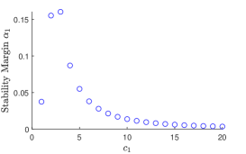
(a)

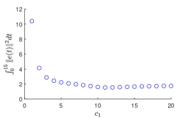
(b)

Figure 4. The closed-loop stability margin and $\int_{0}^{15}\lVert e(t)\rVert^{2}dt$ for the passive controller with $c_{2}=4$

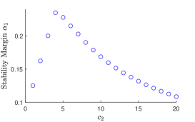
(a)

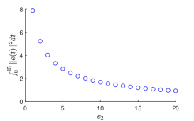
(b)

Figure 5. The closed-loop stability margin and $\int_{0}^{15}\lVert e(t)\rVert^{2}dt$ for the passive controller with $c_{1}=2.5$

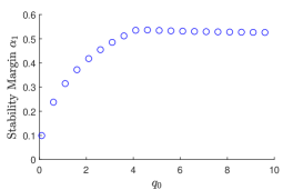
(a)

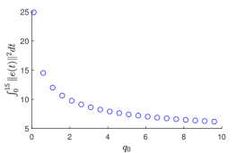
(b)

Figure 6. The closed-loop stability margin and $\int_{0}^{15}\lVert e(t)\rVert^{2}dt$ for the observer based controller with $R=0.1I_{2}$

(a)

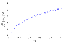
(b)

Figure 7. The closed-loop stability margin and $\int_{0}^{15}\lVert e(t)\rVert^{2}dt$ for the observer based controller with $Q=10I_{Z_{0}}$

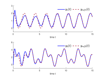
Figure 8. Output tracking using a passive controller

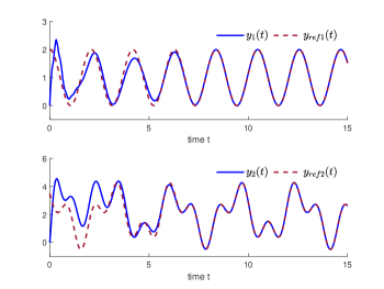
Figure 9. Output tracking using an observer based controller

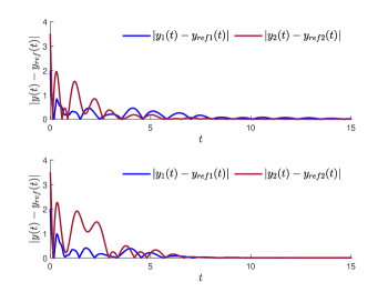
Figure 10. Tracking errors for passive(above) and observer based(below) controllers

The components of the observer based controller are chosen as in Section 4.1.2. The matrix $H$ is obtained by solving the system (51), where we use the approximations $A^{N}$ and $C^{N}$ in place of $A$ and $C$, respectively. The gain matrix $K_{1}$ is obtained using Matlab lqr function with $Q=q_{0}I_{Z_{0}},\ q_{0}>0$ and $R=r_{0}I_{2},r_{0}>0$. To maximize the stability margin, ranges of values of the parameters $q_{0}$ and $r_{0}$ were tested. The closed-loop stability margin $\alpha_{1}$ and $\int_{0}^{15}{\lVert e(t)\rVert^{2}dt}$ for different parameter values are plotted in Figures 6 and 7, respectively. It is observed that smaller control gains $r_{0}$ and larger $q_{0}$ result in larger closed-loop stability margin and smaller transient errors. By choosing $q_{0}=10$ and $r_{0}=0.1$, the output tracking and the tracking errors are depicted in Figures 9 and 10, respectively.

It can be seen from the figures that both controllers achieve tracking of the given reference signals asymptotically and the tracking error decays to zero at an exponential rate. Moreover, we can see that the observer based controller can achieve larger closed-loop stability margin and therefore the asymptotic error convergence for the observer based controller is faster than that for the passive controller. On the other hand, it is noted that even though the passive controller is a finite-dimensional controller and also the controller requires no information about the satellite system apart from passivity, it still achieves comparable performance to the infinite-dimensional observer based controller.

5. Conclusion

We investigated robust output tracking problem of a flexible satellite composed of two identical flexible solar panels and a center rigid body. A detailed proof of exponential stability of the model was presented. We constructed two robust controllers for the robust output tracking of the satellite model. Moreover, simulation results showing the performances of the controllers were presented.

References

• [1] S. Aoues, F. L. Cardoso-Ribeiro, D. Matignon, and D. Alazard. Modeling and control of a rotating flexible spacecraft: A port-Hamiltonian approach. IEEE Transactions on Control Systems Technology, 27(1):355–362, 2019.
• [2] K. Asti. Numerical approximation of dynamic Euler–Bernoulli beams and a flexible satellite. Master’s thesis. https://urn.fi/URN:NBN:fi:tuni-202008136475.
• [3] B. Augner. Uniform exponential stabilisation of serially connected inhomogeneous Euler-Bernoulli beams. ESAIM. Control, Optimisation and Calculus of Variations, 26:Paper No. 110, 24, 2020.
• [4] B. Augner. Well-posedness and stability for interconnection structures of port-Hamiltonian type. In Control theory of infinite-dimensional systems, volume 277 of Operator Theory:Advances and Applications, pages 1–52. Springer, 2020.
• [5] B. Augner and B. Jacob. Stability and stabilization of infinite-dimensional linear port-Hamiltonian systems. Evolution Equations and Control Theory, 3(2):207–229, 2014.
• [6] J. Bontsema, R. F. Curtain, and J. M. Schumacher. Robust control of flexible structures a case study. Automatica, 24(2):177–186, 1988.
• [7] G. Chen, S. A. Fulling, F. J. Narcowich, and S. Sun. Exponential decay of energy of evolution equations with locally distributed damping. SIAM Journal on Applied Mathematics, 51(1):266–301, 1991.
• [8] R. F. Curtain and H. J. Zwart. An introduction to infinite-dimensional linear systems theory, volume 21 of Texts in Applied Mathematics. Springer-Verlag, New York, 1995.
• [9] E. Davison. The robust control of a servomechanism problem for linear time-invariant multivariable systems. IEEE Transactions on Automatic Control, 21(1):25–34, 1976.
• [10] B. A. Francis and W. M. Wonham. The internal model principle for linear multivariable regulators. Applied Mathematics and Optimization, 2(2):170–194, 1975.
• [11] T. Govindaraj, J-P. Humaloja, and L. Paunonen. Robust output regulation of a flexible satellite. IFAC-PapersOnLine, 53(2):7795–7800, 2020.
• [12] T. Hämäläinen and S. Pohjolainen. Robust regulation of distributed parameter systems with infinite-dimensional exosystems. SIAM Journal on Control and Optimization, 48(8):4846–4873, 2010.
• [13] W. He and S. S. Ge. Dynamic modeling and vibration control of a flexible satellite. IEEE Transactions on Aerospace and Electronic Systems, 51(2):1422–1431, 2015.
• [14] B. Jacob and H. J. Zwart. Linear Port-Hamiltonian Systems on Infinite-Dimensional Spaces. Birkhäuser, 2011.
• [15] Y. Le Gorrec, H. Zwart, and B. Maschke. Dirac structures and boundary control systems associated with skew-symmetric differential operators. SIAM Journal on Control and Optimization, 44(5):1864–1892, 2005.
• [16] Z-H. Luo, B-Z. Guo, and O. Morgul. Stability and stabilization of infinite dimensional systems with applications. Communications and Control Engineering Series. Springer-Verlag, London, 1999.
• [17] L. Paunonen. Controller design for robust output regulation of regular linear systems. IEEE Transactions on Automatic Control, 61(10):2974–2986, 2016.
• [18] L. Paunonen. Stability and robust regulation of passive linear systems. SIAM Journal on Control and Optimization, 57(6):3827–3856, 2019.
• [19] L. Paunonen and S. Pohjolainen. The internal model principle for systems with unbounded control and observation. SIAM Journal on Control and Optimization, 52(6):3967–4000, 2014.
• [20] R. Rebarber and G. Weiss. Internal model based tracking and disturbance rejection for stable well-posed systems. Automatica, 39(9):1555–1569, 2003.
• [21] M. Tucsnak and G. Weiss. Observation and Control for Operator Semigroups. Birkhäuser, 2009.
• [22] X. Zhao and G. Weiss. Well-posedness, regularity and exact controllability of the SCOLE model. Mathematics of Control, Signals, and Systems, 22(2):91–127, 2010.
• [23] X. Zhao and G. Weiss. Strong stability of a coupled system composed of impedance-passive linear systems which may both have imaginary eigenvalues. In IEEE Conference on Decision and Control (CDC), pages 521–526, 2018.
• [24] Xiaowei Zhao and George Weiss. Controllability and observability of a well-posed system coupled with a finite-dimensional system. IEEE Transactions on Automatic Control, 56(1):88–99, 2011.
• [25] Xiaowei Zhao and George Weiss. Stability properties of coupled impedance passive LTI systems. IEEE Transactions on Automatic Control, 62(11):5769–5779, 2017.