Energy-stable global radial basis function methods on summation-by-parts form

Abstract

Radial basis function methods are powerful tools in numerical analysis and have demonstrated good properties in many different simulations. However, for time-dependent partial differential equations, only a few stability results are known. In particular, if boundary conditions are included, stability issues frequently occur. The question we address in this paper is how provable stability for RBF methods can be obtained. We develop and construct energy-stable radial basis function methods using the general framework of summation-by-parts operators often used in the Finite Difference and Finite Element communities.

65N35, 65N12, 65D12, 65D25

1 Introduction

We investigate energy stability of global radial basis function (RBF) methods for time-dependent partial differential equations (PDEs). Unlike finite differences (FD) or finite element (FE) methods, RBF schemes are mesh-free, making them flexible with respect to the geometry of the computational domain since the only used geometrical property is the pairwise distance between two centers. Further, they are suitable for problems with scattered data like in climate [10, 28] or stock market [5, 33] simulations. Finally, for smooth solutions, one can reach spectral convergence [9, 11]. In addition, they have recently become more and more popular for solving time-dependent problems in quantum mechanics, fluid dynamics, etc. [6, 24, 25, 40]. One distinguishes between global RBF methods (Kansa’s methods) [26] and local RBF methods, such as the RBF generated finite difference (RBF-FD) [39] and RBF partition of unity (RBF-PUM) [42] method. See the monograph [12] and references therein.
Even though their efficiency and good performance have been demonstrated for various problems, only a few stability results are known for advection-dominated problems. For example, an eigenvalue analysis was performed for a linear advection equation in [34], and it was found that RBF discretizations often produced eigenvalues lending to an exponential increase of the $L_{2}$ norm when boundary conditions were introduced. To illustrate this, consider the following example (also found in [18, Section 6.1]):

(1) $$\partial_{t}u+\partial_{x}u=0,\qquad u(x,0)=\mathrm{e}^{-20x^{2}}$$

with $x\in[-1,1]$, $t>0$, and where periodic boundary conditions are applied. In this example, a bump is traveling to the right, leaving the domain and coming back to the left.

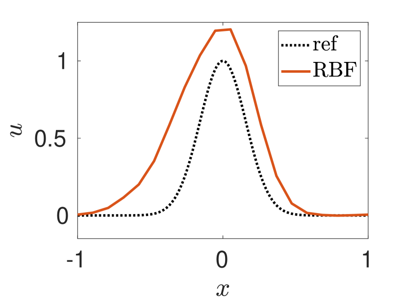
(a) Numerical solution at $t=10$

(b) Energy profile developing in time

Figure 1: Gaussian kernel with $N=20$ points (equidistant points) after 10 periods

In Figure 1, we plot the numerical solution and its energy up to $t=10$ using a global RBF method with a Gaussian kernel and $N=20$ points. An increase of the size of the bump and of the $L_{2}$ energy can be seen. For longer times, the computation breaks down. The discrete setting does not reflect the continuous one with zero energy growth and demonstrates the stability problems.
To overcome those, it was shown in [18, 19] that a weak formulation could result in a stable method. Recently, $L_{2}$ estimates were obtained using an oversampling technique [41]. Both these efforts use special techniques, and the question we address in this paper is how to stabilize RBF methods in a general way.
Classical summation-by-parts (SBP) operators were introduced during the 1970s in the context of FD schemes and they allow for a systematic development of energy-stable semi-discretizations of well-posed initial-boundary-value problems (IBVPs) [7, 38]. The SBP property is a discrete analog to integration by parts, and proofs from the continuous setting carry over directly to the discrete framework [31] if proper boundary procedures are added [38]. First based on polynomial approximations, the SBP theory has recently been extended to general function spaces developing so-called FSBP operators in [20]. Here, we investigate stability of global RBF methods through the lens of the FSBP theory.
We demonstrate that many existing RBF discretizations do not satisfy the FSBP property, which opens up for instabilities in these methods. Based on these findings, we show how RBF discretizations can be modified to obtain an SBP property. This then allows for a systematic development of energy-stable RBF methods. We give a couple of concrete examples including the most frequently used RBFs, where $L_{2}$ estimates are derived using an oversampling technique. For simplicity, we focus on the univariate setting for developing an SBP theory in the context of global RBF methods. That said, RBF methods and SBP operators can easily be extended to the multivariate setting, which is also demonstrated in our numerical tests.
The rest of this work is organized as follows. In Section 2, we provide some preliminaries on energy-stability of IBVPs and global RBF methods. Next, the concept of FSBP operators is shortly revisited in Section 3. We adapt the FSBP theory to RBF function spaces in Section 4. Here, it is also demonstrated that many existing RBF methods do not satisfy the SBP property and how to construct RBF operators in SBP form (RBFSBP). In Section 5, we give a couple of concrete examples of RBFSBP operators resulting in energy-stable methods. Finally, we provide numerical tests in Section 6 and concluding thoughts in Section 7.

2 Preliminaries

We now provide a few preliminaries on IBVPs and RBF methods.

2.1 Well-posedness and Energy Stability

Following [23, 31, 38], we consider

(2) $$\partial_{t}u =\mathcal{L}(x,t,\partial_{x})u+\mathcal{F},\quad x_{L}<x<x_{R},\ t>0,$$

$$u(x,0) =f(x),\quad x_{L}\leq x\leq x_{R},$$

$$\mathcal{B}_{0}(t,\partial_{x})u(x_{L},t) =g_{x_{L}}(t),\quad t\geq 0,$$

$$\mathcal{B}_{1}(t,\partial_{x})u(x_{R},t) =g_{x_{R}}(t),\quad t\geq 0,$$

where $u$ is the solution and $\mathcal{L}$ is a differential operator with smooth coefficients. Further, $B_{0}$ and $B_{1}$ are operators defining the boundary conditions, $\mathcal{F}$ is a forcing function, $f$ is the initial data, and $g_{x_{L}},g_{x_{R}}$ denote the boundary data. Examples of Eq. 2 include the advection equation

(3) $$\partial_{t}u(x,t)+a\partial_{x}u(x,t)=0$$

with constant $a\in\mathbb{R}$, the diffusion equation

(4) $$\partial_{t}u(x,t)=\partial_{x}\left(\kappa\partial_{x}u(x,t)\right)$$

with $\kappa\in\mathbb{R}$ depending on $x,t$, as well as combinations of Eqs. 3 and 4. Let us now formalize what we mean by the IBVP Eq. 2 being well-posed.

Definition 2.1.

The IBVP Eq. 2 with $\mathcal{F}=g_{x_{L}}=g_{x_{R}}=0$ is well-posed, if for every $f\in C^{\infty}$ that vanishes in a neighborhood of $x=x_{L},x_{R}$, Eq. 2 has a unique smooth solution $u$ that satisfies

(5) $$\mathinner{\!\left\lVert u(\cdot,t)\right\rVert}_{L_{2}}\leq C\mathrm{e}^{\alpha_{C}t}\mathinner{\!\left\lVert f\right\rVert}_{L_{2}},$$

where $C,\alpha_{c}$ are constants independent of $f$. Moreover, the IBVP Eq. 2 is strongly well-posed, if it is well-posed and

(6) $$\mathinner{\!\left\lVert u(\cdot,t)\right\rVert}^{2}_{L_{2}}\leq C(t)\left(\mathinner{\!\left\lVert f\right\rVert}^{2}_{L_{2}}+\int_{0}^{t}\left(\mathinner{\!\left\lVert\mathcal{F}(\cdot,\tau)\right\rVert}^{2}_{L_{2}}+|g_{x_{L}}(\tau)|^{2}+|g_{x_{R}}(\tau)|^{2}\right)d\tau\right),$$

holds, where the function $C(t)$ is bounded for finite $t$ and independent of $\mathcal{F},g_{x_{L}},g_{x_{R}}$, and $f$.

Switching to the discrete framework, our numerical approximation $u^{h}$ of Eq. 2 should be constructed in such a way that similar estimates to Eq. 5 and Eq. 6 are obtained. We denote our grid quantity (a measure of the grid size) by $h$. In the context of RBF methods, $h$ denotes the maximum distance between two neighboring points. We henceforth denote by $\|\cdot\|_{h}$ a discrete version of the $L_{2}$-norm and $\mathinner{\!\left\lVert\cdot\right\rVert}_{b}$ represents a discrete boundary norm. Then, we define stability of the numerical solution as follows.

Definition 2.2.

Let $\mathcal{F}=g_{x_{L}}=g_{x_{R}}=0$ and $f^{h}$ be an adequate projection of the initial data $f$ which vanishes at the boundaries. The approximation $u^{h}$ is stable if

(7) $$\mathinner{\!\left\lVert u^{h}(t)\right\rVert}^{2}_{h}\leq C\mathrm{e}^{\alpha_{d}t}\mathinner{\!\left\lVert f^{h}\right\rVert}_{h}$$

holds for all sufficiently small $h$, where $C$ and $\alpha_{d}$ are constants independent of $f^{h}$. The approximated solution $u^{h}$ is called strongly energy stable if it is stable and

(8) $$\mathinner{\!\left\lVert u^{h}(t)\right\rVert}^{2}_{h}\leq C(t)\left(\mathinner{\!\left\lVert f^{h}\right\rVert}^{2}_{h}+\max\limits_{\tau\in[0,t]}\mathinner{\!\left\lVert\mathcal{F}(\tau)\right\rVert}_{h}^{2}+\max\limits_{\tau\in[0,t]}\mathinner{\!\left\lVert g_{x_{L}}(\tau)\right\rVert}^{2}_{b}+\max\limits_{\tau\in[0,t]}\mathinner{\!\left\lVert g_{x_{R}}(\tau)\right\rVert}^{2}_{b}\right)$$

holds for all sufficiently small $h$. The function $C(t)$ is bounded for finite $t$ and independent of $\mathcal{F},g_{x_{L}},g_{x_{R}}$, and $f^{h}$.

2.2 Discretization

To discretize the IBVP Eq. 2, we apply the method of lines. The space discretization is done using a global RBF method resulting in a system of ordinary differential equations (ODEs):

(9) $$\frac{\mathrm{d}}{\mathrm{d}t}\mathbf{u}=\operatorname{L}(\mathbf{u}).$$

Here, $\mathbf{u}$ denotes the vector of coefficients and $\operatorname{L}$ represents the spatial operator. We used the explicit strong stability preserving (SSP) Runge–Kutta (RK) method of third-order with three stages (SSPRK(3,3)) [36] for all subsequent numerical tests.

2.2.1 Radial Basis Function Interpolation

RBFs are powerful tools for interpolation and approximation [43, 8, 12]. In the context of the present work, we are especially interested in RBF interpolants. Let $u\mathrel{\mathop{\ordinarycolon}}\mathbb{R}\supset\Omega\to\mathbb{R}$ be a scalar valued function and $X_{K}=\{x_{1},\dots,x_{K}\}$ a set of interpolation points, referred to as centers. The RBF interpolant of $u$ is

(10) $$u^{h}(x)=\sum_{k=1}^{K}\alpha_{k}\varphi(|x-x_{k}|)+\sum_{l=1}^{m}\beta_{k}p_{l}(x).$$

Here, $\varphi\mathrel{\mathop{\ordinarycolon}}\mathbb{R}_{0}^{+}\to\mathbb{R}$ is the RBF (also called kernel) and $\{p_{l}\}_{l=1}^{m}$ is a basis for the space of polynomials up to degree $m-1$, denoted by $\mathbb{P}_{m-1}$. Furthermore, the RBF interpolant Eq. 10 is uniquely determined by the conditions

(11) $$u^{h}(x_{k}) =u(x_{k}),\quad k=1,\dots,K,$$

(12) $$\sum_{k=1}^{K}\alpha_{k}p_{l}(x_{k}) =0,\quad l=1,\dots,m.$$

Note that Eq. 11 and Eq. 12 can be reformulated as a linear system for the coefficient vectors $\boldsymbol{\alpha}=[\alpha_{1},\dots,\alpha_{K}]^{T}$ and $\boldsymbol{\beta}=[\beta_{1},\dots,\beta_{m}]^{T}$:

(13) $$\begin{bmatrix}\Phi&\mathrm{P}\\ \mathrm{P}^{T}&0\end{bmatrix}\begin{bmatrix}\boldsymbol{\alpha}\\ \boldsymbol{\beta}\end{bmatrix}=\begin{bmatrix}\mathbf{u}\\ \mathbf{0}\end{bmatrix},$$

where $\mathbf{u}=[u(x_{1}),\dots,u(x_{K})]^{T}$ and

(14) $$\Phi=\begin{bmatrix}\varphi(|x_{1}-x_{1}|)&\dots&\varphi(|x_{1}-x_{K}|)\\ \vdots&&\vdots\\ \varphi(|x_{K}-x_{1}|)&\dots&\varphi(|x_{K}-x_{K}|)\end{bmatrix},\ \mathrm{P}=\begin{bmatrix}p_{1}(x_{1})&\dots&p_{m}(x_{1})\\ \vdots&&\vdots\\ p_{1}(x_{K})&\dots&p_{m}(x_{K})\end{bmatrix}.$$

Incorporating polynomial terms of degree up to $m-1$ in the RBF interpolant Eq. 10 is important for several reasons:

1. The RBF interpolant Eq. 10 becomes exact for polynomials of degree up to $m-1$, i. e., $u^{h}=u$ for $u\in\mathbb{P}_{m-1}$.

2. For some (conditionally positive) kernels $\varphi$, the RBF interpolant Eq. 10 only exists uniquely when polynomials up to a certain degree are incorporated.

In addition, we will show that (i) is needed for the RBF method to be conservative [18, 20]. The property (ii) is explained in more detail in Appendix A as well as in [8, Chapter 7] and [15, Chapter 3.1]. For simplicity and clarity, we will focus on the choices of RBFs listed in Table 1. More types of RBFs and their properties can be found in the monographs [43, 8, 12].

RBF	$\varphi(r)$	parameter	order
Gaussian	$\exp(-(\varepsilon r)^{2})$	$\varepsilon>0$	0
Multiquadrics	$\sqrt{1+(\varepsilon r)^{2}}$	$\varepsilon>0$	$1$
Polyharmonic splines (odd)	$r^{2k-1}$	$k\in\mathbb{N}$	$k$
Polyharmonic splines (even)	$r^{2k}\log r$	$k\in\mathbb{N}$	$k+1$

Table 1: Some frequently used RBFs

Note that the set of all RBF interpolants Eq. 10 forms a $K$-dimensional linear space, denoted by $\mathcal{R}_{m}(X_{K})$. This space is spanned by the cardinal functions

(15) $$c_{i}(x)=\sum_{k=1}^{K}\alpha_{k}^{(i)}\varphi(|x-x_{k}|)+\sum_{l=1}^{m}\beta^{(i)}_{l}p_{l}(x),\quad i=1,\dots,K,$$

which are uniquely determined by the cardinal property

(16) $$c_{i}(x_{k})=\delta_{ik}\mathrel{\mathop{\ordinarycolon}}=\begin{cases}1&\text{if }i=k,\\ 0&\text{otherwise},\end{cases}\quad i,k=1,\dots,K,$$

and condition Eq. 12. They also provide us with the following (nodal) representation of the RBF interpolant:

(17) $$u^{h}(x)=\sum_{k=1}^{K}u(x_{k})c_{k}(x).$$

2.2.2 Radial Basis Function Methods

We outline the standard global RBF method for the IBVP Eq. 2. The domain $\Omega$ on which we solve (2) is discretized using two point sets:

• The nodal point set (centers) $X_{K}=\{x_{1},\cdots,x_{K}\}$ used for constructing the cardinal basis functions Eq. 15.

• The grid (evaluation) point set $Y_{N}=\{y_{1},\cdots,y_{N}\}$ for describing the IBVP (2), where $N\geq K$.

By selecting $Y_{N}=X_{K}$, we get a collocation method, and with $N>K$, a method using oversampling. The numerical solution $\mathbf{u}$ is defined by the values of $u^{h}$ at $Y_{N}$ and the operator $L(\mathbf{u})$ by using the spatial derivative of the RBF interpolant $u^{h}$, also at $Y_{N}$. The RBF discretization can be summarized in the following three steps:

1. Determine the RBF interpolant $u^{h}\in\mathcal{R}_{m}(X_{K})$.

2. Define $L(\mathbf{u})$ in the semidiscrete equation by inserting Eq. 17 into the continuous spatial operator. This yields

   (18) $$\operatorname{L}(\mathbf{u})= \left(\mathcal{L}(y_{n},t,\partial_{x})u^{h}(t,y_{n})+\mathcal{F}(t,y_{n})\right)_{n=1}^{N}.$$

3. Use a classical time integration scheme to evolve Eq. 9.

Global RBF methods come with several free parameters. These include the center and evaluation points $X_{K}$ and $Y_{N}$, the kernel $\varphi$, the degree $m-1$ of the polynomial term included in the RBF interpolant Eq. 10. The kernel $\varphi$ might come with additional free parameters such as the shape parameter $\varepsilon$. Finally, we note that also the basis of the RBF approximation space $\mathcal{R}_{m}(X_{K})$, that one uses for numerically computing the RBF approximation $u^{h}$ and its derivatives, can influence how well-conditioned the RBF method is in practice. Discussions of appropriate choices for these parameters are filling whole books [43, 8, 13, 12] and are avoided here. In this work, we have a different point in mind and focus on the basic stability conditions of RBF methods.

3 Summation-by-parts Operators on General Function Spaces

SBP operators were developed to mimic the behavior of integration by parts in the continuous setting and provide a systematic way to build energy-stable semi-discrete approximations. First, constructed for an underlying polynomial approximation in space, the theory was recently extended to general function spaces in [20]. For completeness, we shortly review the extended framework of FSBP operators and repeat their basic properties. We consider the FSBP concept on the interval $[x_{L},x_{R}]$ where the boundary points are included in the evaluation points $Y_{N}$. Using this framework, we give the following definition originally found in [20]:

Definition 3.1 (FSBP operators).

Let $\mathcal{F}\subset C^{1}([x_{L},x_{R}])$ be a finite-dimensional function space. An operator $D=P^{-1}Q$ is an $\mathcal{F}$-based SBP (FSBP) operator if

1. $Df(\mathbf{x})=f^{\prime}(\mathbf{x})$ for all $f\in\mathcal{F}$,

2. $P$ is a symmetric positive definite matrix, and

3. $Q+Q^{T}=B=\operatorname{diag}(-1,0,\dots,0,1)$.

Here, $f(\mathbf{y})=[f(y_{1}),\dots,f(y_{N})]^{T}$ and $f^{\prime}(\mathbf{y})=[f^{\prime}(y_{1}),\dots,f^{\prime}(y_{N})]^{T}$ respectively denote the vector of the function values of $f$ and its derivative $f^{\prime}$ at the evaluation points $y_{1},\dots,y_{N}$.
Further, $D$ denotes the differentiation matrix and $P$ is a matrix defining a discrete norm. In order to produce an energy estimate, $P$ must be positive definite and symmetric. In this manuscript and in [20], we focus for stability reasons on diagonal norm FSBP operators [29, 14, 35]. The matrix $Q$ is nearly skew-symmetric and can be seen as the stiffness matrix in context of FE. With these operators, integration-by-parts is mimicked discretely as:

(19) $$f(\mathbf{x})^{T}PDg(\mathbf{x})+\left(Df(\mathbf{x})\right)^{T}Pg(\mathbf{x}) =f(\mathbf{x})^{T}Bg(\mathbf{x})$$

$$\Longleftrightarrow \int_{x_{L}}^{x_{R}}f(x)\cdot g^{\prime}(x)dx+\int_{x_{L}}^{x_{R}}f^{\prime}(x)\cdot g(x)dx =[f(x)g(x)]_{x=x_{L}}^{x=x_{R}}$$

for all $f,g\in\mathcal{F}$.

3.1 Properties of FSBP Operators

In [20], the authors proved that the FSBP-SAT semi-discretization of the linear advection equation yields an energy stable semi-discretization. The so-called SAT term imposes the boundary condition weakly. Moreover, the underyling function space $\mathcal{F}$ should contain constants in order to ensure conservations.

In context of RBF methods, constants have to be included in the RBF interpolants Eq. 10, also for the reasons discussed above.
We will extend the previous investigation to the linear advection-diffusion equation.

(20) $$\partial_{t}u+a\partial_{x}u =\partial_{x}(\kappa\partial_{x}u),\quad x\in(x_{L},x_{R}),\ t>0,$$

$$u(x,0) =f(x),$$

$$au(x_{L},t)-\kappa\partial_{x}u(x_{L},t) =g_{x_{L}}(t),$$

$$\kappa\partial_{x}u(x_{R},t) =g_{x_{R}}(t),$$

where $a>ß$ is a constant and $\kappa>0$ can depend on $x$ and $t$. The problem (20) is strongly well-posed, as can be seen by the energy rate

(21) $$\mathinner{\!\left\lVert u\right\rVert}_{t}^{2}+2\mathinner{\!\left\lVert u_{x}\right\rVert}^{2}_{\kappa}= a^{-1}\bigg{(}g_{x_{L}}^{2}-\left(au(x_{L},t)-g_{x_{L}}\right)^{2}-\left(au(x_{R},t)-g_{x_{R}}^{2}\right)^{2}+g_{x_{R}}^{2}\bigg{)}$$

with $\mathinner{\!\left\lVert u_{x}\right\rVert}^{2}_{\kappa}=\int_{x_{L}}^{x_{R}}(\partial_{x}u)^{2}\kappa\mathrm{d}x.$ To translate this estimate to the discrete setting, we discretize (20). The most straightforward FSBP-SAT discretization reads

(22) $$\mathbf{u}_{t}+aD\mathbf{u}=D(\mathcal{K}D\mathbf{u})+P^{-1}\mathbb{S}$$

with $\mathcal{K}=\operatorname{diag}(\kappa)$ and

(23) $$\mathbb{S}\mathrel{\mathop{\ordinarycolon}}=[\mathbb{S}_{0},0,\dots,\mathbb{S}_{1}]^{T},\\ \mathbb{S}_{0}\mathrel{\mathop{\ordinarycolon}}=-\sigma_{0}a(u_{0}-(\mathcal{K}D\mathbf{u})_{0}-g_{x_{L}}),\\ \mathbb{S}_{1}\mathrel{\mathop{\ordinarycolon}}=-\sigma_{1}((\mathcal{K}D\mathbf{u})_{N}-g_{x_{R}}).$$

We can prove the following result using the FSBP Definition 3.1.

Theorem 3.2.

The scheme (22) is strongly stable with $\sigma_{0}=-1$ and $\sigma_{1}=1$.

Proof 3.3.

We use the energy method together with the FSBP property to obtain

(24) $$\mathinner{\!\left\lVert\mathbf{u}\right\rVert}_{t}^{2}+2\mathinner{\!\left\lVert D\mathbf{u}\right\rVert}^{2}_{\mathcal{K}}=a^{-1}\left(g_{x_{L}}^{2}-(au_{0}-g_{x_{L}})^{2}-(au_{N}-g_{x_{R}})^{2}+g_{x_{R}}^{2}\right)$$

with $\mathinner{\!\left\lVert D\mathbf{u}\right\rVert}^{2}_{\mathcal{K}}=(D\mathbf{u})^{T}P\mathcal{K}D\mathbf{u}$. This is similar to the continuous estimate (21). Note that $P$ and $\mathcal{K}$ have to be diagonal to ensure that $P\mathcal{K}$ defines a norm.

Clearly, the FSBP operators automatically reproduce the results from the continuous setting, similar to the classical SBP operators based on polynomial approximations [38]. Note that no details are assumed on the specific function space, grid or the underlying methods. The only factors of importance is that the FSBP property is fulfilled and that well posed boundary condition are used. In what follows, we will adapt the FSBP theory to radial basis functions.

4 SBP operators for RBFs

First, we adapt the FSBP theory in Section 2.2 to the RBF framework. Next, we investigate classical RBF methods concerning the FSBP property, and demonstrate that standard global RBF schemes does not fulfill this property. Finally, we describe how RBFSBP operators can be constructed that lead to stability.

4.1 RBF-based SBP operators

The function space $\mathcal{F}\subset C^{1}$ for RBF methods is defined by the description in Subsection 2.2. Consider a set of $K$ points, $X_{K}=\{x_{1},\cdots,x_{K}\}\subset[x_{L},x_{R}]$. The set of all RBF interpolants Eq. 10 forms a $K$-dimensional approximation space, which we denote by $\mathcal{R}_{m}(X_{K})$. Let $\{c_{k}\}_{k=1}^{K}$ be a basis in $\mathcal{R}_{m}(X_{K})$. Further, we have the grid points $Y_{N}=\{y_{1},\cdots,y_{N}\}\subset[x_{L},x_{R}]$ which include the boundaries. They are used to define the RBFSBP operators.

Definition 4.1 (RBF Summation-by-Parts Operators).

An operator $D=P^{-1}Q\in\mathbb{R}^{N\times N}$ is an RBFSBP operator on the grid points $Y_{N}$ if

1. $Dc_{k}(\mathbf{x})=c_{k}^{\prime}(\mathbf{x})$ for $k=1,2,\dots,K$ and $c_{k}\in\mathcal{R}_{m}(X_{K})$,

2. $P\in\mathbb{R}^{N\times N}$ is a symmetric positive definite matrix, and

3. $Q+Q^{T}=B$.

In the classical RBF discretizations, the exactness of the derivatives of the cardinal functions is the only condition which is imposed. However, to construct energy stable RBF methods, the existence of an adequate norm is as important as the condition on the derivative matrix. Hence it is often necessary to use a higher number of grid points than centers to ensure the existence of a positive quadrature formula to guarantee the conditions in Definition 4.1.
The norm matrix $P$ in Definition 4.1 has only been assumed to be symmetric positive definite. However, as mentioned above for the remainder of this work, we restrict ourselves to diagonal norm matrices $P=\operatorname{diag}(\omega_{1},\cdots,\omega_{N})$ where $\omega_{i}$ is the associated quadrature weight because Diagonal-norm operators are

1. required for certain splitting techniques [14, 30, 32], and variable coefficients, see for example (24).

2. better suited to conserve nonquadratic quantities for nonlinear stability [27],

3. easier to extend to, for instance, curvilinear coordinates [4, 35, 37].

Remark 4.2.

In Definition 4.1, we have two sets of points, the interpolation points $X_{K}$ and the grid points $Y_{N}$. The derivative matrix is constructed with respect to the exactness of the cardinal functions $c_{k}$ related to the interpolation points $X_{K}$. However, all operators are constructed with respect to the grid points $Y_{N}$, i.e. $D,P,Q\in\mathbb{R}^{N\times N}$. This is in particular essential when ensuring the existence of suitable norm matrix $P$. This means that the size of the SBP operator is determine by the quadrature formula. So, the number of grid points and their placing highly effects the size of the operators and so the efficiency of the underlying method itself. In the future, this will be investigated in more detail.

4.2 Existing Collocation RBF Methods and the FSBP Property

In the classical collocation RBF approach, the centers intersect with the grid points, i.e. $X_{K}=Y_{N}$. It was shown in [20] that a diagonal-norm $\mathcal{F}$-exact SBP operator exists on the grid $Y_{N}=\{y_{1},\cdots,y_{N}\}$ if and only if a positive and $(\mathcal{F}\mathcal{F})^{\prime}$-exact quadrature formula exists on the same grid (the same requirement as for classical SBP operators). The differentiation matrix $D\in\mathbb{R}^{N\times N}$ of a collocation RBF method can thus only satisfy the FSBP property if there exists a positive and $(\mathcal{R}_{m}(Y_{N})\mathcal{R}_{m}(Y_{N}))^{\prime}$-exact quadrature formula on the grid $Y_{N}$. The weights $\mathbf{w}\in\mathbb{R}^{N}$ of such a quadrature formula would have to satisfy

(25) $$G\mathbf{w}=\mathbf{m},\quad\mathbf{w}>0,$$

with the coefficient matrix $G$ and vector of moments $\mathbf{m}$ given by

(26) $$G=\begin{bmatrix}g_{1}(y_{1})&\dots&g_{1}(y_{N})\\ \vdots&&\vdots\\ g_{L}(y_{1})&\dots&g_{L}(y_{N})\end{bmatrix},\quad\mathbf{m}=\begin{bmatrix}\int_{a}^{b}g_{1}(y)\,\mathrm{d}y\\ \vdots\\ \int_{a}^{b}g_{L}(y)\,\mathrm{d}y\end{bmatrix},$$

In (26), $\{g_{l}\}_{l=1}^{L}$ is a basis of the function space $(\mathcal{R}_{m}(Y_{N})\mathcal{R}_{m}(Y_{N}))^{\prime}$. In many cases, the dimension $L$ of $(\mathcal{R}_{m}(Y_{N})\mathcal{R}_{m}(Y_{N}))^{\prime}$ is larger than the dimension $N$ of $\mathcal{R}_{m}(Y_{N})$. In this case, $L>N$ and the linear system in Eq. 25 is overdetermined and has no solution. This is demonstrated in Table 2, which reports on the residual and smallest element of the least squares solution (solution with minimal $\ell^{2}$-error) of Eq. 25 for different cases. In all of our considered tests, the residuals were always larger than zero indicating that the operator is not in SBP form. Similar results are obtained for non-diagonal norm matrices $P$, which is outlined in Appendix B.

Equidistant points
		$\|G\mathbf{w}-\mathbf{m}\|_{2}$				$\min\mathbf{w}$
$N$/$m-1$		$0$	$1$	$2$		$0$	$1$	$2$
$10$		$7.6\cdot 10^{-1}$	$6.6\cdot 10^{-1}$	$1.3\cdot 10^{-12}$		$2.7\cdot 10^{-2}$	$3.3\cdot 10^{-2}$	$5.6\cdot 10^{-2}$
$20$		$6.9\cdot 10^{-1}$	$6.4\cdot 10^{-1}$	$6.1\cdot 10^{-11}$		$1.5\cdot 10^{-2}$	$1.6\cdot 10^{-2}$	$2.6\cdot 10^{-2}$
$40$		$6.6\cdot 10^{-1}$	$6.4\cdot 10^{-1}$	$2.5\cdot 10^{-9}$		$7.7\cdot 10^{-3}$	$8.0\cdot 10^{-3}$	$1.3\cdot 10^{-2}$

Halton points
		$\|G\mathbf{w}-\mathbf{m}\|_{2}$				$\min\mathbf{w}$
$N$/$m-1$		$0$	$1$	$2$		$0$	$1$	$2$
$10$		$1.0$	$1.0$	$5.6$		$3.1\cdot 10^{-4}$	$3.9\cdot 10^{-4}$	$5.6\cdot 10^{-3}$
$20$		$1.0$	$1.0$	$1.0\cdot 10^{1}$		$2.5\cdot 10^{-6}$	$2.7\cdot 10^{-6}$	$-4.3\cdot 10^{-3}$
$40$		$1.0$	$1.0$	$1.6\cdot 10^{1}$		$2.2\cdot 10^{-10}$	$2.3\cdot 10^{-10}$	$-1.3\cdot 10^{-3}$

Random points
		$\|G\mathbf{w}-\mathbf{m}\|_{2}$				$\min\mathbf{w}$
$N$/$m-1$		$0$	$1$	$2$		$0$	$1$	$2$
$10$		$1.3$	$1.2$	$1.5\cdot 10^{1}$		$1.1\cdot 10^{-6}$	$1.3\cdot 10^{-6}$	$-9.6\cdot 10^{-2}$
$20$		$1.1$	$1.1$	$1.1\cdot 10^{2}$		$5.6\cdot 10^{-16}$	$1.8\cdot 10^{-15}$	$-1.7\cdot 10^{-1}$
$40$		$1.3$	$1.3$	$1.8\cdot 10^{3}$		$-4.1\cdot 10^{-11}$	$-2.9\cdot 10^{-11}$	$-1.2\cdot 10^{1}$

Table 2: Residual $\|G\mathbf{w}-\mathbf{m}\|_{2}$ and smallest elements $\min\mathbf{w}$ for the cubic PHS-RBF on equidistant, Halton, and random points.

4.3 Existence and Construction of RBFSBP Operators

Translating the main result from [20], we need quadrature formulas to ensure the exact integration of $(\mathcal{R}_{m}(X_{K})\mathcal{R}_{m}(X_{K}))^{\prime}$. For RBF spaces, we use least-squares formulas, which can be used on almost arbitrary sets of grid points $Y_{N}$ and to any degree of exactness. The least squares ansatz always leads to a positive and $(\mathcal{R}_{m}(X_{K})\mathcal{R}_{m}(X_{K}))^{\prime}$-exact quadrature formula as long a sufficiently large number of data points $Y_{N}$ is used.

Remark 4.3.

Existing results on positivity and exactness of least squares quadrature formulas usually assume that the function space contains constants [16, 17]. Translating this to our setting, we need this property to be fulfilled for $(\mathcal{R}_{m}(X_{K})\mathcal{R}_{m}(X_{K}))^{\prime}$. Therefore, $\mathcal{R}_{m}(X_{K})$ should contain constants and linear functions. However, this assumption is primarily made for technical reasons and can be relaxed. Indeed, even when $\mathcal{R}_{m}(X_{K})$ only contained constants, we were still able to construct positive and $(\mathcal{R}_{m}(X_{K})\mathcal{R}_{m}(X_{K}))^{\prime}$-exact least squares quadrature formulas in all our examples. Future work will provide a theoretical justification for this.

Due to the least-square ansatz, we may always assume that we have a positive and
$(\mathcal{R}_{m}(X_{K})\mathcal{R}_{m}(X_{K}))^{\prime}$-exact quadrature formula. With that ensured, we summarize the algorithm to construct a diagonal norm RBFSBP operators in the following steps:

1. Build $P$ by setting the quadrature weights on the diagonal.

2. Split $Q$ into its known symmetric $\frac{1}{2}B$ and unknown anti-symmetric part $Q_{A}$.

3. Calculate $Q_{A}$ by using

   $$Q_{A}C=PC_{x}-\frac{1}{2}BC\text{ with }C=[c_{1}(\mathbf{y}),\dots,c_{K}(\mathbf{y})]=\begin{bmatrix}c_{1}(y_{1})&\dots&c_{K}(y_{1})\\ \vdots&&\vdots\\ c_{1}(y_{N})&\dots&c_{K}(y_{N})\end{bmatrix}$$

   and $C_{x}=[c_{1}^{\prime}(\mathbf{y}),\dots,c_{K}^{\prime}(\mathbf{y})]$ is defined analogous to $C$ where $\{c_{1},...,c_{K}\}$ is a basis of the K-dimensional function space.

4. Use $Q_{A}$ in $Q=Q_{A}+\frac{1}{2}B$ to calculate $Q$.

5. $D=P^{-1}Q$ gives the RBFSBP operator.

In the RBF context, one can always use cardinal functions as the basis. However, for simplicity reason is can be wise to use another basis representation, derived from the cardinal functions.

5 RBFSBP Operators

Next, we construct RBFSBP operators for a few frequently used kernels. We consider a set of $K$ points, ${X_{K}=\{x_{1},\dots,x_{K}\}\subset[x_{L},x_{R}]}$, and assume that these include the boundaries $x_{L}$ and $x_{R}$. Henceforth, we will consider the kernels listed in Table 1 and augment them with constants. The set of all RBF interpolants including constants Eq. 10 forms a $K$-dimensional approximation space, which we denote by $\mathcal{R}_{1}(X_{K})$. This space is spanned by the cardinal functions $c_{k}\in\mathcal{R}_{1}(X_{K})$ which are uniquely determined by (16). The matching constraint is then simply $\sum_{k=1}^{K}\alpha_{k}=0.$ That is,

(27) $$\mathcal{R}_{1}(X_{K})=\mathrm{span}\{\,c_{k}\mid k=1,\dots,K\,\}$$

with the approximation space $\mathcal{R}_{1}(X_{K})$ having dimension $K$.
The product space $\mathcal{R}_{1}(X_{K})\mathcal{R}_{1}(X_{K})$ and its derivative space $(\mathcal{R}_{1}(X_{K})\mathcal{R}_{m}(X_{K}))^{\prime}$ are respectively given by

(28) $$\mathcal{R}_{1}(X_{K})\mathcal{R}_{1}(X_{K}) =\mathrm{span}\{\,c_{k}c_{l}\mid k,l=1,\dots,K\,\},$$

(29) $$(\mathcal{R}_{1}(X_{K})\mathcal{R}_{1}(X_{K}))^{\prime} =\mathrm{span}\{\,c_{k}^{\prime}c_{l}+c_{k}c_{l}^{\prime}\mid k,l=1,\dots,K\,\}.$$

Note that the right-hand sides of Eq. 28 and Eq. 29 both use $K^{2}$ elements to span the product space $\mathcal{R}_{1}(X_{K})\mathcal{R}_{1}(X_{K})$ and its derivative space $(\mathcal{R}_{1}(X_{K})\mathcal{R}_{1}(X_{K}))^{\prime}$. However, these elements are not linearly independent and the dimensions of $\mathcal{R}_{1}(X_{K})\mathcal{R}_{1}(X_{K})$ and $(\mathcal{R}_{1}(X_{K})\mathcal{R}_{1}(X_{K}))^{\prime}$ are smaller than $K^{2}$. Indeed, we can observe that $c_{k}c_{l}=c_{l}c_{k}$ and the dimension of Eq. 28 is therefore bounded from above by

(30) $$\mathrm{dim}\,\mathcal{R}_{1}(X_{K})\mathcal{R}_{1}(X_{K})\leq\frac{K(K+1)}{2}.$$

Finally, we point out that in the calculation of the operators $P,Q$ and $D$ below, we will round the numbers to the second decimal place.

5.1 RBFSBP Operators using Polyharmonic Splines

In the first test, we work with cubic polyharmonic splines, $\varphi(r)=r^{3}$. On $[x_{L},x_{R}]=[0,1]$ and for the centers $X_{3}=\{0,1/2,1\}$, the three-dimensional cubic RBF approximation space Eq. 27 is given by $\mathcal{R}_{1}(X_{3})=\mathrm{span}\{\,c_{1},c_{2},c_{3}\,\}=\mathrm{span}\{\,b_{1},b_{2},b_{3}\,\}$ with cardinal functions

(31) $$c_{1}(x) =\frac{1}{2}|x|^{3}-2|x-1/2|^{3}+\frac{3}{2}|x-1|^{3}-\frac{1}{4},$$

$$c_{2}(x) =-2|x|^{3}+4|x-1/2|^{3}-2|x-1|^{3}+\frac{3}{2},$$

$$c_{3}(x) =\frac{3}{2}|x|^{3}-2|x-1/2|^{3}+\frac{1}{2}|x-1|^{3}-\frac{1}{4}$$

and alternative basis functions

$$b_{1}(x)=1,\quad b_{2}(x)=x^{3}-|x-1/2|^{3},\quad b_{3}(x)=x^{3}+(x-1)^{3}.$$

We make the transformation to the basis representation $\mathrm{span}\{b_{1},b_{2},b_{3}\}$ to simplify the determination of $(\mathcal{R}_{1}(X_{3})\mathcal{R}_{1}(X_{3}))^{\prime}$. In this alternative basis representation, the product space $\mathcal{R}_{1}(X_{3})\mathcal{R}_{1}(X_{3})$ and its derivative space $(\mathcal{R}_{1}(X_{3})\mathcal{R}_{1}(X_{3}))^{\prime}$ are respectively given by

(32) $$\mathcal{R}_{1}(X_{3})\mathcal{R}_{1}(X_{3}) =\mathrm{span}\{\,1,b_{2},b_{3},b_{2}^{2},b_{3}^{2},b_{2}b_{3}\,\}$$

$$(\mathcal{R}_{1}(X_{3})\mathcal{R}_{1}(X_{3}))^{\prime} =\mathrm{span}\{\,b_{2}^{\prime},b_{3}^{\prime},b_{2}^{\prime}b_{2},b_{3}^{\prime}b_{3},b_{2}^{\prime}b_{3}+b_{2}b_{3}^{\prime}\,\}.$$

Next, we have to find an $(\mathcal{R}_{1}(X_{3})\mathcal{R}_{1}(X_{3}))^{\prime}$-exact quadrature formula with positive weights. For the chosen $N=4$ equidistant grid points, the least-squares quadrature formula has positive weights and is $(\mathcal{R}_{1}(X_{3})\mathcal{R}_{1}(X_{3}))^{\prime}$-exact. The points and weights are $\mathbf{x}=\left[0,\frac{1}{3},\frac{2}{3},1\right]^{T}$ and $P=\operatorname{diag}\left(\frac{16}{129},\frac{81}{215},\frac{81}{215},\frac{16}{129}\right)$. The corresponding matrices $Q$ and $D$ of the RBFSBP operator $D=P^{-1}Q$ obtained from the construction procedure described before are

(33) $$Q\approx\left(\begin{array}[]{cccc}-\frac{1}{2}&\frac{59}{100}&-\frac{3}{20}&\frac{3}{50}\\ -\frac{59}{100}&0&\frac{37}{50}&-\frac{3}{20}\\ \frac{3}{20}&-\frac{37}{50}&0&\frac{59}{100}\\ -\frac{3}{50}&\frac{3}{20}&-\frac{59}{100}&\frac{1}{2}\end{array}\right),\quad D\approx\left(\begin{array}[]{cccc}-\frac{403}{100}&\frac{473}{100}&-\frac{121}{100}&\frac{51}{100}\\ -\frac{39}{25}&0&\frac{49}{25}&-\frac{2}{5}\\ \frac{2}{5}&-\frac{49}{25}&0&\frac{39}{25}\\ -\frac{51}{100}&\frac{121}{100}&-\frac{473}{100}&\frac{403}{100}\end{array}\right).$$

This example was presented with less details in [20].

5.2 RBFSBP Operators using Gaussian Kernels

Next, we consider the Gaussian kernel $\varphi(r)=\exp(-r^{2})$ on $[x_{L},x_{R}]=[0,1]$ for the centers $X_{3}=\{0,1/2,1\}$. The three-dimensional Gaussian RBF approximation space Eq. 27 is given by $\mathcal{R}_{1}(X_{3})=\mathrm{span}\{\,c_{1},c_{2},c_{3}\,\}$ with cardinal functions

(34) $$c_{1}(x) =2.7698\exp(-x^{2})-3.9576\exp(-(x-0.5)^{2})+1.1878\exp(-(x-1)^{2})+0.8754$$

$$c_{2}(x) =-3.9576\exp(-x^{2})+7.9153\exp(-(x-0.5)^{2})-3.9576\exp(-(x-1)^{2})-0.7509$$

$$c_{3}(x) =1.1878\exp(-x^{2})-3.9576\exp(-(x-0.5)^{2})+2.7698\exp(-(x-1)^{2})+0.87543$$

Again for $N=4$ equidistant grid points in the least square quadrature formula, we obtain exactness and positive weights. They are $\mathbf{x}=\left[0,\frac{1}{3},\frac{2}{3},1\right]^{T}$ and $P=\operatorname{diag}\left(0.15,0.36,0.36,0.15\right)$. The corresponding matrices $Q$ and $D$ of the RBFSBP operator $D=P^{-1}Q$ obtained from the construction procedure described before are

(35) $$Q\approx\left(\begin{array}[]{cccc}-\frac{1}{2}&\frac{3}{5}&-\frac{3}{100}&-\frac{7}{100}\\ -\frac{3}{5}&0&\frac{16}{25}&-\frac{3}{100}\\ \frac{3}{100}&-\frac{16}{25}&0&\frac{3}{5}\\ \frac{7}{100}&\frac{3}{100}&-\frac{3}{5}&\frac{1}{2}\end{array}\right),\quad D\approx\left(\begin{array}[]{cccc}-\frac{33}{10}&\frac{397}{100}&-\frac{23}{100}&-\frac{9}{20}\\ -\frac{42}{25}&0&\frac{89}{50}&-\frac{1}{10}\\ \frac{1}{10}&-\frac{89}{50}&0&\frac{42}{25}\\ \frac{9}{20}&\frac{23}{100}&-\frac{397}{100}&\frac{33}{10}\end{array}\right).$$

To include an example with non-equidistant points for the centers, we also build matrices and FSBP operators with Halton points $X_{3}$ for this case. A bit surprising, we need twice as many points than on an equidistant grid to get a positive exact quadrature formula. We obtain an exact quadrature using the nodes and weights $\mathbf{x}=\left[i/7,\right]^{T},$ with $i=0,\cdots,7,$ and $P=\operatorname{diag}\left(0.04,0.12,0.19,0.13,0.04,0.10,0.30,0.08\right)$. The corresponding matrices $Q$ and $D$ are $\mathbb{R}^{8\times 8}$ and are given by

$$Q\approx\left(\begin{array}[]{cccccccc}-\frac{1}{2}&\frac{33}{100}&\frac{29}{100}&\frac{7}{100}&-\frac{7}{100}&-\frac{2}{25}&-\frac{19}{100}&\frac{3}{20}\\ -\frac{33}{100}&0&\frac{11}{100}&\frac{1}{10}&\frac{7}{100}&\frac{2}{25}&\frac{3}{50}&-\frac{1}{10}\\ -\frac{29}{100}&-\frac{11}{100}&0&\frac{9}{100}&\frac{1}{10}&\frac{13}{100}&\frac{11}{50}&-\frac{13}{100}\\ -\frac{7}{100}&-\frac{1}{10}&-\frac{9}{100}&0&\frac{3}{100}&\frac{3}{50}&\frac{23}{100}&-\frac{3}{50}\\ \frac{7}{100}&-\frac{7}{100}&-\frac{1}{10}&-\frac{3}{100}&0&\frac{1}{100}&\frac{4}{25}&-\frac{1}{20}\\ \frac{2}{25}&-\frac{2}{25}&-\frac{13}{100}&-\frac{3}{50}&-\frac{1}{100}&0&\frac{1}{10}&\frac{1}{10}\\ \frac{19}{100}&-\frac{3}{50}&-\frac{11}{50}&-\frac{23}{100}&-\frac{4}{25}&-\frac{1}{10}&0&\frac{59}{100}\\ -\frac{3}{20}&\frac{1}{10}&\frac{13}{100}&\frac{3}{50}&\frac{1}{20}&-\frac{1}{10}&-\frac{59}{100}&\frac{1}{2}\end{array}\right),$$

$$D\approx\left(\begin{array}[]{cccccccc}-\frac{304}{25}&\frac{811}{100}&\frac{177}{25}&\frac{41}{25}&-\frac{7}{4}&-\frac{197}{100}&-\frac{451}{100}&\frac{71}{20}\\ -\frac{137}{50}&0&\frac{91}{100}&\frac{17}{20}&\frac{29}{50}&\frac{33}{50}&\frac{53}{100}&-\frac{79}{100}\\ -\frac{157}{100}&-\frac{59}{100}&0&\frac{23}{50}&\frac{14}{25}&\frac{69}{100}&\frac{29}{25}&-\frac{71}{100}\\ -\frac{27}{50}&-\frac{83}{100}&-\frac{69}{100}&0&\frac{21}{100}&\frac{12}{25}&\frac{46}{25}&-\frac{47}{100}\\ \frac{167}{100}&-\frac{33}{20}&-\frac{239}{100}&-\frac{31}{50}&0&\frac{29}{100}&\frac{191}{50}&-\frac{113}{100}\\ \frac{81}{100}&-\frac{81}{100}&-\frac{32}{25}&-\frac{3}{5}&-\frac{3}{25}&0&\frac{99}{100}&\frac{101}{100}\\ \frac{31}{50}&-\frac{11}{50}&-\frac{73}{100}&-\frac{77}{100}&-\frac{11}{20}&-\frac{33}{100}&0&\frac{99}{50}\\ -\frac{87}{50}&\frac{23}{20}&\frac{157}{100}&\frac{7}{10}&\frac{29}{50}&-\frac{6}{5}&-\frac{351}{50}&\frac{597}{100}\end{array}\right)$$

5.3 RBFSBP Operators using Multiquadric Kernels

As the last example, we consider the SBPRBF operators using multiquadric kernels $\varphi(r)=\sqrt{1+r^{2}}$ on $[x_{L},x_{R}]=[0,0.5]$ and centers $X_{3}=\{0,1/4,1/2\}$. The $(\mathcal{R}_{1}(X_{3})\mathcal{R}_{1}(X_{3}))^{\prime}$-exact least square ansatz yields the points $\mathbf{x}=\left[0,\frac{1}{6},\frac{1}{3},\frac{1}{2}\right]^{T}$ and norm matrix $P=\operatorname{diag}\left(0.07,0.18,0.18,0.07\right).$ With this norm matrix, we obtain finally

(36) $$Q\approx\left(\begin{array}[]{cccc}-\frac{1}{2}&\frac{57}{100}&-\frac{1}{50}&-\frac{1}{20}\\ -\frac{57}{100}&0&\frac{59}{100}&-\frac{1}{50}\\ \frac{1}{50}&-\frac{59}{100}&0&\frac{57}{100}\\ \frac{1}{20}&\frac{1}{50}&-\frac{57}{100}&\frac{1}{2}\end{array}\right)\quad D\approx\left(\begin{array}[]{cccc}-\frac{767}{100}&\frac{219}{25}&-\frac{29}{100}&-\frac{79}{100}\\ -\frac{309}{100}&0&\frac{319}{100}&-\frac{1}{10}\\ \frac{1}{10}&-\frac{319}{100}&0&\frac{309}{100}\\ \frac{79}{100}&\frac{29}{100}&-\frac{219}{25}&\frac{767}{100}\end{array}\right)$$

6 Numerical Results

For all numerical tests presented in this work, we used an explicit SSP-RK methods. The step size $\Delta t$ was chosen to be sufficiently small. To guarantee stability, we applied weakly enforced boundary conditions using Simultanuous Approximation Terms (SATs), as is usually done in the SBP community [1, 2], and for RBFs in [19]. To avoid matrices with high condition number, we sometimes use a multi-block structure in our tests. In each block, a global RBF method is used and the blocks are coupled using SAT terms as in [3, 21]. We mainly use polyharmonic splines in the upcoming tests.

6.1 Advection with Periodic Boundary Conditions

In the first test, we consider the linear advection

(37) $$\partial_{t}u+a\partial_{x}u=0,\quad x\in(x_{L},x_{R}),\ t>0,$$

with $a=1$ and periodic BCs. The initial condition is $u(x,0)=\mathrm{e}^{-20x^{2}}$ from the introducing example (1) and the domain is $[-1,1]$. We are in the same setting as shown in Fig. 1. We compare a classical collocation RBF method with our new RBFSBP methods, focus on cubic splines and consider the final time to be $T=2$. In Fig. 2(a) and Fig. 2(c), the solutions are plotted using collocation RBF method and the RBFSBP approach. In Fig. 2(a), we select $K=15$ for both approximations. The collocation RBF method damp the Gaussian bump significantly while the RBFSBP method do better. The decrease can also be seen in the energy profile 2(b) where the collocation approach lose more. To obtain a comparable result between the collocation and RBFSBP methods, we double the number of interpolation points $K$ in our second simulation for the collocation RBF method, cf. Fig. 2(c) and Fig. 2(d). The RBFSBP method still performs better and demonstrates the advantage of the RBFSBP approach.

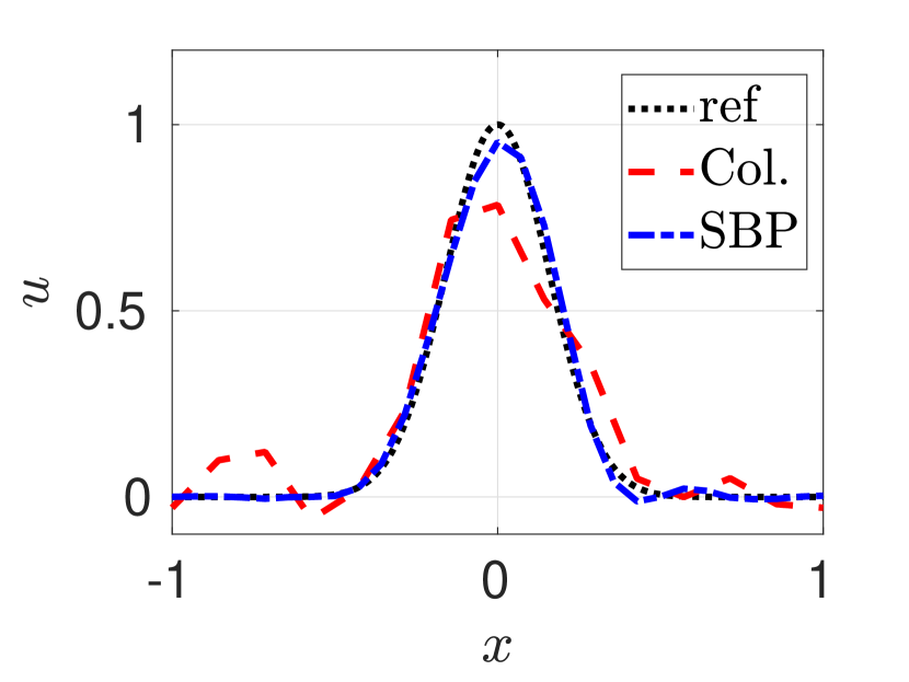
(a) $T=2$, $K=15$

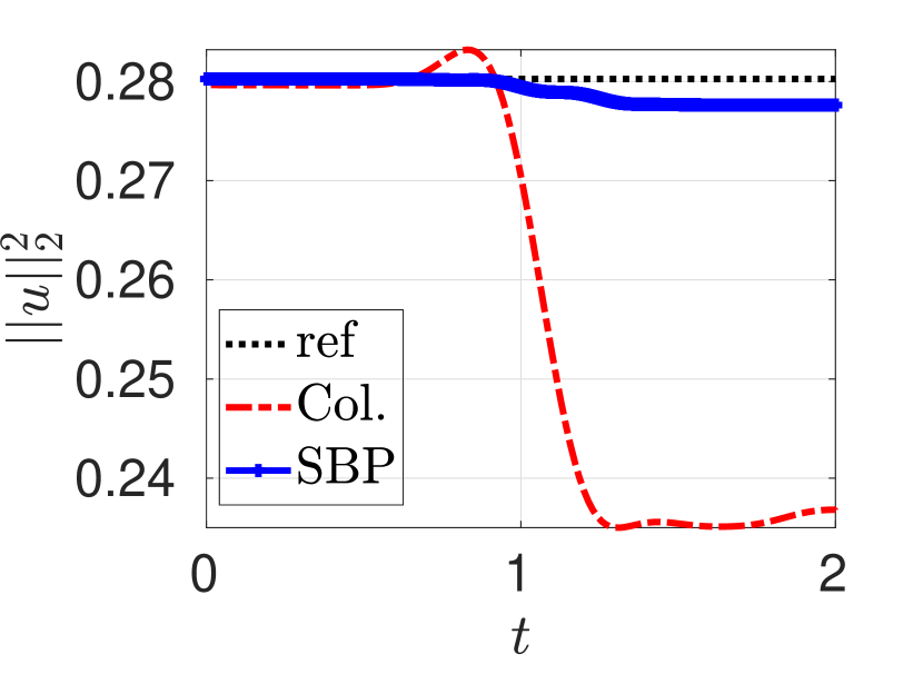
(b) $T=2$, $K=15$

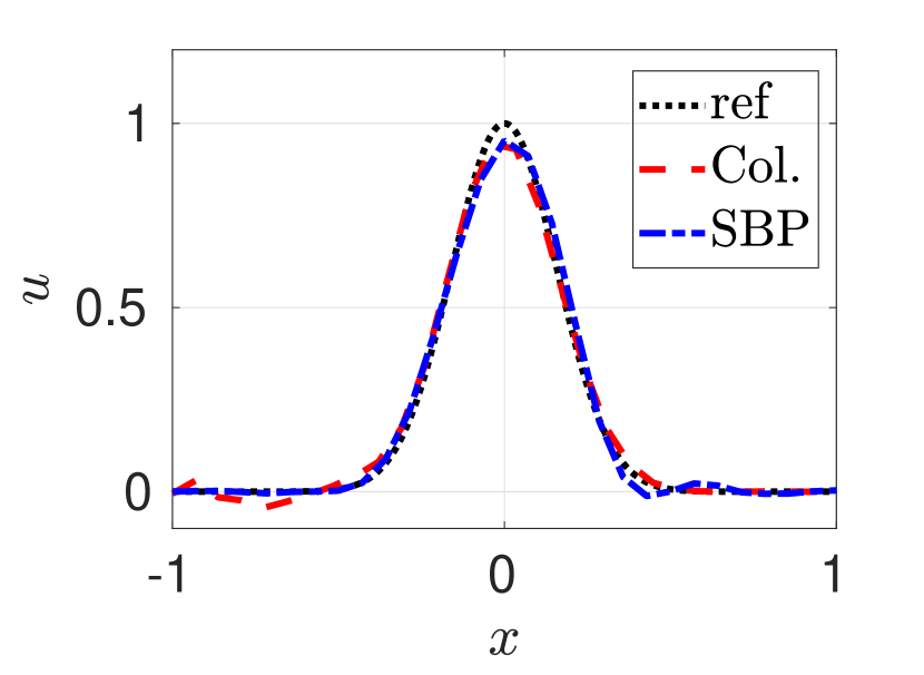
(c) $K=15/30$

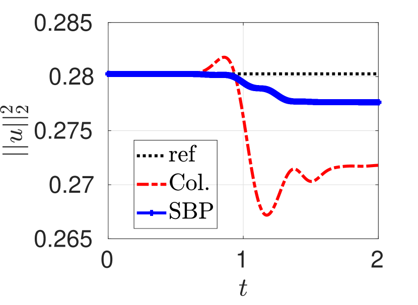
(d) $K=15/30$

Figure 2: Cubic kernels with approximation spaces $K=15/30$ on equidistant points after 1 period

Next, we focus only on RBFSBP methods and demonstrate the high accuracy of the approach by increasing the degrees of freedom. In Fig. 3, we plot the result and the energy using Gaussian ($\epsilon=1$) and cubic kernels. We use $K=5$ and $I=20$ blocks. We obtain an highly accurate solution and the energy remains constant.

(a) Numerical solution at $t=10$

(b) Energy profile developing in time

Figure 3: Gaussian and Cubic kernels with approximation space $K=5$ and $I=20$ blocks on equidistant points after 10 periods

6.2 Advection with Inflow Boundary Conditions

In the following test from [19], we consider the advection equation (37) with $a=1$ in the domain $[0,1]$. The BC and IC are

(38) $$g(t)=u_{\mathrm{init}}(0.5-t),\quad u_{\mathrm{init}}(x)=\begin{cases}\mathrm{e}^{8}\mathrm{e}^{\frac{-8}{1-(4x-1)^{2}}}&\text{if }0<x<0.5,\\ 0&\text{otherwise}.\end{cases}$$

We have a smooth IC and an inflow BC at the left boundary $x=0$. We apply cubic splines with constants as basis functions and the discretization

(39) $$\mathbf{u}_{t}+aD\mathbf{u}=P^{-1}\mathbb{S}.$$

with the simultaneous approximate terms (SAT) $\mathbb{S}\mathrel{\mathop{\ordinarycolon}}=[\mathbb{S}_{0},0,\dots,0]^{T},\quad\mathbb{S}_{0}\mathrel{\mathop{\ordinarycolon}}=-(u_{0}-g).$ In Fig. 4(a) - Fig. 4(b), we show the solutions at time t = 0.5 with $K=5$ and $I=15,20$ elements using equidistant point and randomly disturbed equidistant points. The numerical solutions using disturbed points in Fig. 4(a) has wiggles but these are reduced by increasing the number of blocks, see Fig. 4(b). Note that that the wiggles are more pronounced if the point selection is not distributed symmetrically around the midpoints, e.g. for the Halton points in Fig. 4(c) - Fig. 4(d). Next, we focus on the error behavior. As mentioned before, the RBF methods can reach spectral accuracy for smooth solutions. In Fig. 5, the error behaviour for $K=3-7$ basis functions using 20 blocks is plotted in a logarithmic scale. Spectral accuracy is indicated by the (almost) constant slope.

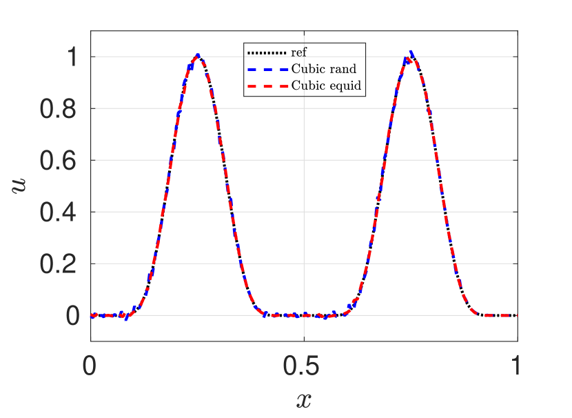
(a) $I=15$ Blocks

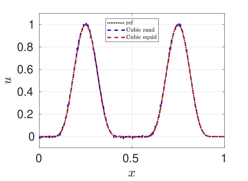
(b) I=20 Blocks,

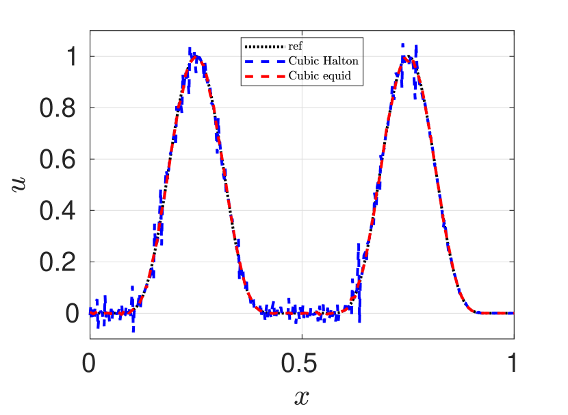
(c) $I=15$ Blocks

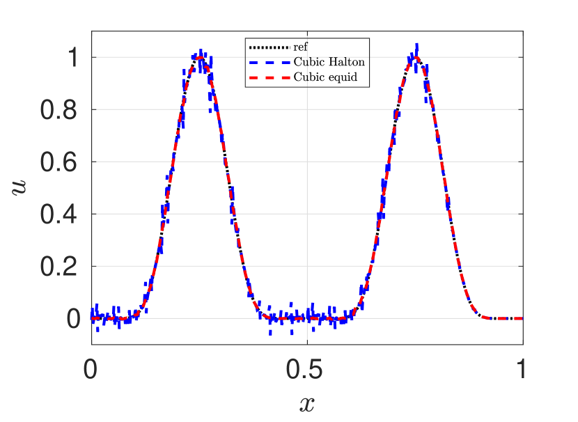
(d) I=20 Blocks,

Figure 4: Cubic kernel with approximation space $K=5$ on equidistant, and Halton points

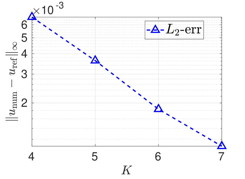
(a) $L^{2}$-error

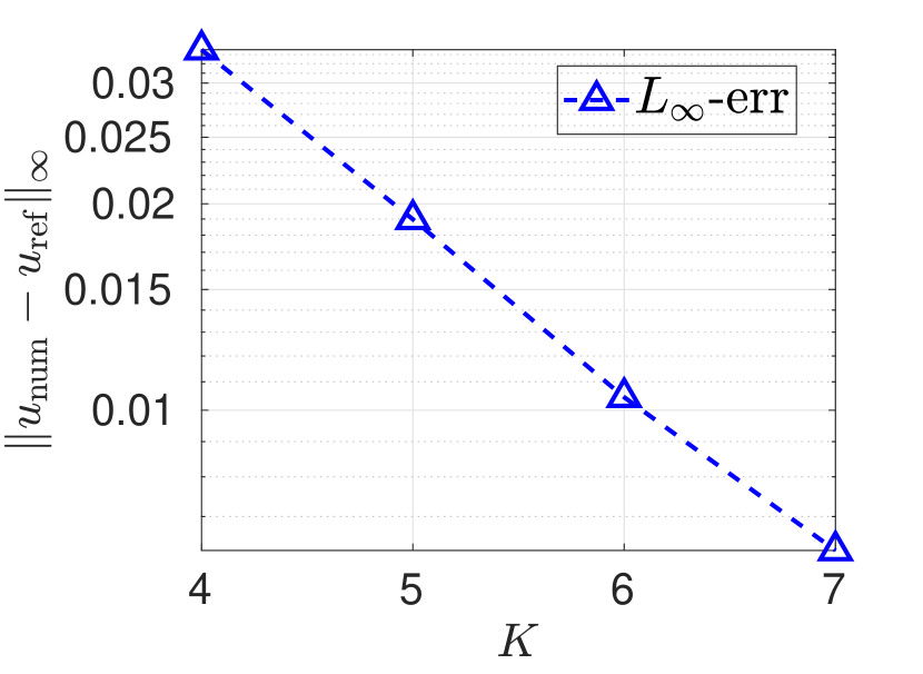
(b) Maximum error

Figure 5: Error plots using cubic kernels with approximation space $K=4-7$ on equidistant points with $I=20$ blocks. For $K=5$, the errors correspond to the solutions printed in the red dotted line on the right side of Fig. 4.

6.3 Advection-Diffusion

Next, the boundary layer problem from [44] is considered

$$\partial_{t}u+\partial_{x}u=\kappa\partial_{xx}^{2}u,\quad 0\leq x\leq 0.5,\ t>0.\\$$

The initial condition is $u(x,0)=2x$ and the boundary conditions are $u(0,t)=0$ and $u(0.5,t)=1$. The exact steady state solution is $u(x)=\frac{\exp\left(\frac{x}{\kappa}\right)-1}{\exp\left(\frac{1}{2\kappa}\right)-1}.$ Cubic splines and Gaussian kernels with shape parameter $1$ are used together with constants. We expect to obtain better results using Gaussian kernels due to structure of the steady state solution. In Fig. 6, we show the solutions for different times using $K=5$ elements on equidistant grid points with diffusion parameters $\kappa=0.2$ and $\kappa=0.1$.

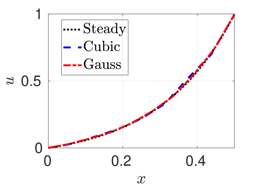
(a) $\kappa=0.2$

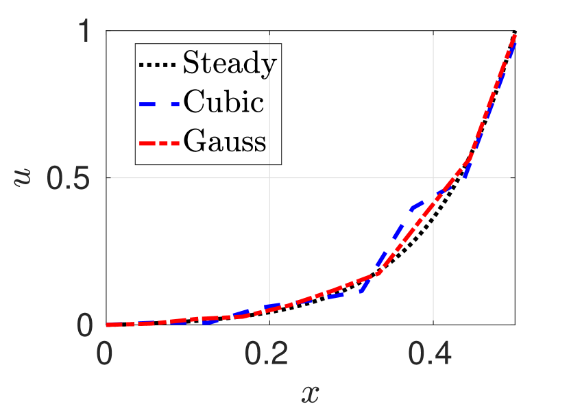
(b) $\kappa=0.1$

Figure 6: Gaussian and Cubic kernels with approximation space $K=5$ and $I=1$ block on equidistant points at $T=2$.

Some overshoots can be seen in the more steep case for $\kappa=0.1$. This behavior can be circumvented by using more degrees of freedom and multi-blocks which are avoided in this case.

6.4 2D Linear Advection

We conclude our examples with a 2D case and consider the linear advection equation:

(40) $$\partial_{t}u(x,y,t)+a\partial_{x}u(x,y,t)+b\partial_{y}u(x,y,t)=0$$

with constants $a,b\in\mathbb{R}$.

6.4.1 Periodic Boundary Conditions

In our first test, $a=b=1$ are used in (40). The initial condition is $u(x,y,0)=\mathrm{e}^{-20\left((x-0.5)^{2}+(y-0.5)^{2}\right)}$ for $(x,y)\in[0,1]^{2}$ and periodic boundary conditions, i. e., $u(0,y,t)=u(1,y,t)$ and $u(x,0,t)=u(x,1,t)$, are considered. The coupling at the boundary was again done via SAT terms. We use cubic kernels ($K=13$) equipped with constants. Fig. 7(b) illustrates the numerical solution at time $T=1$. The bump has once left the domain at the right upper corner and entered again in the left lower corner. It reaches its initial position at $T=1$. No visible differences between the numerical solution at $T=1$ and the initial condition can be seen. In Fig. 7(c) the energy is reported over time. We notice a slide decrease of energy when the bump is leaving the domain (at $t=0.5$) due to weakly enforced slightly dissipative SBP-SAT coupling.

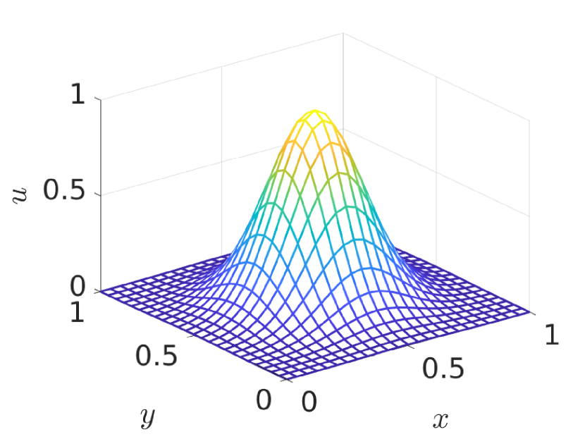
(a) Initial Condition

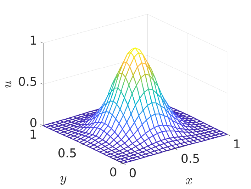
(b) Numerical Solution $T=1$

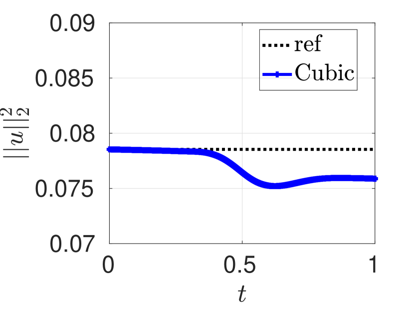
(c) Energy over $T$

Figure 7: Cubic kernels with approximation space $K=13$ on equidistant points,

6.4.2 Inflow Conditions

In the last simulation, we consider (40) with $a=0.5$, $b=1$, initial condition $u(x,y,0)=\mathrm{e}^{-20\left((x-0.25)^{2}+(y-0.25)^{2}\right)}$ for $(x,y)\in[0,1]^{2}$ and zero inflow $u(0,y,t)=0$, and $u(x,0,t)=0$. We again use cubic kernels ($K=13$) equipped with constants. The boundary conditions are enforced weakly via SAT terms. The initial condition lies in the left corner, cf. Fig. 7(a). In Fig. 8(b), the numerical solution is shown. The bump moves in $y$ direction with speed one and in $x$-direction with speed $0.5$. Fig. 8(c) shows a slight decrease of the energy over time due the bump leaving the domain.

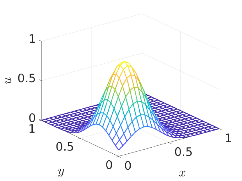
(a) Initial Condition

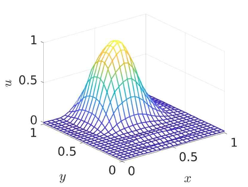
(b) Numerical Solution $T=0.5$

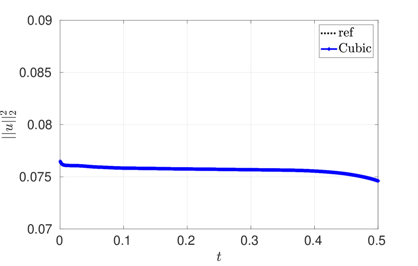
(c) Energy over $T$

Figure 8: Cubic kernels with approximation space $K=13$ on equidistant points

7 Concluding Thoughts

RBF methods are a popular tool for numerical PDEs. However, despite their success for problems with sufficient inherent dissipation, stability issues are often observed for advection-dominated problems. In this work, we used the FSBP theory combined with a weak enforcement of BCs to develop provable energy-stable RBF methods. We found that one can construct RBFSBP operators by using oversampling to obtain suitable positive quadrature formulas. Existing RBF methods do not satisfy such an RBFSBP property, either because they are based on collocation or because an inappropriate quadrature is used. Our findings imply that FSBP theory provide a building block for systematically developing stable RBF methods, filling a critical gap in the RBF theory. The focus in this paper was on global RBF methods, future works will address the extension to local RBF methods.

Appendix A Necessity of Polynomials in RBFs

For completeness, we shortly explain why the RBF interpolant Eq. 10 exists uniquely when the kernel $\varphi$ is conditionally positive definite of order $m$ and polynomials of degree up to $m-1$ are incorporated. To this end, recall that $\varphi$ is conditionally positive definite of order $m$ when

(41) $$\boldsymbol{\alpha}^{T}\Phi\boldsymbol{\alpha}>0$$

for all $\boldsymbol{\alpha}\in\mathbb{R}^{K}\setminus\{\mathbf{0}\}$ that satisfy Eq. 12, where $\Phi$ is given by Eq. 14. Further, Eq. 12 is equivalent to $P^{T}\boldsymbol{\alpha}=\mathbf{0}$. Next note that the RBF interpolant Eq. 10 exists uniquely if and only if the linear system Eq. 13 has a unique solution for every $\mathbf{u}$, which is equivalent to the corresponding homogeneous linear system

(42) $$\Phi\boldsymbol{\alpha}+P\boldsymbol{\beta} =\mathbf{0},$$

(43) $$P^{T}\boldsymbol{\alpha} =\mathbf{0},$$

admitting only the trivial solution, $\boldsymbol{\alpha}=\mathbf{0}$ and $\boldsymbol{\beta}=\mathbf{0}$. To show that this is the case, we multiply both sides of Eq. 42 by $\boldsymbol{\alpha}^{T}$ from the left, which yields

(44) $$\boldsymbol{\alpha}^{T}\Phi\boldsymbol{\alpha}=\mathbf{0},$$

since $\boldsymbol{\alpha}^{T}P=\mathbf{0}^{T}$ due to Eq. 43. Further, for conditionally positive definite $\varphi$, Eq. 44 implies $\boldsymbol{\alpha}=\mathbf{0}$. Substituting $\boldsymbol{\alpha}=\mathbf{0}$ into Eq. 42 yields $P\boldsymbol{\beta}=\mathbf{0}$, which means that the polynomial

(45) $$p(x)=\sum_{l=1}^{m}\beta_{l}p_{l}(x)$$

has zeros $x_{1},\dots,x_{K}$. Finally, for $m\leq K$, this can only be the case if $\boldsymbol{\beta}=\mathbf{0}$.

Appendix B RBFSBP property with Non-diagonal Norm Matrix

In Section 4.2, we demonstrated that there exist no diagonal $P$ such that the RBFSBP properties are fulfilled in general. In the general definition (4.1), $P$ must only be symmetric positiv definite and not necessarily diagonal. Therefore, some non-diagonal norm matrix might exists fulfilling the RBFSBP property. Here, we demonstrate that this is not the case. To investigate this, we set $X_{K}=Y_{N}$. The differentiation operators ${D\in\mathbb{R}^{N\times N}}$ of classic global RBF methods are usually constructed to be exact for the elements of the finite dimensional function space $\mathcal{R}_{m}(Y_{N})$. Unfortunately, neither the norm matrix $P$ nor the matrix $Q$ are explicitly part of RBF methods, which only come with an RBF-exact differentiation operator ${D\in\mathbb{R}^{N\times N}}$ for the cardinal functions. That said, we will now demonstrate that in many cases existing collocation RBF methods cannot satisfy the RBFSBP property since certain conditions are violated.
To this end, let ${D\in\mathbb{R}^{N\times N}}$ be the RBF-differentiation operator. We assume that there exist a positive definite and symmetric norm matrix $P\in\mathbb{R}^{N\times N}$ and a matrix $Q\in\mathbb{R}^{N\times N}$ such that (see Definition 4.1)

(46) $$D=P^{-1}Q,\quad Q+Q^{T}=B.$$

The two conditions in Eq. 46 can be combined to

(47) $$PD+(PD)^{T}-B=0.$$

Next, we assume that the RBF interpolant include polynomials of most degree $m-1\geq 0$. In this case, $\mathcal{R}_{1}(Y_{N})$ contains constants and $P$ must be associated with a $\mathcal{R}_{1}(Y_{N})$-exact quadrature formula. Since $D$ is $\mathcal{R}_{1}(Y_{N})$-exact, this can be reformulated as

(48) $$\int_{x_{L}}^{x_{R}}1\partial_{x}fdx=f|_{x_{L}}^{x_{R}}\Longleftrightarrow\mathbf{1}^{T}PD\mathbf{f}=f|_{x_{L}}^{x_{R}}\quad\forall f\in\mathcal{R}_{1}(Y_{N})$$

Since $D$ and $\mathbf{f}$ are formulated with respect to the same basis $\mathrm{span}\{c_{k}\}$. The entries of $D$ are given by $D_{jk}=c_{k}^{\prime}(x_{j})$ with collocation points $x_{j}$. Hence, (48) is used for every basis element $\mathrm{span}\{c_{i}\}$, e.g. for $c_{1}$:

(49) $$c_{1}|_{x_{L}}^{x_{R}}=c_{1}(x_{R})-c_{1}(x_{L})=\int_{x_{L}}^{x_{R}}1\partial_{x}c_{1}dx=\sum_{j=1}^{N}w_{j}c^{\prime}_{1}(x_{j})=\mathbf{1}^{T}P\mathbf{c_{1}^{\prime}}.$$

Since $\mathbf{c_{i}^{\prime}}$ are the columns of the derivative matrix. We can collect every basis element using (49) resulting in

(50) $$\mathbf{1}^{T}PD=\mathbf{m}.$$

with $\mathbf{m}=[c_{1}|_{x_{L}}^{x_{R}},\dots,c_{N}|_{x_{L}}^{x_{R}}]$. We shall now summarize the above discussion: Let $m-1\geq 0$ and ${b(P)\mathrel{\mathop{\ordinarycolon}}=\|PD+(PD)^{T}-B\|_{2}}$. Moreover, for given $D$ let us consider the following optimization problem:

(51) $$\min_{P}\left\{\,b(P)\ \text{ s.t. }\ P=P^{T},\ P>0,\ \mathbf{1}^{T}PD=\mathbf{m}\,\right\}$$

If the differentiation operator $D$ of a classic global RBF method satisfies the FSBP property, then minimizers $P^{*}$ of the optimization problem Eq. 51 satisfy $b(P^{*})=0$. There exist a suitable quadrature formula to determine $P$ through the minimization problem (51). It should be stressed that $b(P)=0$ is necessary for the given $D$ to satisfy the SBP property, but not sufficient. This follows directly from [20, Lemma 4.3] containing the fact that the derivatives of the basis functions are integrated exactly.

Equidistant points
		cubic				quintic
$N$/$m-1$		$0$	$1$	$2$		$0$	$1$	$2$
$10$		$1.5e-10$	$8.1e-11$	$5.8e-10$		$5.8e-10$	$4.0e-10$	$4.0e-10$
$20$		$3.8e-10$	$9.3e-10$	$5.5e-10$		$1.0e-05$	$7.5e-08$	$6.0e-08$

Halton points
		cubic				quintic
$N$/$m-1$		$-1$	$0$	$1$		$-1$	$0$	$1$
$10$		$1.8e-01$	$2.0e-01$	$2.0e-01$		$3.1e-01$	$1.9e-01$	$1.8e-01$
$20$		$1.9e-01$	$2.0e-01$	$1.9e-01$		$1.8e-01$	$1.6e-01$	$1.5e-01$

Random points
		cubic				quintic
$N$/$m-1$		$-1$	$0$	$1$		$-1$	$0$	$1$
$10$		$1.2e-01$	$9.3e-02$	$1.0e-01$		$9.3e-01$	$5.9e-01$	$5.7e-01$
$20$		$6.9e-02$	$7.1e-02$	$6.4e-02$		$3.2e+02$	$5.1e+00$	$3.6e-01$

Table 3: Residual $\|PD+(PD)^{T}-B\|_{2}$ for the determined norm matrix $P$ in the case of equidistant, Halton, and random grid points

In our implementation we solved Eq. 51 using Matlab’s CVX [22]. The results for different numbers and types of grid points $\mathbf{x}$ as well as kernels $\varphi$ and polynomial degrees $m-1$ can be found in Table 3. Our numerical findings indicate that in all cases classic global RBF methods do not satisfy the RBFSBP property. This can be noted from the residual $b(P)=\|PD+(DP)^{T}-B\|_{2}$ corresponding to the minimizer $P$ of Eq. 51 to be distinctly different from zero (machine precision in our implementation is around $10^{-16}$). This result is not suprising and in accordance with the observations made in the literature [18, 41].

References

- [1] R. Abgrall, J. Nordström, P. Öffner, and S. Tokareva, Analysis of the SBP-SAT stabilization for finite element methods I: Linear problems, J. Sci. Comput., 85 (2020), p. 28, https://doi.org/10.1007/s10915-020-01349-z. Id/No 43.
- [2] R. Abgrall, J. Nordström, P. Öffner, and S. Tokareva, Analysis of the SBP-SAT stabilization for finite element methods part ii: Entropy stability, Communications on Applied Mathematics and Computation, (2021), pp. 1–23.
- [3] M. H. Carpenter, J. Nordström, and D. Gottlieb, Revisiting and extending interface penalties for multi-domain summation-by-parts operators, J. Sci. Comput., 45 (2010), pp. 118–150, https://doi.org/10.1007/s10915-009-9301-5.
- [4] J. Chan, D. C. Del Rey Fernández, and M. H. Carpenter, Efficient entropy stable Gauss collocation methods, SIAM J. Sci. Comput., 41 (2019), pp. a2938–a2966, https://doi.org/10.1137/18M1209234.
- [5] S. Cuomo, F. Sica, and G. Toraldo, Greeks computation in the option pricing problem by means of RBF-PU methods, J. Comput. Appl. Math., 376 (2020), p. 14, https://doi.org/10.1016/j.cam.2020.112882. Id/No 112882.
- [6] M. Dehghan and V. Mohammadi, A numerical scheme based on radial basis function finite difference (RBF-FD) technique for solving the high-dimensional nonlinear Schrödinger equations using an explicit time discretization: Runge–Kutta method, Computer Physics Communications, 217 (2017), pp. 23–34.
- [7] D. C. Del Rey Fernández, J. E. Hicken, and D. W. Zingg, Review of summation-by-parts operators with simultaneous approximation terms for the numerical solution of partial differential equations, Comput. Fluids, 95 (2014), pp. 171–196, https://doi.org/10.1016/j.compfluid.2014.02.016.
- [8] G. E. Fasshauer, Meshfree Approximation Methods with MATLAB, vol. 6, World Scientific, 2007.
- [9] N. Flyer, B. Fornberg, V. Bayona, and G. A. Barnett, On the role of polynomials in RBF-FD approximations. I: Interpolation and accuracy, J. Comput. Phys., 321 (2016), pp. 21–38, https://doi.org/10.1016/j.jcp.2016.05.026.
- [10] N. Flyer, E. Lehto, S. Blaise, G. B. Wright, and A. St-Cyr, A guide to RBF-generated finite differences for nonlinear transport: shallow water simulations on a sphere, J. Comput. Phys., 231 (2012), pp. 4078–4095, https://doi.org/10.1016/j.jcp.2012.01.028.
- [11] B. Fornberg and N. Flyer, Accuracy of radial basis function interpolation and derivative approximations on 1-D infinite grids, Advances in Computational Mathematics, 23 (2005), pp. 5–20.
- [12] B. Fornberg and N. Flyer, A Primer on Radial Basis Functions With Applications to the Geosciences, SIAM, 2015.
- [13] B. Fornberg, E. Larsson, and N. Flyer, Stable computations with gaussian radial basis functions, SIAM Journal on Scientific Computing, 33 (2011), pp. 869–892.
- [14] G. J. Gassner, A. R. Winters, and D. A. Kopriva, Split form nodal discontinuous Galerkin schemes with summation-by-parts property for the compressible Euler equations, J. Comput. Phys., 327 (2016), pp. 39–66, https://doi.org/10.1016/j.jcp.2016.09.013.
- [15] J. Glaubitz, Shock Capturing and High-Order Methods for Hyperbolic Conservation Laws, Logos Verlag Berlin GmbH, 2020.
- [16] J. Glaubitz, Stable high order quadrature rules for scattered data and general weight functions, SIAM J. Numer. Anal., 58 (2020), pp. 2144–2164, https://doi.org/10.1137/19M1257901.
- [17] J. Glaubitz, Construction and application of provable positive and exact cubature formulas, IMA Journal of Numerical Analysis, (2022), https://arxiv.org/abs/2108.02848. To appear.
- [18] J. Glaubitz and A. Gelb, Stabilizing radial basis function methods for conservation laws using weakly enforced boundary conditions, J. Sci. Comput., 87 (2021), p. 29, https://doi.org/10.1007/s10915-021-01453-8. Id/No 40.
- [19] J. Glaubitz, E. Le Meledo, and P. Öffner, Towards stable radial basis function methods for linear advection problems, Comput. Math. Appl., 85 (2021), pp. 84–97, https://doi.org/10.1016/j.camwa.2021.01.012.
- [20] J. Glaubitz, J. Nordström, and P. Öffner, Summation-by-parts operators for general approximation spaces, arXiv preprint arXiv: 2203.05479, (2022).
- [21] J. Gong and J. Nordström, Interface procedures for finite difference approximations of the advection-diffusion equation, J. Comput. Appl. Math., 236 (2011), pp. 602–620, https://doi.org/10.1016/j.cam.2011.08.009.
- [22] M. Grant and S. Boyd, CVX: Matlab software for disciplined convex programming, 2014. Version 2.2.
- [23] B. Gustafsson, H.-O. Kreiss, and J. Oliger, Time dependent problems and difference methods, vol. 24, John Wiley & Sons, 1995.
- [24] J. S. Hesthaven, F. Mönkeberg, and S. Zaninelli, RBF based CWENO method, in Spectral and high order methods for partial differential equations, ICOSAHOM 2018. Selected papers from the ICOSAHOM conference, London, UK, July 9–13, 2018, Cham: Springer, 2020, pp. 191–201, https://doi.org/10.1007/978-3-030-39647-3_14.
- [25] A. Iske, Ten good reasons for using polyharmonic spline reconstruction in particle fluid flow simulations, Continuum Mechanics, Applied Mathematics and Scientific Computing: Godunov’s Legacy, (2020), pp. 193–199.
- [26] E. J. Kansa, Multiquadrics – a scattered data approximation scheme with applications to computational fluid-dynamics. II: Solutions to parabolic, hyperbolic and elliptic partial differential equations, Comput. Math. Appl., 19 (1990), pp. 147–161, https://doi.org/10.1016/0898-1221(90)90271-K.
- [27] A. Kitson, R. I. McLachlan, and N. Robidoux, Skew-adjoint finite difference methods on nonuniform grids, New Zealand J. Math, 32 (2003), pp. 139–159.
- [28] D. Lazzaro and L. B. Montefusco, Radial basis functions for the multivariate interpolation of large scattered data sets, J. Comput. Appl. Math., 140 (2002), pp. 521–536, https://doi.org/10.1016/S0377-0427(01)00485-X.
- [29] V. Linders, J. Nordström, and S. H. Frankel, Properties of Runge-Kutta-summation-by-parts methods, Journal of Computational Physics, 419 (2020), p. 109684.
- [30] J. Nordström, Conservative finite difference formulations, variable coefficients, energy estimates and artificial dissipation, J. Sci. Comput., 29 (2006), pp. 375–404, https://doi.org/10.1007/s10915-005-9013-4.
- [31] J. Nordström, A roadmap to well posed and stable problems in computational physics, J. Sci. Comput., 71 (2017), pp. 365–385, https://doi.org/10.1007/s10915-016-0303-9.
- [32] P. Öffner and H. Ranocha, Error boundedness of discontinuous Galerkin methods with variable coefficients, J. Sci. Comput., 79 (2019), pp. 1572–1607, https://doi.org/10.1007/s10915-018-00902-1.
- [33] U. Pettersson, E. Larsson, G. Marcusson, and J. Persson, Improved radial basis function methods for multi-dimensional option pricing, J. Comput. Appl. Math., 222 (2008), pp. 82–93, https://doi.org/10.1016/j.cam.2007.10.038.
- [34] R. B. Platte and T. A. Driscoll, Eigenvalue stability of radial basis function discretizations for time-dependent problems, Comput. Math. Appl., 51 (2006), pp. 1251–1268, https://doi.org/10.1016/j.camwa.2006.04.007.
- [35] H. Ranocha, P. Öffner, and T. Sonar, Extended skew-symmetric form for summation-by-parts operators and varying Jacobians, J. Comput. Phys., 342 (2017), pp. 13–28, https://doi.org/10.1016/j.jcp.2017.04.044.
- [36] C. Shu, Total-variation-diminishing time discretizations, SIAM J. Sci. Stat. Comput., 9 (1988), pp. 1073–1084, https://doi.org/10.1137/0909073.
- [37] M. Svärd, On coordinate transformations for summation-by-parts operators, J. Sci. Comput., 20 (2004), pp. 29–42, https://doi.org/10.1023/A:1025881528802.
- [38] M. Svärd and J. Nordström, Review of summation-by-parts schemes for initial-boundary-value problems, J. Comput. Phys., 268 (2014), pp. 17–38, https://doi.org/10.1016/j.jcp.2014.02.031.
- [39] A. I. Tolstykh, On using RBF-based differencing formulas for unstructured and mixed structured-unstructured grid calculations, in Proceedings of the 16th IMACS world congress, vol. 228, Lausanne, 2000, pp. 4606–4624.
- [40] I. Tominec and M. Nazarov, Residual viscosity stabilized RBF-FD methods for solving nonlinear conservation laws, arXiv preprint arXiv:2109.07183, (2021).
- [41] I. Tominec, M. Nazarov, and E. Larsson, Stability estimates for radial basis function methods applied to time-dependent hyperbolic PDEs, arXiv preprint arXiv:2110.14548, (2021).
- [42] H. Wendland, Fast evaluation of radial basis functions: Methods based on partition of unity, in Approximation Theory X: Wavelets, Splines, and Applications, Citeseer, 2002.
- [43] H. Wendland, Scattered Data Approximation, vol. 17, Cambridge University Press, 2004.
- [44] L. Yuan and C.-W. Shu, Discontinuous Galerkin method based on non-polynomial approximation spaces, J. Comput. Phys., 218 (2006), pp. 295–323, https://doi.org/10.1016/j.jcp.2006.02.013.