Visibility, invisibility and unique recovery of inverse electromagnetic problems with conical singularities

Abstract.

In this paper, we study time-harmonic electromagnetic scattering in two scenarios, where the anomalous scatterer is either a pair of electromagnetic sources or an inhomogeneous medium, both with compact supports. We are mainly concerned with the geometrical inverse scattering problem of recovering the support of the scatterer, independent of its physical contents, by a single far-field measurement. It is assumed that the support of the scatterer (locally) possesses a conical singularity. We establish a local characterisation of the scatterer when invisibility/transparency occurs, showing that its characteristic parameters must vanish locally around the conical point. Using this characterisation, we establish several local and global uniqueness results for the aforementioned inverse scattering problems, showing that visibility must imply unique recovery. In the process, we also establish the local vanishing property of the electromagnetic transmission eigenfunctions around a conical point under the Hölder regularity or a regularity condition in terms of Herglotz approximation.

Keywords:  electromagnetic waves, geometrical inverse scattering, conical singularity, invisibility and transparency, locally vanishing, unique recovery, single far-field measurement, transmission eigenfunctions.

2010 Mathematics Subject Classification:  78A45, 35Q61, 35P25 (primary); 78A46, 35P25, 35R30 (secondary).

1. Introduction

In this paper, we study time-harmonic electromagnetic scattering in two scenarios, where the anomalous scatterer is either a pair of electromagnetic sources or an inhomogeneous medium, both with compact supports. We first introduce the forward scattering problems in the two scenarios.

Let $\Omega$ be a bounded Lipschitz domain in $\mathbb{R}^{3}$ with a connected complement $\mathbb{R}^{3}\backslash\overline{\Omega}$, which signifies the support of an inhomogeneous scatterer. Let $\mathbf{J}_{j}(\mathbf{x})$, $\mathbf{x}\in\mathbb{R}^{3}$ and $j=1,2$, be $\mathbb{C}^{3}$-valued functions such that $\mathrm{supp}(\mathbf{J}_{j})\subset\Omega$. It is assumed that $\mathbf{J}_{1}|_{\Omega}\in L^{2}(\Omega;\mathbb{C}^{3})$ and $\mathbf{J}_{2}|_{\Omega}\in L^{2}(\Omega;\mathbb{C}^{3})$, which signify the intensities of active electric and magnetic sources, respectively. Let $(\mathbf{E},\mathbf{H})\in H_{\mathrm{loc}}(\mathrm{curl},\mathbb{R}^{3})\times H_{\mathrm{loc}}(\mathrm{curl},\mathbb{R}^{3})$ denote the electric and magnetic fields respectively. Consider the following electromagnetic scattering problem

$$\begin{cases}&\nabla\wedge\mathbf{E}(\mathbf{x})-\mathrm{i}\omega\mu_{0}\mathbf{H}(\mathbf{x})=\mathbf{J}_{1}(\mathbf{x}),\quad\mathbf{x}\in\mathbb{R}^{3},\\ &\nabla\wedge\mathbf{H}(\mathbf{x})+\mathrm{i}\omega\varepsilon_{0}\mathbf{E}(\mathbf{x})=\mathbf{J}_{2}(\mathbf{x}),\quad\,\mathbf{x}\in\mathbb{R}^{3},\\ &\lim_{|\mathbf{x}|\to\infty}|\mathbf{x}|\left({\mu}_{0}^{1/2}\mathbf{H}\times\frac{\mathbf{x}}{|\mathbf{x}|}-{\varepsilon}_{0}^{1/2}\mathbf{E}\right)=0,\end{cases}$$ (1.1)

where $\omega\in\mathbb{R}_{+}$ signifies the frequency of the wave, and $\varepsilon_{0}$ and $\mu_{0}\in\mathbb{R}_{+}$, respectively, denote the electric permittivity and magnetic permeability of a uniformly homogeneous space. The last limit in (1.1) is known as the Silver-Müller radiation condition which holds uniformly in all directions $\hat{\mathbf{x}}:=\mathbf{x}/|\mathbf{x}|\in\mathbb{S}^{2}$, $\mathbf{x}\in\mathbb{R}^{3}\setminus\{\mathbf{0}\}$, and characterizes the outgoing nature of the electromagnetic waves. It is emphasized that we consider the possible presence of both electric and magnetic sources, though only the electric source might be the physically meaningful one. The well-posedness of the Maxwell system (1.1) can be conveniently found in [26, 32]. We know that as $|{\mathbf{x}}|\rightarrow+\infty$ it holds that

$$\left(\mathbf{E},\mathbf{H}\right)(\mathbf{x})=\frac{e^{\mathrm{i}k|\mathbf{x}|}}{|\mathbf{x}|}\left(\mathbf{E}_{\infty},\mathbf{H}_{\infty}\right)(\hat{\mathbf{x}})+\mathcal{O}\left(\frac{1}{|\mathbf{x}|^{2}}\right),$$ (1.2)

where $k:=\omega\sqrt{\varepsilon_{0}\mu_{0}}$ is known as the wavenumber, and $\mathbf{E}_{\infty}(\hat{\mathbf{x}})$ and $\mathbf{H}_{\infty}(\hat{\mathbf{x}})$ are referred to the electric and the magnetic far-field patterns respectively. It is known that $\mathbf{E}_{\infty}$ and $\mathbf{H}_{\infty}$ are analytic functions on the unit sphere $\mathbb{S}^{2}$ with the following one-to-one correspondence

$$\mathbf{H}_{\infty}(\hat{\mathbf{x}})=\hat{\mathbf{x}}\wedge\mathbf{E}_{\infty}(\hat{\mathbf{x}})\quad\text{and}\quad\mathbf{E}_{\infty}(\hat{\mathbf{x}})=-\hat{\mathbf{x}}\wedge\mathbf{H}_{\infty}(\hat{\mathbf{x}}),\quad\ \ \forall\hat{\mathbf{x}}\in\mathbb{S}^{2}.$$ (1.3)

Next we introduce the scattering due to the interaction of a (passive) inhomogeneous medium scatterer and an (actively sent) incident wave. Suppose that $\Omega$ supports an inhomogeneous medium whose material parameters are characterised by the electric permittivity $\varepsilon\in L^{\infty}(\Omega;\mathbb{R}_{+})$, magnetic permeability $\mu\in L^{\infty}(\Omega;\mathbb{R}_{+})$ and electric conductivity $\sigma\in L^{\infty}(\Omega;\mathbb{R}_{+}^{0})$. Throughout the rest of the paper, we set

$$\varepsilon(\mathbf{x})=\begin{cases}\varepsilon_{0},\ \mathbf{x}\in\mathbb{R}^{3}\setminus\overline{\Omega},\\ \varepsilon,\ \ \mathbf{x}\in\Omega,\end{cases},\ \mu(\mathbf{x})=\begin{cases}\mu_{0},\ \mathbf{x}\in\mathbb{R}^{3}\setminus\overline{\Omega},\\ \mu,\ \ \mathbf{x}\in\Omega,\end{cases},\ \sigma(\mathbf{x})=\begin{cases}0,\ \mathbf{x}\in\mathbb{R}^{3}\setminus\overline{\Omega},\\ \sigma,\ \mathbf{x}\in\Omega.\end{cases}$$

The incident wave field $(\mathbf{E}^{i},\mathbf{H}^{i})$ is a pair of entire solutions to

$$\nabla\wedge\mathbf{E}^{i}-\mathrm{i}\omega\mu_{0}\mathbf{H}^{i}=\mathbf{0},\quad\nabla\wedge\mathbf{H}^{i}+\mathrm{i}\omega\varepsilon_{0}\mathbf{E}^{i}=\mathbf{0}\quad\mbox{in}\ \ \mathbb{R}^{3},$$ (1.4)

which interacts with the scattering medium described above. The resulting scattered electromagnetic wave field is denoted by $(\mathbf{E},\mathbf{H})$. Hence the total electromagnetic wave field $(\mathbf{E}^{t},\mathbf{H}^{t})$ is the superposition of the incident and scattered waves, i.e.,

$$(\mathbf{E}^{t},\mathbf{H}^{t})=(\mathbf{E}^{i},\mathbf{H}^{i})+(\mathbf{E},\mathbf{H})\quad\mbox{in}\ \ \mathbb{R}^{3}.$$

The aforementioned electromagnetic scattering can be modelled by the following Maxwell system

$$\begin{cases}&\nabla\wedge\mathbf{E}^{t}({\mathbf{x}})-\mathrm{i}\omega\mu({\mathbf{x}})\mathbf{H}^{t}({\mathbf{x}})=0,\hskip 51.21504pt{\mathbf{x}}\in\mathbb{R}^{3},\vskip 6.0pt plus 2.0pt minus 2.0pt\\ &\nabla\wedge\mathbf{H}^{t}({\mathbf{x}})+\mathrm{i}\omega\gamma({\mathbf{x}})\mathbf{E}^{t}({\mathbf{x}})=0,\hskip 51.21504pt{\mathbf{x}}\in\mathbb{R}^{3},\vskip 6.0pt plus 2.0pt minus 2.0pt\\ &\lim_{|\mathbf{x}|\to\infty}|\mathbf{x}|\left({\mu}_{0}^{1/2}\mathbf{H}\times\frac{\mathbf{x}}{|\mathbf{x}|}-{\varepsilon}_{0}^{1/2}\mathbf{E}\right)=0.\end{cases}$$ (1.5)

where $\gamma(\mathbf{x})=\varepsilon(\mathbf{x})+\mathrm{i}\sigma(\mathbf{x})/\omega$. The well-posedness of (1.5) can be found in [26, 32], which guarantees the unique existence of a pair of solutions $(\mathbf{E},\mathbf{H})\in H_{\mathrm{loc}}(\mathrm{curl},\mathbb{R}^{3})\times H_{\mathrm{loc}}(\mathrm{curl},\mathbb{R}^{3})$ to (1.5). Furthermore, the scattered electromagnetic waves $\left(\mathbf{E},\mathbf{H}\right)$ have the following asymptotic expansion:

$$\left(\mathbf{E},\mathbf{H}\right)(\mathbf{x})=\frac{e^{\mathrm{i}k|\mathbf{x}|}}{|\mathbf{x}|}\left(\mathbf{E}_{\infty},\mathbf{H}_{\infty}\right)(\hat{\mathbf{x}})+\mathcal{O}\left(\frac{1}{|\mathbf{x}|^{2}}\right).$$ (1.6)

Henceforth, we write $(\Omega;\mathbf{J}_{1},\mathbf{J}_{2})$ and $(\Omega;\varepsilon,\mu,\sigma)$ to denote the source and medium scatterers respectively introduced above. Here, $\Omega$ signifies the support of the scatterer which contains its shape and location information, whereas $\mathbf{J}_{1},\mathbf{J}_{2}$ or $\varepsilon,\mu,\sigma$ are its physical content, and hereafter are referred to as the characteristic parameters of the scatterer. In the case that $\Omega$ is a medium scatterer, we also include the incident field $(\mathbf{E}^{i},\mathbf{H}^{i})$ as characteristic parameter since its interaction with the medium parameters generates the source that produces the radiating scattered waves. In this paper, one of the major concerns is the following geometrical inverse scattering problem:

$$\mathbf{E}_{\infty}(\hat{\mathbf{x}}),\ \hat{\mathbf{x}}\in\mathbb{S}^{2}\mbox{ or }\mathbf{H}_{\infty}(\hat{\mathbf{x}}),\ \hat{\mathbf{x}}\in\mathbb{S}^{2}\longmapsto\Omega\ \ \mbox{independent of its physical content},$$ (1.7)

where $\mathbf{E}_{\infty}$ (or, equivalently $\mathbf{H}_{\infty}$ by virtue of (1.3)) is either from (1.2) for the source scattering or (1.6) for the medium scattering. It is straightforwardly verified that the inverse problem (1.7) is nonlinear, though the forward scattering problem is linear. Throughout our study, it is assumed for (1.7) that $\omega\in\mathbb{R}_{+}$ is fixed and in case $\Omega$ is a medium scatterer, the far-field pattern in (1.7) is collected corresponding to a single incident wave field $(\mathbf{E}^{i},\mathbf{H}^{i})$. In such a case, $\mathbf{E}_{\infty}$ is referred to as a single far-field measurement. Clearly, in order to determine $\Omega$, it is sufficient to recover $\partial\Omega$. It can be seen that the inverse problem (1.7) is formally determined with a single far-field measurement since both $\mathbb{S}^{2}$ and $\partial\Omega$ are two-dimensional manifolds. The geometrical inverse problem (1.7) is a well-known longstanding one in the inverse scattering theory [15, 25, 30], with a colourful history and yet still largely open. It lays the theoretical foundation for many wave imaging technologies including radar, medical imaging and non-destructive testing where one is more interested in extracting the geometrical information of the anomalies by limited measurement data.

In respect to (1.7), a closely related problem is the occurrence of invisibility/transparency, namely $\mathbf{E}_{\infty}=\mathbf{H}_{\infty}\equiv\mathbf{0}$. In such case, $(\Omega;\mathbf{J}_{1},\mathbf{J}_{2})$ is said to be a non-radiating/raditioneless source and $(\Omega;\varepsilon,\mu,\sigma)$ is said to be a transparent/invisible scatterer. Recently, geometrical characterisations of non-radiating sources and transparent/invisible mediums have received considerable interest in the literature; see [2, 4, 5, 10, 12, 13, 16, 19, 24, 33, 34, 35] for related studies in acoustic scattering, [3, 20] in elastic scattering and [8, 22, 28] in electromagnetic scattering. Roughly speaking, if the support of the scatterer possesses a certain geometrical singularity on its boundary $\partial\Omega$, say e.g. a corner, then the characteristic parameters of an invisible scatter must be vanishing (locally) around the geometrical singular point. As a direct consequence, if the characteristic parameters of a scatterer is a-priori known to be non-vanishing around a geometrically singular point, then it must radiate a nontrivial scattering pattern, namely it must be visible with respect to far-field measurement. It is emphasized that this point has been essentially implied in all of the aforementioned studies on characterising radiating/non-radiating scatterers, though it may appear in different phrasings. It is also noted that in [7], a smooth boundary point with a sufficiently high curvature is shown to possess a similar characterisation as above in the context of acoustic scattering. In the current article, we make a novel contribution along the line by establishing the local vanishing property for the electromagnetic scattering in the two scenarios introduced earlier when the scatterer possesses a conical singularity. It is noted that in the context of electromagnetic scattering, only polyhedral singularities have been considered due to the highly complicated physical and technical nature. The main results on this aspect are contained in Theorems  2.2 and 3.1, respectively, for the source and medium scattering.

If visibility is guaranteed, namely the scatterer does generate scattering information to the far-field observer, the next issue of primary importance to (1.7) is the unique identifiability. That is, if there are two scatterers $\Omega$ and $\Omega^{\prime}$, with possibly different and not a-priori known physical contents, which generate the same far-field measurement if and only if $\Omega=\Omega^{\prime}$. By using the geometrical characterisation discussed above for non-radiating/transparent scatterers, we establish several novel local and global unique recovery results for (1.7), showing that visibility is equivalent to unique recovery. It is clear that for the inverse problem (1.7), visibility, i.e. $\mathbf{E}_{\infty}$ is not identically zero, does not necessarily imply unique identifiability. In our study, we can achieve such an equivalence relation due to the fact that our analysis is localised around the conical point. It is interesting to note that our global recovery results contain a special case that the scatterer is of coronal shape (cf. Fig. 1 for a schematic illustration), which may be of practical interest to the medical imaging. Finally, we would like to mention in passing some related results on uniqueness for geometrical inverse electromagnetic problems by a single far-field measurement [8, 23, 26, 29].

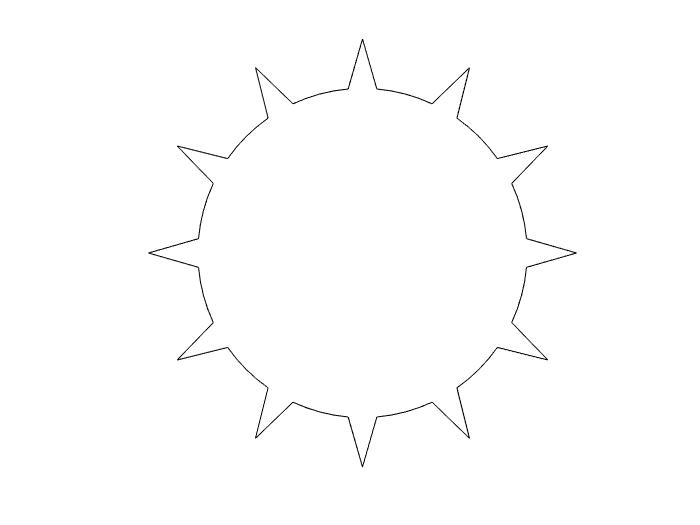
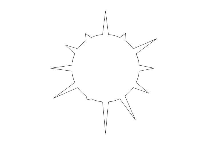
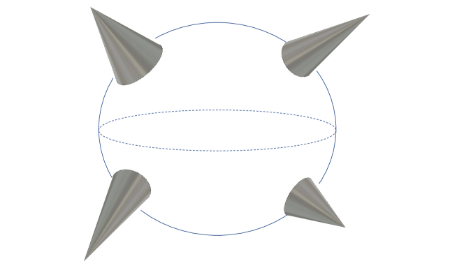
Figure 1. Schematic illustration of coronal-shape scatterers. Rigorous definition is provided in Definition 2.2. The first two are the slice plottings of two coronal-shape scatterers with many conical singularities and the third one is a 3D plotting with 4 conical singularities on its body.

Finally, we also achieve a geometrical characterisation of electromagnetic transmission eigenfunctions, showing that they must vanish (locally) around a conical point. Transmission eigenvalue problems arise from non-scattering/invisibility but go beyond, especially when the regularity of transmission eigenfunctions is weakened; see Section 4 for more related background discussion. Recently, the spectral geometry of transmission eigenfunctions has also received considerable attention in the literature; see [2, 3, 6, 7, 9, 13, 19, 20] in different physical context and especially [8, 22] in the context of electromagnetic scattering for local structures and [14, 17, 18] for global structures. We establish a local vanishing property of the electromagnetic transmission eigenfunctions around a conical point under the Hölder regularity or a regularity condition in terms of Herglotz approximation, which add a novel contribution to the spectral theory of transmission eigenfunctions.

According to our discussion above, the visibility, invisibility and unique recovery of the inverse electromagnetic problem (1.7) as well as spectral geometry of transmission eigenfunctions are separate but intriguingly connected topics. We present all those geometrical results as discussed above to corroborate the interesting connections among them. Finally, we would like to briefly discuss the mathematical strategy in establishing those geometrical results. We shall make essential use of tools from microlocal analysis to carefully analyse the singularity behaviour of the solution to the Maxwell system induced by the geometrical singularity of the shape of the underlying scatterer. This shares a similar spirit to [8] which deals with a polyhedral corner. Nevertheless, we achieve several new technical developments in order cope with the different geometrical setup as well as several other issues, especially to significantly weaken the regularity assumptions needed in [8], and make the study more physically relevant.

The rest of the paper is organised as follows. In Section 2, we consider the geometrical characterisation of non-radiating sources as well as the geometrical inverse problem (1.7) in determining the support of a source scatterer. In Section 3, we consider the geometrical characterisation of transparent/invisible medium scatterers as well as the geometrical inverse problem (1.7) in determining the support of a medium scatterer. Section 4 is devoted to the geometrical characterisation of electromagnetic transmission eigenfunctions.

2. Non-radiating sources and inverse source scattering

In this section, we establish the vanishing property of non-radiating electromagnetic sources around a conical corner, and then use it to derive unique shape determination for the inverse electromagnetic source problem. We first introduce the geometric setup of our study.

Let $\mathbf{a}\in\mathbb{S}^{2}:=\{\mathbf{x}\in\mathbb{R}^{3}~{}|~{}|\mathbf{x}|=1\}$, $\mathbf{x}_{0}\in\mathbb{R}^{3}$ and $\theta_{0}\in(0,\pi/2)$ be fixed. Define

$$\mathcal{K}_{\mathbf{x}_{0},\theta_{0}}:=\left\{\mathbf{x}=\mathbf{x}_{0}+r\mathbf{\tilde{x}}~{}|~{}\langle\mathbf{\tilde{x}},\mathbf{a}\rangle\in(0,\theta_{0}),\forall\mathbf{\tilde{x}}\in\mathbb{S}^{2},\ \ \forall r\in\mathbb{R}_{+}\right\},$$ (2.1)

$\mathcal{K}$ is a convex cone with an opening angle $2\theta_{0}$ less than $\pi$, where $\mathbf{x}_{0}$ is the apex of the cone and $\mathbf{a}$ is the axis of $\mathcal{K}$. Given a constant $r_{0}\in\mathbb{R}_{+}$, we define

$$\mathcal{K}_{r_{0}}=\mathcal{K}^{r_{0}}_{\mathbf{x}_{0}}=\mathcal{\mathcal{K}}\cap B_{r_{0}}(\mathbf{x}_{0}),$$ (2.2)

where $B_{r_{0}}(\mathbf{x}_{0}):=\{\mathbf{x}\in\mathbb{R}^{3}~{}|~{}|\mathbf{x}-\mathbf{x}_{0}|<r_{0}\}$. Without loss of generality, throughout this paper, we let $\mathbf{x}_{0}$ be the origin and the axis $\mathbf{a}=\mathbf{e}_{3}$ with $\mathbf{e}_{3}=(0,0,1)^{\top}$.

2.1. Geometrical characterisation of non-radiating sources

In order to prove the geometrical characterisation of a radiationless electromagnetic source near a conical corner, we need the following lemmas.

Lemma 2.1.

[8, Lemma 2.1] Let $\Omega$ be a bounded Lipschitz domain in $\mathbb{R}^{3}$ and $\mathbf{J}_{j}\in L^{2}(\Omega;\mathbb{C}^{3})$. Suppose that $\left(\mathbf{E},\mathbf{H}\right)\in H(\mathrm{curl},\Omega)\times H(\mathrm{curl},\Omega)$ is a solution to the Maxwell system

$$\nabla\wedge\mathbf{E}-\mathrm{i}\omega\mu_{0}\mathbf{H}=\mathbf{J}_{1},\quad\nabla\wedge\mathbf{H}+\mathrm{i}\omega\varepsilon_{0}\mathbf{E}=\mathbf{J}_{2}\qquad\mbox{in $\Omega$}.$$ (2.3)

Then one has

$$\int_{\Omega}\mathbf{J}_{1}\cdot\mathbf{W}\rm d\mathbf{x}+\int_{\Omega}\mathbf{J}_{2}\cdot\mathbf{V}\rm d\mathbf{x}=\int_{\partial\Omega}\mathbf{W}\cdot\left(\nu\operatorname{\wedge}\mathbf{E}\right)\rm d\sigma+\int_{\partial\Omega}\mathbf{V}\cdot\left(\nu\operatorname{\wedge}\mathbf{H}\right)\rm d\sigma,$$ (2.4)

and

$$\varepsilon_{0}\int_{\Omega}\mathbf{J}_{1}\cdot\mathbf{V}\rm d\mathbf{x}-\mu_{0}\int_{\Omega}\mathbf{J}_{2}\cdot\mathbf{W}\rm d\mathbf{x}=\varepsilon_{0}\int_{\partial\Omega}\mathbf{V}\cdot\left(\nu\operatorname{\wedge}\mathbf{E}\right)\rm d\sigma-\mu_{0}\int_{\partial\Omega}\mathbf{W}\cdot\left(\nu\operatorname{\wedge}\mathbf{H}\right)\rm d\sigma,$$ (2.5)

for any $\left(\mathbf{V},\mathbf{W}\right)\in H(\mathrm{curl},\Omega)\times H(\mathrm{curl},\Omega)$ satisfying

$$\nabla\wedge\mathbf{V}-\mathrm{i}\omega\mu_{0}\mathbf{W}=0,\quad\nabla\wedge\mathbf{W}+\mathrm{i}\omega\varepsilon_{0}\mathbf{V}=0\quad\mbox{ in }\quad\Omega.$$ (2.6)

From the proof of Theorem 1.1 in [8], we can summarize the following lemma:

Lemma 2.2.

For any given vectors $\mathbf{d},\mathbf{d}^{\perp}\in\mathbb{S}^{2}$ such that $\mathbf{d}^{\perp}\perp\mathbf{d}$, denote the complex vectors

$$\boldsymbol{\rho}=\tau\mathbf{d}+\mathrm{i}\sqrt{\tau^{2}+k^{2}}\mathbf{d}^{\perp},\ \mathbf{p}=\mathbf{d}^{\perp}-\mathrm{i}\sqrt{1+k^{2}/\tau^{2}}\mathbf{d},$$ (2.7)

where $\tau\in\mathbb{R}_{+}$ and $k=\omega\sqrt{\varepsilon_{0}\mu_{0}}$ with $\omega,\varepsilon_{0},\mu_{0}\in\mathbb{R}_{+}$, then one has

$$\boldsymbol{\rho}\cdot\mathbf{p}=0,\quad\boldsymbol{\rho}\operatorname{\wedge}\mathbf{p}=-k^{2}\left(\mathbf{d}\operatorname{\wedge}\mathbf{d}^{\perp}\right)/\tau.$$ (2.8)

Let

$$\mathbf{V}(\mathbf{x})=\mathbf{p}e^{\boldsymbol{\rho}\cdot\mathbf{x}}\quad\text{and}\quad\mathbf{W}(\mathbf{x})=\frac{1}{\mathrm{i}\omega\mu_{0}}\boldsymbol{\rho}\operatorname{\wedge}\mathbf{p}e^{\boldsymbol{\rho}\cdot\mathbf{x}},$$ (2.9)

then $\left(\mathbf{V},\mathbf{W}\right)$ is a pair of solutions to the Maxwell system (2.6). Futhermore, if we choose

$$\mathbf{V}(\mathbf{x})=-\frac{1}{\mathrm{i}\omega\varepsilon_{0}}\boldsymbol{\rho}\operatorname{\wedge}\mathbf{p}e^{\boldsymbol{\rho}\cdot\mathbf{x}}\quad\text{and}\quad\mathbf{W}(\mathbf{x})=\mathbf{p}e^{\boldsymbol{\rho}\cdot\mathbf{x}},$$ (2.10)

$\left(\mathbf{V},\mathbf{W}\right)$ is also a pair of solutions to the Maxwell system (2.6).

Lemma 2.3.

[21, Lemma 4.4] Let $\alpha>0$ and $0<\delta<e$ be two given parameters, $\eta\in\mathbb{C}$ and $\Re(\eta)>0$, we have

$$\int_{0}^{\delta}r^{\alpha}e^{-\eta t}{\mathrm{d}}t=\Gamma(\alpha+1)/\eta^{\alpha+1}-\int_{\delta}^{\infty}r^{\alpha}e^{-\eta r}{\mathrm{d}}r.$$ (2.11)

When $\Re\eta\geq\frac{2\alpha}{e}$, it yields that

$$\left|\int_{\delta}^{\infty}r^{\alpha}e^{-\eta r}{\mathrm{d}}r\right|\leq\frac{2}{\Re\eta}e^{-\frac{\delta}{2}\Re\eta}.$$

In the following lemma, we shall establish a key asymptotic analysis of the integral (2.13) with respect to the parameter $\tau$ goes to infinity, which shall play an important role in proving Theorem 2.1.

Lemma 2.4.

Let $\mathcal{K}$ be defined by (2.1) with the apex at the origin, where the opening angle of $\mathcal{K}$ is $2\theta_{0}\in(0,{\pi})$. Let $\mathcal{K}_{r_{0}}=\mathcal{K}\cap B_{r_{0}}$, where $B_{r_{0}}:=\{\mathbf{x}\in\mathbb{R}^{3}~{}|~{}|\mathbf{x}|<r_{0}\}$. Then there exist a positive constant $\delta$ and vectors $\mathbf{d},\mathbf{d}^{\perp}\in\mathbb{S}^{2}$, $\mathbf{d}\perp\mathbf{d}^{\perp}$ satisfying:

$$\mathbf{d}\cdot\hat{\mathbf{x}}\leq-\delta,\quad\forall\hat{\mathbf{x}}\in\mathcal{K}\cap\mathbb{S}^{2}.$$ (2.12)

Suppose that $\boldsymbol{\rho}$ is given by (2.7), where $\mathbf{d}$ fulfills (2.12). Then

$$\left\lvert\int_{\mathcal{K}_{r_{0}}}e^{\boldsymbol{\rho}\cdot\mathbf{x}}{\mathrm{d}}\mathbf{x}\right\rvert\geq C_{\mathcal{K}}\frac{\tau^{-3}}{(1+\frac{k^{2}}{\tau^{2}})^{3/2}}+\mathcal{O}(\tau^{-1}e^{-\frac{1}{2}r_{0}\tau\delta}),$$ (2.13)

holds for $\tau$ sufficiently large, where $C_{\mathcal{K}}=\sqrt{2}\pi(1-\cos\theta_{0})$ is a positive constant.

Proof.

Using polar coordinates transformation and Lemma 2.3, we can deduce that

$$\begin{split}\int_{\mathcal{K}_{r_{0}}}e^{\boldsymbol{\rho}\cdot\mathbf{x}}{\mathrm{d}}\mathbf{x}=&\int_{0}^{2\pi}{\mathrm{d}}\varphi\int_{0}^{\theta_{0}}(\frac{\Gamma(3)}{\tau^{3}(\mathbf{d}\cdot\hat{\mathbf{x}}+\mathrm{i}\sqrt{1+(\frac{k}{\tau})^{2}}\mathbf{d}^{\perp}\cdot\hat{\mathbf{x}})^{3}}+I_{r})\sin\theta{\mathrm{d}}\theta:=I_{1}+I_{2},\end{split}$$

where

$$\begin{split}&I_{1}=\int_{0}^{2\pi}\int_{0}^{\theta_{0}}(\frac{\Gamma(3)}{\tau^{3}(\mathbf{d}\cdot\hat{\mathbf{x}}+\mathrm{i}\sqrt{1+(\frac{k}{\tau})^{2}}\mathbf{d}^{\perp}\cdot\hat{\mathbf{x}})^{3}}+I_{r})\sin\theta{\mathrm{d}}\varphi{\mathrm{d}}\theta,\\ &I_{2}=\int_{0}^{2\pi}\int_{0}^{\theta_{0}}I_{r}{\mathrm{d}}\varphi{\mathrm{d}}\theta,\quad I_{r}=\int_{r_{0}}^{+\infty}r^{2}e^{-\tau r(\mathbf{d}\cdot\hat{\mathbf{x}}+\mathrm{i}\sqrt{1+(\frac{k}{\tau})^{2}}\mathbf{d}^{\perp}\cdot\hat{\mathbf{x}})}{\mathrm{d}}r.\end{split}$$

Using the integral mean value theorem, it yields that

$$\begin{split}I_{1}=&\frac{2}{\tau^{3}}\int_{0}^{2\pi}\frac{1}{(\mathbf{d}\cdot\hat{\mathbf{x}}(\varphi,\theta_{\xi})+\mathrm{i}\sqrt{1+(\frac{k}{\tau})^{2}}\mathbf{d}^{\perp}\cdot\hat{\mathbf{x}}(\varphi,\theta_{\xi}))^{3}}{\mathrm{d}}\varphi\int_{0}^{\theta_{0}}\sin\theta{\mathrm{d}}\theta\\ =&\frac{2\cdot 2\pi(1-\cos\theta_{0})}{\tau^{3}}\dfrac{1}{(\mathbf{d}\cdot\hat{\mathbf{x}}(\varphi_{\xi},\theta_{\xi})+\mathrm{i}\sqrt{1+(\frac{k}{\tau})^{2}}\mathbf{d}^{\perp}\cdot\hat{\mathbf{x}}(\varphi_{\xi},\theta_{\xi}))^{3}},\\ \end{split}$$

where $\theta_{0}\in(0,\frac{\pi}{2})$. Due to Lemma 2.3, we can obtain

$$\left|I_{r}\right|\leq\frac{2}{\tau\mathbf{d}\cdot\hat{\mathbf{x}}}e^{\frac{r_{0}}{2}\tau\mathbf{d}\cdot\hat{\mathbf{x}}},$$

which can be used to deduce that

$$\left|I_{2}\right|\leq\int_{0}^{2\pi}\int_{0}^{\theta_{0}}\left|I_{r}\right|{\mathrm{d}}\varphi{\mathrm{d}}\theta\leq\int_{0}^{2\pi}\int_{0}^{\theta_{0}}\frac{2}{\tau\mathbf{d}\cdot\hat{\mathbf{x}}}e^{\frac{r_{0}}{2}\tau\mathbf{d}\cdot\hat{\mathbf{x}}}{\mathrm{d}}\varphi{\mathrm{d}}\theta.$$

By virtue of (2.12), one has

$$\begin{split}\left|\int_{\mathcal{K}_{r_{0}}}e^{\boldsymbol{\rho}\cdot\mathbf{x}}{\mathrm{d}}\mathbf{x}\right|\geq&\frac{4\pi(1-\cos\theta_{0})}{\tau^{3}}\cdot\frac{1}{2^{3/2}(1+\frac{k^{2}}{\tau^{2}})^{3/2}}+\frac{4\pi\theta_{0}}{\tau\delta}e^{-\frac{1}{2}r_{0}\tau\delta}\\ =&C_{\mathcal{K}}\frac{\tau^{-3}}{(1+\frac{k^{2}}{\tau^{2}})^{3/2}}+\frac{4\pi\theta_{0}}{\tau\delta}e^{-\frac{1}{2}r_{0}\tau\delta},\end{split}$$

which readily implies (2.13) for $\tau$ sufficiently large.

The proof is complete. ∎

From the proof of Theorem 2.8 in [22], we have the following lemma.

Lemma 2.5.

Let $\mathbf{d}=(0,0,-1)^{\top}$ and $\mathbf{d}^{\perp}=(\cos\varphi,\sin\varphi,0)^{\top}$, where $\varphi\in(0,2\pi]$. Suppose that $\mathbf{p}$ is defined in (2.7), where $\tau$ is a positive parameter of $\mathbf{p}$ in (2.7). For any complex vector $\mathbf{a}\in\mathbb{C}^{3}$, if

$$\lim_{\tau\rightarrow+\infty}\mathbf{a}\cdot\mathbf{p}=0,$$

then $\mathbf{a}=\mathbf{0}$.

In order to prove the vanishing property of a non-radiating electric and magnetic sources near a conical corner, we first need the following theorem, which shall also be used to prove geometrical characterization of a transparent/invisible medium and the vanishing of electromagnetic transmission eigenfunctions around a conical corner in what follows.

Theorem 2.1.

Suppose that $\mathbf{J}_{1}\in C^{\alpha}(\overline{\mathcal{K}^{r_{0}}_{\mathbf{x}_{0}}})^{3}$ and $\mathbf{J}_{2}\in C^{\alpha}(\overline{\mathcal{K}^{r_{0}}_{\mathbf{x}_{0}}})^{3}$, where $\mathcal{K}^{r_{0}}_{\mathbf{x}_{0}}$ is defined by (2.2) and $\alpha\in(0,1)$. Consider the following time-harmonic electromagnetic system:

$$\left\{\begin{split}&\nabla\wedge\mathbf{E}-\mathrm{i}\omega\mu_{0}\mathbf{H}=\mathbf{J}_{1}\quad\mbox{in $\mathcal{K}^{r_{0}}_{\mathbf{x}_{0}}$},\\ &\,\nabla\wedge\mathbf{H}+\mathrm{i}\omega\varepsilon_{0}\mathbf{E}=\mathbf{J}_{2}\quad\mbox{in $\mathcal{K}^{r_{0}}_{\mathbf{x}_{0}}$},\\ &\,\nu\operatorname{\wedge}\mathbf{E}=\nu\operatorname{\wedge}\mathbf{H}=\mathbf{0}\hskip 22.76228pt\mbox{on $\partial\mathcal{K}^{r_{0}}_{\mathbf{x}_{0}}\setminus\partial B_{r_{0}}(\mathbf{x}_{0})$},\end{split}\right.$$ (2.14)

where $(\mathbf{E},\mathbf{H})\in H({\rm curl},\mathcal{K}_{\mathbf{x}_{0}}^{r_{0}})\times H({\rm curl},\mathcal{K}_{\mathbf{x}_{0}}^{r_{0}})$, and $\nu\in\mathbb{S}^{2}$ is the exterior unit normal vector to $\partial\mathcal{K}^{r_{0}}_{\mathbf{x}_{0}}\setminus\partial B_{r_{0}}(\mathbf{x}_{0})$. Then it holds that

$$\mathbf{J}_{1}({\mathbf{x}}_{0})=\mathbf{J}_{2}({\mathbf{x}}_{0})=\mathbf{0}.$$ (2.15)

Proof.

Since the operator $\nabla\wedge$ is invariant under rigid motion, without loss of generality, we assume that $\mathbf{x}_{0}=\mathbf{0}$. By virtue of Lemma 2.1 and the boundary condition in (2.14), for any $\left(\mathbf{V},\mathbf{W}\right)$ satisfying (2.6), there holds

$$\int_{\mathcal{K}_{r_{0}}}\mathbf{J}_{1}\cdot\mathbf{W}\mathrm{d}\mathbf{x}+\int_{\mathcal{K}_{r_{0}}}\mathbf{J}_{2}\cdot\mathbf{V}\mathrm{d}\mathbf{x}=\int_{\partial\mathcal{K}_{r_{0}}\cap\partial B_{r_{0}}}\mathbf{W}\cdot\left(\nu\operatorname{\wedge}\mathbf{E}\right)\mathrm{d}\sigma+\int_{\partial\mathcal{K}_{r_{0}}\cap\partial B_{r_{0}}}\mathbf{V}\cdot\left(\nu\operatorname{\wedge}\mathbf{H}\right)\mathrm{d}\sigma.$$ (2.16)

We first prove $\mathbf{J}_{2}(\mathbf{0})=\mathbf{0}$. The conclusion for $\mathbf{J}_{1}(\mathbf{0})$ can be obtained similarly. Since $\mathbf{J}_{j}\in C^{\alpha}(\overline{\mathcal{K}_{r_{0}}})^{3}$, we can write

$$\mathbf{J}_{2}=\mathbf{J}_{0}+\tilde{\mathbf{J}},\quad\mathbf{J}_{0}=\mathbf{J}_{2}(\mathbf{0}),$$ (2.17)

where $\tilde{\mathbf{J}}$ is a vector field satisfying

$$|\tilde{\mathbf{J}}(\mathbf{x})|\leq\|\mathbf{J}_{2}\|_{C^{\alpha}}|\mathbf{x}|^{\alpha},\quad\mathbf{x}\in\mathcal{K}_{r_{0}}.$$

Substituting (2.17) into (2.16), one has

$$\begin{split}\int_{\mathcal{K}_{r_{0}}}\mathbf{J}_{0}\cdot\mathbf{V}\mathrm{d}\mathbf{x}=&\int_{\partial\mathcal{K}_{r_{0}}\cap\partial B_{r_{0}}}\mathbf{W}\cdot\left(\nu\operatorname{\wedge}\mathbf{E}\right)\mathrm{d}\sigma+\int_{\partial\mathcal{K}_{r_{0}}\cap\partial B_{r_{0}}}\mathbf{V}\cdot\left(\nu\operatorname{\wedge}\mathbf{H}\right)\mathrm{d}\sigma\\ &-\int_{\mathcal{K}_{r_{0}}}\tilde{\mathbf{J}}\cdot\mathbf{V}\mathrm{d}\mathbf{x}-\int_{\mathcal{K}_{r_{0}}}\mathbf{J}_{1}\cdot\mathbf{W}\mathrm{d}\mathbf{x}.\end{split}$$ (2.18)

Let $\mathbf{V}$ and $\mathbf{W}$ be defined by (2.9) which is a pair of solution to the Maxwell system (2.6), where $\boldsymbol{\rho}$ and $\mathbf{p}$ are defined in (2.7) satisfying (2.12).

Concerning the LHS of (2.18), when $\tau$ is sufficiently large, from Lemma 2.4 we obtain that

$$\left\lvert\int_{\mathcal{K}_{r_{0}}}\mathbf{J}_{0}\cdot\mathbf{V}\mathrm{d}\mathbf{x}\right\rvert=\left\lvert\mathbf{J}_{0}\cdot\mathbf{p}\right\rvert\left\lvert\int_{\mathcal{K}_{r_{0}}}e^{\boldsymbol{\rho}\cdot\mathbf{x}}{\mathrm{d}}\mathbf{x}\right\rvert\geq\left\lvert\mathbf{J}_{0}\cdot\mathbf{p}\right\rvert C_{\mathcal{K}}(1+\frac{k^{2}}{\tau^{2}})^{-3/2}\tau^{-3}+\mathcal{O}(\tau^{-1}e^{-\frac{1}{2}r_{0}\tau\delta}).$$ (2.19)

We shall show that the RHS of (2.18) is bounded by $C\tau^{-(3+\alpha)}$ as $\tau\rightarrow+\infty$, where $C_{\mathcal{K}}$ is a positive constant and independent of $\tau$.

We first deal with the terms in (2.18) concerning $\mathbf{V}$. Since the apex of $\mathcal{K}_{r_{0}}$ is the origin and the axis of $\mathcal{K}_{r_{0}}$ coincides with $\mathbf{x}_{3}^{+}$, we can choose $\mathbf{d}=(0,0,-1)^{\top}$ and $\mathbf{d}^{\perp}=(\cos\varphi,\sin\varphi,0)^{\top}$, where $\varphi\in(0,2\pi]$. Hence $\mathbf{d}$ fulfills the condition (2.12) with $\delta=\cos\theta_{0}>0$ and $\theta_{0}\in(0,\pi/2)$. Therefore using (2.12) and (2.17) we have

$$\left\lvert\int_{\mathcal{K}_{r_{0}}}\tilde{\mathbf{J}}\cdot\mathbf{V}\mathrm{d}\mathbf{x}\right\rvert \leq\|\mathbf{J}_{2}\|_{C^{\alpha}}|\mathbf{p}|\int_{\mathcal{K}_{r_{0}}}|\mathbf{x}|^{\alpha}e^{\tau\mathbf{d}\cdot\mathbf{x}}{\mathrm{d}}\mathbf{x}\leq 3\|\mathbf{J}_{2}\|_{C^{\alpha}}\tau^{-(3+\alpha)}\int_{\mathcal{K}}|\mathbf{y}|^{\alpha}e^{\mathbf{d}\cdot\mathbf{y}}{\mathrm{d}}\mathbf{y}$$

$$\leq 3\|\mathbf{J}_{2}\|_{C^{\alpha}}\tau^{-(3+\alpha)}\int_{\mathcal{K}}|\mathbf{y}|^{\alpha}e^{-\delta|\mathbf{y}|}{\mathrm{d}}\mathbf{y}\leq C_{\mathcal{K},\alpha}\|\mathbf{J}_{2}\|_{C^{\alpha}}\tau^{-(3+\alpha)},$$ (2.20)

where $C_{\mathcal{K},\alpha}$ is a positive constant independently of $\tau$.

For the boundary integral in (2.18), by virtue of the trace theorem and Lemma 2.3 we have the estimate

$$\begin{split}\left\lvert\int_{\partial\mathcal{K}_{r_{0}}\cap\partial B_{r_{0}}}\mathbf{V}\cdot\left(\nu\operatorname{\wedge}\mathbf{H}\right)\mathrm{d}\sigma\right\rvert&\leq 3\int_{\partial\mathcal{K}_{r_{0}}\cap\partial B_{r_{0}}}\left\lvert\nu\operatorname{\wedge}\mathbf{H}\right\rvert e^{-\delta\tau|\mathbf{x}|}{\mathrm{d}}\sigma\\ &\leq 3C_{\mathcal{K},r_{0}}e^{-\delta r_{0}\tau}\|\mathbf{H}\|_{H(\operatorname{curl},\,\mathcal{K}_{r_{0}})}.\end{split}$$ (2.21)

Using (2.12) and (2.8), we have

$$\left\lvert\int_{\partial\mathcal{K}_{r_{0}}\cap\partial B_{r_{0}}}\mathbf{W}\cdot\left(\nu\operatorname{\wedge}\mathbf{E}\right)\mathrm{d}\sigma\right\rvert\leq 3C_{\mathcal{K},r_{0}}k^{2}\tau^{-1}e^{-\delta r_{0}\tau}\|\mathbf{E}\|_{H(\operatorname{curl},\,\mathcal{K}_{r_{0}})}.$$ (2.22)

By using a similar argument as for deriving (2.1), one can obtain

$$\begin{split}\left\lvert\int_{\mathcal{K}_{r_{0}}}\mathbf{J}_{1}\cdot\mathbf{W}\mathrm{d}\mathbf{x}\right\rvert\leq\omega\varepsilon_{0}\tau^{-1}\|\mathbf{J}_{1}\|_{C^{0}}\int_{\mathcal{K}_{r_{0}}}e^{\tau\mathbf{d}\cdot\mathbf{x}}{\mathrm{d}}\mathbf{x}\leq C_{\mathcal{K}}\omega\varepsilon_{0}\|\mathbf{J}_{1}\|_{C^{0}}\tau^{-4}.\end{split}$$ (2.23)

In view of (2.19), (2.1), (2.21), (2.22) and (2.23), and by virtue of (2.18), one can show that

$$\left\lvert\mathbf{J}_{0}\cdot\mathbf{p}\right\rvert C_{\mathcal{K}}\frac{\tau^{-3}}{1+\frac{k^{2}}{\tau^{2}}}+\mathcal{O}(\tau^{-1}e^{-\frac{1}{2}r_{0}\tau\delta})\leq\tilde{C}_{\mathbf{J}_{1},\mathbf{J}_{2},\mathcal{K}_{r_{0}},\alpha}\tau^{-(3+\alpha)},$$ (2.24)

where $C_{\mathcal{K}}$ is a positive constant independently of $\tau$.

Multiplying $\tau^{3}$ on both side of (2.24), let $\tau\rightarrow+\infty$, we can deduce that

$$\lim_{\tau\to\infty}\mathbf{J}_{0}\cdot\mathbf{p}=0.$$ (2.25)

Combining (2.25) with Lemma 2.5, we can prove that $\mathbf{J}_{2}(\mathbf{0})=\mathbf{0}$. Finally, one can verify $\mathbf{J}_{1}(\mathbf{0})=0$ in the same way by taking

$$\mathbf{V}(\mathbf{x})=-\frac{1}{\mathrm{i}\omega\varepsilon_{0}}\boldsymbol{\rho}\operatorname{\wedge}\mathbf{p}e^{\boldsymbol{\rho}\cdot\mathbf{x}}\quad\text{and}\quad\mathbf{W}(\mathbf{x})=\mathbf{p}e^{\boldsymbol{\rho}\cdot\mathbf{x}}.$$

The proof is complete. ∎

In the following theorem we give a vanishing characterization of non-radiating electric and magnetic sources associated with (1.1) near a conical corner.

Theorem 2.2.

Let $\Omega\subset\mathbb{R}^{3}$ be a bounded Lipschitz domain with a connected complement and $\mathbf{x}_{0}\in\partial\Omega$. Suppose that $\Omega\cap B_{r_{0}}(\mathbf{x}_{0})=\mathcal{K}_{\mathbf{x}_{0}}^{r_{0}}\cap B_{r_{0}}(\mathbf{x}_{0})$ for some $r_{0}\in\mathbb{R}_{+}$, where $\mathcal{K}_{\mathbf{x}_{0}}^{r_{0}}$ is a conical corner defined by (2.2). Let $\mathbf{J}_{1}$ and $\mathbf{J}_{2}$ be respectively electric source and magnetic source both supported in $\Omega$ fulfilling $\mathbf{J}_{1},\mathbf{J}_{2}\in C^{\alpha}(\overline{\mathcal{K}^{r_{0}}_{\mathbf{x}_{0}}})^{3}$. Consider the electromagnetic source scattering problem (1.1). If $\mathbf{J}_{1}$ and $\mathbf{J}_{2}$ are non-radiating, namely $\mathbf{E}_{\infty}=\mathbf{H}_{\infty}\equiv\mathbf{0}$, then it holds that

$$\mathbf{J}_{1}(\mathbf{x}_{0})=\mathbf{J}_{2}(\mathbf{x}_{0})=\mathbf{0}.$$ (2.26)

Proof.

Let $(\mathbf{E},\mathbf{H})\in H({\rm curl},\Omega)\times H({\rm curl},\Omega)$ be pair of solutions for the Maxwell system (2.3) associated with electric and magnetic sources $\mathbf{J}_{1}$ and $\mathbf{J}_{2}$. Since $\mathbf{J}_{1}$ and $\mathbf{J}_{2}$ are radiationless, one has the far-field pattern $(\mathbf{E}_{\infty},\mathbf{H}_{\infty})\equiv\mathbf{0}$, and then from Rellich’s theorem (cf. [15]), we can obtain that $\mathbf{E}=\mathbf{H}=\mathbf{0}$ in $\mathbb{R}^{3}\backslash\bar{\Omega}$, which imply (2.14). Finally, by using Theorem 2.1, we can prove this theorem. ∎

As a direct consequence of Theorem 2.2, we can derive the following result which shows that under generic conditions, a pair of electromagnetic sources must radiate a nontrivial scattering pattern if they possess a conical singularity on their supports, namely they must be visible.

Theorem 2.3.

Consider the electromagnetic source scattering problems (1.1). If the support of an electric source ${\mathbf{J}}_{1}$ or a magnetic source ${\mathbf{J}}_{2}$ has a conical corner $\mathcal{K}_{\mathbf{x}_{0}}^{r_{0}}$ as described in (2.2), where either ${\mathbf{J}}_{1}\in C^{\alpha}(\overline{\mathcal{K}_{\mathbf{x}_{0}}^{r_{0}}})$ with ${\mathbf{J}}_{1}(\mathbf{x}_{0})\neq\mathbf{0}$ or ${\mathbf{J}}_{2}\in C^{\alpha}(\overline{\mathcal{K}_{\mathbf{x}_{0}}^{r_{0}}})$ with ${\mathbf{J}}_{2}(\mathbf{x}_{0})\neq\mathbf{0}$ is fulfilled, then ${\mathbf{J}}_{1}$ or ${\mathbf{J}}_{2}$ always radiate a nontrivial scattering pattern for any angular frequency $\omega$.

2.2. Inverse source scattering

In the following we shall deal with the unique recovery results on the nonlinear inverse scattering (1.7). Before that we introduce the admissible electromagnetic source configurations.

Definition 2.1.

Suppose that $\Omega$ is a bounded Lipschitz domain with a connected complement and $\mathbf{J}_{1},\ \mathbf{J}_{2}\in L_{\rm loc}^{2}(\mathbb{R}^{3};\mathbb{C}^{3})$ with ${\rm supp}(\mathbf{J}_{1})=\Omega,\ {\rm supp}(\mathbf{J}_{2})=\Omega$. If $\Omega$ has a conical corner $\mathcal{K}_{\mathbf{x}_{0}}^{r_{0}}$ described by (2.2) such that $\Omega\cap B_{r_{0}}(\mathbf{x}_{0})=\mathcal{K}_{\mathbf{x}_{0}}^{r_{0}}\cap B_{r_{0}}(\mathbf{x}_{0})$ for some $r_{0}\in\mathbb{R}_{+}$, where $\mathbf{J}_{1}$ and $\mathbf{J}_{2}$ have the Hölder continuous regularity near the underlying conical corner fulfilling the condition

$$\mathbf{J}_{1}(\mathbf{x}_{0})\neq\mathbf{0} \mathbf{J}_{2}(\mathbf{x}_{0})\neq\mathbf{0}$$ or . (2.27)

Then $(\Omega;\mathbf{J}_{1},\mathbf{J}_{2})$ is said to belong to the set of admissible electromagnetic source configurations.

A local unique recovery result concerning the inverse source shape (1.7) by a single far field measurement can be established by using Theorem 2.1.

Theorem 2.4.

Suppose that $(\Omega;\mathbf{J}_{1},\mathbf{J}_{2})$ and $(\Omega^{\prime};\mathbf{J}^{\prime}_{1},\mathbf{J}^{\prime}_{2})$ are two admissible electromagnetic source configurations described in Definition 2.1, where $\mathbf{J}_{1},\ \mathbf{J}_{2}$ are supported in $\Omega$ and $\mathbf{J}^{\prime}_{1},\mathbf{J}^{\prime}_{2}$ in $\Omega^{{}^{\prime}}$. Let $\mathbf{E}_{\infty}$ and $\mathbf{E}_{\infty}^{\prime}$ be the electric far-field patterns associated with $(\Omega;\mathbf{J}_{1},\mathbf{J}_{2})$ and $(\Omega^{\prime};\mathbf{J}^{\prime}_{1},\mathbf{J}^{\prime}_{2})$ respectively. If

$$\mathbf{E}_{\infty}(\hat{\mathbf{x}})=\mathbf{E}_{\infty}^{\prime}(\hat{\mathbf{x}})\quad\text{for all}\quad\hat{\mathbf{x}}\in\mathbb{S}^{2},$$ (2.28)

then the set difference

$$\Omega\Delta\Omega^{\prime}:=(\Omega\setminus\overline{\Omega^{\prime}})\cup(\Omega^{\prime}\setminus\overline{\Omega}),$$ (2.29)

cannot contain a conical corner.

Proof.

We prove the theorem by contradiction. Suppose that $(\mathbf{E},\mathbf{H})$ and $(\mathbf{E}^{\prime},\mathbf{H}^{\prime})$ are the electromagnetic fields of the Maxwell system (1.1) associated with $(\Omega;\mathbf{J}_{1},\mathbf{J}_{2})$ and $(\Omega^{\prime};\mathbf{J}^{\prime}_{1},\mathbf{J}^{\prime}_{2})$ respectively. Let

$$\mathbf{G}:=\mathbb{R}^{3}\setminus\overline{\Omega\cup\Omega^{\prime}}.$$ (2.30)

By contradiction, without loss of generality, we suppose that $r_{0}\in\mathbb{R}_{+}$ are sufficient small such that the conical corner $\mathcal{K}_{\mathbf{x}_{0}}^{r_{0}}\subset\overline{\Omega}\setminus\Omega^{\prime}$ , where $\mathcal{K}_{\mathbf{x}_{0}}^{r_{0}}=\mathcal{K}_{r_{0}}$ is defined by (2.2) and $\mathbf{x}_{0}\in\overline{\Omega}\setminus\Omega^{\prime}$ satisfying (2.27). According to (2.28), by the Rellich theorem, we readily have that

$$(\mathbf{E},\mathbf{H})=(\mathbf{E}^{\prime},\mathbf{H}^{\prime})\quad\mbox{in}\ \ \mathbf{G}.$$ (2.31)

Therefore, we can obtain that

$$\begin{cases}&\nabla\wedge\mathbf{E}(\mathbf{x})-\mathrm{i}\omega\mu_{0}\mathbf{H}(\mathbf{x})=\mathbf{J}_{1}(\mathbf{x}),\quad\,\mathbf{x}\in\mathcal{K}_{\mathbf{x}_{0}}^{r_{0}},\\ &\nabla\wedge\mathbf{H}(\mathbf{x})+\mathrm{i}\omega\varepsilon_{0}\mathbf{E}(\mathbf{x})=\mathbf{J}_{2}(\mathbf{x}),\quad\ \mathbf{x}\in\mathcal{K}_{\mathbf{x}_{0}}^{r_{0}},\end{cases}$$ (2.32)

and

$$\begin{cases}&\nabla\wedge\mathbf{E}^{\prime}(\mathbf{x})-\mathrm{i}\omega\mu_{0}\mathbf{H}^{\prime}(\mathbf{x})=\mathbf{0},\quad\,\mathbf{x}\in\mathcal{K}_{\mathbf{x}_{0}}^{r_{0}},\\ &\nabla\wedge\mathbf{H}^{\prime}(\mathbf{x})+\mathrm{i}\omega\varepsilon_{0}\mathbf{E}^{\prime}(\mathbf{x})=\mathbf{0},\quad\ \mathbf{x}\in\mathcal{K}_{\mathbf{x}_{0}}^{r_{0}},\end{cases}$$ (2.33)

Let

$$\widetilde{\mathbf{E}}=\mathbf{E}-\mathbf{E}^{\prime},\quad\widetilde{\mathbf{H}}=\mathbf{H}-\mathbf{H}^{\prime}.$$ (2.34)

By (2.31)–(2.33), it readily holds that

$$\begin{cases}&\nabla\wedge\widetilde{\mathbf{E}}(\mathbf{x})-\mathrm{i}\omega\mu_{0}\widetilde{\mathbf{H}}(\mathbf{x})=\mathbf{J}_{1}(\mathbf{x}),\quad\,\mathbf{x}\in\mathcal{K}_{\mathbf{x}_{0}}^{r_{0}},\\ &\nabla\wedge\widetilde{\mathbf{H}}(\mathbf{x})+\mathrm{i}\omega\varepsilon_{0}\widetilde{\mathbf{E}}(\mathbf{x})=\mathbf{J}_{2}(\mathbf{x}),\quad\ \mathbf{x}\in\mathcal{K}_{\mathbf{x}_{0}}^{r_{0}},\\ &\nu(\mathbf{x})\wedge\widetilde{\mathbf{E}}(\mathbf{x})=\nu(\mathbf{x})\wedge\widetilde{\mathbf{H}}(\mathbf{x})=\mathbf{0},\quad\mathbf{x}\in\partial\mathcal{K}_{\mathbf{x}_{0}}^{r_{0}}\backslash\partial B_{r_{0}}(\mathbf{x}_{0}).\end{cases}$$ (2.35)

Therefore, by Theorem 2.1, we can derive that

$$\mathbf{J}_{1}(\mathbf{x}_{0})=\mathbf{J}_{2}(\mathbf{x}_{0})=\mathbf{0},$$

which is a contradiction to (2.27). ∎

In Theorem 2.5, we shall establish a global unique identifiability results for inverse electromagnetic source problem with certain a-prior knowledge on the sources. Before that, we introduce the definition of an admissible electromagnetic source configuration of coronal shape.

Definition 2.2.

Suppose that $D$ is a convex bounded Lipschitz domain with a connect complement $\mathbb{R}^{3}\backslash\bar{D}$. If there exist finite many strictly convex conical cone $\mathcal{K}_{\mathbf{x}_{j},\theta_{j}}(j=1,...,\ell,\ell\in\mathbb{N})$ defined by (2.1) ($2\theta_{j}$ is the opening angle of the cone $\mathcal{K}_{\mathbf{x}_{j},\theta_{j}}$) satisfying

1. the apex $\mathbf{x}_{j}$ of $\mathcal{K}_{\mathbf{x}_{j},\theta_{j}}$ satisfies $\mathbf{x}_{j}\in\mathbb{R}^{3}\backslash\bar{D}$ and let $\mathcal{K}_{\mathbf{x}_{j},\theta_{j}}\backslash\bar{D}$ be denoted by $\mathcal{K}_{\mathbf{x}_{j},\theta_{j}}^{(1)}$, where the apex $\mathbf{x}_{j}$ belongs to the strictly convex bounded conical cone $\mathcal{K}_{\mathbf{x}_{j},\theta_{j}}^{(1)}$,

2. $\partial\overline{\mathcal{K}_{\mathbf{x}_{j},\theta_{j}}^{(1)}}\backslash\partial\overline{\mathcal{K}_{\mathbf{x}_{j},\theta_{j}}}\subseteq\partial\bar{D}$ and $\cap_{j=1}^{\ell}\partial\overline{\mathcal{K}_{\mathbf{x}_{j},\theta_{j}}^{(1)}}\backslash\partial\overline{\mathcal{K}_{\mathbf{x}_{j},\theta_{j}}}=\emptyset$,

then $\Omega:=\cup_{j=1}^{\ell}\mathcal{K}_{\mathbf{x}_{j},\theta_{j}}\cup D$ is said to be bounded Lipschitz domain of coronal shape with the corresponding conical corners $\mathcal{K}_{\mathbf{x}_{j},\theta_{j}}^{(1)}\ (j=1,...,\ell)$; see Fig. 1 for a schematic illustration. Let $\mathbf{J_{1}},\mathbf{J_{2}}\in L^{2}_{\rm loc}(\mathbb{R}^{3})$ with ${\rm supp}(\mathbf{J}_{1})=\Omega$ and ${\rm supp}(\mathbf{J}_{2})=\Omega$, where $\mathbf{J}_{1}$ and $\mathbf{J}_{2}$ have Hölder continuous regularity in $\mathcal{K}_{\mathbf{x}_{j},\theta_{j}}^{(1)}\ (j=1,...,\ell)$ fulfilling

$$\begin{split}&\mathbf{J}_{1}({\mathbf{x}_{j}})\not=\mathbf{0}\quad\mbox{or}\quad\mathbf{J}_{2}({\mathbf{x}_{j}})\not=\mathbf{0},\quad\forall j=1,...,\ell.\end{split}$$ (2.36)

Then $(\Omega;\mathbf{J}_{1},\mathbf{J}_{2})$ is said to belong to the admissible electromagnetic source configuration of coronal shape.

Theorem 2.5.

Suppose that $(\Omega;\mathbf{J}_{1},\mathbf{J}_{2})$ and $(\Omega^{\prime};\mathbf{J}_{1}^{{}^{\prime}},\mathbf{J}_{2}^{{}^{\prime}})$ are two admissible electromagnetic source configurations of coronal shape described in Definition 2.2, where $\Omega=\cup_{j=1}^{\ell}\mathcal{K}_{\mathbf{x}_{j},\theta_{j}}\cup D$, $\Omega^{{}^{\prime}}=\cup_{j=1}^{\ell^{{}^{\prime}}}\mathcal{K}_{\mathbf{x}_{j}^{{}^{\prime}},\theta_{j}^{{}^{\prime}}}\cup D^{{}^{\prime}}$ and $\mathbf{J}_{i}\in C^{\alpha}(\mathcal{K}_{\mathbf{x}_{j},\mathbf{\theta}_{j}})$. Let $(\mathbf{E}_{\infty},\mathbf{H}_{\infty})$ and $(\mathbf{E}_{\infty}^{{}^{\prime}},\mathbf{H}_{\infty}^{{}^{\prime}})$ be the far field patterns associated with $(\Omega;\mathbf{J}_{1},\mathbf{J}_{2})$ and $(\Omega;\mathbf{J}_{1}^{{}^{\prime}},\mathbf{J}_{2}^{{}^{\prime}})$ respectively. If

$$(\mathbf{E}_{\infty},\mathbf{H}_{\infty})=(\mathbf{E}_{\infty}^{{}^{\prime}},\mathbf{H}_{\infty}^{{}^{\prime}})\quad\text{for all}\quad\hat{\mathbf{x}}\in\mathbb{S}^{2},\quad D=D^{\prime},$$ (2.37)

and

$$\mathbf{J}_{1}({\mathbf{x}_{j}})\not=\mathbf{J}^{{}^{\prime}}_{1}({\mathbf{x}^{{}^{\prime}}_{i}})\quad\mbox{or}\quad\mathbf{J}_{2}({\mathbf{x}_{j}})\not=\mathbf{J}^{{}^{\prime}}_{2}({\mathbf{x}^{{}^{\prime}}_{i}}),$$ (2.38)

where $\mathbf{x}_{j}=\mathbf{x}^{{}^{\prime}}_{i}$ for some $j\in\{1,...,\ell\}$ and $i\in\{1,...,\ell^{{}^{\prime}}\}$, then $\Omega=\Omega^{\prime}.$

If (2.37) is satisfied and

$$\theta_{j}=\theta_{i}^{\prime} j\in\{1,\ldots,\ell\} i\in\{1,\ldots,\ell^{\prime}\} \mathbf{x}_{j}=\mathbf{x}_{i}^{\prime}$$ for any and fulfilling , (2.39)

then $\Omega=\Omega^{\prime}$,

$$\mathbf{J}_{1}({\mathbf{x}_{j}})=\mathbf{J}^{{}^{\prime}}_{1}({\mathbf{x}_{j}}) \mathbf{J}_{2}({\mathbf{x}_{j}})=\mathbf{J}^{{}^{\prime}}_{2}({\mathbf{x}_{j}})$$ and  , (2.40)

where $j\in\{1,\ldots,\ell\}$.

Proof.

We prove this theorem by the contradiction. Recall that $D=D^{\prime}$. Suppose that $\ell\not=\ell^{{}^{\prime}}$ or $\mathbf{x}_{j}\not=\mathbf{x}^{{}^{\prime}}_{j}$, we can see that $\Omega\Delta\Omega^{\prime}$ defined in (2.29) has a conical corner, where the underlying source is non-vanishing at the corresponding corner by virtue of (2.36), which is contradict to (2.27). According to Theorem 2.4, we have $\ell=\ell^{{}^{\prime}}$ and $\mathbf{x}_{j}=\mathbf{x}^{{}^{\prime}}_{j}\ (j=1,...,\ell)$.

In the following we prove that $\theta_{j}=\theta_{j}^{{}^{\prime}},\ \forall j\in\{1,...,\ell\}$. By contradiction, there exists an index $j_{0}\in\{1,...,\ell\}$ such that $\theta_{j_{0}}\neq\theta_{j_{0}}^{{}^{\prime}}$. Without loss of generality, we may suppose that $\theta_{j_{0}}^{{}^{\prime}}<\theta_{j_{0}}$. By virtue of (2.37), we can obtain that $\mathbf{E}=\mathbf{E}^{\prime}$ and $\mathbf{H}=\mathbf{H}^{\prime}$ in $\mathbf{G}$, where $\mathbf{G}$ is defined by (2.30). Therefore we have

$$\begin{cases}&\nabla\wedge\mathbf{E}(\mathbf{x})-\mathrm{i}\omega\mu_{0}\mathbf{H}(\mathbf{x})=\mathbf{J}_{1}(\mathbf{x}),\quad\,\mathbf{x}\in\mathcal{K}_{\mathbf{x}_{j_{0}},\theta_{j}}\cap B_{r_{0}}(\mathbf{x}_{j_{0}}),\\ &\nabla\wedge\mathbf{H}(\mathbf{x})+\mathrm{i}\omega\varepsilon_{0}\mathbf{E}(\mathbf{x})=\mathbf{J}_{2}(\mathbf{x}),\quad\ \mathbf{x}\in\mathcal{K}_{\mathbf{x}_{j_{0}},\theta_{j}}\cap B_{r_{0}}(\mathbf{x}_{j_{0}}),\end{cases}$$ (2.41)

and

$$\begin{cases}&\nabla\wedge\mathbf{E}^{\prime}(\mathbf{x})-\mathrm{i}\omega\mu_{0}\mathbf{H}^{\prime}(\mathbf{x})=\chi_{\Omega^{\prime}}\mathbf{J}_{1}^{{}^{\prime}}(\mathbf{x}),\quad\,\mathbf{x}\in\mathcal{K}_{\mathbf{x}_{j_{0}},\theta_{j}}\cap B_{r_{0}}(\mathbf{x}_{j_{0}}),\\ &\nabla\wedge\mathbf{H}^{\prime}(\mathbf{x})+\mathrm{i}\omega\varepsilon_{0}\mathbf{E}^{\prime}(\mathbf{x})=\chi_{\Omega^{\prime}}\mathbf{J}_{2}^{{}^{\prime}}(\mathbf{x}),\quad\ \mathbf{x}\in\mathcal{K}_{\mathbf{x}_{j_{0}},\theta_{j}}\cap B_{r_{0}}(\mathbf{x}_{j_{0}}),\end{cases}$$ (2.42)

where $r_{0}\in\mathbb{R}_{+}$ is suffiently small such that $\mathcal{K}_{\mathbf{x}_{j_{0}},\theta_{j}}\cap B_{h}(\mathbf{x}_{j_{0}})\subset\mathbf{R}^{3}\backslash\bar{D}$. By virtue of (2.41) and (2.42), we can obtain that

$$\begin{cases}&\nabla\wedge\widetilde{\mathbf{E}}(\mathbf{x})-\mathrm{i}\omega\mu_{0}\widetilde{\mathbf{H}}(\mathbf{x})=\mathbf{J}_{1}(\mathbf{x})-\chi_{\Omega^{\prime}}\mathbf{J}_{1}^{{}^{\prime}}(\mathbf{x}),\quad\,\mathbf{x}\in\mathcal{K}_{\mathbf{x}_{j_{0}},\theta_{j}}\cap B_{r_{0}}(\mathbf{x}_{j_{0}}),\\ &\nabla\wedge\widetilde{\mathbf{H}}(\mathbf{x})+\mathrm{i}\omega\varepsilon_{0}\widetilde{\mathbf{E}}(\mathbf{x})=\mathbf{J}_{2}(\mathbf{x})-\chi_{\Omega^{\prime}}\mathbf{J}_{2}^{{}^{\prime}}(\mathbf{x}),\quad\mathbf{x}\in\mathcal{K}_{\mathbf{x}_{j_{0}},\theta_{j}}\cap B_{r_{0}}(\mathbf{x}_{j_{0}}),\\ &\nu(\mathbf{x})\wedge\widetilde{\mathbf{E}}(\mathbf{x})=\nu(\mathbf{x})\wedge\widetilde{\mathbf{H}}(\mathbf{x})=\mathbf{0},\quad\mathbf{x}\in\partial(\mathcal{K}_{\mathbf{x}_{j_{0}},\theta_{j}}\cap B_{r_{0}}(\mathbf{x}_{j_{0}}))\backslash\partial B_{r_{0}}(\mathbf{x}_{j_{0}}).\end{cases}$$ (2.43)

where $\widetilde{\mathbf{E}}$ and $\widetilde{\mathbf{H}}$ are defined in (2.34). Using Theorem 2.1, one has

$$\mathbf{J}_{1}({\mathbf{x}_{j_{0}}})=\mathbf{J}^{{}^{\prime}}_{1}({\mathbf{x}_{j_{0}}}),\ \mathbf{J}_{2}({{\mathbf{x}}_{j_{0}}})=\mathbf{J}^{{}^{\prime}}_{2}({\mathbf{x}_{j_{0}}}),$$

which is a contradiction to (2.38).

When (2.39) is fulfilled, one can readily obtain (2.40) by using Theorem 2.1. ∎

As discussed in the introduction, by Theorems 2.3 and 2.5, one can conclude that if an admissible electromagnetic source of coronal shape is visible, then it can be uniquely recovered by using the visible far-field pattern.

3. Transparent/invisible scatterers and inverse medium scattering

Consider the electromagnetic medium scattering problem formulated by (1.5), where the physical parameters of the medium scatterer $(\Omega;\varepsilon,\mu,\sigma)$ is described by (1.1). In this section, we first establish a geometrical charaterisation of transparent/invisible mediums near a conical corner when the total wave field holds a Hölder regularity condition near the corresponding conical corner. When the medium scatterer $\Omega$ is simply connected and transparent/invisible, namely $\mathbf{E}_{\infty}\equiv\mathbf{0}$ or $\mathbf{H}_{\infty}\equiv\mathbf{0}$, by Rellich’s theorem, one can directly know that $(\mathbf{E},\mathbf{H})=\mathbf{0}$ in $\mathbb{R}^{3}\setminus\overline{\Omega}$, where $(\mathbf{E},\mathbf{H})$ is the scattered wave field of (1.5). Hence, one can show that the total and incident wave fields, namely $(\mathbf{E}^{t},\mathbf{H}^{t})$ and $(\mathbf{E}^{i},\mathbf{H}^{i})$, satisfy the following system:

$$\begin{cases}\nabla\wedge\mathbf{E}^{t}-\mathrm{i}\omega\mu\mathbf{H}^{t}=\mathbf{0},\quad\nabla\wedge\mathbf{H}^{t}+\mathrm{i}\omega\gamma\mathbf{E}^{t}=\mathbf{0}&\mbox{in\ \ $\Omega$},\\ \nabla\wedge\mathbf{E}^{i}-\mathrm{i}\omega\mu_{0}\mathbf{H}^{i}=\mathbf{0},\quad\nabla\wedge\mathbf{H}^{i}+\mathrm{i}\omega\varepsilon_{0}\mathbf{E}^{i}=\mathbf{0}&\mbox{in\ \ $\Omega$},\\ \quad\nu\operatorname{\wedge}\mathbf{E}^{t}=\nu\operatorname{\wedge}\mathbf{E}^{i},\quad\qquad\nu\operatorname{\wedge}\mathbf{H}^{t}=\nu\operatorname{\wedge}\mathbf{H}^{i}&\mbox{on\ \ $\partial\Omega$},\end{cases}$$ (3.1)

where $\gamma$ is defined in (1.5). (3.1) is known as the electromagnetic transmission eigenvalue problem in the literature and we shall present more discussion in Section 4 in what follows.

3.1. Geometrical characterisation of transparent/invisible mediums

We first establish a geometrical characterisation of transparent/invisible mediums near the a conical corner under certain regularity conditions.

Theorem 3.1.

Consider the electromagnetic medium scattering problem (1.5) with the associated electromagnetic medium scatterer $(\Omega;\varepsilon,\mu,\sigma)$, where $\Omega\subset\mathbb{R}^{3}$ be a bounded Lipschitz domain with a connected complement and $\mathbf{x}_{0}\in\partial\Omega$. Suppose that $\Omega\cap B_{r_{0}}(\mathbf{x}_{0})=\mathcal{K}_{\mathbf{x}_{0}}^{r_{0}}\cap B_{r_{0}}(\mathbf{x}_{0})$ for some $r_{0}\in\mathbb{R}_{+}$, where $\mathcal{K}_{\mathbf{x}_{0}}^{r_{0}}$ is a conical corner defined by (2.1). Assume that

$$(\mu(\mathbf{x})-\mu_{0})\mathbf{H}^{t},\ (\gamma(\mathbf{x})-\varepsilon_{0})\mathbf{E}^{t}\in C^{\alpha}(\overline{\mathcal{K}^{r_{0}}_{\mathbf{x}_{0}}})^{3},$$ (3.2)

for some $\alpha\in(0,1)$, where $(\mathbf{E}^{t},\mathbf{H}^{t})$ is the total wave field of (1.5). If $(\Omega;\varepsilon,\mu,\sigma)$ is transparent/invisible, namely, $(\mathbf{E}_{\infty},\mathbf{H}_{\infty})\equiv\mathbf{0}$, then there holds

$$(\mu(\mathbf{x}_{0})-\mu_{0})\mathbf{H}^{t}(\mathbf{x}_{0})=(\gamma(\mathbf{x}_{0})-\varepsilon_{0})\mathbf{E}^{t}(\mathbf{x}_{0})=\mathbf{0}.$$ (3.3)

Furthermore, if $\mu(\mathbf{x}_{0})\neq\mu_{0}\neq 0$ and $\gamma(\mathbf{x}_{0})\neq\varepsilon_{0}$, one has $\mathbf{H}^{t}(\mathbf{x}_{0})=\mathbf{E}^{t}(\mathbf{x}_{0})=\mathbf{0}.$

Proof.

Since $(\mathbf{E}_{\infty},\mathbf{H}_{\infty})\equiv\mathbf{0}$, by Rellich theorem, one can directly know that $(\mathbf{E},\mathbf{H})=\mathbf{0}$ in $\mathbb{R}^{3}\setminus\overline{\Omega}$. Hence, it arrives at (3.1). According to (3.1), by straightforward calculations, one can show that $(\widehat{\mathbf{E}},\widehat{\mathbf{H}}):=(\mathbf{E}^{t},\mathbf{H}^{t})-(\mathbf{E}^{i},\mathbf{H}^{i})$ satisfies

$$\left\{\begin{split}&\nabla\wedge\widehat{\mathbf{E}}-\mathrm{i}\omega\mu_{0}\widehat{\mathbf{H}}=\mathbf{J}_{1}\quad\mbox{in $\mathcal{K}^{r_{0}}_{\mathbf{x}_{0}}$},\\ &\,\nabla\wedge\widehat{\mathbf{H}}+\mathrm{i}\omega\varepsilon_{0}\widehat{\mathbf{E}}=\mathbf{J}_{2}\quad\mbox{in $\mathcal{K}^{r_{0}}_{\mathbf{x}_{0}}$},\\ &\,\nu\operatorname{\wedge}\widehat{\mathbf{E}}=\nu\operatorname{\wedge}\widehat{\mathbf{H}}=\mathbf{0}\hskip 22.76228pt\mbox{on $\partial\mathcal{K}^{r_{0}}_{\mathbf{x}_{0}}\setminus\partial B_{r_{0}}(\mathbf{x}_{0})$ ,}\end{split}\right.$$ (3.4)

where

$$\mathbf{J}_{1}=\mathrm{i}\omega(\mu(\mathbf{x})-\mu_{0})\mathbf{H}^{t}\quad\mbox{and}\quad\mathbf{J}_{2}=\mathrm{i}\omega(\gamma(\mathbf{x})-\varepsilon_{0})\mathbf{E}^{t}.$$ (3.5)

Hence, under the assumption (4.2), by Theorem 2.1, one readily has (4.3). ∎

Similar to Theorem 2.3, where the electromagnetic source with a conical corner always radiates a nontrivial far-field pattern, we shall reveal that an electromagnetic medium scatter containing a conical corner scatters any incident wave nontrivially, namely it must be visible. In proving such a result, we shall first need to establish a certain regularity property of the scattering problem, which will be given in the next subsection. Hence, we postpone this result to the end of the next subsection and present it in Theorem 3.4 in what follows.

3.2. Inverse medium scattering

In this subsection, we establish several unique identifiability results for an admissible electromagnetic medium scatterer by a single far field measurement under certain physical assumptions.

We first introduce the admissible class for the electromagnetic medium scatterers.

Definition 3.1.

Let $(\Omega;\varepsilon,\mu,\sigma)$ be an electromagnetic medium scatterer associate with (1.5). Denote $\gamma(\mathbf{x})=\varepsilon(\mathbf{x})+\mathrm{i}\sigma(\mathbf{x})/\omega$. Consider the electromagnetic medium scattering (1.5) and $(\mathbf{E}^{t},\mathbf{H}^{t})$ is the total wave field therin. The scatterer is said to be admissible if it fulfills the following conditions:

1. $\Omega$ is a bounded simply connected Lipschitz domain in $\mathbb{R}^{3}$. The electric permittivity $\varepsilon$, magnetic permeability $\mu$ and electric conductivity $\sigma$ associated with the medium scatterer $\Omega$ satisfy the following condition

   $$\begin{split}&\varepsilon\in L^{\infty}(\Omega;\mathbb{R}_{+})\cap H^{1}(\Omega;\mathbb{R}_{+}),\quad\mu\in L^{\infty}(\Omega;\mathbb{R}_{+})\cap H^{1}(\Omega;\mathbb{R}_{+}),\\ &\sigma\in L^{\infty}(\Omega;\mathbb{R}_{+}^{0})\cap H^{1}(\Omega;\mathbb{R}_{+}^{0}).\end{split}$$ (3.6)

2. If $\Omega$ has a conical corner $\mathcal{K}^{r_{0}}_{\mathbf{x}_{0}}\Subset\Omega$ with the form (2.2), where $\mathbf{x}_{0}\in\partial\Omega$ is the apex of the underlying corner $\mathcal{K}^{r_{0}}_{\mathbf{x}_{0}}$ with a sufficient small $r_{0}\in\mathbb{R}_{+}$, then $\mu$ and $\gamma$ fulfill the following condition

   $$\mu(\mathbf{x})=\mu_{1},\gamma(\mathbf{x})=\gamma_{1},\quad\forall\mathbf{x}\in\mathcal{K}^{r_{0}}_{\mathbf{x}_{0}},$$ (3.7)

   where $\mu_{1}$ and $\gamma_{1}$ are positive constants satisfying $\mu_{1}\not=\mu_{0}$ and $\gamma_{1}\not=\varepsilon_{0}$.

3. Either $\mathbf{E}^{t}$ or $\mathbf{H}^{t}$ is non-vanishing everywhere in the sense that for any $\mathbf{x}\in\mathbb{R}^{3}$,

   $$\begin{split}&\lim_{\rho\to+0}\frac{1}{m(B(\mathbf{x},\rho))}\int_{B(\mathbf{x},\rho)}|\mathbf{G}(\mathbf{x})|\mathrm{d}\mathbf{x}\not=0,\quad\mathbf{G}=\mathbf{E}^{t}\quad\mbox{or}\quad\mathbf{G}=\mathbf{H}^{t}.\end{split}$$ (3.8)

Remark 3.1.

The assumption (3) in Definition 3.1 can be fulfilled in certain physical scenario. For example, when $\omega\cdot{\rm diam}(\Omega)\ll 1$, the diameter of the scatterer is far smaller than the incident wavelength, which implies that the scattered wave field is not dominant compared with the incident wave. Nevertheless, we shall not investigate under what more general physical applications the assumption (3) may be satisfied in this paper.

Remark 3.2.

We emphasize that (3.6) plays an important role in proving the Hölder continuous regularity of the total wave field at a conical corner point in Lemma 3.2. However, the assumption (3.6) for the physical parameters $\varepsilon$, $\mu$ and $\sigma$ can be replaced with that they are piecewise constants in $\Omega$, which implies that Lemma 3.2 is valid under this situation. Hence the unique identifiability for the medium shape determination by a single measurement in our subsequent discussions hold for the case that $\varepsilon$, $\mu$ and $\sigma$ are piecewise constants in $\Omega$.

In the following theorem, we establish a local unique recovery on the shape determination for an admissible scatterer by a single far field measurement. Before that we first show local regularity results on the solutions to (1.5) in Lemma 3.2, where the medium scatter is admissible.

Lemma 3.1.

[1, Theorems 1 and 2] Let $\Omega$ be a bounded and connected open set in $\mathbb{R}^{3}$, with $C^{1,1}$ boundary. Let $\varepsilon,\mu\in L^{\infty}(\Omega;\mathbb{C}^{3\times 3})$ be two bounded complex matrix-valued functions with uniformly positive definite real parts and symmetric imaginary parts. For a given frequency $\omega\in\mathbb{C}\backslash\{0\}$ and current sources $\mathbf{J}_{e}$ and $\mathbf{J}_{m}$ in $L^{2}(\Omega;\mathbb{C}^{3})$, let $(\widehat{\mathbf{E}},\widehat{\mathbf{H}})$ in $H({\rm curl},\Omega)$ be the weak solution to the following time-harmonic anisotropic Maxwell’s equations

$$\left\{\begin{split}&\nabla\wedge\widehat{\mathbf{E}}-\mathrm{i}\omega\mu\widehat{\mathbf{H}}=\mathbf{J}_{m}\quad\mbox{in $\Omega$},\\ &\,\nabla\wedge\widehat{\mathbf{H}}+\mathrm{i}\omega\varepsilon\widehat{\mathbf{E}}=\mathbf{J}_{e}\hskip 14.22636pt\mbox{in $\Omega$},\\ &\,\nu\operatorname{\wedge}\widehat{\mathbf{E}}=\nu\operatorname{\wedge}\widehat{\mathbf{G}}\hskip 42.67912pt\mbox{on $\partial\Omega$, }\end{split}\right.$$ (3.9)

where $\widehat{\mathbf{G}}\in H({\rm curl},\Omega)$.

If $\varepsilon\in W^{1,3+\delta}(\Omega;\mathbb{C}^{3\times 3})$ and the source terms $\mathbf{J}_{m},\mathbf{J}_{e}$, and $\widehat{\mathbf{G}}$ satisfy

$$\mathbf{J}_{m}\in L^{p}(\Omega;\mathbb{C}^{3}),\quad\mathbf{J}_{e}\in W^{1,p}({\rm div},\Omega),\quad{and}\quad\widehat{\mathbf{G}}\in W^{1,p}(\Omega;\mathbb{C}^{3})$$ (3.10)

for some $p\geq 2$, where $W^{N,p}({\rm div},\Omega)=\{\mathbf{V}\in W^{N-1,p}(\Omega;\mathbb{C}^{3}):\nabla\cdot\mathbf{V}\in W^{N-1,p}(\Omega;\mathbb{C})\}$, then $\widehat{\mathbf{E}}\in H^{1}(\Omega;\mathbb{C}^{3})$.

If $\mu\in W^{1,3+\delta}(\Omega;\mathbb{C}^{3\times 3})$ and the source terms $\mathbf{J}_{m},\mathbf{J}_{e}$, and $\widehat{\mathbf{G}}$ satisfy

$$\begin{split}\mathbf{J}_{e}\in L^{p}(\Omega;\mathbb{C}^{3}),\ \mathbf{J}_{m}\in W^{1,p}({\rm div},\Omega),\ &\mathbf{J}_{m}\cdot\nu\in W^{1-\frac{1}{p}}(\partial\Omega;\mathbb{C}),\\ &\mbox{and}\quad\widehat{\mathbf{G}}\in W^{1,p}(\Omega;\mathbb{C}^{3})\end{split}$$ (3.11)

for some $p\geq 2$, then $\widehat{\mathbf{H}}\in H^{1}(\Omega;\mathbb{C}^{3})$.

Lemma 3.2.

Consider the electromagnetic scattering problem (1.5). Let

$$(\mathbf{E}^{t},\mathbf{H}^{t})\in H_{\mathrm{loc}}(\mathrm{curl},\mathbb{R}^{3})\times H_{\mathrm{loc}}(\mathrm{curl},\mathbb{R}^{3})$$ (3.12)

be the total wave field associated with the admissible scatterer $(\Omega;\varepsilon,\mu,\sigma)$. Assume that $\mathbf{x}_{0}\in\partial\Omega$ such that $\mathcal{K}^{r_{1}}_{\mathbf{x}_{0}}\Subset\Omega$ or ${\mathcal{C}}^{r_{1}}_{\mathbf{x}_{0}}\Subset\Omega$ where $r_{1}\in\mathbb{R}_{+}$, then there exists $r_{0}\in(0,r_{1})$ such that $(\mathbf{E}^{t},\mathbf{H}^{t})\in C^{1/2}(\overline{B_{r_{0}}(\mathbf{x}_{0})})^{3}$.

Proof.

Let $B_{R}$ be an open ball centered at the origin with the radius $R\in\mathbb{R}_{+}$ such that $\Omega\Subset B_{R}$. We first show that ${\mathbf{E}}^{t}\in H^{1}(B_{R};\mathbb{C}^{3})$ and ${\mathbf{H}}^{t}\in H^{1}(B_{R};\mathbb{C}^{3})$ by using Lemma 3.1. Considering the electromagnetic medium scattering problem (1.5), it is ready to know that

$$\nu\wedge{\mathbf{E}}^{t}_{-}=\nu\wedge{\mathbf{E}}^{t}_{+}\quad\mbox{ on }\quad\partial B_{R}.$$ (3.13)

Since ${\mathbf{E}}^{t}_{+}$ is real analytic in $\mathbb{R}^{3}\backslash B_{R}$, let $\mathbf{G}$ be the unique analytic continuation of ${\mathbf{E}}^{t}_{+}$ in $B_{R}$. By (3.13) one has

$$\nu\wedge{\mathbf{E}}^{t}_{-}=\nu\wedge{\mathbf{G}}\quad\mbox{ on }\quad\partial B_{R}\quad{and}\quad\mathbf{G}\in H^{1}(B_{R};\mathbb{C}^{3}).$$ (3.14)

By virtue of (1.5) and (3.14), it arrives at

$$\left\{\begin{split}&\nabla\wedge{\mathbf{E}}^{t}-\mathrm{i}\omega\mu_{0}{\mathbf{H}}^{t}=\mathbf{J}_{m}\quad\mbox{in $B_{R}$},\\ &\,\nabla\wedge{\mathbf{H}}^{t}+\mathrm{i}\omega\varepsilon_{0}{\mathbf{E}}^{t}=\mathbf{J}_{e}\hskip 14.22636pt\mbox{in $B_{R}$},\\ &\,\nu\operatorname{\wedge}{\mathbf{E}}^{t}=\nu\operatorname{\wedge}{\mathbf{G}}\hskip 48.36958pt\mbox{on $\partial B_{R}$, }\end{split}\right.$$ (3.15)

where

$$\mathbf{J}_{m}=\begin{cases}(\varepsilon_{0}-\gamma(\mathbf{x}))\mathbf{E}^{t}&\mbox{in}\quad\Omega,\\ \mathbf{0}&\mbox{in}\quad B_{R}\backslash\Omega,\end{cases}\quad\mathbf{J}_{e}=\begin{cases}(\mu(\mathbf{x})-\mu_{0})\mathbf{H}^{t}&\mbox{in}\quad\Omega,\\ \mathbf{0}&\mbox{in}\quad B_{R}\backslash\Omega,\end{cases}$$

and $\varepsilon_{0},\mu_{0}$ are two positive constants. Due to (3.6) and (3.12), we immediately know that $\mathbf{J}_{e},\mathbf{J}_{m}\in L^{2}(B_{R};\mathbb{C}^{3})$. By directly calculations, using (3.6) and the divergence free property of $\gamma(\mathbf{x})\mathbf{E}^{t}(\mathbf{x})$ in $\mathbb{R}^{3}$, it yields that

$$\nabla\cdot\mathbf{J}_{m}=\varepsilon_{0}\nabla\cdot\mathbf{E}^{t}=-\frac{\varepsilon_{0}}{\gamma(\mathbf{x})}\ \nabla\mathbf{E}^{t}\cdot\nabla\gamma(\mathbf{x})\in L^{2}(\Omega;\mathbb{C}^{3}).$$

By virtue of Lemma 3.1 , one has ${\mathbf{H}}^{t}\in H^{1}(B_{R};\mathbb{C}^{3})$. Using similar arguments, we know that ${\mathbf{E}}^{t}\in H^{1}(B_{R};\mathbb{C}^{3})$.

Since $(\Omega;\varepsilon,\mu,\sigma)$ is admissible, we know that $\mu=\mu_{1}$ and $\gamma=\gamma_{1}$ are two positive constant in $B_{r_{1}}(\mathbf{x}_{0})\cap\Omega$. Consider (1.5), by direct calculations, we can deduce that

$$\begin{cases}\nabla\wedge(\nabla\wedge\mathbf{E}^{t})-\mathrm{i}\omega\mu_{1}\mathbf{H}^{t}=\mathbf{0},\ \nabla\cdot(\nabla\wedge\mathbf{H}^{t})+\mathrm{i}\omega\gamma_{1}(\nabla\cdot\mathbf{E}^{t})=\mathbf{0}\ &\mbox{ in }B_{r_{1}}(\mathbf{x}_{0})\cap\Omega,\\ \nabla\wedge(\nabla\wedge\mathbf{E}^{t})-\mathrm{i}\omega\mu_{0}\mathbf{H}^{t}=\mathbf{0},\ \nabla\cdot(\nabla\wedge\mathbf{H}^{t})+\mathrm{i}\omega\varepsilon_{0}(\nabla\cdot\mathbf{E}^{t})=\mathbf{0}\ &\mbox{ in }B_{r_{1}}(\mathbf{x}_{0})\backslash\Omega.\end{cases}$$

By virtue of $\nabla\cdot(\nabla\wedge\mathbf{H}^{t})=\mathbf{0}$, it holds that

$$\Delta\mathbf{E}^{t}+k^{2}q\mathbf{E}^{t}=\mathbf{0}\quad\mbox{in\ \ $B_{r_{1}}(\mathbf{x}_{0})$},$$ (3.16)

where $k=\omega\sqrt{\mu_{0}\varepsilon_{0}}$ and

$$q=\chi_{B_{r_{1}}(\mathbf{x}_{0})\cap\Omega}\,\times\frac{\mu_{1}\gamma_{1}}{\mu_{0}\varepsilon_{0}}+\chi_{B_{r_{1}}(\mathbf{x}_{0})\backslash\Omega}.$$

Due to ${\mathbf{E}}^{t}\in H^{1}(B_{R};\mathbb{C}^{3})$, by elliptic interior regularity and Sobolev embedding property, we can obtain that $\mathbf{E}^{t}\in C^{\frac{1}{2}}(B_{r_{0}}(\mathbf{x}_{0}))^{3}$, where $r_{0}\in(0,r_{1})$. Similarly we can show that $\mathbf{H}^{t}\in C^{\frac{1}{2}}(B_{r_{0}}(\mathbf{x}_{0}))^{3}$. ∎

Theorem 3.2.

Let $(\Omega;\varepsilon,\mu,\sigma)$ and $(\Omega;\varepsilon^{\prime},\mu^{\prime},\sigma^{\prime})$ be two admissible medium scatterers associated with the electromagnetic medium scattering (1.5), where $(\mathbf{E}^{t},\mathbf{H}^{t})$ and $({\mathbf{E}^{t}}^{\prime},{\mathbf{H}^{t}}^{\prime})$ are the corresponding total wave field to (1.5). Suppose that $\mathbf{E}_{\infty}$ and $\mathbf{E}_{\infty}^{\prime}$ are the associated far fields. If

$$\mathbf{E}_{\infty}(\hat{\mathbf{x}})=\mathbf{E}_{\infty}^{\prime}(\hat{\mathbf{x}})\quad\text{for all}\quad\hat{\mathbf{x}}\in\mathbb{S}^{2}\ \text{and a fixed incident wave}\ (\mathbf{E}^{i},\mathbf{H}^{i}),$$ (3.17)

then the set difference $\Omega\Delta\Omega^{\prime}$ defined in (2.29) cannot possess a conical corner.

Proof.

We prove this theorem by contradiction. Assume that there exists a conical corner $\mathcal{K}_{\mathbf{x}_{0}}^{r_{0}}$ defined by (2.2) such that

$$\mathcal{K}_{\mathbf{x}_{0}}^{r_{0}}\subset\overline{\Omega}\backslash\Omega^{\prime}.$$ (3.18)

Suppose that $(\mathbf{E}^{t},\mathbf{H}^{t})$ and $({{\mathbf{E}}^{t}}^{\prime},{{\mathbf{H}}^{t}}^{{}^{\prime}})$ are the total wave field associated with the scatterers $(\Omega;\varepsilon,\mu,\sigma)$ and $(\Omega;\varepsilon^{\prime},\mu^{\prime},\sigma^{\prime})$ respectively. Hence, from (3.18), we can have

$$\begin{cases}\nabla\wedge\mathbf{E}^{t}-\mathrm{i}\omega\mu\mathbf{H}^{t}=\mathbf{0},\quad\nabla\wedge\mathbf{H}^{t}+\mathrm{i}\omega\gamma\mathbf{E}^{t}=\mathbf{0}&\mbox{in\ \ $\mathcal{K}_{\mathbf{x}_{0}}^{r_{0}}$},\\ \nabla\wedge{\mathbf{E}^{t}}^{{}^{\prime}}-\mathrm{i}\omega\mu_{0}{\mathbf{H}^{t}}^{{}^{\prime}}=\mathbf{0},\quad\nabla\wedge{\mathbf{H}^{t}}^{{}^{\prime}}+\mathrm{i}\omega\varepsilon_{0}\mathbf{E}_{t}^{{}^{\prime}}=\mathbf{0}&\mbox{in\ \ $\mathcal{K}_{\mathbf{x}_{0}}^{r_{0}}$},\\ \end{cases}$$ (3.19)

where $\gamma=\varepsilon+\mathrm{i}\sigma/\omega$. In view of (3.17), by Rellich theorem, we have $(\mathbf{E}^{t},\mathbf{H}^{t})=({\mathbf{E}^{t}}^{{}^{\prime}},{\mathbf{H}^{t}}^{{}^{\prime}})$ in $\mathbf{G}$, where $\mathbf{G}$ is defined in (2.30). Therefore, it readily to know that

$$\nu\wedge\mathbf{E}^{t}=\nu\wedge{\mathbf{E}^{t}}^{{}^{\prime}},\ \nu\wedge\mathbf{H}^{t}=\nu\wedge{\mathbf{H}^{t}}^{{}^{\prime}}\ \mbox{on\ \ $\partial\mathcal{K}_{\mathbf{x}_{0}}^{r_{0}}\backslash\partial B_{r_{0}}(\mathbf{x}_{0})$},$$ (3.20)

where $\nu$ is the exterior unit normal vector to $\partial\mathcal{K}_{\mathbf{x}_{0},\theta_{0}}^{r_{0}}\backslash\partial B_{r_{0}}(\mathbf{x}_{0})\subset\partial\mathbf{G}$. Using the similar argument in the proof of Theorem 3.1, by virtue of (3.19) and (3.20), it is readily to see that $(\widehat{\mathbf{E}},\widehat{\mathbf{H}}):=(\mathbf{E}^{t},\mathbf{H}^{t})-(\mathbf{E}^{\prime},\mathbf{H}^{\prime})$ satisfies

$$\left\{\begin{split}&\nabla\wedge\widehat{\mathbf{E}}-\mathrm{i}\omega\mu_{0}\widehat{\mathbf{H}}=\mathbf{J}_{1}\quad\mbox{in $\mathcal{K}^{r_{0}}_{\mathbf{x}_{0}}$},\\ &\,\nabla\wedge\widehat{\mathbf{H}}+\mathrm{i}\omega\varepsilon_{0}\widehat{\mathbf{E}}=\mathbf{J}_{2}\quad\mbox{in $\mathcal{K}^{r_{0}}_{\mathbf{x}_{0}}$},\\ &\,\nu\operatorname{\wedge}\widehat{\mathbf{E}}=\nu\operatorname{\wedge}\widehat{\mathbf{H}}=\mathbf{0}\hskip 22.76228pt\mbox{on $\partial\mathcal{K}^{r_{0}}_{\mathbf{x}_{0}}\setminus\partial B_{r_{0}}(\mathbf{x}_{0})$ ,}\end{split}\right.$$ (3.21)

where $\mathbf{J}_{1}=\mathrm{i}\omega(\mu(\mathbf{x})-\mu_{0})\mathbf{H}^{t}\quad\mbox{and}\quad\mathbf{J}_{2}=\mathrm{i}\omega(\gamma(\mathbf{x})-\varepsilon_{0})\mathbf{E}^{t}.$

According to Lemma 3.2, we know that $\mathbf{E}^{t}\in C^{\frac{1}{2}}(\overline{\mathcal{K}_{\mathbf{x}_{0}}^{r_{0}}})^{3}$. Similarly we can show that $\mathbf{H}^{t}\in C^{\frac{1}{2}}(\overline{\mathcal{K}_{\mathbf{x}_{0}}^{r_{0}}})^{3}$.Therefore, in view of (3.21), by Theorem 2.1, we have $\mathbf{E}^{t}(\mathbf{x}_{0})=\mathbf{H}^{t}(\mathbf{x}_{0})=\mathbf{0}$, which contradicts to the condition (3) in Definition 3.1.

The proof is complete. ∎

We proceed to prove a global unique identifiability result for the shape determination of an admissible scatterer of coronal shape described by Definition 2.2 under certain priori knowledge on the underlying scatterer.

Theorem 3.3.

Suppose that $\Omega=\cup_{j=1}^{\ell}\mathcal{K}_{\mathbf{x}_{j},\theta_{j}}\cup D$ and $\Omega^{\prime}=\cup_{j=1}^{\ell^{\prime}}\mathcal{K}_{\mathbf{x}_{j}^{{}^{\prime}},\theta_{j}^{{}^{\prime}}}\cup D^{\prime}$ be two scatters of coronal shape described by Definition 2.2. Let $(\Omega;\varepsilon,\mu,\sigma)$ and $(\Omega;\varepsilon^{\prime},\mu^{\prime},\sigma^{\prime})$ be two admissible electromagnetic medium scatters associated with the electromagnetic medium scattering (1.5) and the incident wave $(\mathbf{E}^{i},\mathbf{H}^{i})$. If (3.17) and

$$D=D^{\prime},\quad\theta_{j}=\theta_{i}^{{}^{\prime}}\quad\mbox{for}\quad j\in\{1,\ldots,\ell\}\quad\mbox{and}\quad i\in\{1,\ldots,\ell^{\prime}\}\quad\mbox{fulfilling}\quad\mathbf{x}_{j}=\mathbf{x}_{i}^{{}^{\prime}},$$ (3.22)

are satisfied, then $\Omega=\Omega^{\prime}$, $\varepsilon(\mathbf{x}_{j})=\varepsilon^{\prime}(\mathbf{x}_{j}),\sigma(\mathbf{x}_{j})=\sigma^{\prime}(\mathbf{x}_{j})$, and $\mu(\mathbf{x}_{j})=\mu^{\prime}(\mathbf{x}_{j})$ for $j\in{1,...,\ell}$.

If (3.17), $D=D^{\prime}$ and

$$\varepsilon({\mathbf{x}_{j}})\not=\varepsilon(\mathbf{x}_{i}^{{}^{\prime}})\mbox{ or }\gamma({\mathbf{x}_{j}})\not=\gamma(\mathbf{x}_{i}^{{}^{\prime}})\mbox{ for }j\in\{1,\ldots,\ell\}\mbox{ and }i\in\{1,\ldots,\ell^{\prime}\}\mbox{ fulfilling }\mathbf{x}_{j}=\mathbf{x}_{i}^{{}^{\prime}},$$

are satisfied, where $\gamma$ is defined in (1.5), then $\Omega=\Omega^{\prime}$.

Proof.

We prove this theorem by contradiction. Suppose that $\ell\neq\ell^{\prime}$; or if $\ell=\ell^{\prime}$ but $\mathbf{x}_{j}\neq\mathbf{x}_{j}^{\prime}$ or $\theta_{j}=\theta^{\prime}_{j}$ ($j=1,\ldots,\ell$), in view of (3.22), without loss of generality, one can claim that there must exist a conical corner $\mathcal{K}_{\mathbf{x}_{j_{0}}}^{r_{0}}$ defined by (2.2) such that $\mathcal{K}_{\mathbf{x}_{j_{0}}}^{r_{0}}\in\bar{\Omega}\backslash\Omega^{\prime}$. Since (3.17) is satisfied, by virtue ofTheorem 3.1, we directly get the contradiction.

Since $\Omega=\Omega^{\prime}$, with the help of (3.17) and Rellich theorem, it holds that

$$\begin{cases}\nabla\wedge\mathbf{E}^{t}-\mathrm{i}\omega\mu\mathbf{H}^{t}=\mathbf{0},\quad\nabla\wedge\mathbf{H}^{t}+\mathrm{i}\omega\gamma\mathbf{E}^{t}=\mathbf{0}&\mbox{in\ \ $\mathcal{K}_{\mathbf{x}_{j}}^{r_{j}}$},\\ \nabla\wedge{\mathbf{E}^{t}}^{{}^{\prime}}-\mathrm{i}\omega\mu^{\prime}{\mathbf{H}^{t}}^{{}^{\prime}}=\mathbf{0},\quad\nabla\wedge{\mathbf{H}^{t}}^{{}^{\prime}}+\mathrm{i}\omega\gamma^{\prime}\mathbf{E}_{t}^{{}^{\prime}}=\mathbf{0}&\mbox{in\ \ $\mathcal{K}_{\mathbf{x}_{j}}^{r_{j}}$},\\ \quad\nu\wedge\mathbf{E}^{t}=\nu\wedge{\mathbf{E}^{t}}^{{}^{\prime}},\ \nu\wedge\mathbf{H}^{t}=\nu\wedge{\mathbf{H}^{t}}^{{}^{\prime}}\ &\mbox{on\ \ $\partial\mathcal{K}_{\mathbf{x}_{j}}^{r_{j}}\backslash\partial B_{r_{j}}(\mathbf{x}_{j})$},\end{cases}$$ (3.23)

where $\mathbf{x}_{j}$ is the apex of the conic corner $\mathcal{K}_{\mathbf{x}_{j}}^{r_{0}}$ and $\nu$ is the exterior unit normal vector to $\Omega$. It can verify that (3.23) can be written as

$$\begin{cases}\nabla\wedge\widetilde{\mathbf{E}}-\mathrm{i}\omega\mu^{\prime}\widetilde{\mathbf{H}}=\widetilde{\mathbf{J}}_{1},\quad&\mbox{in\ \ $\mathcal{K}_{\mathbf{x}_{j}}^{r_{j}}$},\\ \nabla\wedge\widetilde{\mathbf{H}}+\mathrm{i}\omega\gamma^{\prime}\widetilde{\mathbf{E}}=\widetilde{\mathbf{J}}_{2}\quad&\mbox{in\ \ $\mathcal{K}_{\mathbf{x}_{j}}^{r_{j}}$},\\ \quad\nu\wedge\widetilde{\mathbf{E}}=\nu\wedge\widetilde{{\mathbf{H}}}=\mathbf{0},\quad&\mbox{on\ \ $\partial\mathcal{K}_{\mathbf{x}_{j}}^{r_{j}}\backslash\partial B_{r_{j}}(\mathbf{x}_{j})$},\end{cases}$$ (3.24)

where $\widetilde{\mathbf{E}}={\mathbf{E}^{t}}-{\mathbf{E}^{t}}^{{}^{\prime}}$, $\widetilde{\mathbf{H}}={\mathbf{H}^{t}}-{\mathbf{H}^{t}}^{{}^{\prime}}$, $\widetilde{\mathbf{J}}_{1}=\mathrm{i}\omega(\mu-\mu^{\prime})\mathbf{H}^{t}$ and $\widetilde{\mathbf{J}}_{2}=\mathrm{i}\omega(\gamma^{\prime}-\gamma)\mathbf{E}^{t}$. According to Lemma 3.2, we know that $\widetilde{\mathbf{J}}_{1}(\mathbf{x})\in C^{1/2}(\overline{\mathcal{C}_{\mathbf{x}_{j}}^{r_{j}}})^{3}$ and $\widetilde{\mathbf{J}}_{2}(\mathbf{x})\in C^{1/2}(\overline{\mathcal{C}_{\mathbf{x}_{j}}^{r_{j}}})^{3}$. By using the similar argument of Theorem 2.1, we can prove that $\widetilde{\mathbf{J}}_{1}(\mathbf{x}_{j})=\widetilde{\mathbf{J}}_{2}(\mathbf{x}_{j})=\mathbf{0}$, which implies that $\gamma(\mathbf{x}_{j})=\gamma^{\prime}(\mathbf{x}_{j})$ and $\mu(\mathbf{x}_{j})=\mu^{\prime}(\mathbf{x}_{j})$ by noting $\mathbf{E}^{t}(\mathbf{x}_{j})\neq\mathbf{0}$ and $\mathbf{H}^{t}(\mathbf{x}_{j})\neq\mathbf{0}$.

The second part of this theorem can be proved by using a similar argument for proving $\Omega=\Omega^{\prime}$ under the condition(2.38) in Theorem 2.5.

The proof is complete. ∎

Remark 3.3.

Similar to Theorem 3.3, by virtue of the regularity results on the total wave field associated with (1.5) near a polyhedral corner in Lemma 3.2, utilizing the local uniqueness results from [8, Theorem 4.3] with respect to a polyhedral corner, one can establish a global unique determination for the shape by a single far field measurements for an admissible convex polyhedron medium scatterer $(\Omega;\varepsilon,\mu,\sigma)$. Using a similar argument inn Theorem 3.3, we can also prove $\varepsilon(\mathbf{x}_{j})$, $\sigma(\mathbf{x}_{j})$ and $\mu(\mathbf{x}_{j})$ ($\forall\mathbf{x}_{j}\in\mathcal{V}(\Omega)$), where $\mathcal{V}(\Omega)$ is the set of the vertexes of $\Omega$, can be uniquely determined by a single far field measurement.

By virtue of the contradiction argument, Theorem 3.1 and Lemma 3.2, we have the following theorem which indicates that an electromagnetic medium possessing a conical corner always scatters.

Theorem 3.4.

Consider the electromagnetic medium scattering problems (1.5). Let $(\Omega;\varepsilon,\mu,\sigma)$ be the medium scatterer associated with (1.5), where $(\mathbf{E}^{t},\mathbf{H}^{t})$ is the corresponding total wave field to (1.5). Suppose that the condition (3.6) for the physical parameter $\varepsilon$, $\mu$ and $\sigma$ is fulfilled. If $\Omega$ has a a conical corner $\mathcal{K}_{\mathbf{x}_{0}}^{r_{0}}$ described by (2.2) and the total wave field $\mathbf{E}^{t}$ or $\mathbf{H}^{t}$ is non-vanishing at $\mathbf{x}_{0}$ in the sense of (3.8), then $\Omega$ always scatters for any incident wave satisfying (1.4).

4. Spectral geometry of transmission eigenfunctions

In this section, we consider the following transmission eigenvalue problem:

$$\begin{cases}\nabla\wedge\mathbf{E}^{t}-\mathrm{i}\omega\mu\mathbf{H}^{t}=\mathbf{0},\quad\nabla\wedge\mathbf{H}^{t}+\mathrm{i}\omega\gamma\mathbf{E}^{t}=\mathbf{0}&\mbox{in\ \ $\Omega$},\\ \nabla\wedge\mathbf{E}^{0}-\mathrm{i}\omega\mu_{0}\mathbf{H}^{0}=\mathbf{0},\quad\nabla\wedge\mathbf{H}^{0}+\mathrm{i}\omega\varepsilon_{0}\mathbf{E}^{0}=\mathbf{0}&\mbox{in\ \ $\Omega$},\\ \quad\nu\operatorname{\wedge}\mathbf{E}^{t}=\nu\operatorname{\wedge}\mathbf{E}^{0},\quad\qquad\nu\operatorname{\wedge}\mathbf{H}^{t}=\nu\operatorname{\wedge}\mathbf{H}^{0}&\mbox{on\ \ $\Gamma$},\end{cases}$$ (4.1)

where $\Gamma\Subset\partial\Omega$ and $(\mathbf{E}^{t},\mathbf{H}^{t})\in H(\mathrm{curl},\Omega)\times H(\mathrm{curl},\Omega)$ and $(\mathbf{E}^{0},\mathbf{H}^{0})\in H(\mathrm{curl},\Omega)\times H(\mathrm{curl},\Omega)$. If there exists $\omega\in\mathbb{R}_{+}$ such that there exist nontrivial solutions $(\mathbf{E}^{t},\mathbf{H}^{t})\in H(\mathrm{curl},\Omega)\times H(\mathrm{curl},\Omega)$ and $(\mathbf{E}^{0},\mathbf{H}^{0})\in H(\mathrm{curl},\Omega)\times H(\mathrm{curl},\Omega)$ satisfying (4.1), then $\omega$ is called an interior transmission eigenvalue and $(\mathbf{E}^{t},\mathbf{H}^{t}),(\mathbf{E}^{0},\mathbf{H}^{0})$ are called the corresponding transmission eigenfunctions (cf. [11, 25]). According to [25], if $\Gamma=\partial\Omega$, (4.1) is referred to as the full-data transmission eigenvalue problem, otherwise it is referred to as the partial-data transmission eigenvalue problem. It is clear by (3.1) that if invisibility occurs for the scattering problem (1.5), then the total and incident fields form a pair of (full-data) transmission eigenfunctions.

In view of the proof of Theorem 3.1, one readily has the following theorem on the locally vanishing characterization of transmission eigenfunctions to (4.1) near a conical corner when they have Hölder continuity near the concerned conical corner.

Theorem 4.1.

Let $(\mathbf{E}^{t},\mathbf{H}^{t})$ and $(\mathbf{E}^{0},\mathbf{H}^{0})$ be a pair of eigenfunctions to the interior transmission eigenvalue function (4.1) associated with the eigenvalue $\omega\in\mathbb{R}_{+}$. Assume that $\Omega$ possesses a conical corner $\mathcal{K}_{r_{0}}$ with $\mathbf{0}\in\Gamma$, where $\mathbf{0}$ is the apex of the cone $\mathcal{K}$, and

$$(\mu-\mu_{0})\mathbf{H}^{t},\ (\gamma-\varepsilon_{0})\mathbf{E}^{t}\in C^{\alpha}(\overline{\mathcal{K}_{r_{0}}})^{3},$$ (4.2)

for some $\alpha\in(0,1)$. Then there holds

$$(\mu(\mathbf{0})-\mu_{0})\mathbf{H}^{t}(\mathbf{0})=(\gamma(\mathbf{0})-\varepsilon_{0})\mathbf{E}^{t}(\mathbf{0})=\mathbf{0}.$$ (4.3)

Furthermore, if $\mu(\mathbf{0})\neq\mu_{0}\neq 0$ and $\gamma(\mathbf{0})\neq\varepsilon_{0}$, one has $\mathbf{H}^{t}(\mathbf{0})=\mathbf{E}^{t}(\mathbf{0})=\mathbf{0}.$

By our study in Section 3, we see that the Hölder continuity is a physically unobjectionable condition and can be satisfied for certain practical scenarios. This is crucial in establishing the unique recovery result in Subsection 3.2. We proceed to consider the vanishing property of the transmission eigenfunctions when the Hölder continuity condition is weakened. In fact, it is shown in [22] through numerics that the vanishing property may hold under more general regularity conditions on the underlying transmission eigenfunctions. In the rest of this section, we shall show that under a regularity condition in terms of the Herglotz approximation, the locally vanishing property still holds for electromagnetic transmission eigenfunctions. In the context of acoustic transmission eigenvalue problem, it is sharply quantified in [27] that the regularity condition in terms of the Herglotz approximation is indeed weaker than the Hölder continuity.

In what follows, we let $\mu$ and $\gamma$ in (4.1) be positive constants. Next, we introduce some auxiliary results concerning the electromagnetic Herglotz approximation.

Let an electric Herglotz wave function with the kernel $\mathbf{g}$ be defined by

$$\mathbf{E}_{\mathbf{g}}(\mathbf{x})=\int_{\mathbb{S}^{2}}\mathbf{g}(\mathbf{d})\exp(\mathrm{i}k_{1}\mathbf{x}\cdot\mathbf{d})\quad\text{for all}\ \mathbf{x}\in\mathbb{R}^{3},\quad k_{1}=\omega\sqrt{\mu\gamma},$$ (4.4)

where $k_{1}\in\mathbb{R}_{+}$, $\mathbf{d}\in\mathbb{S}^{2}$ and $\mathbf{g}\in L^{2}(\mathbb{S}^{2})$. Hence one can easily verify that $\mathbf{E}_{\mathbf{g}}$ is an entire solution to

$$\nabla\wedge\nabla\wedge\mathbf{E}-k_{1}^{2}\mathbf{E}=\mathbf{0},$$

where $k_{1}$ is defined in (4.4). Similarly, we define

$$\mathbf{H}_{\mathbf{f}}=\frac{1}{\mathrm{i}\omega\mu_{0}}\nabla\wedge\mathbf{E}_{\mathbf{g}},$$ (4.5)

where $\mathbf{E}_{\mathbf{g}}$ is given by (4.4). Therefore one has

$$\mathbf{H}_{\mathbf{f}}=\int_{\mathbb{S}^{2}}\mathbf{f}(\mathbf{d})\exp(\mathrm{i}k_{1}\mathbf{x}\cdot\mathbf{d})\mathrm{d}\sigma({\mathbf{d}})\quad\text{for all}\ \mathbf{x}\in\mathbb{R}^{3},$$

where $\mathbf{f}(\mathbf{d})=\frac{k_{1}}{\omega\mu_{0}}\mathbf{d}\wedge\mathbf{g}(\mathbf{d})$ is the kernel of $\mathbf{H}_{\mathbf{f}}$. $\mathbf{H}_{\mathbf{f}}$ is said to be a magnetic Herglotz wave function with the kernel $\mathbf{f}$. Similarly, $\mathbf{H}_{\mathbf{f}}$ is an entire solution to $\nabla\wedge\nabla\wedge\mathbf{H}-k_{1}^{2}\mathbf{E}=\mathbf{0}$.

Lemma 4.1.

[31] Let $D$ be a bounded Lipschitz domain with a connected complement. Then the set of electric Herglotz wave functions $\mathbf{E}_{\mathbf{g}}$ with the form (4.4) is dense with respect to the $H({\rm curl};D)$ norm in the set of solutions to

$$\nabla\wedge\nabla\wedge\mathbf{E}^{t}-k_{1}^{2}\mathbf{E}^{t}=\mathbf{0}$$ (4.6)

in $D$, where $k_{1}$ is defined in (4.4). Similarly, let the magnetic Herglotz wave function $\mathbf{H}_{\mathbf{f}}$ be defined by (4.5), where the electric Herglotz wave functions $\mathbf{E}_{\mathbf{g}}$ is given by (4.4). The magnetic Herglotz wave function $\mathbf{H}_{\mathbf{f}}$ can approximate any solution $\mathbf{H}\in H(\mathrm{curl},D)$ satisfying $\nabla\wedge\nabla\wedge\mathbf{E}-k_{1}^{2}\mathbf{E}=\mathbf{0}$ in $D$ (in the distribution sense) with arbitrary accuracy,

The following lemma can be summarized from the the proof of Theorem 1.1 of [8].

Lemma 4.2.

Recall that $\mathbf{V}(\mathbf{x})$ and $\mathbf{W}(\mathbf{x})$ are defined in (2.9), $\nu\in\mathbb{S}^{2}$, $\left(\mathbf{E},\mathbf{H}\right)\in H(\mathrm{curl},\Omega)\times H(\mathrm{curl},\Omega)$ is a solution to the Maxwell system (2.3), and $\mathcal{K}_{r_{0}}$ is the truncated conical cone defined in (2.2). Assume that $\mathbf{0}\in\partial\Omega$, and there exists $r_{0}\in\mathbb{R}_{+}$ such that ${\mathcal{K}}_{r_{0}}\Subset\Omega\cap{\mathcal{K}}$. It holds that

$$\begin{split}\left|\int_{\partial\mathcal{K}_{r_{0}}\cap\partial B_{r_{0}}}\mathbf{W}\cdot\left(\nu\operatorname{\wedge}\mathbf{E}\right)\mathrm{d}\mathbf{x}\right|&\leq 3C_{\mathcal{K},r_{0}}k^{2}e^{-\delta r_{0}\tau}\|\mathbf{E}\|_{H(\operatorname{curl},\,\mathcal{K}_{r_{0}})},\\ \left|\int_{\partial\mathcal{K}_{r_{0}}\cap\partial B_{r_{0}}}\mathbf{V}\cdot\left(\nu\operatorname{\wedge}\mathbf{H}\right)\mathrm{d}\mathbf{x}\right|&\leq 3C_{\mathcal{K},r_{0}}k^{2}e^{-\delta r_{0}\tau}\|\mathbf{H}\|_{H(\operatorname{curl},\,\mathcal{K}_{r_{0}})}\end{split}$$ (4.7)

as $\tau\rightarrow+\infty$, where $C_{\mathcal{K},r_{0}}$ is a positive constant only depending on the surface measure of $\partial\mathcal{K}_{r_{0}}\cap\partial B_{r_{0}}$.

Several auxiliary lemmas in the following can be obtained from the proof of [22, Lemmas 2.4-2.7], which play important roles in deriving our main result in Theorem 4.2 in what follows.

Lemma 4.3.

Recall that $\mathcal{K}_{r_{0}}$ and $\mathbf{V}(\mathbf{x})$ are defined in (2.2) and (2.9) respectively, where $\boldsymbol{\rho}$ and $\mathbf{p}$ in $\mathbf{V}(\mathbf{x})$ satisfy (2.7) and (2.9). Then there holds that

$$\left|\int_{\mathcal{K}_{r_{0}}}\mathbf{V}(\mathbf{x}){\mathrm{d}}\mathbf{x}\right|\leq C\tau^{-3}(1+\mathcal{O}(\tau^{-2})),$$ (4.8)

as $\tau\rightarrow+\infty$, where $C$ is a positive constant only depending on $\theta_{0}$ and $c_{\mathcal{K}}$, $c_{\mathcal{K}}$ is given by (2.12).

Lemma 4.4.

Recall that $\mathcal{K}_{r_{0}}$ and $\mathbf{V}(\mathbf{x})$ are defined in (2.2) and (2.9) respectively, where $\boldsymbol{\rho}$ and $\mathbf{p}$ in $\mathbf{V}(\mathbf{x})$ satisfy (2.7). Then there holds that

$$\left\|\mathbf{V}(\mathbf{x})\right\|_{L^{2}(\mathcal{K}_{r_{0}})}\leq C\tau^{-\frac{3}{2}}(1+\mathcal{O}(\tau^{-2})),$$ (4.9)

as $\tau\rightarrow+\infty$, where $C$ is a positive constant only depending on $\theta_{0}$ and $\delta$, $\delta$ is given by (2.12).

Lemma 4.5.

Assume that $\mathbf{V}$ is defined in (2.9) . Let $\mathbf{E}_{\mathbf{g}_{j}}$ be defined by

$$\mathbf{E}_{\mathbf{g}_{j}}(\mathbf{x})=\int_{\mathbb{S}^{2}}\mathbf{g}_{j}(\mathbf{d})\exp(\mathrm{i}k_{1}\mathbf{x}\cdot\mathbf{d}),$$ (4.10)

where $\mathbf{g}_{j}\in L^{2}(\mathbb{S}^{2})$ , $k_{1}=\omega\sqrt{\varepsilon\gamma}$ and the constants $\varepsilon,\gamma\in\mathbb{R}_{+}$. Then $\mathbf{E}_{\mathbf{g}_{j}}\in C^{1}(\mathcal{K}_{r_{0}})^{3}$, $r_{0}\in\mathbb{R}_{+}$ and $\mathcal{K}_{r_{0}}$ is defined by (2.2) and has the expansion

$$\mathbf{E}_{\mathbf{g}_{j}}(\mathbf{x})=\mathbf{E}_{\mathbf{g}_{j}}(\mathbf{0})+\delta\mathbf{E}_{\mathbf{g}_{j}}(\mathbf{x}),\quad|\delta\mathbf{E}_{\mathbf{g}_{j}}(\mathbf{x})|\leq\|\mathbf{E}_{\mathbf{g}_{j}}\|_{C^{1}(\mathcal{K}_{r_{0}})^{3}}|\mathbf{x}|.$$ (4.11)

Suppose that $\mathbf{g}_{j}$ satisfies the following condition

$$\ \left\|\mathbf{g}_{j}\right\|_{L^{2}(\mathcal{K}_{r_{0}})^{3}}\leq j^{\beta},$$ (4.12)

where $\beta\in\mathbb{R}_{+}$, we have

$$\left|\int_{\mathcal{K}_{r_{0}}}(\gamma-\varepsilon_{0})\delta\mathbf{E}_{\mathbf{g}_{j}}\cdot\mathbf{V}\right|\leq Cj^{\beta}\tau^{-4}(1+\mathcal{O}(\tau^{-2}))$$ (4.13)

as $\tau\rightarrow+\infty$, where $C$ is a positive constant only depending on $\theta_{0}$ and $\delta$, $\delta$ is given by (2.12). Similarly, let

$$\mathbf{H}_{\mathbf{f}_{j}}(\mathbf{x})=\int_{\mathbb{S}^{2}}\mathbf{f}_{j}(\mathbf{d})\exp(\mathrm{i}k_{1}\mathbf{x}\cdot\mathbf{d})\mathrm{d}\sigma({\mathbf{d}}),\quad\mathbf{f}_{j}(\mathbf{d})=\frac{k_{1}}{\omega\mu_{0}}\mathbf{d}\times\mathbf{g}_{j}(\mathbf{d}),$$ (4.14)

where $\mathbf{g}_{j}(\mathbf{d})$ is given by (4.10). It holds that $\mathbf{H}_{\mathbf{f}_{j}}(\mathbf{x})=\frac{1}{\mathrm{i}\omega\mu_{0}}\nabla\times\mathbf{E}_{\mathbf{g}_{j}}$, where $\mathbf{E}_{\mathbf{g}_{j}}$ is defined in (4.10). Furthermore, we have $\mathbf{H}_{\mathbf{f}_{j}}\in C^{1}(\mathcal{K}_{r_{0}})^{3}$ and the expansion

$$\mathbf{H}_{\mathbf{f}_{j}}(\mathbf{x})=\mathbf{H}_{\mathbf{f}_{j}}(\mathbf{0})+\delta\mathbf{H}_{\mathbf{f}_{j}}(\mathbf{x}),\quad|\delta\mathbf{H}_{\mathbf{f}_{j}}(\mathbf{x})|\leq\|\mathbf{H}_{\mathbf{f}_{j}}\|_{C^{1}(\mathcal{K}_{r_{0}})^{3}}|\mathbf{x}|.$$ (4.15)

Suppose that $\mathbf{f}_{j}$ satisfies the following condition

$$\ \left\|\mathbf{f}_{j}\right\|_{L^{2}(\mathcal{K}_{r_{0}})^{3}}\leq j^{\beta^{\prime}},$$ (4.16)

where $\beta^{\prime}\in\mathbb{R}_{+}$, then we can obtain that

$$\left|\int_{\mathcal{K}_{r_{0}}}\delta\mathbf{H}_{\mathbf{f}_{j}}\cdot\mathbf{V}\mathrm{d}\mathbf{x}\right|\leq Cj^{\beta^{\prime}}\tau^{-4}(1+\mathcal{O}(\tau^{-2}))$$ (4.17)

as $\tau\rightarrow+\infty$, where $C$ is a positive constant only depending on $\theta_{0}$ and $\delta$, $\delta$ is given by (2.12).

The vanishing characterization of electromagnetic transmission eigenfunctions near a conical corner under a certain Herglotz wave approximation property can be obtain in the following theorem.

Theorem 4.2.

Suppose that $(\mathbf{E}^{t},\mathbf{H}^{t})$ and $(\mathbf{E}^{0},\mathbf{H}^{0})$ are a pair of eigenfunctions to the interior transmission eigenvalue (4.1) associated with the eigenvalue $\omega\in\mathbb{R}_{+}$. Assume $\mu$ and $\gamma$ in (4.1) are positive constants, $\mathbf{0}\in\Gamma$ and $\Omega$ possesses a conical corner such that $\Omega\cap B_{r_{0}}(\mathbf{0})=\mathcal{K}_{r_{0}}$. Moreover, let $\mathbf{E}_{\mathbf{g}_{j}}$ and $\mathbf{H}_{\mathbf{f}_{j}}$ be defined by (4.10) and (4.14) respectively, where the transmission eigenfunctions $\mathbf{E}^{t},\ \mathbf{H}^{t}$ can be approximated by the electric and magnetic Herglotz wave function $\mathbf{E}_{\mathbf{g}_{j}}$ and $\mathbf{H}_{\mathbf{f}_{j}}$ in the $H(\operatorname{curl};\ \mathcal{K}_{r_{0}})$ norm, respectively with the approximation property

$$\left\|\mathbf{E}^{t}-\mathbf{E}_{\mathbf{g}_{j}}\right\|_{H(\operatorname{curl};\ \mathcal{K}_{r_{0}})^{3}}\leq j^{-\zeta},\ \left\|\mathbf{g}_{j}\right\|_{L^{2}(\mathcal{K}_{r_{0}})^{3}}\leq j^{\beta},$$ (4.18)

$$\left\|\mathbf{H^{t}}-\mathbf{H}_{\mathbf{f}_{j}}\right\|_{H(\operatorname{curl};\ \mathcal{K}_{r_{0}})^{3}}\leq j^{-\zeta^{\prime}},\ \left\|\mathbf{f}_{j}\right\|_{L^{2}(\mathcal{K}_{r_{0}})^{3}}\leq j^{\beta^{\prime}},$$ (4.19)

where $\zeta,\beta,\zeta^{\prime},\beta^{\prime}\in\mathbb{R}_{+}$ are fixed with $\beta<\frac{2}{3}\zeta$ and $\beta^{\prime}<\frac{2}{3}\zeta^{\prime}$. It holds that

$$\gamma\neq\varepsilon_{0}\quad\mbox{implies}\quad \lim_{\rho\to+0}\frac{1}{m(B(\mathbf{0},\rho)\cap\mathcal{K}_{r_{0}})}\int_{B(\mathbf{0},\rho)\cap\mathcal{K}_{r_{0}}}|\mathbf{E}^{t}(\mathbf{x})|\mathrm{d}\mathbf{x}=0,$$ (4.20a)

$$\mu\neq\mu_{0}\quad\mbox{implies}\quad \lim_{\rho\to+0}\frac{1}{m(B(\mathbf{0},\rho)\cap\mathcal{K}_{r_{0}})}\int_{B(\mathbf{0},\rho)\cap\mathcal{K}_{r_{0}}}|\mathbf{H}^{t}(\mathbf{x})|\mathrm{d}\mathbf{x}=0.$$ (4.20b)

Proof.

It can be direct to see that $\mathbf{J}_{1}$ and $\mathbf{J}_{2}$ in (3.4) can be rewritten as

$$\begin{split}\mathbf{J}_{1}&=(\mu-\mu_{0})\mathbf{H}^{t}-(\mu-\mu_{0})\mathbf{H}_{\mathbf{g}_{j}}+(\mu-\mu_{0})\mathbf{H}_{\mathbf{g}_{j}}\\ \mathbf{J}_{2}&=(\gamma-\varepsilon_{0})\mathbf{E}^{t}-(\gamma-\varepsilon_{0})\mathbf{E}_{\mathbf{g}_{j}}+(\gamma-\varepsilon_{0})\mathbf{E}_{\mathbf{g}_{j}}.\end{split}$$ (4.21)

Since $\mathcal{K}_{r_{0}}$ is a convex conical corner with the apex $\mathbf{0}$, we can choose $\mathbf{d}=(0,0,-1)^{\top}$ such that (2.12) is fulfilled, which implies that $\mathbf{d}^{\perp}=(\cos\varphi,\sin\varphi,0)^{\top}$ with $\varphi\in(0,2\pi]$. Therefore, for any $\left(\mathbf{V},\mathbf{W}\right)$ defined by (2.9), according to Lemma 2.1 and the boundary condition in (3.4), noting (4.21), there holds that

$$\begin{split}\int_{\mathcal{K}_{r_{0}}}(\gamma-\varepsilon_{0})(\mathbf{E}^{t}-\mathbf{E}_{\mathbf{g}_{j}})\cdot\mathbf{V}\mathrm{d}\mathbf{x}+\int_{\mathcal{K}_{r_{0}}}(\gamma-\varepsilon_{0})\mathbf{E}_{\mathbf{g}_{j}}\cdot\mathbf{V}\mathrm{d}\mathbf{x}=&\int_{\partial\mathcal{K}_{r_{0}}\cap\partial B_{r_{0}}}\mathbf{W}\cdot\left(\nu\operatorname{\wedge}\mathbf{E}\right)\mathrm{d}\sigma\\ +&\int_{\partial\mathcal{K}_{r_{0}}\cap\partial B_{r_{0}}}\mathbf{V}\cdot\left(\nu\operatorname{\wedge}\mathbf{H}\right)\mathrm{d}\sigma,\end{split}$$ (4.22)

Due to $\mathbf{E}_{\mathbf{g}_{j}}\in C^{1}(\overline{\mathcal{K}_{r_{0}}})^{3}$, we substitute (4.11) into (4.22), it yields that

$$\begin{split}(\gamma-\varepsilon_{0})\int_{\mathcal{K}_{r_{0}}}\mathbf{E}_{\mathbf{g}_{j}}(0)\cdot\mathbf{V}\mathrm{d}\mathbf{x}=&\int_{\partial\mathcal{K}_{r_{0}}\cap\partial B_{r_{0}}}\mathbf{W}\cdot\left(\nu\operatorname{\wedge}\mathbf{E}\right)\mathrm{d}\mathbf{x}+\int_{\partial\mathcal{K}_{r_{0}}\cap\partial B_{r_{0}}}\mathbf{V}\cdot\left(\nu\operatorname{\wedge}\mathbf{H}\right)\mathrm{d}\mathbf{x}\\ -&\int_{\mathcal{K}_{r_{0}}}(\gamma-\varepsilon_{0})(\mathbf{E}^{t}-\mathbf{E}_{\mathbf{g}_{j}})\cdot\mathbf{V}\mathrm{d}\mathbf{x}-\int_{\mathcal{K}_{r_{0}}}(\gamma-\varepsilon_{0})\delta\mathbf{E}_{\mathbf{g}_{j}}\cdot\mathbf{V}\mathrm{d}\sigma\\ :=&I_{3}+I_{4}+I_{5}+I_{6},\end{split}$$ (4.23)

where

$$\begin{split}I_{3}&=\int_{\partial\mathcal{K}_{r_{0}}\cap\partial B_{r_{0}}}\mathbf{W}\cdot\left(\nu\operatorname{\wedge}\mathbf{E}\right)\mathrm{d}\sigma,\ I_{4}=\int_{\partial\mathcal{K}_{r_{0}}\cap\partial B_{r_{0}}}\mathbf{V}\cdot\left(\nu\operatorname{\wedge}\mathbf{H}\right)\mathrm{d}\sigma,\\ I_{5}&=-\int_{\mathcal{K}_{r_{0}}}(\gamma-\varepsilon_{0})(\mathbf{E}^{t}-\mathbf{E}_{\mathbf{g}_{j}})\cdot\mathbf{V}\mathrm{d}\mathbf{x},\,I_{6}=-\int_{\mathcal{K}_{r_{0}}}(\gamma-\varepsilon_{0})\delta\mathbf{E}_{\mathbf{g}_{j}}\cdot\mathbf{V}\mathrm{d}\mathbf{x}.\end{split}$$

Using the Cauchy-Schwarz inequality, by virtue of (4.9) and (4.18), we can deduce that

$$\begin{split}|I_{5}|&\leq\left|\gamma-\varepsilon_{0}\right|\left\|\mathbf{E}^{t}-\mathbf{E}_{\mathbf{g}_{j}}\right\|_{L^{2}}\cdot\left\|\mathbf{V}\right\|_{L^{2}}\\ &\leq C_{1}\left|\gamma-\varepsilon_{0}\right|j^{-\zeta}\tau^{-\frac{3}{2}}(1+\mathcal{O}(\tau^{-2})),\end{split}$$ (4.24)

where $C_{1}$ is a positive constant only depending on $\theta_{0}$ , $\delta$ and the volume measure of $\mathcal{K}_{r_{0}}$. Here $\delta$ and $\mathcal{K}_{r_{0}}$ are given by (2.12) and (2.2) respectively.

In view of (4.8) in Lemma 4.3 and Lemma 4.5, we know that

$$\left|I_{6}\right|\leq Cj^{\beta}\tau^{-4}(1+\mathcal{O}(\tau^{-2})),$$ (4.25)

where $\beta$ is a positive constant, $C$ is a positive constant only depending on $\theta_{0}$ , $\delta$ and the volume measure of $\mathcal{K}_{r_{0}}$.

With the help of (2.13) in Lemma 2.4, we can obtain that

$$\left|(\gamma-\varepsilon_{0})\int_{\mathcal{K}_{r_{0}}}\mathbf{E}_{\mathbf{g}_{j}}(\mathbf{0})\cdot\mathbf{V}\mathrm{d}\mathbf{x}\right|\geq\left|\gamma-\varepsilon_{0}\right|\left|\mathbf{E}_{\mathbf{g}_{j}}(\mathbf{0})\cdot\mathbf{p}\right|C_{\mathcal{K}}(1+\frac{k^{2}}{\tau^{2}})^{-3/2}\tau^{-3}+\mathcal{O}(\tau^{-1}e^{-\frac{1}{2}r_{0}\tau\delta}),$$ (4.26)

where the positive number $C_{\mathcal{K}}$ is independent of $\tau$. Due to $\gamma\neq\varepsilon_{0}$, choosing $\tau=j^{a}$ with $a\in(\beta,\frac{2}{3}\zeta)$, by virtue of (4.7), (4.24), (4.25) and (4.26), from (4.23) we derive that

$$\begin{split}\left|\mathbf{E}_{\mathbf{g}_{j}}(\mathbf{0})\cdot\mathbf{p}\right|C_{\mathcal{K}}(1+\frac{k^{2}}{j^{2a}})^{-3/2}j^{-3a}&\leq Cj^{\beta}j^{-4a}(1+\mathcal{O}(j^{-2a}))+C_{1}\left|\varepsilon-\varepsilon_{0}\right|j^{-\zeta}j^{-\frac{3a}{2}}\\ &\quad\times(1+\mathcal{O}(j^{-2a}))+{\mathcal{O}}(e^{-\delta r_{0}\tau})\end{split}$$ (4.27)

as $\tau\rightarrow+\infty$. Multiplying $j^{3a}$ on both sides of (4.27), letting $j\rightarrow+\infty$, by noting $a\in(\beta,\frac{2}{3}\zeta)$, we conclude that

$$\lim_{j\to\infty}\mathbf{E}_{\mathbf{g}_{j}}(\mathbf{0})\cdot\mathbf{p}=0.$$ (4.28)

According to Lemma 2.5 and (4.28), we can deduce that

$$\lim_{j\to\infty}\mathbf{E}_{\mathbf{g}_{j}}(\mathbf{0})=\mathbf{0}.$$

Therefore, using (4.18) we can prove (4.20a).

Finally, we can prove (4.20b) in a similar manner by choosing $\mathbf{V}$ and $\mathbf{W}$ as (2.10).

The proof is complete. ∎

References

• [1] G. S. Alberti and Y. Capdeboscq, Elliptic regularity theory applied to time harmonic anisotropic Maxwell’s equations with less than Lipschitz complex coefficients, SIAM J. Math. Anal., 46 (2014), no. 1, 998–1016.
• [2] E. Blåsten, Nonradiating sources and transmission eigenfunctions vanish at corners and edges, SIAM J. Math. Anal. 50 (2018), no. 6, 6255–6270.
• [3] E. Blåsten and Y.-H. Lin, Radiating and non-radiating sources in elasticity , Inverse Problems, 35 (2019), no. 1, 015005.
• [4] E. Blåsten and H. Liu, On corners scattering stably and stable shape determination by a single far-field pattern, Indiana Univ. Math. J., 70 (2021), no. 3, 907–947.
• [5] E. Blåsten and H. Liu, Recovering piecewise constant refractive indices by a single far-field pattern, Inverse Problems, 36 (2020), no. 8, 085005, 16 pp.
• [6] E. Blåsten and H. Liu, On vanishing near corners of transmission eigenfunctions, J. Funct. Anal., 273 (2017), no. 11, 3616–3632. Addendum, arXiv:1710.08089, 2017.
• [7] E. Blåsten and H. Liu, Scattering by curvatures, radiationless sources, transmission eigenfunctions, and inverse scattering problems, SIAM J. Math. Anal., 53 (2021), no. 4, 3801–3837.
• [8] E. Blåsten, H. Liu and J. Xiao, On an electromagnetic problem in a corner and its applications, Anal. PDE, 14 (2021), no. 7, 2207–2224.
• [9] E. Blåsten, X. Li, H. Liu and Y. Wang, On vanishing and localization near cusps of transmission eigenfunctions: a numerical study, Inverse Problmes, 33 (2017), 105001.
• [10] E. Blåsten, L. Päivärinta and J. Sylvester, Corners always scatter, Comm. Math. Phys., 331 (2014), 725–753.
• [11] F. Cakoni, D. Colton and H. Haddar, Inverse scattering theory and transmission eigenvalues, CBMS Series, 88, SIAM, Philadelphia, 2016.
• [12] F. Cakoni and M. Vogelius, Singularities almost always scatter: Regularity results for non-scattering inhomogeneities, Comm. Pure Appl. Math., in press, 2022.
• [13] F. Cakoni and J. Xiao, On corner scattering for operators of divergence form and applications to inverse scattering, Comm. Partial Differential Equations, 46 (2021), no. 3, 413–441.
• [14] Y. T. Chow, Y. Deng, Y. He, H. Liu and X. Wang, Surface-localized transmission eigenstates, super-resolution imaging, and pseudo surface plasmon modes, SIAM J. Imaging Sci., 14 (2021), no. 3, 946–975.
• [15] D. Colton and R. Kress, Inverse Acoustic and Electromagnetic Scattering Theory, 3nd edition, Springer-Verlag, New York, 2013.
• [16] Y. Deng, C. Duan and H. Liu, On vanishing near corners of conductive transmission eigenfunctions, Res. Math. Sci., 9 (2022), no. 1, Paper No. 2, 29 pp.
• [17] Y. Deng, Y. Jiang, H. Liu and K. Zhang, On new surface-localized transmission eigenmodes, Inverse Problems and Imaging, 16 (2022), no. 3, 595–611.
• [18] Y. Deng, H. Liu, X. Wang and W. Wu, On geometrical properties of electromagnetic transmission eigenfunctions and artificial mirage, SIAM J. Appl. Math., 82 (2022), no. 1, 1–24.
• [19] H. Diao, X. Cao and H. Liu, On the geometric structures of transmission eigenfunctions with a conductive boundary condition and applications, Comm. Partial Differential Equations, 46 (2021), no. 4, 630–679.
• [20] H. Diao, H. Liu, and B. Sun, On a local geometric property of the generalized elastic transmission eigenfunctions and application, Inverse Problems, 37 (2021), no. 10, Paper No. 105015, 36 pp.
• [21] H. Diao, H. Liu, and L. Wang, Further results on generalized Holmgren’s principle to the Lamé operator and applications, J. Differential Equations, 309 (2022), 841–882.
• [22] H. Diao, H. Liu, X. Wang and K. Yang On vanishing and localizing around corners of electromagnetic transmission resonances, Partial Differ. Equ. Appl., 2 (2021), no. 6, Paper No. 78, 20 pp.
• [23] H. Diao, H. Liu, L. Zhang and J. Zou, Unique continuation from a generalized impedance edge-corner for Maxwell’s system and applications to inverse problems, Inverse Problems, 37 (2021), no. 3, Paper No. 035004, 32 pp.
• [24] J. Elschner and G. Hu, Acoustic scattering from corners, edges and circular cones, Arch. Ration. Mech. Anal., 228 (2018), no. 2, 653–690.
• [25] H. Liu, On local and global structures of transmission eigenfunctions and beyond, J. Inverse Ill-Posed Probl., 30 (2022), no. 2, 287–305.
• [26] H. Liu, L. Rondi, and J. Xiao, Mosco convergence for $H(\mathrm{curl})$ spaces, higher integrability for Maxwell’s equations, and stability in direct and inverse EM scattering s, J. Eur. Math. Soc. (JEMS), 21 (2019), 2945–2993.
• [27] H. Liu and C. H. Tsou, Stable determination by a single measurement, scattering bound and regularity of transmission eigenfunctions, Calc. Var. Partial Differential Equations, 61 (2022), no. 3, Paper No. 91.
• [28] H. Liu and J. Xiao, On electromagnetic scattering from a penetrable corner, SIAM J. Math. Anal., 49 (2017), no. 6, 5207–5241.
• [29] H. Liu, M. Yamamoto and J. Zou, Reflection principle for the Maxwell equations and its application to inverse electromagnetic scattering, Inverse Problems, 23 (2007), no. 6, 2357–2366.
• [30] H. Liu and J. Zou, On uniqueness in inverse acoustic and electromagnetic obstacle scattering problems, Journal of Physics: Conference Series, 124 (2008), 012006.
• [31] P. Monk, Finite Element Method for Maxwell’s Equations, Oxford University Press, Oxford, 2003.
• [32] J.-C. Nédélec, Acoustic and Electromagnetic Equations: Integral Representations for Harmonic s, vol. 144 of Applied Mathematical Sciences, Springer-Verlag New York, 2001.
• [33] L. Päivärinta, M. Salo and E. V. Vesalainen, Strictly convex corners scatter, Rev. Mat. Iberoam. 33 (2017), no. 4, 1369–1396.
• [34] M. Salo and H. Shahgholian, Free boundary methods and non-scattering phenomena, Res. Math. Sci., 8 (2021), no. 4, Paper No. 58, 19 pp.
• [35] M. Vogelius and J. Xiao, Finiteness results concerning non-scattering wave numbers for incident plane and Herglotz waves, SIAM J. Math. Anal., 53 (2021), no. 5, 5436–5464.