Long-term relaxation of ${1D}$ self-gravitating systems

Abstract

We investigate the long-term relaxation of one-dimensional (${1D}$) self-gravitating systems, using both kinetic theory and $N$-body simulations. We consider thermal and Plummer equilibria, with and without collective effects. All combinations are found to be in clear agreement with respect to the Balescu–Lenard and Landau predictions for the diffusion coefficients. Interestingly, collective effects reduce the diffusion by a factor ${\sim\!10}$. The predicted flux for Plummer equilibrium matches the measured one, which is a remarkable validation of kinetic theory. We also report on a situation of quasi kinetic blocking for the same equilibrium.

I Introduction

The master equation describing the long-term evolution of isolated discrete self-gravitating systems is the so-called inhomogeneous Balescu–Lenard (BL) equation (Heyvaerts, 2010; Chavanis, 2012). Such a formalism is particularly valuable because it captures analytically some of the key non-linear processes involved in these systems’ orbit reshuffling when driven by Poisson shot noise. Yet, this kinetic framework relies on specific sets of asymptotic assumption, e.g., timescale separation and sharp resonance conditions, which may not be strictly fulfilled in practice. Quantitative validation is therefore of interest. Such assessments have been attempted both for razor thin discs and spherical isotropic clusters (see, e.g., Fouvry et al., 2015, 2021). However, the large dimension of phase space in these ${2D}$ and ${3D}$ systems made these comparisons challenging, as they involved intricate linear response and summation of numerous resonances over complex manifolds. These works offered some qualitative agreement between the kinetic predictions and simulations. Yet, the quantitative accuracy of the match remained limited, in particular because predictions require repeated costly integrals over phase space, while preserving long-term numerical precision in the simulations is challenging.

This is the motivation for the present work, which aims at performing such a thorough comparison for one-dimensional self-gravitating systems, whose reduced phase space dimension allows for finer precision. The long-term fate of ${1D}$ self-gravitating systems was recently analysed numerically by Joyce and Worrakitpoonpon (2010). Interestingly, such a model corresponds to a proxy for more realistic astrophysical systems, such as the vertical diffusion of stars (see, e.g., Solway et al., 2012; Bovy et al., 2012), or the onset of large scale structure formation in the early universe (see, e.g., Zel’dovich, 1970; Valageas, 2006). Building upon Benetti and Marcos (2017), which considered the long-term evolution of the Hamiltonian Mean Field (HMF) in its inhomogeneous phase, the present investigation is also interesting in what it shares or not with self-gravitating systems of higher dimension.

Here, we aim at achieving a better understanding of the mechanisms governing the long-term evolution of discrete self-gravitating systems, while accounting for collective effects (BL) or not (Landau). The paper is organized as follows. Sec. II presents the model and the explored quasi equilibria. Sec. III computes their long-term resonant relaxation. Sec. IV explains the role of collective effects and profile shapes in the system’s long-term evolution, while Sec. V sums up the lessons learned from this study case. All technical details are given in Appendices.

II Models

II.1 ${1D}$ self-gravitating systems

We consider a population of $N$ particles of individual mass ${m\!=\!M_{\mathrm{tot}}/N}$, with $M_{\mathrm{tot}}$ the system’s total mass. Particles are confined to an infinite line and coupled to one another via the pairwise interaction potential

$$U(x,x^{\prime})=G\,|x-x^{\prime}|,$$ (1)

with $G$ the gravitational constant, and ${(x,x^{\prime})}$ the respective positions of the two interacting particles. This interaction corresponds to infinite parallel planes of uniform surface mass density attracting one another through the classical ${3D}$ Newtonian interaction. The potential, $\psi(x)$, and density, $\rho(x)$, are linked via Poisson’s equation

$$\Delta\psi=2G\rho\,,$$ (2)

making the force between two particles independent of their separation. The ${1D}$ gravitational potential differs from its ${3D}$ counterpart in two respects: (i) it is unbounded at large separation, hence all particles are trapped (i.e. no escapers are possible); (ii) it is finite at zero separation allowing particles to cross one another.

Following an initial violent relaxation (Lynden-Bell, 1967), the system’s mean state can be described by its ensemble-averaged distribution function (DF), ${F\!=\!F(x,v,t)}$, with $v$ the velocity, and normalized so that ${\!\int\!\mathrm{d}x\mathrm{d}vF\!=\!M_{\mathrm{tot}}}$. As all ${1D}$ equilibria are integrable, such a quasi-stationary state (QSS) can most efficiently be described via the angle-action coordinates ${(\theta,J)}$, with $J$ the action, and $\theta$ the associated ${2\pi}$-periodic angle (see Appendix A.1 for details). In the absence of perturbations, the angle evolves linearly in time with the orbital frequency ${\Omega(J)\!=\!\partial H/\partial J}$ where ${H\!=\!v^{2}/2\!+\!\psi(x)}$ is the specific energy and ${\psi(x)\!=\!\!\int\!\mathrm{d}x^{\prime}\mathrm{d}v^{\prime}F(x^{\prime},v^{\prime})U(x,x^{\prime})}$ the system’s mean-field potential. In the following, we use equivalently $J$ or the specific (unperturbed) energy $E$ to label orbits.

As a result of potential fluctuations induced by the finite number of particles, this QSS, ${F\!=\!F(J,t)}$, undergoes a slow and irreversible long-term relaxation, captured by the inhomogeneous BL equation Heyvaerts (2010); Chavanis (2012). Testing this prediction is the focus of this work.

II.2 Thermodynamic and quasi stationary equilibria

We consider two explicit distributions: (i) the global thermodynamical equilibrium; and (ii) a more peaked QSS, analog of the ${3D}$ Plummer sphere, as we now detail.

Unlike their ${3D}$ analogs, ${1D}$ self-gravitating systems have a well-defined maximum entropy equilibrium state. Under the constraints of fixed total mass and energy, its density follows (Spitzer, 1942; Camm, 1950; Rybicki, 1971; Joyce and Worrakitpoonpon, 2010)

$$\rho(x)=\frac{M_{\mathrm{tot}}}{2\Lambda}\;\mathrm{sech}^{2}\!\left(x/\Lambda\right),$$ (3)

with $\Lambda$ the system’s characteristic length (see Appendix A.6 for the associated potential), while its DF reads

$$F(E)=\frac{2M_{\mathrm{tot}}}{\sqrt{\pi}\sigma\Lambda}\;\exp\!\left(-2E/E_{0}\right),$$ (4)

with ${\sigma\!=\!\sqrt{GM_{\mathrm{tot}}\Lambda}}$, and ${E_{0}\!=\!GM_{\mathrm{tot}}\Lambda}$ the characteristic velocity and specific energy. We emphasize that the DF from Eq. (4) cannot further relax by design. Naturally, this does not prevent individual particles from undergoing themselves a diffusion.

We also investigate an equilibrium stemming from polytropes (Eddington, 1916; Hénon, 1973; Horedt, 2004). More precisely, by analogy with the ${3D}$ Plummer sphere, we consider the ${1D}$ density

$$\rho(x)=\frac{M_{\mathrm{tot}}}{2\alpha}\left[1+\left(x/\alpha\right)^{2}\right]^{-3/2},$$ (5)

where ${\alpha\!=\!2\Lambda/\pi}$ ensures that this distribution has the same energy as Eq. (3). The associated DF follows the power law distribution (see Appendix A.6)

$$F(E)=\frac{15\,G^{3}\,M_{\mathrm{tot}}^{4}\,\alpha^{2}}{32\sqrt{2}}\,E^{-7/2}.$$ (6)

In Fig. 1, we illustrate the density and frequency profiles of these two states.

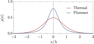
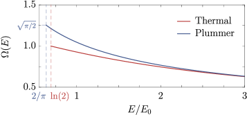
Figure 1: Top: Density profiles of the thermal and Plummer equilibria. The Plummer equilibrium has a sharper core. Bottom: Corresponding frequency profiles. The range of available frequencies is wider for the Plummer equilibrium.

While the thermodynamical equilibrium has a strong core and few particles in the tails (only ${\!\sim\!10^{-9}}$ of the total mass outside ${[-10\Lambda,10\Lambda]}$), the Plummer distribution has a sharper core and much wider tails (${\sim\!10^{-3}}$ of the total mass outside ${[-10\Lambda,10\Lambda]}$). In the second panel of Fig. 1, we present the frequency profile of both equilibria. The Plummer denser core widens its frequency profile, allowing in turn for more resonances. At high energies, both frequency profiles decrease like $1/\sqrt{E}$.

III Long-term Evolution

The long-term relaxation of self-gravitating systems driven by finite-$N$ fluctuations is generically governed by the inhomogeneous BL equation (Heyvaerts, 2010; Chavanis, 2012)

$$\frac{\partial F(J,t)}{\partial t}\!=\!-2\pi^{2}\,m\,\frac{\partial}{\partial J}\!\bigg{[}\sum_{k,k^{\prime}}k\!\!\int\!\!\mathrm{d}J^{\prime}\big{|}\psi^{\mathrm{d}}_{kk^{\prime}}\big{(}J,J^{\prime},k\,\Omega(J)\big{)}\big{|}^{2}$$

$$\times{} \delta_{\mathrm{D}}\big{(}k\,\Omega(J)\!-\!k^{\prime}\,\Omega(J^{\prime})\big{)}\bigg{(}\!k^{\prime}\frac{\partial}{\partial J^{\prime}}\!-\!k\frac{\partial}{\partial J}\!\bigg{)}F(J)\,F(J^{\prime})\bigg{]}.$$ (7)

This non-linear equation describes the long-term evolution of the mean orbital distribution, ${F(J,t)}$, driven by resonant couplings between gravitationally dressed Poisson fluctuations (${m\!\propto\!1/N}$). The sum, ${\sum_{k,k^{\prime}}}$, and integral, ${\!\int\!\mathrm{d}J^{\prime}}$, in Eq. (7) correspond to a scan over the discrete resonances and orbital space. Any time the resonance condition, ${k\,\Omega(J)\!-\!k^{\prime}\,\Omega(J^{\prime})\!=\!0}$, is met, the diffusion is sourced. The system’s propensity to amplify fluctuations is captured in the dressed susceptibility coefficients, ${|\psi^{\mathrm{d}}_{kk^{\prime}}(J,J^{\prime},k\,\Omega)|^{2}}$. Those are the (squared norm of the) Fourier transform (FT) of the pairwise interaction potential dressed by the system’s gravitational susceptibility (see Appendix A.3). In the following, we investigate both cases where the gravitational dressing is (BL) and is not (Landau) taken into account.

III.1 Orbital Diffusion

The BL Eq. (7) can be re-written as a more compact continuity equation in action space

$$\frac{\partial F}{\partial t} =-\frac{\partial\mathcal{F}}{\partial J}$$ (8a)

$$=-\frac{\partial}{\partial J}\left[A(J)F(J)-\tfrac{1}{2}\,D(J)\frac{\partial F}{\partial J}\right],$$ (8b)

with the total flux ${\mathcal{F}(J,t)}$, and the diffusion coefficient

$$D(J)=(2\pi)^{2}m{} \sum_{k,k^{\prime}}k^{2}\!\!\int\!\!\mathrm{d}J^{\prime}\,\big{|}\psi^{\mathrm{d}}_{kk^{\prime}}\big{(}J,J^{\prime},k\,\Omega(J)\big{)}\big{|}^{2}$$

$$\times\delta_{\mathrm{D}}\big{(}k\,\Omega(J)\!-\!k^{\prime}\,\Omega(J^{\prime})\big{)}\,F(J^{\prime}).$$ (9)

In Eq. (8b), the polarization friction, ${A(J)}$, is obtained from Eq. (9) via the substitutions ${(2\pi)^{2}\!\to\!2\pi^{2}}$, ${k^{2}\!\to\!k\,k^{\prime}}$ and ${F\!\to\!\partial F/\partial J^{\prime}}$. As discussed in Sec. 7.4.2 of Binney and Tremaine (2008), the diffusion coefficient also has the simple interpretation

$$D(J)=\underset{T\to+\infty}{\lim}\frac{\left\langle\Delta J^{2}(T)\right\rangle}{T},$$ (10)

with ${\Delta J(T)\!=\!J(t\!=\!T)\!-\!J(t\!=\!0)}$ the change in action of a given particle, and ${\langle\cdot\rangle}$ the ensemble average over realisations. Equations (9) and (10) provide us with two independent means of measuring and predicting ${D(J)}$. In the following, we will focus our interest on the diffusion coefficients in energy, which naturally read ${D_{EE}\!=\!\Omega^{2}D}$.

III.2 Diffusion coefficients

In the top panel of Fig. 2, we present the diffusion coefficients at thermal equilibrium computed with the BL and the Landau formalism, together with the corresponding estimates from numerical simulations.

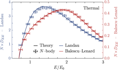
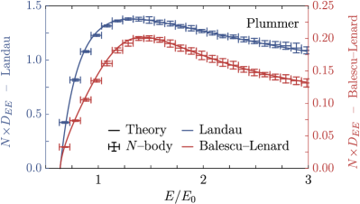
Figure 2: Top: Diffusion coefficients at thermal equilibrium as a function of energy in both Landau (i.e. without collective effects) and BL (i.e. with collective effects) cases. Bottom: Same as the top panel but for the Plummer equilibrium. The kinetic theory shows a very satisfactory match to the numerical measurements. For illustration, both measurements have their own adapted scale as collective effects slow down diffusion by a factor ${\sim\!10}$. See Appendix B.2 for the numerical details.

We refer to Appendix A for the details of the kinetic estimation, and Appendix B for the $N$-body measurements. In both Landau and BL cases, we recover a very good match between the kinetic theory and the numerical measurements. This confirms that, indeed, long-range resonant couplings are responsible for the long-term relaxation of these systems. We stress that the BL diffusion coefficients are ${\sim\!10}$ times smaller than the Landau ones, an effect already noted in the HMF model for highly magnetized thermal equilibria (see fig. 9 in Benetti and Marcos, 2017). This is at variance with the low magnetization HMF result, or the case of self-gravitating stellar disks Fouvry et al. (2015) where collective effects considerably accelerate the relaxation.

In the bottom panel of Fig. 2, we present the same measurements for the Plummer distribution. Satisfactorily, this other equilibrium shows the same level of fine agreement. Similarly, we also find that collective effects slow down the diffusion by a factor ${\sim\!10}$. This will be discussed in Sec. IV.

III.3 Fluxes

We now turn our interest to the initial diffusion flux, ${\mathcal{F}(J,t\!=\!0)}$, as given by Eq. (8). Of course, this flux vanishes for the thermodynamical equilibrium. In Fig. 3, we illustrate the initial diffusion flux for a fully self-gravitating Plummer equilibrium.

Figure 3: Initial flux in the Plummer equilibrium as a function of energy predicted by kinetic theory (line) and measured in $N$-body simulations (points). Both capture the maximum near ${E/E_{0}\!\simeq\!1.25}$, and the change of sign at ${E/E_{0}\!\simeq\!2.5}$. We stress that the amplitude of ${N\!\times\!\mathcal{F}(E)}$ has been rescaled by $10^{5}$. See Appendix B.3 for the numerical details.

Once again, the kinetic theory and numerical simulations are found to be in a good match, and both recover the (slow) relaxation of the Plummer distribution towards the thermal one. Within the appropriate dimensionless units, we point out that the diffusion flux is typically ${\sim\!10^{5}}$ times smaller than the diffusion coefficients, i.e. the efficiency of the relaxation is drastically hampered by a near kinetic blocking. This is further discussed in Sec. IV.1.

III.4 Correlation of the perturbations

Following Fouvry and Bar-Or (2018), we present in Fig. 4 the correlation ${C(t)\!=\!\langle\delta\psi(0)\,\delta\psi(t)\rangle}$ of the potential fluctuations, ${\delta\psi(t)}$, in the $N$-body simulations, as a function ${t/t_{\mathrm{dyn}}}$, with ${t_{\mathrm{dyn}}\!=\!\Lambda/\sigma}$, the dynamical time. This correlation sources orbital diffusion (Binney and Lacey, 1988). We refer to Appendix B.4 for a precise definition of ${C(t)}$.

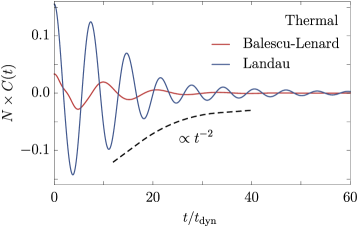
Figure 4: Time correlation, ${C(t)\!=\!\langle\delta\psi(0)\,\delta\psi(t)\rangle}$ of the potential fluctuations in $N$-body simulations of the thermal equilibrium with and without collective effects, as a function of the time ${t/t_{\mathrm{dyn}}}$. See Appendix B.4 for precise definitions. In the presence of collective effects, both the amplitude and coherence time of the correlation fonction are reduced.

The gravitational dressing has two main effects: (i) it weakens the overall amplitude of the potential fluctuations; (ii) it reduces the coherence time of these perturbations. Naturally, this drives a slower orbital diffusion in the BL situation compared to the Landau one, as presented in Sec. III.1.

This is fully consistent with Fig. 5 where we equivalently illustrate the diffusion of individual test particles in the presence/absence of collective effects.

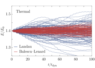
Figure 5: Typical diffusion of test particles embedded within $N$-body realizations of the thermal equilibrium with collective effects (BL) or without (Landau). The massless test particles are all placed at the same initial phase space location in their respective realizations. Collective effects slow down the orbital diffusion.

In that figure, we also recover that the energy diffusion is naturally modulated at the frequency ${\sim 2\pi/t_{\mathrm{dyn}}}$, i.e. the typical frequency of the background thermal equilibrium.

IV Discussion

We now discuss our two main findings: non-thermal equilibria present very inefficient relaxation; and collective effects reduce the efficiency of diffusion.

IV.1 Quasi kinetic blocking

In Fig. 3, we noted that, within appropriate dimensionless units, the diffusion flux in the Plummer equilibrium is ${\sim\!10^{5}}$ times smaller than the associated diffusion coefficients (see Fig. 2). This is the imprint of a (quasi-) kinetic blocking, highlighting the system’s difficulty to populate resonances driving an efficient diffusion.

As put forward in Eq. (7), the system’s long-term diffusion is sourced by resonant interactions. For a given resonant pair ${(k,k^{\prime})}$, one has to ensure that the resonance condition, ${k\Omega(J)\!-\!k^{\prime}\Omega(J^{\prime})\!=\!0}$, is met, while the overall efficiency of this coupling is governed by the susceptibility coefficients, ${\psi_{kk^{\prime}}^{\mathrm{d}}(J,J^{\prime},\omega)}$, for that pair. In practice, a couple of important “conspiracies”, responsible for the small flux observed in Fig. 3, operate:

1. The Plummer frequency profile is monotonic (see Fig. 1). Any resonance ${k\!=\!k^{\prime}}$ systematically imposes ${J\!=\!J^{\prime}}$, leading to an exactly vanishing flux in Eq. (7).

2. Symmetry imposes ${\psi_{kk^{\prime}}^{\mathrm{d}}\!=\!0}$, for all ${k,k^{\prime}}$ of different parity (see Appendix A.4). As a consequence, one must have ${|k\!-\!k^{\prime}|\!\geq\!2}$ for a resonance to contribute to the flux. Similarly, ${k,k^{\prime}}$ must also have the same sign.

3. Despite its denser core, the overall frequency range of the Plummer profile is still finite (see Fig. 1). For a given orbit $J$, this imposes ${k/k^{\prime}\leq\Omega(J\!=\!0)/\Omega(J)}$ for the resonance condition from Eq. (7) to be met.

4. For $k$ large enough, the bare susceptibility coefficients asymptotically scale like ${\psi_{kk}(J,J)\!\propto\!1/k^{2}}$ (see Appendix A.4). The higher order the resonance, the less efficient the coupling, and hence the (drastically) smaller the contribution to the flux.

We highlight these different effects in Fig. 6, where we isolate the contributions, $\mathcal{F}_{kk^{\prime}}$, of the different resonances ${(k,k^{\prime})}$ to the Landau flux ${\mathcal{F}\!=\!\sum_{k,k^{\prime}>0}\mathcal{F}_{kk^{\prime}}}$. We emphasize in particular the rapid decay of the flux contributions as ${k,k^{\prime}}$ increase and as one moves away from the diagonal ${k\!=\!k^{\prime}}$ (which only contributes to the diffusion coefficient and not the flux). These different effects are jointly responsible for the small flux reported in Fig. 3.

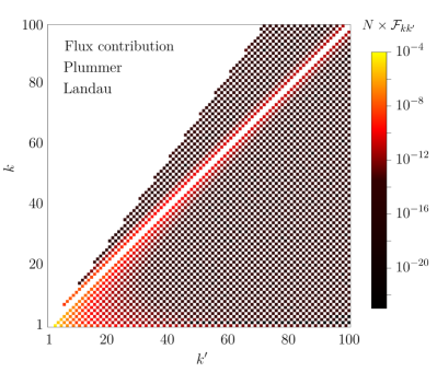
Figure 6: Individual contributions of the various resonances ${(k,k^{\prime})}$ to the initial Landau flux, ${\mathcal{F}(E,t\!=\!0)}$, for the Plummer equilibrium and ${E\!=\!\psi(2\alpha)}$. By symmetry, we only consider ${k,k^{\prime}\!\geq\!0}$ resonances. Note the logarithmic colour coding. The flux is dominated by low order resonances and suffers from many annihilating conspiracies (see main text).

Figure 6 is essentially left unchanged when taking into account collective effects. The only significant difference in the BL case is the reduced contribution from the resonances with ${k\!=\!1}$ for which gravitational dressing weakens the amplitude of the orbital coupling as detailed in Sec. IV.2 and  IV.3. Taking collective effects into account therefore further reduces the flux as they notably damp contribution from the resonance ${(k,k^{\prime})\!=\!(1,3)}$, the main contributor to the Landau flux (see Fig. 6).

Despite this relative inefficiency, we stress that the Plummer equilibrium still relaxes through ${1/N}$ two-body resonant effects. This is in stark contrast with homogeneous ${1D}$ systems which are generically kinetically blocked at order ${1/N}$ (see, e.g., Chavanis, 2012) and require the derivation of appropriate kinetic equations at order ${1/N^{2}}$ sourced by three-body effects (Fouvry et al., 2020).

IV.2 Linear Response

We now discuss the influence of collective effects. The efficiency of the gravitational dressing of perturbations is generically captured by the response matrix, ${\mathbf{M}(\omega)}$ (see, e.g., Eq. (5.94) in Binney and Tremaine, 2008) which reads here

$$\mathbf{M}_{pq}(\omega)=2\pi\sum_{k\in\mathbb{Z}}\!\int\!\mathrm{d}J\,\frac{k\,\partial F/\partial J}{\omega\!-\!k\,\Omega(J)}\,\psi^{(p)*}_{k}\!(J)\,\psi^{(q)}_{k}(J),$$ (11)

with ${\psi^{(p)}_{k}(J)}$ the FT of the bi-orthogonal basis elements. As detailed in Appendix A.2, we construct natural basis elements by periodizing the interaction potential on a ad hoc length $L$. Such a modification impacts the system only on large separations (i.e. small frequencies), which we alleviate by picking $L$ sufficiently large given the system’s density. We refer to Appendix A.5 for details on the computation of the response matrix, in particular regarding the resonant denominator from Eq. (11).

In Fig. 7, we illustrate the determinant of the susceptibility matrix ${[\mathbf{I}-\mathbf{M}(\omega)]^{-1}}$ for the thermal equilibrium, as a function of ${\omega/\Omega_{0}}$, with ${\Omega_{0}\!=\!\sqrt{GM_{\mathrm{tot}}/\Lambda}}$ the (maximum) orbital frequency in the system’s center (${\Omega_{0}\!=\!\sqrt{GM_{\mathrm{tot}}/\alpha}}$ for the Plummer equilibrium).

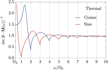
Figure 7: Determinant of the susceptibility matrix, ${[\mathbf{I}\!-\!\mathbf{M}(\omega)]^{-1}}$, as a function of the real frequency ${\omega/\Omega_{0}}$ for the even (cosine) and odd (sine) basis elements (see Appendix A.2). Here, $\Omega_{0}$ is the maximum frequency in the system’s center, while ${\Omega_{L}\!\simeq\!0.35\,\Omega_{0}}$ is the smallest frequency captured by the $L$-periodized potential (${L\!=\!10\,\Lambda}$). Collective effects become negligible at small separation (high frequencies). Conversely, they induce a striking damping for frequencies ${\omega\!\sim\!\Omega_{0}}$, which explains the particular inefficiency of the BL diffusion compared to the Landau one.

Because the system possesses a finite maximum frequency, $\Omega_{0}$, its linear response shows clear signatures at every (resonant) multiple of this frequency. Nonetheless, we find that the collective amplification remains limited, while the same result also holds for the Plummer equilibrium. Conversely, collective effects significantly damp the contribution of the odd resonances ${k\Omega\!\sim\!\Omega_{0}}$, i.e. the lowest order resonances in the most populated regions. These resonances being dominant contributors to the diffusion (see Sec. IV.3), it explains the relative inefficiency of the BL diffusion unveiled in Fig. 2. This is in sharp constrast with ${\ell\!=\!1}$ perturbations in globular clusters (see, e.g., fig. 1 in Fouvry and Prunet, 2022).

IV.3 Impact of collective effects

The influence of the gravitational dressing strongly depends on the resonance frequency, ${\omega\!=\!k\Omega}$. It is therefore of interest to pinpoint the individual contributions of resonances to the diffusion coefficient, ${D\!=\!\sum_{k,k^{\prime}>0}D_{kk^{\prime}}}$.

As for the flux, the allowed resonances must satisfy a parity criterium as well as ${k/k^{\prime}\leq\Omega(J\!=\!0)/\Omega(J)}$, but, however, ${k\!=\!k^{\prime}}$ resonances contribute to the diffusion. Given that the coupling efficiency rapidly drops with the order of the resonance, in Fig. 8, we focus on the contributions of low-order resonances.

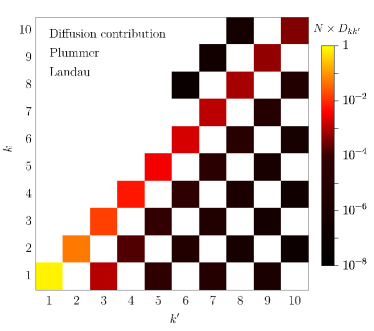
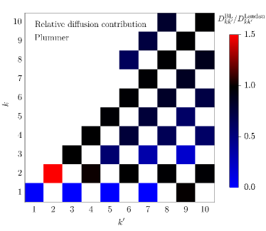
Figure 8: Top: Individual contributions of the various resonances ${(k,k^{\prime})}$ to the Landau diffusion coefficients for the Plummer equilibrium and ${E\!=\!\psi(2\alpha)}$. Bottom: Relative contributions when collective are or not taken into account, for the same setup. The main contributor to the Landau diffusion, resonance ${(1,1)}$, is severely damped by collective effects, while the amplification of other resonances remains limited.

The top panel of this figure illustrates the predominant role of the resonance ${(k,k^{\prime})\!=\!(1,1)}$ in the Landau orbital diffusion (in yellow), while the bottom panel shows the extinguishing role of collective effects for any ${k\!=\!1}$ resonances. This is ultimately responsible for the relative inefficiency of the BL diffusion w.r.t. the Landau one. The determinant of the susceptibility matrix plotted in Fig. 7 allows us to reach the same conclusions. Indeed, the gravitational susceptibility suffers from a drought for any odd resonant couplings with ${\omega\!\sim\!\Omega_{0}}$. And, the slight amplification of the resonance ${(2,2)}$ observed in Fig. 8 is equivalently found in Fig. 7 since ${2\Omega(2\alpha)\!\sim\!1.4\Omega_{0}}$. This amplification remains still too limited to compensate for the strong collective damping of the dominating ${(1,1)}$ resonance.

V Conclusions

The long-term relaxation of discrete self-gravitating systems is driven by the subtle combined effects of finite-${N}$ Poisson fluctuations and long-range orbital resonances, possibly boosted or damped by gravitational polarization. This is captured by the inhomogeneous BL equation (Heyvaerts, 2010; Chavanis, 2012). In this work, we compared its kinetic predictions with $N$-body simulations of ${1D}$ self-gravitating systems.

We focused on the thermal and Plummer equilibria, while accounting and not accounting for collective effects. We reach clear agreement for both models on the rate of diffusion. The BL diffusion coefficients were found to be ${\sim\!10}$ times smaller than the Landau ones, i.e. collective effects surprisingly mitigates diffusion, and we provided an explanation for it. This conclusion is particularly interesting as it is also present in the HMF model in highly magnetized equilibria (Benetti and Marcos, 2017) while it is absent in weakly magnetized ones or in the periodic stellar cube (Magorrian, 2021). This may or may not be the case in higher dimensions (see, e.g., Weinberg, 1989; Fouvry et al., 2015, 2021) possibly depending on the position and geometry of the wake and on these systems’ reservoirs of free energy via rotation or anisotropy.

Similarly, the predicted flux closely matches the measured one for the Plummer equilibrium. This is a remarkable validation of kinetic theory, which was not granted a priori since the BL theory makes strong assumptions about the amplitude of the fluctuations and timescale decoupling between the linear and long-term processes. We discussed how diffusion is mostly driven by low order resonances which can be significantly altered by collective effects. We explained how the vanishing contribution of ${k\!=\!k^{\prime}}$ resonances to the flux leads to a quasi-kinetic blocking, drastically slowing down the relaxation of non-thermal equilibria.

Beyond this work, one should aim at better understanding the precise origin of the ability of collective effects to accelerate/slow down relaxation. For example, one could investigate sets of equilibria closer to marginal stability, e.g., with bumps on tail, and identify the possible importance of their damped modes (see, e.g., Weinberg, 1994). In the spirit of the low magnetization HMF model (Benetti and Marcos, 2017), one may expect that collective modes would ultimately boost the BL flux over the Landau one.

Given the accuracy achieved for the initial flux, it would clearly be useful to integrate Eq. (7) self-consistently in time. This is no easy undertaking, as it involves tracking both the non-linear dependence in $F$ and the joint evolution of the mean potential and the associated angle-action coordinates (see, e.g., Weinberg, 2001). This same ${1D}$ model may also prove useful to understand the relaxation of thickened galaxies (see, e.g., Fouvry et al., 2017). More generally, it bodes well for future implementations in higher dimensions, as in globular clusters, or dark matter halos.

Appendix A ${1D}$ kinetic theory

A.1 Angle-action coordinates

Following Eq. (3.195) of Binney and Tremaine (2008), the action of an orbit is the circulation of ${v}$ for one full radial oscillation. For an even mean-field potential ${\psi(r\!=\!|x|)}$, it simply reads

$$J=\frac{1}{\pi}\!\!\int_{-r_{\mathrm{a}}}^{r_{\mathrm{a}}}\!\!\mathrm{d}x\,v=\frac{2\,\sqrt{2}}{\pi}\!\!\int_{0}^{r_{\mathrm{a}}}\!\!\mathrm{d}r\,\sqrt{\psi(r_{\mathrm{a}})-\psi(r)},$$ (12)

with $r_{\mathrm{a}}$ the orbit’s apocenter, i.e. the maximum radius reached during the particle’s libration which satisfies ${E\!=\!\psi(r_{\mathrm{a}})}$. In the following sections, we equivalently use $r_{\mathrm{a}}$, $E$ and $J$ to label orbits. The orbital frequency, ${\Omega\!=\!\partial H/\partial J}$, and the associated angle $\theta$, satisfying $\dot{\theta}=\Omega$, read

$$\frac{1}{\Omega} =\frac{\sqrt{2}}{\pi}\int_{0}^{r_{\mathrm{a}}}\!\!\frac{\mathrm{d}x}{\sqrt{\psi(r_{\mathrm{a}})-\psi(x)}},$$ (13a)

$$\theta(x,r_{\mathrm{a}}) =\frac{\Omega(r_{\mathrm{a}})}{\sqrt{2}}\int_{\mathcal{C}}\frac{\mathrm{d}x^{\prime}}{\sqrt{\psi(r_{\mathrm{a}})-\psi(x^{\prime})}},$$ (13b)

with ${\mathcal{C}}$ the contour going from ${x\!=\!-r_{\mathrm{a}}}$ up to the current position ${x\!=\!x(\theta)}$ along the radial oscillation. Therefore, the angle mapping is such that

$$x(\theta\!=\!0)=-r_{\mathrm{a}};\;x(\tfrac{\pi}{2})=0;\;x(\pi)=r_{\mathrm{a}};\;x(\tfrac{3\pi}{2})=0.$$ (14)

To cure the divergence of the integrand of Eq. (13) for ${x\!\rightarrow\!\pm r_{\mathrm{a}}}$, we perform the change of variables ${x\!=\!r_{\mathrm{a}}f(u)}$ towards an effective anomaly ${-1\!\leq\!u\!\leq\!1}$ satisfying ${f(\pm)\!=\!1}$ and ${f^{\prime}(\pm 1)\!=\!0}$. This change of variable must be: (i) explicit (no inversion needed), (ii) stable (to sample numerous nearby points), (iii) generic (must work for any analytic potential). In practice, we use the polynomial anomaly ${f(u)\!=\!u(\tfrac{3}{2}\!-\!\tfrac{1}{2}u^{2})}$ Hénon (1971).

To address the arising ${0/0}$ limit in the integrand

$$I(u,r_{\mathrm{a}})=\frac{r_{\mathrm{a}}f^{\prime}(u)}{\sqrt{\psi(r_{\mathrm{a}})-\psi(r_{\mathrm{a}}f(u))}},$$ (15)

we use a second-order Taylor expansion in ${u\!\to\!\pm 1}$ and ${r_{\mathrm{a}}/\Lambda\!\to\!0^{+}}$, as soon as ${|1\!\pm\!u|\!\leq\!10^{-3}}$ or ${r_{\mathrm{a}}/\Lambda\!\leq\!10^{-3}}$. Benefiting from this numerically stable approach, the integrals from Eqs. (12) and (13) are computed using Simpson’s ${1/3}$-rule, with $100$ uniforms intervals in ${u\in[0,1]}$.

A.2 Biorthogonal basis

Following Kalnajs (1976), the bi-orthogonal basis elements satisfy

$$\psi^{(p)}(x)=\!\!\int\!\!\mathrm{d}x^{\prime}\,\rho^{(p)}(x^{\prime})\,U(x,x^{\prime}),{}$$ (16a)

$$\!\!\int\!\!\mathrm{d}x\,\rho^{(p)}(x)\,\psi^{(q)*}(x)=-\delta_{pq}.{}$$ (16b)

With them, the pairwise interaction potential becomes

$$U(x,x^{\prime})=-\sum_{p}\psi^{(p)}(x)\,\psi^{(p)*}(x^{\prime}).$$ (17)

To construct basis elements, we periodize ${U(x,x^{\prime})}$ on a period ${2L}$, so that it becomes $U_{\mathrm{per}}(x,x^{\prime})\!=\!U(x,x^{\prime})$ for ${|x\!-\!x^{\prime}|\leq L}$, and $U_{\mathrm{per}}(x\!+\!2kL,x^{\prime})\!=\!U_{\mathrm{per}}(x,x^{\prime})$ for ${k\!\in\!\mathbb{Z}}$. Dropping the constant term, the periodized potential, $U_{\mathrm{per}}$, is decomposed in Fourier series via

$$U_{\mathrm{per}}{} (x,x^{\prime})=-\frac{4GL}{\pi^{2}}\sum\limits_{\begin{subarray}{c}p\textrm{ odd}\\ p>0\end{subarray}}\frac{1}{p^{2}}$$ (18)

$$\times{} \big{[}\cos\big{(}p\tfrac{\pi}{L}x\big{)}\cos\big{(}p\tfrac{\pi}{L}x^{\prime}\big{)}+\sin\big{(}p\tfrac{\pi}{L}x\big{)}\sin\big{(}p\tfrac{\pi}{L}x^{\prime}\big{)}\big{]}.$$

Following Eq. (17), the natural basis elements are then

$$\psi^{(p)}_{\mathrm{even}}(x)=\frac{2\sqrt{GL}}{p\,\pi}\cos\big{[}p\tfrac{\pi}{L}x\big{]},$$ (19)

with ${p\!>\!0}$ odd, and their odd counterpart $\psi^{(p)}_{\mathrm{odd}}$ via ${\cos\!\to\!\sin}$. Following Eq. (2), the associated densities are

$$\rho^{(p)}_{\mathrm{even}}(x)=\frac{-\pi^{2}\,p^{2}}{2GL^{2}}\psi^{(p)}_{\mathrm{even}}(x),$$ (20)

and equivalently for the odd ones. It is straightforward to check that Eqs. (19) and (20) comply with Eq. (16) for the periodized potential, $U_{\mathrm{per}}$, when restricting the integration range to ${-L\!\leq\!x\!\leq\!L}$.

In practice, the basis elements are computed from coupled recurrence relations (see Eq. (5.4.6) in Press et al., 2007). In the main text, we use a periodization length $L\!=\!10\Lambda$ (resp. $L\!=\!100\Lambda$) and 256 (resp. 1024) basis elements for thermal (resp. Plummer) computations. Indeed, since the Plummer equilibrium density has wide tails (see Fig. 1), a large $L$ is required which, in turn, requires more basis elements to reach a sufficient resolution.

A.3 Fourier transform in angles

Once a suitable bi-orthogonal basis has been constructed, one has to compute the FT of the basis element, ${\psi_{k}^{(p)}(J)}$, involved in both the response matrix from Eq. (11) and the dressed coupling coefficient

$$\psi^{\mathrm{d}}_{kk^{\prime}}(J,J^{\prime},\omega)=-\sum_{p,q}\psi_{k}^{(p)}(J)\,\big{[}\mathbf{I}\!-\!\mathbf{M}(\omega)\big{]}^{-1}_{pq}(\omega)\,\psi^{(q)*}_{k^{\prime}}(J^{\prime}),$$ (21)

with $\mathbf{I}$ the identity matrix, and ${\mathbf{M}(\omega)}$ the system’s response matrix (Eq. 11). Given the convention from Eq. (14), the FT of the basis elements reads

$$\psi_{k}^{(p)}(J)=\frac{1}{\pi}\!\!\int_{0}^{\pi}\!\!\mathrm{d}\theta\,\psi^{(p)}\big{(}x[\theta,J]\big{)}\cos(k\theta).$$ (22)

To compute this integral, we naturally perform the same change of variables as in Appendix A.1. One is left with two integrals that must be performed simultaneously

$$\psi^{(p)}_{k}(J) =\frac{1}{\pi}\int_{-1}^{1}\!\!\mathrm{d}u\,\frac{\mathrm{d}\theta}{\mathrm{d}u}\,\psi^{(p)}(x[u])\,\cos(k\,\theta[u]),$$ (23a)

$$\theta[u] =\!\!\int_{-1}^{u}\!\!\mathrm{d}u^{\prime}\,\frac{\mathrm{d}\theta}{\mathrm{d}u^{\prime}},$$ (23b)

where ${\mathrm{d}\theta/\mathrm{d}u\!=\!\Omega(r_{\mathrm{a}})I(u,r_{\mathrm{a}})/\sqrt{2}}$ with ${I(u,r_{\mathrm{a}})}$ defined in Eq. (15). Although the integrals from Eqs. (23) seem nested, they can be evaluated via the single integral of a $2$-vector (Rozier et al., 2019). In practice, we use a fourth-order Runge-Kutta (RK4) scheme with $10^{3}$ steps for ${u\in[-1,1]}$.

A.4 Bare coupling coefficients

In the Landau case, collective effects can be neglected. As such, in Eq. (21), one makes the replacement ${[\mathbf{I}-\mathbf{M}(\omega)]^{-1}\!\to\!\mathbf{I}}$, and the dressed coupling coefficients, ${\psi_{kk^{\prime}}^{\mathrm{d}}(J,J^{\prime},\omega)}$ become the bare ones, ${\psi_{kk^{\prime}}(J,J^{\prime})}$. Importantly, these coefficients can be computed without any basis expansion, as they are the Fourier transform of the pairwise interaction w.r.t. the angle $\theta$ (Chavanis, 2013). Using the effective anomaly ${u}$ from Appendix A.1, the frequency-independent bare coupling coefficients become

$$\psi_{kk^{\prime}}(J,J^{\prime})=\frac{1}{\pi^{2}}\!\!\int_{-1}^{1}\!\!\mathrm{d}u\,\mathrm{d}u^{\prime}\;g(x)\,g^{\prime}(x^{\prime})\;U(x,x^{\prime}),$$ (24)

with ${g(x)\!=\!\cos(k\theta)\,\mathrm{d}\theta/\mathrm{d}u}$ (and similarly for $g^{\prime}$). Symmetry imposes ${\psi_{kk^{\prime}}(J,J^{\prime})\!=\!0}$ for any $k,k^{\prime}$ of different parity. The same result also holds for the dressed susceptibility coefficients, ${\psi_{kk^{\prime}}^{\mathrm{d}}(J,J^{\prime},\omega)}$, from Eq. (21).

To compute Eq. (24), each anomaly, $u,u^{\prime}$, is sampled with $K$ nodes at the location ${u_{i}\!=\!-1\!+\!2(i\!-\!\tfrac{1}{2})/K}$ with ${1\!\leq\!i\!\leq\!K}$. Equation (24) becomes

$$\psi_{kk^{\prime}}(J,J^{\prime})=\frac{4G}{\pi^{2}K^{2}}\sum_{i,j=1}^{K}g_{i}\,g^{\prime}_{j}\,|x_{i}-x^{\prime}_{j}|,$$ (25)

where the ${g_{i}\!=\!g(x_{i})\!=\!g(x(u_{i}))}$ (and ${g^{\prime}_{j}}$) are pre-computed in a single pass using a direct integration of ${\mathrm{d}\theta/\mathrm{d}u}$, following Eq. (23), requiring $\mathcal{O}(K)$ operations.

The quasi-separable form of the pairwise interaction potential allows us to rewrite Eq. (25) as

$$\psi_{kk^{\prime}}(J,J^{\prime})=\frac{4G}{\pi^{2}K^{2}}\sum_{j=1}^{K}g^{\prime}_{j}\,\big{(}P_{j}+Q_{j}\big{)},$$ (26)

with the cumulative sums

$$P_{j}=\sum_{i=1}^{w_{j}}g_{i}\,\big{(}x^{\prime}_{j}-x_{i}\big{)},\;Q_{j}=\sum_{\mathclap{i=w_{j}+1}}^{K}g_{i}\,\big{(}x_{i}-x^{\prime}_{j}\big{)},$$ (27)

and ${w_{j}\!=\!\mathrm{Card}\big{\{}i\in\llbracket 1,K\rrbracket\,\big{|}\,x_{i}\leq x^{\prime}_{j}\big{\}}}$. Importantly, $P_{j}$ and $Q_{j}$ can both be computed in a single pass, requiring overall ${\mathcal{O}(K)}$ operations to estimate ${\psi_{kk^{\prime}}(J,J^{\prime})}$. In practice, we used ${K\!=\!10^{3}}$ nodes, and an RK4 scheme to compute ${g_{i},g^{\prime}_{j}}$. We note that for ${k\!\gg\!1}$, ${\psi_{kk}(J,J)\!\propto\!1/k^{2}}$, which explains the minor role played by high order resonances, as in Fig. 6.

A.5 Computing the response matrix

The response matrix from Eq. (11) involves a sum over the resonances ${k}$, and an integral over the action ${J}$ with a resonant denominator. This asks for a careful treatment.

Benefiting from the rapid decay of the coupling coefficients, we can safely truncate the sum over $k$ to ${|k|\!\leq\!k_{\mathrm{max}}}$. In practice, ${k_{\mathrm{max}}\!=\!10}$ proves highly sufficient.

To deal with the resonant integral from Eq. (11), we follow the approach from Fouvry and Prunet (2022):

1. The truncated action domain $[J_{0},J_{L}]$ (with ${J_{0}\!=\!J(r_{\mathrm{a}}\!=\!0)}$ and ${J_{L}\!=\!J(r_{\mathrm{a}}\!=\!L)}$) is remapped to ${[-1,1]}$ via ${y=\mathrm{Sign}(k)(\Omega(J)\!-\!\Sigma_{\Omega})/\Delta_{\Omega}}$ with ${\Sigma_{\Omega}\!=\!\tfrac{1}{2}(\Omega_{0}\!+\!\Omega_{L})}$, ${\Delta_{\Omega}\!=\!\tfrac{1}{2}(\Omega_{0}\!-\!\Omega_{L})}$, ${\Omega_{0}\!=\!\Omega(J_{0})}$ and ${\Omega_{L}\!=\!\Omega(J_{L})}$. Equation (11) then becomes

   $$M_{k}^{pq}(\omega)=\!\!\int_{-1}^{1}\!\!\mathrm{d}y\,\frac{G_{k}^{pq}(y)}{y-\varpi_{k}},$$ (28)

   with

   $$G_{k}^{pq}(y) =2\pi\,\mathrm{Sign}(k)\,\frac{\mathrm{d}J}{\mathrm{d}\Omega}\frac{\partial F}{\partial J}\psi_{k}^{(p)*}(J)\,\psi_{k}^{(q)}(J),$$ (29a)

   $$\varpi_{k} =\frac{\omega}{|k|\Delta_{\Omega}}-\mathrm{Sign}(k)\frac{\Sigma_{\Omega}}{\Delta_{\Omega}},$$ (29b)

   where $J$ depends implicitly on $y$.

2. The numerator ${G_{k}^{pq}(y)}$ in Eq. (29a) is projected onto Legendre polynomials via ${G_{k}^{pq}(y)\!=\!\sum_{\ell=0}^{\ell_{\mathrm{max}}}a_{k\ell}^{pq}\,P_{\ell}(y)}$, using a Gauss-Legendre (GL) quadrature truncated to $\ell_{\mathrm{max}}$ (${=\!100}$ in practice). Equation (28) then becomes $M_{k}^{pq}(\omega)=\sum_{\ell=0}^{\ell_{\mathrm{max}}}a_{k\ell}^{pq}\,D_{k\ell}(\omega)$ with

   $$D_{k\ell}(\omega)=\!\!\int_{-1}^{1}\!\!\mathrm{d}y\frac{P_{\ell}(y)}{y-\varpi_{k}}.$$ (30)

3. We apply Landau’s prescription (see, e.g., Sec. 5.2.4 in Binney and Tremaine, 2008) to compute ${D_{k0}}$ and ${D_{k1}}$, while $D_{k\ell}$ for ${\ell\geq 2}$ are computed via direct recurrences (see Appendix D in Fouvry and Prunet, 2022).

A.6 Quasi-stationary states

The equilibrium DFs presented in Sec. II.2 are obtained by Eddington inversion (see, e.g., Sec. 4.3.1 in Binney and Tremaine, 2008). For a symmetric density profile, the density ${\rho(r\!=\!|x|)\!=\!2\!\int\!_{0}^{+\infty}\!\mathrm{d}v\,F(E)}$, can be expressed as

$$\rho(\psi)=\sqrt{2}\!\!\int_{\psi}^{+\infty}\!\!\!\!\mathrm{d}E\frac{F(E)}{\sqrt{E-\psi}},$$ (31)

with $\psi=\psi(r)$. Following Eq. (B.72) of Binney and Tremaine (2008), this Abel integral equation is inverted as

$$F(E)=\frac{\sqrt{2}}{\pi}\!\!\int_{E}^{+\infty}\!\!\!\!\mathrm{d}\psi\sqrt{\psi-E}\,\frac{\mathrm{d}^{2}\rho}{\mathrm{d}\psi^{2}}.$$ (32)

Finally, using the relation ${\psi(x)\!=\!\int\!\mathrm{d}x^{\prime}\rho(x^{\prime})U(x,x^{\prime})}$, one readily finds the potential of the thermal equilibrium

$$\psi(x)=GM_{\mathrm{tot}}\Lambda\log\left[2\cosh\left(x/\Lambda\right)\right],$$ (33)

as well for the Plummer quasi-stationnary equilibrium

$$\psi(x)=GM_{\mathrm{tot}}\alpha\,\sqrt{1+(x/\alpha)^{2}}.$$ (34)

The DF from Eq. (4) is the usual Boltzmann distribution $F(E)\propto e^{-mE/k_{\mathrm{B}}T}$ of statistical mechanics with the specific energy $E$, and a thermodynamical temperature ${k_{\mathrm{B}}T\!=\!mE_{0}/2}$. Using the virial theorem, one can relate the total energy $E_{\rm tot}$ to the temperature $T$, characteristic velocity $\sigma$ and characteristic length $\Lambda$ by ${E_{\mathrm{tot}}\!=\!\tfrac{3}{2}Nk_{\mathrm{B}}T\!=\!\tfrac{3}{4}M_{\mathrm{tot}}\sigma^{2}\!=\!\tfrac{3}{4}GM_{\mathrm{tot}}^{2}\Lambda}$.

Figure 9 illustrates typical mean-fields orbit in the thermal and Plummer equilibria. Both display similar phase space diagrams, although Plummer’s orbits reach larger central velocity owing to their denser core (Fig. 1).

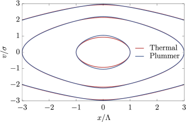
Figure 9: Typical mean-field (closed) orbits in phase-space, for apocenters ${r_{\mathrm{a}}/\Lambda\!=\!(1,3,5)}$. Because the Plummer equilibrium is more peaked than the thermal one, its orbits reach a larger maximal velocity in the system’s center.

Appendix B $N$-body integration

B.1 Method

The system’s total Hamiltonian is

$$H_{\mathrm{tot}}=\sum_{i=1}^{N}\tfrac{1}{2}m_{i}v_{i}^{2}+\sum_{i<j}m_{i}m_{j}\,U(x_{i},x_{j}),$$ (35)

so that the equations of motion for particle ${i}$ read

$$\dot{x}_{i}{}=v_{i};\quad\dot{v}_{i}{}=G\left(M^{\mathrm{r}}_{i}-M^{\mathrm{l}}_{i}\right),$$ (36)

with ${M^{\mathrm{r}}_{i}}$ (resp. ${M^{\mathrm{l}}_{i}}$) the total mass on the right (resp. on the left) of particle ${i}$. Importantly, by sorting the set ${\{x_{i}\}}$, one can compute these cumulative masses in a single pass. Determining the (exact) instantaneous forces on all particles requires therefore ${\mathcal{O}(N\ln(N))}$ operations.

The present ${1D}$ system can be integrated exactly using a collision-driven scheme (Noullez et al., 2003). However, this approach requires ${\mathcal{O}(N^{2}\ln(N))}$ operations per dynamical time, making long-time integrations of large-$N$ systems too challenging. As such, we rather settle on using an approximate time integrator (with exact forces). Because Eq. (35) is separable, one can use standard splitting methods (see, e.g., Hairer et al., 2006) to devise integration schemes. The main source of error comes from the abrupt force changes every time particles cross, making it wiser to limit oneself to low-order schemes. We use the standard leapfrog scheme (see, e.g., Sec. 3.4.1 in Binney and Tremaine, 2008) which requires a single (costly) force evaluation per timestep, ${\delta t}$, and an overall $\mathcal{O}(N\ln(N)\,t_{\mathrm{dyn}}/\delta t)$ operations per dynamical time.

In Fig. 10, we check the sanity of our algorithm, by illustrating the conservation of the total energy, $E_{\mathrm{tot}}$, as one varies the timestep ${\delta t}$, the number of particles, $N$, and the overall number of integration time steps, ${t/\delta t}$.

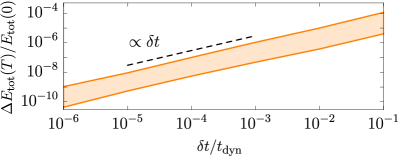
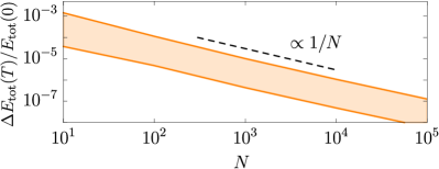
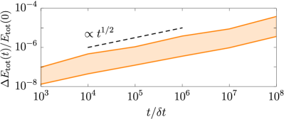
Figure 10: Relative error in the system’s total energy, $E_{\mathrm{tot}}$, as a function of (i) the timestep ${\delta t}$ (with ${N\!=\!10^{4}}$, ${T/t_{\mathrm{dyn}}\!=\!100}$), (ii) the number of particles $N$ (with ${\delta t/t_{\mathrm{dyn}}\!=\!10^{-3}}$, ${T/t_{\mathrm{dyn}}\!=\!100}$), (iii) the total number of integration steps ${t/\delta t}$ (with ${N\!=\!10^{4}}$, ${\delta t/t_{\mathrm{dyn}}\!=\!10^{-3}}$).

Because the pairwise interaction, ${U(x,x^{\prime})}$, does not have a continuous derivative, the leapfrog scheme is only first-order accurate, i.e. its error scales like ${\mathcal{O}(\delta t)}$ after a fixed finite-time (top panel). As one increases $N$, these discontinuities weaken, so that the error at finite time scales like ${\mathcal{O}(1/N)}$ (center panel). Finally, for the present explicit scheme, we empirically find that the error in $E_{\mathrm{tot}}$ grows like $\sqrt{t}$ as a function of time (bottom panel).

To prevent the $N$-body realizations from drifting away, we systematically perform the operation ${v_{i}\!\leftarrow\!v_{i}\!-\!\sum_{i=1}^{N}\!m_{i}v_{i}/M_{\mathrm{tot}}}$ at the simulation’s onset, hence setting the system’s total momentum to zero. Such a recentring slightly blurs the effective DF in velocity space (and therefore in energy) by an amount proportional to ${1/\sqrt{N}}$. To mitigate this effect, we always chose values of $N$ large enough, e.g., ${N\!=\!10^{5}}$ as in Fig. 2.

In the Landau simulations, we introduce two types of particles: (i) massive background particles that follow the smooth mean potential, and (ii) massless test particles driven by the instantaneous (noisy) potential generated by the background particles. The orbital diffusion undergone by these test particles corresponds to the (undressed) Landau diffusion.

B.2 Diffusion measurements

To estimate diffusion coefficients in $N$-body simulations, we follow Eq. (10). First, for the sake of convenience, we measure diffusion in energy, ${E\!=\!v^{2}/2\!+\!\psi(x)}$, computed with ${\psi(x)}$ the system’s initial unperturbed potential. For a given realization, particles are initially binned in 25 bins of width ${\delta E_{\mathrm{bin}}\!=\!0.1\,E_{0}}$ starting at the minimal energy ${\psi(0)}$. For every bin and every time dump, we compute ${\langle\Delta E^{2}(t)\rangle\!=\!\langle(E(t)\!-\!E(t\!=\!0))^{2}\rangle}$, averaged over all the particles initially in the bin and all the available realizations. In practice, the associated time series, ${t\!\to\!\langle\Delta E^{2}(t)\rangle}$ is truncated at a time $T_{\mathrm{max}}$ chosen so that ${\langle\Delta E^{2}(T_{\mathrm{max}})\rangle\!\leq\!\delta E_{\mathrm{bin}}^{2}}$. This ensures that particles have not diffused so much as to explore too different energies.

Because the system’s fluctuations are correlated, the series of ${\langle\Delta E^{2}\rangle}$ are not always linear function of time, but exhibit initially a quadratic dependence w.r.t. time. This occurs during the ballistic time, $T_{\mathrm{bal}}$, which, fortunately is independent of $N$ (see Fig. 4). It is important not to perform any measurement within this early phase. A final caveat stems from the fact that at large time, the BL time series become sub-linear, a phenomenon already noted in the HMF model (see Fig. 8 in Benetti and Marcos, 2017). This is accounted for by appropriately reducing the series’ maximal time, $T_{\mathrm{max}}$, so as not to enter this regime.

Once the domain ${T_{\mathrm{bal}}\!\leq\!t\!\leq\!T_{\mathrm{max}}}$ determined, we rely on Eq. (10) and estimate the diffusion coefficient with a linear fit (least squares) on that timespan. This is illustrated in Fig. 11 for both Landau and BL measurements.

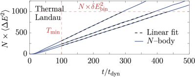
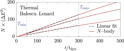
Figure 11: Typical time series of energy dispersion averaged over a given energy bin and ${1\,280}$ realizations for Landau (top panel) and BL measurements (bottom), together with the associated linear fit. Here, ${\langle\Delta E^{2}\rangle}$ first evolves quadratically in time (ballistic regime) and then linearly (diffusive regime). For the BL experiments, the time series ultimately becomes sublinear, as already noted in the HMF model (Benetti and Marcos, 2017).

For the BL measurements in Fig. 2, we ran $10$ independent groups of ${1\,280}$ realizations with ${N\!=\!10^{5}}$ particles, with ${\delta t\!=\!10^{-3}\,t_{\mathrm{dyn}}}$ up to ${T\!=\!500\,t_{\mathrm{dyn}}}$, reaching a typical relative error in $E_{\mathrm{tot}}$ of order $10^{-6}$, and dumping ${\Delta E^{2}}$ values every $t_{\mathrm{dyn}}$. As illustrated in Fig. 11, we performed the linear fit within the domain ${[T_{\mathrm{bal}},T_{\mathrm{max}}]\!=\![50,300]\!\times\!t_{\mathrm{dyn}}}$. In Fig. 2, we report the mean value and standard deviation of the $10$ independent batches of realizations.

For the Landau experiments, we use the exact same parameters, except that the ${N\!=\!10^{5}}$ massive background particles follow the smooth mean potential, and we injected ${2\!\times\!10^{4}}$ massless test particles sampled initially according to ${F(E)}$. Because Landau simulations exhibit longer correlation times (see Fig. 4), we use ${T_{\mathrm{bal}}\!=\!100\,t_{\mathrm{dyn}}}$ and adjusted ${T_{\mathrm{max}}}$ for every bin so that ${\langle\Delta E^{2}(T_{\mathrm{max}})\rangle\!\leq\!\delta E_{\mathrm{bin}}^{2}}$, as illustrated in Fig. 11.

B.3 Flux measurements

To estimate the diffusion flux from Eq. (8), we rely on the easy to measure cumulative density of state (DoS)

$$G(E)=\!\!\int_{-\infty}^{E}\!\!\mathrm{d}E^{\prime}\,P(E^{\prime}),$$ (37)

with ${P(E)\!=\!2\pi F(E)/\Omega(E)}$ the DoS in energy, normalized so that ${\!\int\!\mathrm{d}E\,P(E)\!=\!1}$. Following Eq. (8a), we naturally have ${\mathrm{d}G/\mathrm{d}t\!=\!-2\pi\mathcal{F}(E)}$. Consequently, to measure the flux, we simply count the number of particles with an (unperturbed) energy smaller than a given energy threshold $E$, and keep track of this quantity as a function of time. Once averaged over realizations, the flux, ${\mathcal{F}(E)}$, is directly estimated via linear fits. These measurements are more challenging than that of the diffusion coefficients because the Plummer flux is particularly small (Fig. 3).

In pratice, we ran $10$ independent groups of ${1\,280}$ realizations with ${N\!=\!10^{4}}$ particles, with ${\delta t\!=\!10^{-3}\,t_{\mathrm{dyn}}}$ up to ${T\!=\!10^{4}\,t_{\mathrm{dyn}}}$, reaching a typical relative error on $E_{\mathrm{tot}}$ of order $10^{-5}$, and dumping values of interest every ${10\,t_{\mathrm{dyn}}}$. In Fig. 3, we report the mean value and standard deviations over these $10$ independent batches.

B.4 Correlation measurements

As emphasized in Binney and Lacey (1988), orbital diffusion is generically sourced by the time correlation of the potential fluctuations, which here stem from Poisson shot noise. The instantaneous density ${\rho_{\mathrm{d}}(x,t)\!=\!\sum_{i}m\delta_{\mathrm{D}}(x\!-\!x_{i}(t))}$ can easily be projected onto the biorthogonal basis (Appendix A.2) to write ${\rho_{\mathrm{d}}(x,t)\!=\!\sum_{p}A_{p}(t)\rho^{(p)}(x)}$ with

$$A_{p}(t)=-\sum_{i}m\,\psi^{(p)}(x_{i}(t)).$$ (38)

We use these coefficients to probe the time evolution of the system’s finite-$N$ fluctuations In Fig. 4, we illustrate the correlation

$$C(t)=\!\!\int_{0}^{T-t}\!\!\!\!\frac{\mathrm{d}\tau}{T-t}\langle A_{p}(\tau)A_{p}(\tau+t)\rangle,$$ (39)

for the odd basis element ${\psi_{\mathrm{odd}}^{(3)}}$, following Eq. (19). In practice, we ran ${1\,280}$ realizations of the thermal equilibrium with ${N\!=\!10^{5}}$ particles, with ${\delta t\!=\!10^{-3}\,t_{\mathrm{dyn}}}$ up to ${T\!=\!10^{3}\,t_{\mathrm{dyn}}}$, reaching a typical relative error on $E_{\mathrm{tot}}$ of order $10^{-6}$, and dumping values of ${A_{p}}$ every ${0.05\,t_{\mathrm{dyn}}}$. For the BL experiment, we also let the system “warm up” during $200$ dynamical times before any measurement, so as to let the initial Poisson shot noise thermalize and get dressed by collective effects (see, e.g., Appendix F in Fouvry and Bar-Or, 2018).

References

- Heyvaerts (2010) J. Heyvaerts, MNRAS 407, 355 (2010).
- Chavanis (2012) P.-H. Chavanis, Physica A 391, 3680 (2012).
- Fouvry et al. (2015) J.-B. Fouvry, C. Pichon, J. Magorrian, and P.-H. Chavanis, A&A 584, A129 (2015).
- Fouvry et al. (2021) J.-B. Fouvry, C. Hamilton, S. Rozier, and C. Pichon, MNRAS 508, 2210 (2021).
- Joyce and Worrakitpoonpon (2010) M. Joyce and T. Worrakitpoonpon, J. Stat. Mech. 2010, P10012 (2010).
- Solway et al. (2012) M. Solway, J. A. Sellwood, and R. Schönrich, MNRAS 422, 1363 (2012).
- Bovy et al. (2012) J. Bovy et al., ApJ 753, 148 (2012).
- Zel’dovich (1970) Y. B. Zel’dovich, A&A 5, 84 (1970).
- Valageas (2006) P. Valageas, Phys. Rev. E 74, 016606 (2006).
- Benetti and Marcos (2017) F. P. C. Benetti and B. Marcos, Phys. Rev. E 95, 022111 (2017).
- Lynden-Bell (1967) D. Lynden-Bell, MNRAS 136, 101 (1967).
- Spitzer (1942) J. Spitzer, Lyman, ApJ 95, 329 (1942).
- Camm (1950) G. L. Camm, MNRAS 110, 305 (1950).
- Rybicki (1971) G. B. Rybicki, Astrophys. Space Sci. 14, 56 (1971).
- Eddington (1916) A. S. Eddington, MNRAS 76, 572 (1916).
- Hénon (1973) M. Hénon, A&A 24, 229 (1973).
- Horedt (2004) G. P. Horedt, Polytropes (Kluwer Acad. Publ., 2004).
- Binney and Tremaine (2008) J. Binney and S. Tremaine, Galactic Dynamics: Second Edition (Princeton Univ. Press, 2008).
- Fouvry and Bar-Or (2018) J.-B. Fouvry and B. Bar-Or, MNRAS 481, 4566 (2018).
- Binney and Lacey (1988) J. Binney and C. Lacey, MNRAS 230, 597 (1988).
- Fouvry et al. (2020) J.-B. Fouvry, P.-H. Chavanis, and C. Pichon, Phys. Rev. E 102, 052110 (2020).
- Fouvry and Prunet (2022) J.-B. Fouvry and S. Prunet, MNRAS 509, 2443 (2022).
- Magorrian (2021) J. Magorrian, MNRAS 507, 4840 (2021).
- Weinberg (1989) M. D. Weinberg, MNRAS 239, 549 (1989).
- Weinberg (1994) M. D. Weinberg, ApJ 421, 481 (1994).
- Weinberg (2001) M. D. Weinberg, MNRAS 328, 321 (2001).
- Fouvry et al. (2017) J.-B. Fouvry, C. Pichon, P.-H. Chavanis, and L. Monk, MNRAS 471, 2642 (2017).
- Hénon (1971) M. Hénon, Astrophys. Space Sci. 13, 284 (1971).
- Kalnajs (1976) A. J. Kalnajs, Astrophys. J. 205, 745 (1976).
- Press et al. (2007) W. Press et al., Numerical Recipes 3rd Edition (Cambridge Univ. Press, 2007).
- Rozier et al. (2019) S. Rozier et al., MNRAS 487, 711 (2019).
- Chavanis (2013) P.-H. Chavanis, A&A 556, A93 (2013).
- Noullez et al. (2003) A. Noullez, D. Fanelli, and E. Aurell, J. Comput. Phys. 186, 697 (2003).
- Hairer et al. (2006) E. Hairer, C. Lubich, and G. Wanner, Geometric numerical integration: Second Edition (Springer, 2006).