Gaussian matrix product states cannot efficiently describe critical systems

Abstract

Gaussian fermionic matrix product states (GfMPS) form a class of ansatz quantum states for 1d systems of noninteracting fermions. We show, for a simple critical model of free hopping fermions, that: (i) any GfMPS approximation to its ground state must have bond dimension scaling superpolynomially with the system size, whereas (ii) there exists a non-Gaussian fermionic MPS approximation to this state with polynomial bond dimension. This proves that, in general, imposing Gaussianity at the level of the tensor network may significantly alter its capability to efficiently approximate critical Gaussian states. We also provide numerical evidence that the required bond dimension is subexponential, and thus can still be simulated with moderate resources.

The growing complexity of quantum many-body wavefunctions with increasing system sizes has motivated the development of variational classes of states. By exploiting simplifying features of a given problem, ansatz states can help optimize numerical resources, as well as provide an insightful new perspective into the inner workings of quantum correlations in these systems. For instance, Gaussian states and their correlation matrix formalism greatly facilitate computations involving non-interacting particles. On the other hand, tensor network states have become an essential theoretical framework and numerical toolbox for quantum many-body physics, excelling at the representation of area law and similarly low-entangled states Cirac21 .

For systems of free (or weakly interacting) fermions, both classes can be combined to give rise to Gaussian fermionic tensor network states Kraus10 . Relevant examples include the ground state of the Kitaev-Majorana chain, and models of topological insulators and superconductors Wahl13 ; Dubail15 ; Wahl14 ; Yang15 . In the 1d case, the resulting tensor network is the Gaussian fermionic matrix product state or GfMPS, which has been shown to outperform non-tensor network based methods in free fermion computations for very large systems Schuch19 . This motivates the question about the expressivity of GfMPS, namely what kind of free fermionic states can be efficiently described by them.

In the case of general MPS, it was proved in Verstraete06 that an efficient approximation (i.e. one with bond dimension growing at most polynomially with the system size $N$) exists whenever a certain Rényi entropy is bounded by $O(\log N)$. This established the usefulness of MPS to approximate states with at most a logarithmic violation of the area law, including the ground states of both gapped and gapless (critical) local Hamiltonians. In the setting of fermionic chains, it also applies to fermionic MPS (fMPS). However, it is not known whether an analogous result holds for GfMPS whenever the state being approximated is Gaussian with similarly bounded entropies.

Here we answer this question in the negative: we provide a simple counterexample in the form of a critical hopping fermion Hamiltonian, whose Gaussian ground state can be efficiently approximated by fMPS but not by GfMPS. The proof of this last fact combines a rigorous bound on the error incurred by a fixed rank Gaussian approximation of a Gaussian state with specific knowledge of the entanglement structure of the target ground state, obtained from asymptotic Toeplitz determinant theory. Furthermore, we provide evidence, both from conformal field theory arguments and numerical results, that the required bond dimension scaling for a good GfMPS approximation is nevertheless subexponential. This makes the question about the existence of an efficient GfMPS approximation a hard one to settle numerically, which motivated our pursuit of an analytical proof.

Our result disproves the somewhat intuitive assumption that the most bond dimension-efficient approximation to a Gaussian state would come from a Gaussian tensor network. This can be relevant when optimizing resources for computational applications, though it should be noted that the savings due to having access to the correlation matrix formalism may well compensate the extra bond dimension derived from Gaussianity. Additionally, there are other situations where Gaussian tensor networks have faced difficulty approximating Gaussian states, as is the case for ground states of local, gapped, quadratic Hamiltonians displaying chiral topological features Wahl13 ; Dubail15 . In this context, our findings leave the door open to the existence of better, non-Gaussian tensor network approximations that bypass the no-go results.

Model— We consider a periodic chain of length $N$ with a single fermionic mode $a_{i},a_{i}^{\dagger}$ per site, satisfying the usual canonical anticommutation relations,

$$\{a^{\phantom{\dagger}}_{i},a^{\dagger}_{j}\}=\delta_{ij},\qquad\{a_{i},a_{j}\}=\{a^{\dagger}_{i},a^{\dagger}_{j}\}=0,$$ (1)

and study the free hopping Hamiltonian at half filling,

$$H=-\dfrac{1}{2}\sum_{j=1}^{N}{a^{\dagger}_{j}a^{\phantom{\dagger}}_{j+1}}+\text{h.c.}=-\sum_{k}{\cos{k}~{}a^{\dagger}_{k}a^{\phantom{\dagger}}_{k}},$$ (2)

where we have defined the momentum modes in the usual form, ${a_{k}\equiv\frac{1}{\sqrt{N}}\sum_{j=1}^{N}{e^{ikj}a_{j}}}$ with $k\in\frac{2\pi}{N}\mathbb{Z}\cap(-\pi,\pi]$. In this basis $H$ is diagonal and its ground state, which is Gaussian due to $H$ being quadratic, can be determined by filling the negative energy modes below the Fermi momentum, $k_{F}=\pi/2$ . This is encoded in the momentum space correlation matrix,

$$C_{kq}\equiv\langle a^{\dagger}_{k}a^{\phantom{\dagger}}_{q}\rangle=n_{k}\delta_{k,q},\qquad n_{k}\equiv\Theta(k_{F}-|k|),$$ (3)

where $\Theta$ denotes the Heaviside step function. The position space correlation matrix $C_{ij}\equiv\langle a^{\dagger}_{i}a^{\phantom{\dagger}}_{j}\rangle$ can then be obtained by an inverse Fourier transform. It exhibits power-law decays as befits a gapless model (its explicit form can be seen in Appendix C). Note that due to particle number conservation, $\langle a_{k}a_{q}\rangle=\langle a_{i}a_{j}\rangle=0$.

The entanglement structure of this state, which will be key to the results presented next, can be obtained from its correlation matrix. Given a bipartition of a pure Gaussian state into complementary regions $\mathcal{R},\bar{\mathcal{R}}$, we can find a basis of modes on each subsystem such that the state decomposes as the tensor product of entangled fermion pairs Botero04 . How entangled these pairs are is given by the spectrum of the correlation matrix of either subsystem, which is nothing but the corresponding submatrix of the global correlation matrix,

$$C_{\mathcal{R}}\equiv(C_{ij})_{i,j\in\mathcal{R}}.$$ (4)

For convenience and notational unity we will work with the eigenvalues of $V_{\mathcal{R}}\equiv 2C_{\mathcal{R}}-\mathds{1}$, which we denote ${\{\lambda_{j}\}\subset[-1,1]}$, and call the Gaussian entanglement spectrum . The Rényi entropy $S_{\alpha}$ then splits as a sum of contributions from each entangled pair,

$$S_{\alpha}=\sum_{j}{s_{\alpha}(\lambda_{j})},$$ (5)

where

$$s_{\alpha}(\lambda)\equiv\dfrac{1}{1-\alpha}\log\left[\left(\dfrac{1+\lambda}{2}\right)^{\alpha}+\left(\dfrac{1-\lambda}{2}\right)^{\alpha}\right],$$ (6)

so that the entanglement decreases with $|\lambda|$ from $\lambda=0$ (maximally entangled state) to $\lambda=\pm 1$ (product state).

For the ground state of $H$, the leading scaling of the Rényi entropy of an interval of size $L$ can be seen to be logarithmic Vidal03 ; Jin04 ; Peschel09 ,

$$S_{\alpha}(L)\sim\dfrac{\alpha+1}{6\alpha}\log L,\qquad L\to\infty,$$ (7)

which is consistent with it lying in the universality class of the free boson conformal field theory (CFT) with central charge $c=1$ Holzhey94 ; Calabrese04 .

Efficient approximation with fMPS — A fermionic matrix product state (fMPS) Kraus10 is defined in terms of a series of so-called fiducial states of $f$ physical fermions and $2\chi$ virtual fermions. The state represented by the fMPS is obtained by contracting the virtual fermions, i.e. projecting them onto maximally entangled pairs (see Fig. 1). The dimension $D$ of the virtual Hilbert space, i.e. the bond dimension (b.d.) of the fMPS, is related to $\chi$ via $D=2^{\chi}$ .

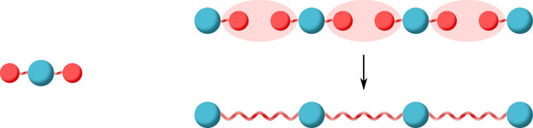
Figure 1: (left) A (G)fMPS fiducial state of one physical fermion and two virtual fermions. (right) A (G)fMPS is obtained from projecting the virtual fermions onto entangled pairs, leaving an entangled state of the physical fermions.

Definition 1.

A family of states $|\Psi_{N}\rangle$ for increasing system sizes $N$ is efficiently approximable by fMPS if for any $\epsilon>0$ there exists a family of fMPS states $|\Psi^{\text{\tiny MPS}}_{N}\rangle$ with b.d. $D(N)=\text{\emph{poly}}(N)$ and

$$\||\Psi_{N}\rangle-|\Psi^{\text{\tiny MPS}}_{N}\rangle\|_{2}\leq\epsilon\quad\forall N.$$ (8)

Theorem 1.

The family of ground states of (2) is efficiently approximable by fMPS.

Proof.

Using the Jordan-Wigner transformation, we can map our system to a spin chain model, the XX model. Since we have a logarithmic bound (7) for the Rényi entropies, in particular for $\alpha<1$, it follows from Lemmas 1 and 2 in Verstraete06 that the ground state of the XX model is efficiently approximable by MPS. Then, undoing the Jordan-Wigner transformation, we can find an efficient fMPS approximation for the fermionic model (this is done in detail in Appendix A). ∎

In general, understanding the entanglement structure of quantum states is key to obtain both approximability and inapproximability results, since the bond dimension of an MPS has a clear interpretation as the maximum Schmidt rank for a bipartition of an MPS into connected subsystems. In order to compare it with an analogous result in the next section, we cite here the following

Lemma 1 (Low Schmidt rank approximation).

Let $|\Psi\rangle$ by a bipartite quantum state with Schmidt spectrum $\{s_{j}\}_{j=1}^{n}$ in descending order. Then for any bipartite state $|\tilde{\Psi}\rangle$ of Schmidt rank at most $r$,

$$|\langle\Psi|\tilde{\Psi}\rangle|^{2}\leq 1-\sum_{j=r+1}^{n}{s_{j}^{2}},$$ (9)

and the bound is tight: the optimal $|\tilde{\Psi}\rangle$ can be found by truncating the Schmidt decomposition of $|\Psi\rangle$.

Lemma 1 is a consequence of the Eckart-Young-Mirsky theorem Eckart36 ; Mirsky60 , which states that the optimal low rank approximation to a given matrix comes from truncating its singular value decomposition. It leads to a lower bound for the error of an MPS approximation (used for instance in some of the inapproximability proofs in Schuch08 ).

No efficient approximation with Gaussian fMPS — A Gaussian fMPS (GfMPS) is an fMPS for which all fiducial states are Gaussian. Since the contraction operation projects each pair of virtual modes onto a Gaussian state, the maximally entangled pair, the global state after contraction is necessarily Gaussian. The contraction of GfMPS tensors can be done at the level of correlation matrices via Schur complements Bravyi05 ; Schuch19 (see Appendix D).

An efficient approximation in terms of GfMPS can be defined analogously to the fMPS case. Then, we have our main result as

Theorem 2.

The family of ground states of (2) is not efficiently approximable by GfMPS.

The proof of Theorem 2 will follow from two lemmas. The first one is the Gaussian version of Lemma 1. Given the Gaussian entanglement spectrum $\{\lambda_{j}\}$ of a bipartite state, we call the number of eigenvalues $\lambda_{j}\neq\pm 1$ its Gaussian rank. We then have

Lemma 2 (Low Gaussian rank approximation).

Let $|\Psi\rangle$ be a bipartite Gaussian state, with Gaussian entanglement spectrum $\{\lambda_{i}\}_{i=1}^{n}$, ordered so that $|\lambda_{i}|\leq|\lambda_{i+1}|$. Then for any Gaussian state $|\tilde{\Psi}\rangle$ of Gaussian rank at most $r$,

$$|\langle\Psi|\tilde{\Psi}\rangle|^{2}\leq\prod_{i=r+1}^{n}{\dfrac{1+|\lambda_{i}|}{2}}=\exp{\left(-S_{\infty}^{\emph{trunc}}[r]\right)},$$ (10)

where $S_{\infty}^{\emph{trunc}}[r]\equiv\sum_{i=r+1}^{n}{s_{\infty}(\lambda_{i})}$, and the bond is tight: the optimal $|\tilde{\Psi}\rangle$ can be found by truncating the Gaussian singular value decomposition of $|\Psi\rangle$.

We were not able to find a proof in the literature so we provide one together with related results in Appendix B. Lemma 2 can be used to lower bound the error of a GfMPS approximation to a given state, since the Gaussian rank of any GfMPS divided into two connected subsystems is upper bounded by $\chi$. We then need information on the entanglement spectrum of our target state, which is provided by

Lemma 3.

For the ground state of (2), let $\mathcal{I}_{L,N}(\mu)$ be the number of eigenvalues $\lambda$ from the Gaussian entanglement spectrum of an interval of size $L$ in a chain of $N$ sites that satisfy $|\lambda|<\mu$, and let $c>0$. Then there exists $\mu<1$ such that

$$\mathcal{I}_{L,N}(\mu)>c\log N,$$ (11)

as $L,N\to\infty$ with $L/N$ fixed.

The proof of Lemma 3 can be found in Appendix C. It starts by proving the equivalent property for the Gaussian entanglement spectra of the infinite chain: in the thermodynamic limit, we can exploit the theory of Toeplitz determinants to lower bound the corresponding $\mathcal{I}_{L,\infty}(\mu)$ function in the asymptotic regime. Then we use standard inequalities to show that the difference between the finite and infinite chain correlation matrices is bounded in trace norm. This ensures that their respective spectra are distributed similarly enough so that Lemma 3 follows.

Proof (of Thm. 2).

Suppose there exists a GfMPS approximation with polynomial b.d. $D(N)$. Then we can find ${c>0}$ such that ${\chi(N)=\log_{2}{D(N)}\leq c\log N}$. Thanks to Lemma 3, we know there exists some ${\mu<1}$ such that ${\mathcal{I}_{L,N}(\mu)>(c+1)\log N}$, and we have

$$S_{\infty}^{\emph{trunc}}[\chi(N)] \geq(\mathcal{I}_{L,N}(\mu)-\chi(N))s_{\infty}(\mu)$$

$$\geq s_{\infty}(\mu)\log N,$$ (12)

which diverges as $N\to\infty$. Since $|\tilde{\Psi}_{N}\rangle$ has Gaussian rank bounded by $\chi(N)$ across the bipartition, Lemma 2 implies that the overlap between the ground state and its GfMPS approximation goes to zero as the system size increases. Thus, by contradicion, any approximation with bounded error must have $\chi(N)$ growing faster than logarithmically, and consequently $D(N)$ grows superpolynomially. ∎

CFT argument — The techniques used in the proof of Theorem 2 cannot be applied to obtain better lower bounds, or upper bounds on the required b.d., for which more accurate knowledge of the Gaussian entanglement spectra of finite chains would be needed. Here we provide evidence that this b.d. is subexponential. First, a heuristic argument is made, based on conformal field theory (CFT). In the next section, we present some numerical results.

The low-lying entanglement spectrum of a critical model is know to behave universally according to the underlying CFT. With our notation, for an interval of $L$ sites in an chain of $N$ sites, we have Peschel04 ; Lauchli13 ; Ohmori15 ; Cardy16

$$|\lambda_{n}|\simeq\tanh{\left(\dfrac{\pi^{2}}{2}\dfrac{\varepsilon_{n}}{\log\ell}\right)},\qquad\ell=\dfrac{N}{\pi a}\sin{\dfrac{\pi L}{N}}$$ (13)

where $\ell$ is the effective length of our interval in units of some UV cutoff $a$, and the $\varepsilon_{n}$ are fixed by the CFT. In our model, this is the free compactified boson CFT, and

$$\varepsilon_{n}\equiv\left\lfloor\dfrac{n}{2}\right\rfloor+\dfrac{1}{2}=\dfrac{1}{2},\dfrac{1}{2},\dfrac{3}{2},\dfrac{3}{2},\dfrac{5}{2},\dfrac{5}{2}\ldots$$ (14)

(More precisely, these numbers characterize the spectrum of scaling dimensions of an associated boundary CFT.) The CFT spectrum (13) not only satisfies the condition in Lemma 3, but it also allows us to estimate the tail contribution to the $\infty$-Rényi entropy,

$$S_{\infty}^{\text{trunc}}[\chi]\approx\dfrac{2\log\ell}{\pi^{2}}\exp\left(-\dfrac{\pi^{2}\chi}{2\log\ell}\right).$$ (15)

Thus, if the CFT prediction were exact for the whole spectrum, by Lemma 2 the required scaling for $\chi$ is

$$\chi(N,\epsilon)\approx\dfrac{2}{\pi^{2}}\log{\eta N}\log\left(\dfrac{\pi^{2}}{2\epsilon}\log{\eta N}\right),$$ (16)

for some proportionality constant $\ell=\eta N$. Here we used the fidelity error $\epsilon\equiv 1-\exp{\left(-S_{\infty}^{\emph{trunc}}[\chi]\right)}$ attached to a single bipartition of the system. Our experience from MPS is that we should account for all bipartitions, with different $L/N$ and thus different $\eta$ Verstraete06 . We do this coarsely by replacing $\epsilon\to\epsilon/N$. This results in

$$D(N,\epsilon)\approx(\eta N)^{\frac{\log 2}{\pi^{2}}\log{\left(\frac{2N\log\eta N}{\pi^{2}\epsilon}\right)}},$$ (17)

which is subexponential.

Numerics — We have also performed some numerical studies of this problem which seem to partially confirm the scaling from (16). We introduce them briefly here, and elaborate on them in Appendix D. Essentially, we defined a subclass of translation invariant GfMPS (which we call ladder GfMPS), which exactly represent states with the following occupation number in momentum space:

$$n_{k}=\dfrac{p(\cos\frac{k}{2})^{2}}{p(\cos\frac{k}{2})^{2}+q(\sin\frac{k}{2})^{2}},$$ (18)

for $p,q$ arbitrary real odd monic polynomials. Clearly, to reproduce (3), we need to have $p$ (resp. $q$) supported mostly inside (resp. outside) the Fermi surface. We tried several choices, the best of which is represented in Fig. 2. There we have used $\delta\equiv\langle\Psi^{\text{\tiny MPS}}|H_{\text{fb}}|\Psi^{\text{\tiny MPS}}\rangle-E_{0}$, with $H_{\text{fb}}$ the flat band Hamiltonian with the same ground state as $H$, and $E_{0}$ its ground state energy, as a proxy for the fidelity error $\epsilon$, which it upper bounds. Further energy optimization (as done in Mortier20 ), which we did not pursue, could improve the results. Fig. 2 also shows the estimation (17) for $\eta\sim 1.3$ (resulting from optimization), which gives an idea of the scaling of our numerical results.

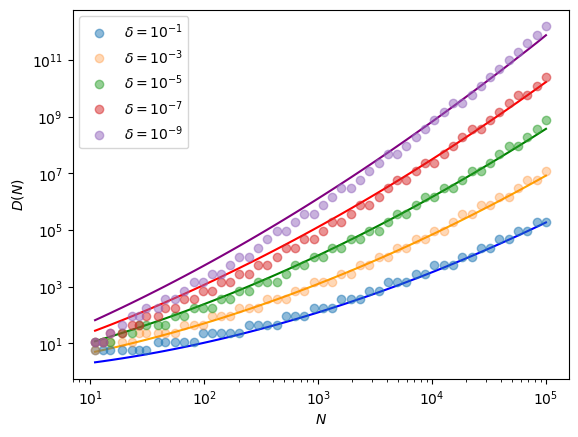
Figure 2: Bond dimension $D(N)$ vs. system size $N$ for our (not necessarily optimal) ladder GfMPS approximation to the ground state of $H$. $\delta$ is the error in energy, which upper bounds the fidelity error $\epsilon$. The lines represent (17) with numerically optimized $\eta\sim 1.3$.

Toy model — Finally, we present a simple toy model of a family of Gaussian states, with no reference to a Hamiltonian, that are efficiently approximable by fMPS but not by GfMPS. We begin by explaining the intuition behind it. Lemmas 1 and 2 highlight the differences between Gaussian and non-Gaussian truncation of a bipartite state . This dichotomy is also reflected in different bounds for the truncation errors, $\epsilon_{G}$ and $\epsilon_{NG}$ resp., in terms of the $\alpha<1$ Rényi entropy. Assuming $\epsilon_{G},\epsilon_{NG}\ll 1$, we have,

$$\epsilon_{G} \lesssim S_{\alpha}^{1/\alpha}\chi^{-(1-\alpha)/\alpha},$$ (19)

$$\epsilon_{NG} \lesssim S_{\alpha}^{1/\alpha}D^{-(1-\alpha)/\alpha}.$$ (20)

For the non-Gaussian case this is Lemma 2 in Verstraete06 . The Gaussian case can be proved similarly by minimizing the entropy over all possible Gaussian entanglement spectra with a fixed Gaussian truncation error. Since $\chi\sim\log D$, we see that the bond for $\epsilon_{G}$ is much weaker, i.e. there exist states with small $S_{\alpha}$ and $\epsilon_{NG}$ but high $\epsilon_{G}$ for the same bond dimension . These states are usually characterized by Gaussian entanglement spectra involving many low-entangled pairs.

We exploit this in our toy example, leveraging the addition of entangled pairs as we grow the system by making their entanglement increasingly weaker. Consider a family of states $|\psi_{N}\rangle$ on rings of $N$ sites obtained by distributing $\nu(N)$ entangled pairs between opposite sites in the chain, each with strength $\lambda_{N}$, where

$$\nu(N)\sim(\log N)^{1+\beta},\quad\lambda_{N}\sim 1-\dfrac{2}{\nu(N)},$$ (21)

for some $\beta>0$. The $\alpha<1$ Rényi entropy is maximal for a bipartition of the ring into two equal halves, since all pairs contribute to give

$$S_{\alpha}(N/2) =\nu(N)s_{\alpha}(\lambda_{N})\sim(\log N)^{(1-\alpha)(1+\beta)},$$ (22)

which is upper bounded by $O(\log N)$ for $\alpha\in\left(\frac{\beta}{1+\beta},1\right)$. Therefore, for any $\beta>0$ an efficient fMPS approximation exists. However, for any GfMPS approximation $|\tilde{\psi}_{N}\rangle$, the error bound (10) reads

$$|\langle\psi_{N}|\tilde{\psi}_{N}\rangle| \leq\left(\dfrac{1+\lambda_{N}}{2}\right)^{\nu(N)-\chi(N)}$$ (23)

$$\lesssim\left(1-\dfrac{1}{\nu(N)}\right)^{\nu(N)-\chi(N)}.$$ (24)

Thus if $|\langle\psi_{N}|\tilde{\psi}_{N}\rangle|\geq 1-\epsilon$, then for large enough $N$ and small enough $\epsilon$ we have

$$\chi(N)\gtrsim\left(1-\epsilon\right)\nu(N)\sim(\log N)^{1+\beta},$$ (25)

so that $D(N)\gtrsim N^{(\log N)^{\beta}}$. This scaling can be easily seen to be sufficient (since $\chi(N)=\nu(N)$ allows for an exact representation), so that the required b.d. to approximate $|\psi_{N}\rangle$ is superpolynomial but still subexponential.

Acknowledgments — A.F.R. would like to thank F. Ares for introducing him to Toeplitz asymptotics a few years ago. A.F.R. is supported by the Alexander von Humboldt Foundation. I.C. acknowledges funding from the ERC Grant QUENOCOBA (No 742102) and the DFG through the DACH Lead Agency Agreement Beyond C (No 414325145).

Appendix A fMPS approximations from (spin) MPS approximations

Following Kraus10 , a fermionic MPS with $f=1$ physical fermions and $2\chi=2$ virtual fermions per site can be defined by means of a series of “projectors”

$$Q_{j}\equiv\sum_{\begin{subarray}{c}k,l,m~{}=~{}0,1\\ k\oplus l\oplus m=p\end{subarray}}{[A_{j}]^{k}_{lm}~{}(a^{\dagger}_{j})^{k}~{}\alpha_{j}^{l}~{}\beta_{j}^{m}},$$ (26)

where $\oplus$ denotes the sum in $\mathbb{Z}_{2}$, $j$ is the position index along the chain, $[A_{j}]^{k}_{lm}$ is a coefficient tensor, and $a_{j},\alpha_{j},\beta_{j}$ are the physical, left virtual and right virtual fermionic modes at site $j$, respectively. The restriction on the indices ensures a well-defined fermionic parity $p$ for $Q_{j}$. One also needs to define the operators

$$H_{j}=\dfrac{1}{\sqrt{2}}\left(\mathds{1}+\beta^{\dagger}_{j}\alpha^{\dagger}_{j+1}\right),$$ (27)

which generate entangled pairs of virtual fermions from the vacuum. The fMPS state is then defined by the action of both sets of operators on the global vacuum, followed by projecting out the virtual fermions:

$$|\Psi\rangle\equiv\langle 0|_{\text{virtual}}\prod_{j}{Q_{j}}\prod_{j}{H_{j}}|0\rangle_{\text{all}}.$$ (28)

The generalization to larger physical and/or bond dimensions is straightforward. If we now interpret the fermionic Fock space as the Hilbert space of a spin $\frac{1}{2}$ chain (as is done implicitly by the Jordan-Wigner transformation), one can see that $|\Psi\rangle$ can be obtained from a standard “spin” MPS, with local tensors that coincide with $[A_{j}]^{k}_{lm}$, possibly up to signs. Consequently, the set of 1d fMPS states coincides with those obtained from MPS that satisfy: (i) their bond dimension is a power of 2, and (ii) each tensor has a well-defined parity.

In the case we are interested in, the Jordan-Wigner transformation maps the fermionic Hamiltonian $H$ from (2) to the XX model spin chain,

$$H_{XX}=\dfrac{1}{2}\sum_{j}{\left[X_{j}X_{j+1}+Y_{j}Y_{j+1}\right]},$$ (29)

for which the results from Verstraete06 apply, since all its Rényi entropies grow logarithmically (see Eq. (7)). The existence of an MPS approximation with polynomial bond dimension then follows. Additionally, this spin MPS has a global parity symmetry represented by the action of the product of $Z$ operators on each physical spin. To see that this implies the existence of an fMPS approximation to the ground state with polynomial b.d., we show that we can make the spin MPS satisfy conditions (i) and (ii) without a substantial increase in bond dimension.

Let $D$ be the bond dimension of the spin MPS, and $[B_{j}]^{k}_{lm}$ denote its tensors. Then there is $q$ such that $D\leq 2^{q}<2D$, and we can embed the $D\times D\times 2$-dimensional MPS tensors into $2^{q}\times 2^{q}\times 2$-dimensional ones without changing the state just by padding each tensor with zeros, i.e. by extending the range of $l,m$ to $2^{q}$, and defining the additional tensor elements as 0. Thus we can satisfy (i) with less than twice the original bond dimension. To get condition (ii), we modify the tensors by adding an additional pair of indices $l^{\prime},m^{\prime}\in\{0,1\}$ such that

$$[B_{j}]^{k}_{ll^{\prime}mm^{\prime}}\equiv[B_{j}]^{k}_{lm}\delta_{k\oplus|l|\oplus|m|\oplus l^{\prime}\oplus m^{\prime}},$$ (30)

where $|l|,|m|$ denotes the parity of the corresponding index. The new tensors are individually parity symmetric, so that (ii) holds, and they can be seen to generate the same state as the original ones (which is only possible because said state has global parity symmetry). Thus it follows that there exists an fMPS approximation to the ground state of $H$, with less than four times the bond dimension of the spin MPS approximation to the XX model ground state, which therefore grows at most polynomially.

Appendix B Gaussian bipartite state overlaps and Gaussian entanglement spectrum

In this Appendix we prove Lemma 2 as a corollary to a more general result. For convenience, we work here in the Majorana representation, introducing Majorana operators

$$c_{j,1}\equiv a^{\phantom{\dagger}}_{j}+a^{\dagger}_{j},\qquad c_{j,2}\equiv i(a^{\phantom{\dagger}}_{j}-a^{\dagger}_{j}),$$ (31)

$$\{c_{j,s},c_{j^{\prime},s^{\prime}}\}=2\delta_{j,j^{\prime}}\delta_{s,s^{\prime}}$$ (32)

so that the (Majorana) correlation matrix is a real, skew-symmetric matrix defined as

$$[\Gamma]_{js,j^{\prime}s^{\prime}}\equiv\dfrac{i}{2}\langle[c_{j,s},c_{j^{\prime},s^{\prime}}]\rangle\qquad s,s^{\prime}=1,2,$$ (33)

which satisfies $\Gamma\Gamma^{\text{T}}\leq\mathds{1}$, with equality for pure states. The overlap of two Gaussian states of $2N$ Majorana fermions can be computed from their correlation matrices $\Gamma,\gamma$, Bravyi05

$$\left|\langle\Gamma|\gamma\rangle\right|^{2}=2^{-N}\sqrt{\det(\mathds{1}-\Gamma\gamma)}.$$ (34)

Finally, we introduce the Gaussian singular value decomposition (Gaussian SVD) Botero04 , which states that, given $\Gamma$ the correlation matrix of a pure bipartite Gaussian state on two subsystems of $2n$ Majorana fermions each , we can find $O,Q\in O(2n)$ that block diagonalize $\Gamma$,

$$\Gamma=(O\oplus Q)\left(\bigoplus_{j=1}^{n}{W(\theta_{j})}\right)(O\oplus Q)^{\text{T}},$$ (35)

where the $4\times 4$ blocks are given by

$$W(\theta)\equiv\left(\begin{array}[]{cc}\cos\theta J&\sin\theta\mathds{1}\\ -\sin\theta\mathds{1}&-\cos\theta J\end{array}\right),\quad J\equiv\left(\begin{array}[]{cc}0&1\\ -1&0\end{array}\right),$$ (36)

and the $\theta_{j}$ can all be chosen to lie on the first quadrant, $0\leq\theta_{j}\leq\frac{\pi}{2}$, in which case we have $\cos\theta_{j}=|\lambda_{j}|$. The $\theta_{j}$ are another possible way to write the Gaussian entanglement spectrum. Indeed, $W(\theta)$ is the correlation matrix of a pair of fermionic modes, which is in a product state for $\sin{\theta}=0$ ($|\lambda|=1$) and maximally entangled whenever $\cos{\theta}=0$ ($\lambda=0$). The number $r$ of entangled pairs ($\sin{\theta}\neq 0$) is what we called in the main text the Gaussian rank. Now we are ready to state and prove the following

Theorem 3.

Let $|\Gamma\rangle,|\tilde{\Gamma}\rangle$ be pure bipartite Gaussian states on two subsystems of $2n$ Majorana fermions. Let their correlation matrices be $\Gamma,\tilde{\Gamma}$ and their Gaussian entanglement spectra be given by $\{\theta_{j}\}_{j=1}^{n},\{\tilde{\theta}_{j}\}_{j=1}^{n}$ respectively. Then,

$$\left|\langle\Gamma|\tilde{\Gamma}\rangle\right|^{2}\leq\max_{\sigma\in S_{n}}\prod_{i=1}^{n}{\cos^{2}\left(\dfrac{\theta_{i}-\tilde{\theta}_{\sigma(i)}}{2}\right)},$$ (37)

and the bound is tight (it is reached for some $\Gamma,\tilde{\Gamma}$).

Proof.

We follow a strategy inspired by Thm. VI.7.1 in Bhatia96 . $\Gamma,\tilde{\Gamma}$ will be of the form

$$\Gamma=(O\oplus Q)\left(\bigoplus_{j=1}^{n}{W(\theta_{j})}\right)(O\oplus Q)^{\text{T}},$$ (38)

$$\tilde{\Gamma}=(\tilde{O}\oplus\tilde{Q})\left(\bigoplus_{j=1}^{n}{W(\tilde{\theta}_{j})}\right)(\tilde{O}\oplus\tilde{Q})^{\text{T}},$$ (39)

for some $O,\tilde{O},Q,\tilde{Q}\in O(2n)$. To begin with, we shall assume that

$$\theta_{i},\tilde{\theta}_{i}\in\left(0,\frac{\pi}{2}\right),\qquad \forall i,$$ (40)

$$\theta_{i}\neq\theta_{j},\tilde{\theta}_{i}\neq\tilde{\theta}_{j},\qquad i\neq j.$$ (41)

We are seeking to upper bound

$$\left|\langle\Gamma|\tilde{\Gamma}\rangle\right|^{2}=2^{-2n}\sqrt{\det(\mathds{1}-\Gamma\tilde{\Gamma})}=2^{-2n}\sqrt{\det{(\Gamma+\tilde{\Gamma})}},$$ (42)

where we have used (34) and the purity condition ${\Gamma^{-1}=-\Gamma}$. In other words, our problem consists in determining

$$\max_{\begin{subarray}{c}O,Q,\\ \tilde{O},\tilde{Q}\end{subarray}}\det((O\oplus Q)W(O\oplus Q)^{\text{T}}+(\tilde{O}\oplus\tilde{Q})\tilde{W}(\tilde{O}\oplus\tilde{Q})^{\text{T}})$$ (43)

where

$$W\equiv\left(\bigoplus_{j=1}^{n}{W(\theta_{j})}\right),\qquad\tilde{W}\equiv\left(\bigoplus_{j=1}^{n}{W(\tilde{\theta}_{j})}\right),$$ (44)

We know the maximum exists since we are optimizing over a closed manifold. Further, we can assume $O,Q=\mathds{1}$, which amounts to fixing the mode basis on which we express our states and does not affect their overlap.

Assume that $(\Gamma,\tilde{\Gamma})$ constitute an extreme point of the target function. This implies that no infinitesimal change in the matrix $\tilde{\Gamma}$ will change the overlap, that is,

$$\left.\dfrac{d}{dt}\det(\Gamma+e^{t(o\oplus q)}\tilde{\Gamma}e^{-t(o\oplus q)})\right|_{t=0}=0,\quad\forall o,q\in\mathfrak{o}(2n).$$ (45)

By differentiating, and then using $\det(\Gamma+\tilde{\Gamma})>0$ (since we are looking for maxima) and the cyclicity of the trace, we arrive at

$$\det(\Gamma+\tilde{\Gamma})\operatorname{tr}{\left((\Gamma+\tilde{\Gamma})^{-1}[o\oplus q,\tilde{\Gamma}]\right)} =0,$$

$$\operatorname{tr}{\left((o\oplus q),[\tilde{\Gamma},(\Gamma+\tilde{\Gamma})^{-1}]\right)} =0.$$ (46)

Let $[\tilde{\Gamma},(\Gamma+\tilde{\Gamma})^{-1}]$, which is skew-symmetric, have the following block structure (according to the bipartition of our states),

$$[\tilde{\Gamma},(\Gamma+\tilde{\Gamma})^{-1}]\equiv\left(\begin{array}[]{cc}A&B\\ -B^{\text{T}}&D\end{array}\right),$$ (47)

with $A=-A^{\text{T}},D=-D^{\text{T}}$. Then condition (46) implies

$$\operatorname{tr}{\left(\left(\begin{array}[]{cc}o&0\\ 0&q\end{array}\right)\left(\begin{array}[]{cc}A&B\\ -B^{\text{T}}&D\end{array}\right)\right)}=\operatorname{tr}{(oA+qD)}=0,$$ (48)

which holds for every skew-symmetric $o,q$. This forces $A=D=0$ and we conclude

$$[\tilde{\Gamma},(\Gamma+\tilde{\Gamma})^{-1}]=\left(\begin{array}[]{cc}0&B\\ -B^{\text{T}}&0\end{array}\right).$$ (49)

We denote $\mathcal{B}\equiv[\tilde{\Gamma},(\Gamma+\tilde{\Gamma})^{-1}]=-[\Gamma,(\Gamma+\tilde{\Gamma})^{-1}]$ for brevity. We proceed by noting

$$\{\Gamma,[\Gamma,(\Gamma+\tilde{\Gamma})^{-1}]\} =[\Gamma^{2},(\Gamma+\tilde{\Gamma})^{-1}]$$ (50)

$$=[-\mathds{1},(\Gamma+\tilde{\Gamma})^{-1}]=0,$$ (51)

where $\{,\}$ denotes the anticommutator. Thus

$$\{\Gamma,\mathcal{B}\}=0,$$ (52)

which further constrains the form of $B$. Indeed, because of our assumption on $O,Q$, we have

$$\Gamma=\left(\begin{array}[]{cc}\Gamma_{11}&\Gamma_{12}\\ -\Gamma^{\text{T}}_{12}&\Gamma_{22}\end{array}\right),$$ (53)

where

$$\Gamma_{11} =\bigoplus_{i=1}^{n}\cos\theta_{i}\,J=-\Gamma_{22},$$ (54)

$$\Gamma_{12} =\bigoplus_{i=1}^{n}\sin\theta_{i}\,\mathds{1}.$$ (55)

Condition (52) can be seen to imply

$$[\Gamma_{11},B]=0,\quad\Gamma_{12}B^{\text{T}}=-B\Gamma_{12},\quad\Gamma_{12}B=-B^{\text{T}}\Gamma_{12},$$ (56)

which, thanks to our assumptions about the $\theta_{i}$, is enough to force

$$B=\bigoplus_{i=1}^{n}{b_{i}J},$$ (57)

for some $b_{i}\in\mathbb{R}$. Now we go back to (49) and write

$$[\tilde{\Gamma},(\Gamma+\tilde{\Gamma})^{-1}] =\tilde{\Gamma}(\Gamma+\tilde{\Gamma})^{-1}-(\Gamma+\tilde{\Gamma})^{-1}\tilde{\Gamma}$$

$$=\tilde{\Gamma}(\Gamma+\tilde{\Gamma})^{-1}-\Gamma(\Gamma+\tilde{\Gamma})^{-1}$$

$$=(\tilde{\Gamma}-\Gamma)(\Gamma+\tilde{\Gamma})^{-1},$$ (58)

hence,

$$\mathcal{B}(\Gamma+\tilde{\Gamma}) =(\tilde{\Gamma}-\Gamma)\implies$$

$$\implies\tilde{\Gamma} =(\mathds{1}-\mathcal{B})^{-1}\Gamma(\mathds{1}-\mathcal{B}),$$ (59)

where the inverse of $\mathds{1}-\mathcal{B}$ exists since $\det(\mathds{1}-\mathcal{B})=\det(\mathds{1}+B^{\text{T}}B)>0$. Defining $\beta_{i}\equiv 2\arctan{b_{i}}$, the expression above yields

$$\tilde{\Gamma}=\bigoplus_{i=1}^{n}{W(\theta_{i}+\beta_{i})},$$ (60)

which can be checked to be consistent with all the conditions derived before, in particular

$$[W(\theta+\beta),(W(\theta)+W(\theta+\beta))^{-1}]=\tan\frac{\beta}{2}\left(\begin{array}[]{cc}0&J\\ J&0\end{array}\right).$$ (61)

In conclusion, the pairs $\Gamma,\tilde{\Gamma}$ with maximal overlap for fixed spectra satisfy that $\Gamma$ and $\tilde{\Gamma}$ are simultaneously singular-value-decomposable, by which we mean there exists a basis in which

$$\Gamma=\bigoplus_{i=1}^{n}{W(\theta_{i})},\qquad\tilde{\Gamma}=\bigoplus_{i=1}^{n}{W(\tilde{\theta}_{\sigma(i)})},$$ (62)

for some permutation $\sigma$. The statement of the theorem then follows from simply computing the overlap of these states, and extends to the case of general $\{\theta_{i},\tilde{\theta}_{i}\}$ by a continuity argument. ∎

The case described in Lemma 2 follows as a corollary to the previous theorem by forcing all but $r$ of the $\tilde{\theta}_{i}$ to be equal to 0. It can then be seen that the optimal choice for the remaining ones is for them to equal the $r$ largest $\theta_{i}$ (the most entangled pairs) and for the permutation $\sigma$ to match them accordingly, so that the maximum overlap is given by (10), once we express the Gaussian entanglement spectrum back in terms of $\lambda_{j}$. The bound is tight since an approximation with such an overlap can be obtained by performing the Gaussian SVD of the target state and setting all but the $r$ largest $\theta_{i}$ to 0 (i.e., all but the $r$ smallest $|\lambda_{j}|$ to 1).

Appendix C Proof of Lemma 3

As we advanced in the main text, we begin by proving a corresponding result in the thermodynamic limit:

Lemma 4.

For the ground state of (2) on an infinite chain, let $\mathcal{I}_{L,\infty}(\mu)$ be the number of eigenvalues $\lambda$ from the Gaussian entanglement spectrum of an interval of size $L$ that satisfy $|\lambda|<\mu$, and let $c>0$. Then there exists $\mu<1$ such that

$$\mathcal{I}_{L,\infty}(\mu)>c\log L,$$ (63)

as $L\to\infty$.

Proof.

Let $C_{L,\infty}$ be the correlation matrix of the interval of length $L$, and $V_{L,\infty}\equiv 2C_{L,\infty}-\mathds{1}$. Call $D_{L}(z)\equiv\det(z\mathds{1}-V_{L,\infty})$, and let $f(z)$ be a holomorphic function on a domain that includes the interval $[-1,1]$ where all the eigenvalues $\{\lambda_{i}\}$ of $V_{L,\infty}$ lie. Since we have

$$D_{L}(z)=\prod^{L}_{i=1}{(z-\lambda_{i})},$$ (64)

it follows from Cauchy’s integral formula that

$$\sum_{i=1}^{L}{f(\lambda_{i})}=\dfrac{1}{2\pi i}\int_{\mathcal{C}}{dzf(z)\dfrac{d}{dz}\log D_{L}(z)},$$ (65)

where $\mathcal{C}$ is a contour within the domain of holomorphicity of $f$ encircling the interval $[-1,1]$. Since $V_{L,\infty}$ is a Toeplitz matrix with an adequate symbol, the asymptotic value of $D_{L}(z)$ as $L\to\infty$ is given to us by the Fisher-Harwig conjecture, in particular by a subcase thereof which was proven by Basor Basor79 . This property has been exploited for various computations in the XX model Jin04 . In our particular case, it tells us

$$\log D_{L}(z) \sim L\log\sqrt{z^{2}-1}$$

$$+\dfrac{\log L}{2\pi^{2}}\left[\log{\left(\dfrac{z+1}{z-1}\right)}\right]^{2}$$ (66)

where by $\sim$ we mean both sides are equal up to $O(1)$ terms that do not grow with $L$. The right hand side of (65) then reads

$$\oint{dzf(z)\dfrac{d}{dz}\log D_{L}(z)}\sim$$ (67)

$$\qquad\sim\dfrac{L}{2}\oint{dzf(z)\left(\dfrac{1}{z-1}+\dfrac{1}{z+1}\right)}$$ (68)

$$\qquad+\dfrac{2\log L}{\pi^{2}}\oint{dzf(z)\log\left(\dfrac{z-1}{z+1}\right)\dfrac{1}{z^{2}-1}}$$ (69)

Using complex variable techniques, this finally results in

$$\sum_{i=1}^{L}{f(\lambda_{i})}\sim L\dfrac{f(-1)+f(1)}{2}+\dfrac{2\log L}{\pi^{2}}\int^{1}_{-1}{d\lambda\dfrac{f(\lambda)}{1-\lambda^{2}}},$$ (70)

which is a strong constraint on the distribution of eigenvalues. It hints at the fact that they are asymptotically distributed with a density $2\log L/(\pi^{2}(1-\lambda^{2}))$ along the interval $[-1,1]$, with the rest of them (a number of order $L$) eventually clumping at the endpoints. We are now in a position to bound the function $\mathcal{I}_{L,\infty}(\mu)$. It can be written as a sum over eigenvalues, with $f$ the indicator function of the interval $[-\mu,\mu]$, which of course cannot be extended to a holomorphic function. Still, to get intuition, the result would be

$$\mathcal{I}_{L,\infty}(\mu)~{}\text{``}=\text{''}~{}\dfrac{2\log L}{\pi^{2}}\int^{\mu}_{-\mu}{d\lambda\dfrac{1}{1-\lambda^{2}}}=\dfrac{4\log L\operatorname{argtanh}\mu}{\pi^{2}},$$ (71)

and since the coefficient of $\log L$ diverges as $\mu\to 1$, we would have the result. To make a proper statement, we use the functions

$$f_{\mu}(\lambda)\equiv\dfrac{(1-\lambda^{2})(\mu^{2}-\lambda^{2})}{(2-\mu^{2}-\lambda^{2})^{2}},$$ (72)

which lower bound the indicator function $\Theta(\mu-|\lambda|)$ and are holomorphic on a disk containing $[-1,1]$. Thus we can assure,

$$\mathcal{I}_{L,\infty}(\mu)\geq\sum_{i=1}^{L}{f_{\mu}(\lambda_{i})}\sim\dfrac{2\log L}{\pi^{2}}\int^{1}_{-1}{d\lambda\dfrac{f_{\mu}(\lambda)}{1-\lambda^{2}}}~{}~{}~{}~{}~{}~{}~{}~{}~{}~{}$$

$$=\dfrac{4\log L}{\pi^{2}}\left(\dfrac{\operatorname{argtanh}{\left(\dfrac{1}{\sqrt{2-\mu^{2}}}\right)}}{(2-\mu^{2})^{3/2}}-\dfrac{1}{2-\mu^{2}}\right)$$ (73)

and since the coefficient of $\log L$ on the rhs still diverges as $\mu\to 1$, the result follows. ∎

Now we will show that the spectra of the correlation matrices for the finite and infinite chains are close enough that Lemmas 3 and 4 imply each other. Denote the Frobenius norm by $\|\cdot\|_{2}$ and the Schatten 1-norm (or trace norm) by $\|\cdot\|_{1}$. We then have,

Lemma 5.

Let $C_{L,N},C_{L,\infty}$ be the correlation matrices for an interval of $L$ sites of a finite chain of $N$ sites and an infinite chain, respectively, and let $L/N=\varphi$ stay constant as we increase $N$. Then $\|C_{L,N}-C_{L,\infty}\|_{1}$ is bounded by a constant.

Proof.

Both $C_{L,N}$ and $C_{L,\infty}$ are Toeplitz matrices. Their matrix elements read

$$\left(C_{L,N}\right)_{i,i+r}=\dfrac{1}{N}\dfrac{\sin{\left(\dfrac{\pi}{2}r+\dfrac{m}{N}r\right)}}{N\sin{\dfrac{\pi r}{N}}\phantom{\Big{|}}},$$ (74)

$$\left(C_{L,\infty}\right)_{i,i+r}=\dfrac{1}{N}\dfrac{\sin{\left(\dfrac{\pi}{2}r\right)}}{\pi r},$$ (75)

where $m=2,1,0,-1$ whenever $N\equiv 0,1,2,3\mod 4$ respectively. Define $L\times L$ Toeplitz matrices $T^{\text{even}}_{j},T^{\text{odd}}_{j}$ with elements

$$\left(T^{\text{even}}_{j}\right)_{i,i+r} \equiv\cos\left(\dfrac{\pi r}{2}\right)r^{2j},$$ (76)

$$\left(T^{\text{odd}}_{j}\right)_{i,i+r} \equiv\sin\left(\dfrac{\pi r}{2}\right)r^{2j+1}.$$ (77)

By expanding and collecting terms cautiously in (74), it can be seen that

$$C_{L,N}-C_{L,\infty}=\sum_{j=0}^{\infty}{\dfrac{a_{j}}{N^{2j+1}}T^{\text{even}}_{j}}+\sum_{j=0}^{\infty}{\dfrac{b_{j}}{N^{2j+2}}T^{\text{odd}}_{j}},$$ (78)

where $a_{j},b_{j}$ are the coefficients in the series expansion of the holomorphic functions

$$\dfrac{\sin{mz}}{\sin{\pi z}}=\sum^{\infty}_{j=0}{a_{j}z^{2j}},$$ (79)

$$\dfrac{\cos{mz}}{\sin{\pi z}}-\dfrac{1}{\pi z}=\sum^{\infty}_{j=0}{b_{j}z^{2j+1}},$$ (80)

which are absolutely summable within their disc of convergence (the unit disc). The trace norm of $T^{\text{even}}_{j},T^{\text{odd}}_{j}$ can be bounded by using

$$\text{rank}(T^{\text{even}}_{j})=4j+2,\qquad\text{rank}(T^{\text{odd}}_{j})=4j+4,$$ (81)

together with the inequality

$$\|M\|_{1}\leq\sqrt{\text{rank}(M)}\|M\|_{2},$$ (82)

to find

$$\|T^{\text{even}}_{j}\|_{1} \leq\sqrt{4j+2}\|T^{\text{even}}_{j}\|_{2}$$

$$\leq\sqrt{4j+2}\sqrt{2\sum^{L}_{\begin{subarray}{c}{r=0}\\ r\text{ even}\end{subarray}}{r^{4j}(L-r)}}$$

$$\leq\sqrt{4j+2}\sqrt{2L\sum^{L}_{\begin{subarray}{c}{r=0}\\ r\text{ even}\end{subarray}}{r^{4j}}}$$

$$\leq\dfrac{\sqrt{4j+2}}{\sqrt{4j+1}}L^{2j+1},$$ (83)

and

$$\|T^{\text{odd}}_{j}\|_{1} \leq\sqrt{4j+4}\|T^{\text{even}}_{j}\|_{2}$$

$$\leq\sqrt{4j+2}\sqrt{2\sum^{L}_{\begin{subarray}{c}{r=1}\\ r\text{ odd}\end{subarray}}{r^{4j+2}(L-r)}}$$

$$\leq\sqrt{4j+2}\sqrt{2L\sum^{L}_{\begin{subarray}{c}{r=1}\\ r\text{ odd}\end{subarray}}{r^{4j+2}}}$$

$$\leq\dfrac{\sqrt{4j+4}}{\sqrt{4j+3}}L^{2j+2}.$$ (84)

Going back to (78) this yields

$$\|C_{L,N}-C_{L,\infty}\|_{1} \leq\sum_{j=0}^{\infty}{\dfrac{|a_{j}|}{N^{2j+1}}\|T^{\text{even}}_{j}}\|_{1}+\dfrac{|b_{j}|}{N^{2j+2}}\|T^{\text{odd}}_{j}\|_{1},$$

$$\leq 2\sum_{j=0}^{\infty}{|a_{j}|\left(\dfrac{L}{N}\right)^{2j+1}+|b_{j}|\left(\dfrac{L}{N}\right)^{2j+2}},$$ (85)

which converges and is thus bounded as $N\to\infty$ with constant $L/N$. ∎

Finally, we have

Proof (of Lemma 3).

We will argue by contradiction. Assume therefore that there is $c>0$ such that for all $\mu<1$, ${\mathcal{I}_{L,N}(\mu)\leq c\log L}$. Since Lemma 4 holds, we can choose $\mu<\mu^{\prime}<1$ such that

$$\mathcal{I}_{L,\infty}(\mu)>(c+1)\log L\geq\mathcal{I}_{L,N}(\mu^{\prime})+\log L.$$ (86)

Recall now the following inequality for the trace norm of the difference of Hermitian matrices,

$$\sum_{i}{|\alpha_{i}-\beta_{i}|}\leq\|A-B\|_{1},$$ (87)

where $\alpha_{i},\beta_{i}$ are the eigenvalues of $A,B$ in descending order Bhatia96 . We choose $A=V_{L,N}\equiv 2C_{L,N}-\mathds{1},B=V_{L,\infty}\equiv 2C_{L,\infty}-\mathds{1}$. In our situation, there are asymptotically at least $\log L$ eigenvalues of $A$ that are at least $\mu^{\prime}-\mu$ away from their associated eigenvalues of $B$, thus the left hand side of the inequality grows with $L$ while the right hand side is bounded by Lemma 5, a contradiction. ∎

Appendix D Numerical methods

Here we present some numerical results for the approximation of the ground state of our hopping model (2) with GfMPS. After a few generic optimizations within the generic GfMPS class, we found that the numerical optima always fell within a particular subclass of GfMPS, which we dub ladder GfMPS, and introduce in what follows.

To begin with, we recall the basics of GfMPS contration in momentum space (we stay at one fermionic orbital per site, the generalization to a higher number thereof is straightforward). Once more, it is convenient to work in the Majorana representation, where two Hermitian operators $c_{j,1},c_{j,2}$ stand for each fermion mode $a^{\phantom{\dagger}}_{j},a^{\dagger}_{j}$,

$$c_{j,1}\equiv a^{\phantom{\dagger}}_{j}+a^{\dagger}_{j},\qquad c_{j,2}\equiv i(a^{\phantom{\dagger}}_{j}-a^{\dagger}_{j}).$$ (88)

A Fourier transform then maps these to complex Majorana operators $d_{k,1},d_{k,2}$,

$$d_{k,s}=\dfrac{1}{N}\sum_{j=1}^{N}{e^{-ikj}c_{j,s}},\qquad s=1,2.$$ (89)

This is useful in the translation invariant case, for which different momenta decouple. At the level of correlation matrices, this implies that the Majorana correlation matrix $\Gamma$,

$$[\Gamma]_{js,j^{\prime}s^{\prime}}\equiv\dfrac{i}{2}\langle[c_{j,s},c_{j^{\prime},s^{\prime}}]\rangle,$$ (90)

is block diagonalized by the Fourier transform $\mathcal{F}$,

$$\mathcal{F}\Gamma\mathcal{F}^{\dagger}=\bigoplus_{k}{G(k)},\quad[G(k)]_{ss^{\prime}}\equiv\dfrac{i}{2}\langle[d^{\phantom{\dagger}}_{k,s},d^{\dagger}_{k,s^{\prime}}]\rangle.$$ (91)

Our translation invariant GfMPS will be determined by a fiducial state of 2 Majorana fermions, $\chi$ left virtual Majorana fermions and $\chi$ right virtual Majorana fermions. Note that in this Appendix $\chi$ differs by a factor of 2 from $\chi$ in the main text, since it counts the number of virtual Majorana fermions. Because we are working with periodic boundary conditions, we can allow $\chi$ to be odd. In fact, the parity of $\chi$ can have significant consequences for the parity structure of the states in the variational class Mortier20 , and in our case, odd $\chi$ is actually preferable. We denote the correlation matrix of the fiducial state by

$$\Gamma=\left(\begin{array}[]{cc}A&B\\ -B^{T}&D\end{array}\right),$$ (92)

where the block structure comes from separating the two physical fermions ($A$ is a $2\times 2$ submatrix) from the virtual fermions ($D$ is a $2\chi\times 2\chi$ submatrix). The correlation matrix for the GfMPS state is obtained by projecting the virtual Majorana fermions onto entangled pairs, which in momentum space reads Kraus10

$$G(k)=A+B\left[D-\left(\begin{array}[]{cc}0&e^{ik}\mathds{1}\\ -e^{-ik}\mathds{1}&0\end{array}\right)\right]^{-1}B.$$ (93)

Next we define a rail GfMPS, which is characterized by a $(f+\chi)\times(f+\chi)$ orthogonal matrix $O$ that is divided in blocks

$$O=\left(\begin{array}[]{cc}O_{11}&O_{12}\\ O_{12}&O_{22}\end{array}\right),$$ (94)

where $O_{11}$ is $f\times f$ and $O_{22}$ is $\chi\times\chi$. The correlation matrix for the fiducial state of $2f$ physical fermions and $2\chi$ virtual fermions for the rail GfMPS is defined to be

$$\Gamma_{O}\equiv\left(\begin{array}[]{cccc}0&O_{11}&0&O_{12}\\ -O^{\text{T}}_{11}&0&-O^{\text{T}}_{21}&0\\ 0&O_{21}&0&O_{22}\\ -O^{\text{T}}_{12}&0&-O^{\text{T}}_{22}&0\end{array}\right).$$ (95)

Therefore, the $2f\times 2f$ correlation matrix $G(k)$ for the resulting GfMPS state is

$$G(k)=\left(\begin{array}[]{cc}0&T(e^{ik})\\ -T(e^{ik})^{\dagger}&0\end{array}\right),$$ (96)

where

$$T(z)=O_{11}+O_{12}(O_{22}-z\mathds{1})^{-1}O_{21}$$ (97)

is a unitary matrix, or, in our $f=1$ case, a complex phase. In fact, readers familiar with the theory of discrete linear time invariant (LTI) systems may recognize $T(z)$ as the transfer function of a lossless system whose state space representation is given by the matrix $O$ with the blocking from (94). This analogy could be exploited to import techniques from the LTI system literature to the GfMPS setting. Here we will not pursue it further. It is nevertheless known that $T(z)$ will be a finite Blaschke product, i.e. a unimodular rational function Alpay16 , of the form

$$T(z)=\eta\prod_{j=1}^{\chi}{\dfrac{1-\bar{\alpha}_{j}z}{z-\alpha_{j}}},$$ (98)

where $|\eta|=1$ and $\alpha_{j}$ are the eigenvalues of $O_{22}$, which can be any conjugation invariant set of complex numbers inside the unit disk .

Figure 3: (top) An $f=1,\chi=3$ rail GfMPS. (bottom) An $f=1,\chi=7$ ladder GfMPS.

An $f=1$ ladder GfMPS is made from juxtaposing two $f=1$ rail GfMPS and projecting their respective second physical Majorana fermions onto maximally entangled pairs, to form the “rungs” of the ladder (see Figure 3). The resulting GfMPS has again $f=1$ and a bond dimension that equals the sum of those of the rails plus one (from the rungs), $\chi=\chi_{1}+\chi_{2}+1$. Its correlation matrix is given by

$$G(k)=\left(\begin{array}[]{cc}0&e^{ik}T_{1}(e^{ik})T_{2}(e^{ik})^{*}\\ -e^{-ik}{T_{1}(e^{ik})}^{*}T_{2}(e^{ik})&0\end{array}\right)$$ (99)

What was gained from this construction is that the product $T_{1}(e^{ik})T_{2}(e^{ik})^{*}$ is now a unimodular rational function with poles no longer confined to the unit disk, and thus more general. It can be written in terms of an arbitrary polynomial and its reciprocal polynomial, and a few additional manipulations lead to the general form of $n_{k}$ we showed in the main text,

$$n_{k}=\dfrac{p(\cos\frac{k}{2})^{2}}{p(\cos\frac{k}{2})^{2}+q(\sin\frac{k}{2})^{2}},$$ (100)

for $p,q$ arbitrary real odd monic polynomials of degree $\chi$ (assuming $\chi$ is odd), or equivalently,

$$n_{k}=\dfrac{(1+\cos k)\,\pi(\cos k)^{2}}{(1+\cos k)\,\pi(\cos k)^{2}+(1-\cos k)\,\theta(\cos k)^{2}},$$ (101)

for $\pi,\theta$ arbitrary real monic polynomials of degree $\frac{\chi-1}{2}$. We can then try to guess adequate families of polynomials that make $n_{k}$ close to its exact value from Eq. (3) on the allowed momenta $k\in\frac{2\pi}{N}\mathbb{Z}\cap(-\pi,\pi]$. We tried expressions based on Fourier expansions of the exact $n_{k}$ and on Chebyshev polynomials, which nevertheless displayed a clearly exponential b.d. Our best results came from picking $p$ (resp. $q$) so that its zeros are exactly a subset of the allowed momenta that are outside (resp. inside) the Fermi surface. For those selected values, the GfMPS approximation reproduces the target state exactly. Several approaches can be followed to choose which precise momenta we make exact. Choosing all of them next to the Fermi points still leads to exponential b.d., but spreading them logarithmically (so that we still pick exponentially more momenta that are close to the Fermi points), leads to a very well-behaved ansatz family that gives rise to the results shown in the main text.

References

- (1) J. Ignacio Cirac, David Pérez-García, Norbert Schuch, and Frank Verstraete. Matrix product states and projected entangled pair states: Concepts, symmetries, theorems. Rev. Mod. Phys., 93:045003, Dec 2021.
- (2) Christina V. Kraus, Norbert Schuch, Frank Verstraete, and J. Ignacio Cirac. Fermionic projected entangled pair states. Phys. Rev. A, 81:052338, May 2010.
- (3) T. B. Wahl, H.-H. Tu, N. Schuch, and J. I. Cirac. Projected entangled-pair states can describe chiral topological states. Phys. Rev. Lett., 111:236805, Dec 2013.
- (4) J. Dubail and N. Read. Tensor network trial states for chiral topological phases in two dimensions and a no-go theorem in any dimension. Phys. Rev. B, 92:205307, Nov 2015.
- (5) Thorsten B. Wahl, Stefan T. Haßler, Hong-Hao Tu, J. Ignacio Cirac, and Norbert Schuch. Symmetries and boundary theories for chiral projected entangled pair states. Phys. Rev. B, 90:115133, Sep 2014.
- (6) Shuo Yang, Thorsten B. Wahl, Hong-Hao Tu, Norbert Schuch, and J. Ignacio Cirac. Chiral projected entangled-pair state with topological order. Phys. Rev. Lett., 114:106803, Mar 2015.
- (7) Norbert Schuch and Bela Bauer. Matrix product state algorithms for Gaussian fermionic states. Phys. Rev. B, 100:245121, Dec 2019.
- (8) F. Verstraete and J. I. Cirac. Matrix product states represent ground states faithfully. Phys. Rev. B, 73:094423, Mar 2006.
- (9) Alonso Botero and Benni Reznik. BCS-like modewise entanglement of fermion Gaussian states. Physics Letters A, 331(1):39–44, 2004.
- (10) G. Vidal, J. I. Latorre, E. Rico, and A. Kitaev. Entanglement in quantum critical phenomena. Phys. Rev. Lett., 90:227902, Jun 2003.
- (11) B.-Q. Jin and V.E. Korepin. Quantum spin chain, Toeplitz determinants and the Fisher-Hartwig conjecture. Journal of Statistical Physics, 116:79–95, Aug 2004.
- (12) Ingo Peschel and Viktor Eisler. Reduced density matrices and entanglement entropy in free lattice models. Journal of Physics A: Mathematical and Theoretical, 42(50):504003, dec 2009.
- (13) Christoph Holzhey, Finn Larsen, and Frank Wilczek. Geometric and renormalized entropy in conformal field theory. Nuclear Physics B, 424(3):443–467, 1994.
- (14) Pasquale Calabrese and John Cardy. Entanglement entropy and quantum field theory. Journal of Statistical Mechanics: Theory and Experiment, 2004(06):P06002, jun 2004.
- (15) C. Eckart and G. Young. The approximation of one matrix by another of lower rank. Psychometrika, 1(3):211–218, 09 1936.
- (16) L. Mirsky. Symmetric gauge functions and unitarily invariant norms. The Quarterly Journal of Mathematics, 11(1):50–59, 01 1960.
- (17) Norbert Schuch, Michael M. Wolf, Frank Verstraete, and J. Ignacio Cirac. Entropy scaling and simulability by Matrix Product States. Phys. Rev. Lett., 100:030504, Jan 2008.
- (18) Sergey Bravyi. Lagrangian representation for fermionic linear optics. Quantum Inf. Comput., 5(3):216–238, 2005.
- (19) Ingo Peschel. On the reduced density matrix for a chain of free electrons. Journal of Statistical Mechanics: Theory and Experiment, 2004(06):P06004, jun 2004.
- (20) Andreas M. Läuchli. Operator content of real-space entanglement spectra at conformal critical points. arXiv:1303.0741.
- (21) Kantaro Ohmori and Yuji Tachikawa. Physics at the entangling surface. Journal of Statistical Mechanics: Theory and Experiment, 2015(4):P04010, apr 2015.
- (22) John Cardy and Erik Tonni. Entanglement Hamiltonians in two-dimensional conformal field theory. Journal of Statistical Mechanics: Theory and Experiment, 2016(12):123103, dec 2016.
- (23) Quinten Mortier, Norbert Schuch, Frank Verstraete, and Jutho Haegeman. Tensor networks can resolve Fermi surfaces. arXiv:2008.11176.
- (24) R. Bhatia. Matrix Analysis. Graduate Texts in Mathematics. Springer New York, 1996.
- (25) E. L. Basor. A localization theorem for Toeplitz determinants. Indiana University Mathematics Journal, 28(6):975–983, 1979.
- (26) D. Alpay, P. Jorgensen, and I. Lewkowicz. Characterizations of rectangular (para)-unitary rational functions. Opuscula Mathematica, 36:695–716, 2016.
- (27) Chi-Kwong Li and Roy Mathias. Construction of matrices with prescribed singular values and eigenvalues. BIT Numerical Mathematics, 41(1):115126, jan 2001.