Abstract. When constructing parametric models to predict the cost of future claims, several important details have to be taken into account: ($i$) models should be designed to accommodate deductibles, policy limits, and coinsurance factors, ($ii$) parameters should be estimated robustly to control the influence of outliers on model predictions, and ($iii$) all point predictions should be augmented with estimates of their uncertainty. The methodology proposed in this paper provides a framework for addressing all these aspects simultaneously. Using payment-per-payment and payment-per-loss variables, we construct the adaptive version of method of winsorized moments (MWM) estimators for the parameters of truncated and censored lognormal distribution. Further, the asymptotic distributional properties of this approach are derived and compared with those of the maximum likelihood estimator (MLE) and method of trimmed moments (MTM) estimators. The latter being a primary competitor to MWM. Moreover, the theoretical results are validated with extensive simulation studies and risk measure sensitivity analysis. Finally, practical performance of these methods is illustrated using the well-studied data set of 1500 U.S. indemnity losses. With this real data set, it is also demonstrated that the composite models do not provide much improvement in the quality of predictive models compared to a stand-alone fitted distribution specially for truncated and censored sample data.

Keywords. Adaptive and Robust Estimation; Composite Models; Insurance Payments; Lognormal Distribution; Trimmed and Winsorized Moments; Truncated and Censored Data.

1 Introduction

Parametric inference for loss models is commonly based on maximum likelihood estimators (MLEs), which are sensitive to model misspecification and outliers. To address these vulnerabilities one can employ robust techniques such as method of trimmed moments (MTM) and method of winsorized moments (MWM); see Brazauskas et al. (2009) and Zhao et al. (2018a, b). MTM and MWM, however, were designed for completely observed data, not for insurance payment variables which often are affected by deductibles, policy limits, or coinsurance factors. MLEs can certainly handle such data transformations, but as will be shown later even when data are truncated and censored – thus within finite range – sensitivity of MLEs to data perturbations at the interval endpoints is inescapable. Therefore, the main motivation for this work is to develop robust estimators for the parameters of lognormal distributions when data are left-truncated and right-censored (these are primary transformations for defining insurance payments).

Applications of the lognormal distribution are diverse and include actuarial science, business, economics, and other areas (see, e.g., Serfling, 2002, and the references cited therein). The model has been effectively used with homogeneous loss data (Hewitt et al., 1979, Punzo et al., 2018) as well as with heterogeneous data. In the latter case, it has been shown by Cooray and Ananda (2005), Scollnik (2007), Brazauskas and Kleefeld (2016), Fung (2021), Miljkovic and Grün (2016), Punzo et al. (2018), Blostein and Miljkovic (2019), and Michael et al. (2020) that lognormal models can capture the nature of the data set either in the head or in the tail or both parts. Also, using approximate Bayesian computation methods and Bayesian Information Criterion, Goffard and Laub (2021) demonstrated that lognormal distribution provides the best fit to claim sizes when compared to gamma and Weibull models.

Further, sensitivity of MLEs to the underlying modeling assumptions has been known for a long time; at least since the early 1960s (Tukey, 1960). While there exist multiple reasons for model misspecification, in the actuarial literature researchers emphasized unobserved heterogeneity of claims, multi-modality, and different tail behavior of small and large claim amounts (see Delong et al., 2021). The important conclusion that can be drawn from these observations is that MLE-based model estimates are usually flawed, resulting in biased risk predictions and/or unreliable assessment of their variability. One of the most popular proposals to deal with such a problem that emerged in the literature is to fit spliced (or mixtures of) loss distributions; see Cooray and Ananda (2005), Scollnik (2007), Brazauskas and Kleefeld (2016), Blostein and Miljkovic (2019), Michael et al. (2020), Gui et al. (2021), Delong et al. (2021). In particular, Pigeon and Denuit (2011), Nadarajah and Bakar (2014), and Tomarchio and Punzo (2020) used the lognormal distribution as one component in mixed composite models to fit the observed claim severtity data sets. This approach is intuitively appealing because it provides more flexibility to the data modeler as mixtures of distributions are certainly more flexible than a single loss distribution. However, it still remains to be seen whether such an approach yields stable cost predictions (i.e., stable against outliers and other data perturbations) because fitting of mixture models to data is done using MLEs or equivalent methods.

Furthermore, there are several types of statistics that can be used to construct robust estimation procedures. In the actuarial literature, the first comprehensive paper on robust estimation of lognormal distributions used generalized $L$-statistics (Serfling, 2002). To redesign such computationally intense methods for insurance payments, however, is not simple. Therefore, we will employ less general (but very effective) techniques based on $L$-statistics (Chernoff et al., 1967). In this line of research, the robust $t$-score methodology and its variants (Fabián, 2001, 2008, 2010, Stehlík et al., 2010) have been designed for completely observed ground-up heavy tailed insurance data. For incomplete loss data, several new proposals have been made by Poudyal (2021a, b), where the first paper developed MTM estimators of the lognormal distribution parameters for payment-per-payment and payment-per-loss data scenarios and the second studied robust estimation via data truncation, censoring, and related variants. In the current literature, MTM is the most effective approach for robust estimation of truncated and censored lognormal models. But as earlier theoretical and empirical studies have shown (see Zhao et al., 2018a, b), for complete data and under lognormal distributional assumptions, MWM outperforms MTM in terms of asymptotically smaller variance (all else being equal). Thus, in this paper we will develop MWM estimators for the parameters of left-truncated and right-censored lognormal distribution, and compare them with the corresponding MLE and MTM estimators. The asymptotic distributional properties of MWM are derived and compared with those of MLE and MTM. Moreover, the theoretical results are validated with extensive simulation studies and risk measure sensitivity analysis. They are also illustrated on the well-studied data set of 1500 U.S. indemnity losses.

The rest of the paper is organized as follows. In Section 2, we briefly summarize two types of insurance benefit payments when the underlying distribution is lognormal. Section 3 provides the existing MLE results for the two payment variables along with the estimators’ asymptotic distributional properties. Section 3 also includes MLE composite models for those two payment data types. Section 4 is focused on the development of MWM procedures for the location and scale parameters under the distributional scenarios of Section 2. Also in this section, comparisons of asymptotic relative efficiencies of MWM estimators with respect to MLE as well as MTM are presented. In Section 5, we conduct a simulation study and risk sensitivity study to complement the theoretical results. Further, the newly designed methodology is implemented on real data and its performance is provided in Section 6. Finally, concluding remarks and future outlook are offered in Section 7.

2 Payment Data Scenarios

Consider a ground-up lognormal loss random variable $W\sim LN(w_{0},\theta,\sigma)$ with cdf $F_{W}$ and pdf $f_{W}$,

$$F_{W}(w) =\Phi\left(\dfrac{\log{(w-w_{0}})-\theta}{\sigma}\right)\quad\mbox{and}\quad f_{W}(w)=\dfrac{1}{\sigma(w-w_{0})}\phi\left(\dfrac{\log{(w-w_{0}})-\theta}{\sigma}\right),$$ (2.1)

for $w>w_{0}$, $\sigma>0$, and $\theta\in\mathbb{R}$, where $\Phi$ and $\phi(x)=\left(1/\sqrt{2\pi}\,\right)e^{-x^{2}/2},\ x\in\mathbb{R}$ are the cdf and pdf of the standard normal distribution, respectively. Then with policy deductible $d$, policy limit $u$, and coinsurance factor $c$, the two typical insurance payments random variables, payment-per-payment $(Y_{w})$ and payment-per-loss $(Z_{w})$, are defined as (see Klugman et al., 2019, p. 126)

$$Y_{w} :=c\left(\min\big{\{}W,u\big{\}}-d\right)\,|\,W>d=\left\{\begin{array}[]{ll}\mbox{undefined},&W\leq d;\\ c\left(W-d\right),&d<W<u;\\ c\left(u-d\right),&u\leq W.\\ \end{array}\right.$$ (2.5)

$$Z_{w} :=c\left(\min\big{\{}W,u\big{\}}-\min\big{\{}W,d\big{\}}\right)=\left\{\begin{array}[]{ll}0,&W\leq d;\\ c\left(W-d\right),&d<W<u;\\ c\left(u-d\right),&u\leq W.\\ \end{array}\right.$$ (2.9)

Clearly $X:=\log{(W-w_{0})}\sim N(\theta,\sigma^{2})$ with cdf and pdf, respectively, given by:

$$F(x)=\Phi\left(\frac{x-\theta}{\sigma}\right)\quad\mbox{and}\quad f(x)=\frac{1}{\sigma}\phi\left(\frac{x-\theta}{\sigma}\right),\qquad-\infty<x<\infty.$$ (2.10)

The corresponding quantile function $F^{-1}:(0,1)\to\mathbb{R}$ is given by $F^{-1}(v)=\theta+\sigma\Phi^{-1}(v).$ Consider the following notations from Poudyal (2021a):

$$t:=\log{(d-w_{0})},\ T:=\log{(u-w_{0})},\ R:=T-t,\ \gamma:=\frac{t-\theta}{\sigma},\ \mbox{and}\ \xi:=\frac{T-\theta}{\sigma}.$$ (2.11)

Note that it is possible to have $t<0$ but $d>0$. Then, it follows that

$$\theta =t-\sigma\gamma\quad\mbox{and}\quad\xi=\gamma+\frac{R}{\sigma}.$$ (2.12)

With these notations, the corresponding normal form of the random variables $Y_{w}$ and $Z_{w}$, respectively, defined by equations (2.5) and (2.9) are now, respectively, given by:

$$Y :=c\log{\left(\dfrac{Y_{w}}{c(d-w_{0})}+1\right)}=c\left(\min\big{\{}X,T\big{\}}-t\right)\,|\,X>t=\left\{\begin{array}[]{ll}\mbox{undefined},&X\leq t;\\ c\left(X-t\right),&t<X<T;\\ c\left(T-t\right),&T\leq X.\\ \end{array}\right.$$ (2.16)

$$Z :=c\log{\left(\dfrac{Z_{w}}{c(d-w_{0})}+1\right)}=c\left(\min\big{\{}X,T\big{\}}-\min\big{\{}X,t\big{\}}\right)=\left\{\begin{array}[]{ll}0,&X\leq t;\\ c\left(X-t\right),&t<X<T;\\ c\left(T-t\right),&T\leq X.\\ \end{array}\right.$$ (2.20)

The pdf’s of the random variables $Y$ and $Z$ are, respectively, given by:

$$f_{Y}(y;\,c,t,T) =\left\{\begin{array}[]{ll}\frac{f_{X}(y/c+t)}{c[1-F_{X}(t)]},&0<y<c(T-t);\\[4.30554pt] \frac{1-F_{X}(T^{-})}{1-F_{X}(t)},&y=c(T-t);\\[3.22916pt] 0,&\mbox{elsewhere}.\\ \end{array}\right.$$ (2.24)

$$f_{Z}(z;\,c,t,T) =\left\{\begin{array}[]{ll}F_{X}(t),&z=0;\\[1.07639pt] f_{X}(z/c+t)/c,&0<z<c(T-t);\\[1.07639pt] 1-F_{X}(T^{-}),&z=c(T-t);\\[1.07639pt] 0,&\mbox{elsewhere}.\\ \end{array}\right.$$ (2.29)

Note 2.1.

The constants $t$ and $T$ can be treated as transformed deductible and policy limit, respectively, for the normal random variable $X\sim N(\theta,\sigma^{2})$ with a possibility of $t<0$. ∎

3 MLE

If a truncated (both singly and doubly) normal sample data set is available then the MLE procedures for such data have been developed by Cohen (1950) and the method of moments estimators can be found in Cohen (1951) and Shah and Jaiswal (1966). The corresponding results for payments $Y$ and $Z$ data types have been established by Poudyal (2021a).

For any $0\leq s\leq 1$, define $\bar{s}=1-s$. Therefore, $\bar{\Phi}(z)=1-\Phi(z)$ be the standard normal survival function at $z\in\mathbb{R}$. Consider

$$\Omega_{1} :=\frac{\phi(\gamma)}{\bar{\Phi}(\gamma)-\bar{\Phi}(\xi)}\quad\mbox{and}\quad\Omega_{2}:=\frac{\phi(\xi)}{\bar{\Phi}(\gamma)-\bar{\Phi}(\xi)}.$$ (3.1)

Note 3.1.

For MLE estimation purposes, the variable $\gamma$, defined in (2.11), can be treated the same way as parameter $\theta$. Therefore, the mean $\theta$ is a linear function of $\gamma$ given by (2.12). ∎

3.1 Payments Y

Let $y_{1},\ldots,y_{n}$ be an i.i.d. sample given by pdf $f_{Y}$ with policy limit $T$, deductible $t$, and coinsurance factor $c$. Define $n_{1}:=\sum_{i=1}^{n}\mathds{1}\{0<y_{i}<cR\}\ \mbox{and}\ n_{2}:=\sum_{i=1}^{n}\mathds{1}\{y_{i}=cR\}$. Then the MLE system of implicit equations to be solved for $\left(\widehat{\gamma}_{\mbox{\tiny y,MLE}},\widehat{\sigma}_{\mbox{\tiny y,MLE}}\right)$ is given by:

$$\left\{\begin{array}[]{rrr}\sigma\left(\Omega_{y,1}-\Omega_{y,2}-\gamma\right)-c^{-1}\widehat{\mu}_{y,1}&=&0,\\[10.0pt] \sigma^{2}\left(1-\gamma(\Omega_{y,1}-\Omega_{y,2}-\gamma)-\frac{\Omega_{y,2}R}{\sigma}\right)-c^{-2}\widehat{\mu}_{y,2}&=&0,\end{array}\right.$$ (3.4)

where $\widehat{\mu}_{y,1}$ and $\widehat{\mu}_{y,2}$ are the first and second sample moments, $\widehat{\mu}_{y,j}:=n_{1}^{-1}\sum_{i=1}^{n}\mathds{1}\{0<y_{i}<cR\}y_{i}^{j}$, $j=1,2$, and

$$\Omega_{y,1} :=\frac{n}{n_{1}}\frac{\phi(\gamma)}{\bar{\Phi}(\gamma)}\quad\mbox{and}\quad\Omega_{y,2}:=\frac{n_{2}}{n_{1}}\frac{\phi(\xi)}{\bar{\Phi}(\xi)},$$ (3.5)

Further it has been established by Poudyal (2021a) that

$$(\widehat{\gamma}_{\mbox{\tiny y,MLE}},\widehat{\sigma}_{\mbox{\tiny y,MLE}})\sim\mathcal{AN}\left((\gamma,\sigma),\frac{\Lambda^{-1}}{n\left(r_{1}r_{3}-r_{2}^{2}\right)}\begin{bmatrix}-r_{3}&\sigma r_{2}\\[10.0pt] \sigma r_{2}&-\sigma^{2}r_{1}\end{bmatrix}\right),$$ (3.6)

where $\Lambda:=\frac{\bar{\Phi}(\gamma)-\bar{\Phi}(\xi)}{\bar{\Phi}(\gamma)}$ and

$$\left\{\begin{array}[]{lll}r_{1}(\gamma,\xi)&:=&-\left[1+\gamma\Omega_{1}-\xi\Omega_{2}-\frac{\phi(\gamma)}{\bar{\Phi}(\gamma)}\Omega_{1}+\frac{\phi(\xi)}{\bar{\Phi}(\xi)}\Omega_{2}\right],\\[10.0pt] r_{2}(\gamma,\xi)&:=&\frac{R\Omega_{2}}{\sigma}\left[\frac{\phi(\xi)}{\bar{\Phi}(\xi)}-\xi\right]+\left[\Omega_{1}-\Omega_{2}-\gamma\right],\\[10.0pt] r_{3}(\gamma,\xi)&:=&\left(\frac{R}{\sigma}\right)^{2}\Omega_{2}\left(\xi-\frac{\phi(\xi)}{\bar{\Phi}(\xi)}\right)-\left[2-\gamma(\Omega_{1}-\Omega_{2}-\gamma)-\frac{\Omega_{2}R}{\sigma}\right].\\ \end{array}\right.$$ (3.10)

Since $(\theta,\sigma)=(t-\sigma\gamma,\sigma),$ then by multivariate delta method (see, e.g., Serfling, 1980, p. 122), we have $(\widehat{\theta}_{\mbox{\tiny y,MLE}},\widehat{\sigma}_{\mbox{\tiny y,MLE}})\sim\mathcal{AN}\left((\theta,\sigma),\frac{1}{n}\bm{S}_{\mbox{\tiny{y,MLE}}}\right),$ where

$$\bm{S}_{\mbox{\tiny{y,MLE}}}=\frac{\Lambda^{-1}}{\left(r_{1}r_{3}-r_{2}^{2}\right)}\mathbf{D}\begin{bmatrix}-r_{3}&\sigma r_{2}\\[10.0pt] \sigma r_{2}&-\sigma^{2}r_{1}\end{bmatrix}\mathbf{D}^{\prime}\quad\mbox{and}\quad\mathbf{D} =\begin{bmatrix}-\sigma&-\gamma\\ 0&1\end{bmatrix}.$$ (3.11)

3.2 Payments Z

Consider an observed i.i.d. sample $z_{1},\ldots,z_{n}$ given by pdf $f_{Z}$. Define

$$n_{0} :=\sum_{i=1}^{n}\mathds{1}\{z_{i}=0\}, n_{1} :=\sum_{i=1}^{n}\mathds{1}\{0<z_{i}<cR\}, n_{2} :=\sum_{i=1}^{n}\mathds{1}\{z_{i}=cR\}.$$ (3.12)

Note that $n=n_{0}+n_{1}+n_{2}$. Similarly with (3.1), define

$$\Omega_{z,1} :=\frac{n_{0}}{n_{1}}\frac{\phi(\gamma)}{{\Phi}(\gamma)},\qquad\Omega_{z,2}:=\frac{n_{2}}{n_{1}}{\frac{\phi(\xi)}{\bar{\Phi}(\xi)}}.$$ (3.13)

Then, the MLE system of equations to be solved for $\gamma$ and $\sigma$ becomes

$$\left\{\begin{array}[]{rrr}\sigma\left(\Omega_{z,1}-\Omega_{z,2}-\gamma\right)-c^{-1}\widehat{\mu}_{z,1}&=&0,\\[10.0pt] \sigma^{2}\left(1-\gamma(\Omega_{z,1}-\Omega_{z,2}-\gamma)-\frac{\Omega_{z,2}R}{\sigma}\right)-c^{-2}\widehat{\mu}_{z,2}&=&0,\end{array}\right.$$ (3.16)

where $\widehat{\mu}_{z,1}$ and $\widehat{\mu}_{z,2}$ are the first and second sample moments, $\widehat{\mu}_{z,j}:=n_{1}^{-1}\sum_{i=1}^{n}\mathds{1}\{0<z_{i}<cR\}z_{i}^{j}$, $j=1,2.$ Further, it has been established by Poudyal (2021a) that

$$(\widehat{\gamma}_{\mbox{\tiny z,MLE}},\widehat{\sigma}_{\mbox{\tiny z,MLE}})\sim\mathcal{AN}\left((\gamma,\sigma),\frac{\Lambda^{-1}}{n\bar{\Phi}(\gamma)\left(\psi_{1}\psi_{3}-\psi_{2}^{2}\right)}\begin{bmatrix}-\psi_{3}&\sigma\psi_{2}\\[10.0pt] \sigma\psi_{2}&-\sigma^{2}\psi_{1}\end{bmatrix}\right),$$ (3.17)

where

$$\left\{\begin{array}[]{lll}\psi_{1}(\gamma,\xi)&:=&-\left[1+\gamma\Omega_{1}-\xi\Omega_{2}+\frac{\phi(\gamma)}{\Phi(\gamma)}\Omega_{1}+\frac{\phi(\xi)}{\bar{\Phi}(\xi)}\Omega_{2}\right],\\[10.0pt] \psi_{2}(\gamma,\xi)&:=&\frac{R\Omega_{2}}{\sigma}\left[\frac{\phi(\xi)}{\bar{\Phi}(\xi)}-\xi\right]+\left[\Omega_{1}-\Omega_{2}-\gamma\right],\\[10.0pt] \psi_{3}(\gamma,\xi)&:=&\left(\frac{R}{\sigma}\right)^{2}\Omega_{2}\left(\xi-\frac{\phi(\xi)}{\bar{\Phi}(\xi)}\right)-\left[2-\gamma(\Omega_{1}-\Omega_{2}-\gamma)-\frac{\Omega_{2}R}{\sigma}\right].\\ \end{array}\right.$$ (3.21)

Then, it follows that $(\widehat{\theta}_{\mbox{\tiny z,MLE}},\widehat{\sigma}_{\mbox{\tiny z,MLE}})\sim\mathcal{AN}\left((\theta,\sigma),\frac{1}{n}\bm{S}_{\mbox{\tiny{z,MLE}}}\right),$ where

$$\bm{S}_{\mbox{\tiny{z,MLE}}}=\frac{\Lambda^{-1}}{\bar{\Phi}(\gamma)\left(\psi_{1}\psi_{3}-\psi_{2}^{2}\right)}\mathbf{D}\begin{bmatrix}-\psi_{3}&\sigma\psi_{2}\\[10.0pt] \sigma\psi_{2}&-\sigma^{2}\psi_{1}\end{bmatrix}\mathbf{D}^{\prime},\quad\mathbf{D}\ \mbox{is given by (\ref{eqn:MLEYDeltaMatrix2})}.$$ (3.22)

3.3 Composite Model

In this section we briefly revisit the composite lognormal-Pareto model where a single threshold value assumed to be applied uniformly to the whole data set as developed by Cooray and Ananda (2005) and Scollnik (2007) but for payments $Y$ and $Z$ insurance data structures. More general version of composite lognormal-Pareto model where the threshold can vary among observations has also been investigated by Pigeon and Denuit (2011). These models can guard against overestimated probabilities of large losses and provide a good fit to the entire range of loss data. Brazauskas and Kleefeld (2016) applied the composite models in the well-known Norwegian fire data and considered the data truncation (policy deductible) in parameter estimation and risk management. Here, we review the structure of Scollnik (2007) models and implement them with both policy deductible and policy limit for payment $Y$ and payment $Z$ scenarios.

Let $f_{1}$ and $f_{2}$ be lognormal and single parameter Pareto density function, respectively

$$f_{1}(x) =\frac{1}{\sqrt{2\pi}\sigma x}e^{-\frac{1}{2}\left(\frac{\log(x-w_{0})-\theta}{\sigma}\right)^{2}},\quad 0\leq w_{0}<x\quad\mbox{and}\quad f_{2}(x)=\frac{\alpha x_{0}^{\alpha}}{x^{\alpha+1}},\quad x>x_{0}.$$

Assume the ground-up claim severity random variable $X$ has the composite pdf

$$f(x) =\begin{cases}w\dfrac{f_{1}(x)}{F_{1}(x_{0})};&\mbox{if}\quad w_{0}<x\leq x_{0},\\ (1-w)f_{2}(x);&\mbox{if}\quad x>x_{0}.\end{cases}$$ (3.23)

where $0\leq w\leq 1$ is a mixing weight, $f_{1}$ and $F_{1}$ are the pdf and cdf representing the “moderate” claims, and $f_{2}$ is the pdf describing “large” claims. The corresponding cdf of $X$ is given as

$$F(x) =\begin{cases}w\dfrac{F_{1}(x)}{F_{1}(x_{0})};&\mbox{if}\quad w_{0}<x\leq x_{0},\\ w+(1-w)F_{2}(x);&\mbox{if}\quad x>x_{0}.\end{cases}$$ (3.24)

Here, $-\infty<\theta<\infty,\sigma>0,\alpha>0$ and $x_{0}>0$ are unknown parameters. The continuity and differentiability conditions at $x_{0}$ are

$$f(x_{0}-)=f(x_{0}+)\quad\mbox{and}\quad f^{\prime}(x_{0}-)=f^{\prime}(x_{0}+),$$

which leads to the constraints for $x_{0}$ and $w$, and reduces the number of estimated parameters

$$\theta=\ln(x_{0}-w_{0})-\alpha\sigma^{2}\quad\mbox{and}\quad w=\dfrac{\sqrt{2\pi}\alpha\sigma\Phi(\alpha\sigma)e^{\alpha\sigma^{2}/2}}{\sqrt{2\pi}\alpha\sigma\Phi(\alpha\sigma)e^{\alpha\sigma^{2}/2}+1}.$$

Consider policy deductible, limit, and coinsurance factor to be $d$, $u$, and $c$, respectively, known in advance such that $w_{0}<d<x_{0}<u<\infty$. With this assumption, if a sample of size $n$ is known either for payment $Y$ or for payment $Z$, then the corresponding truncated and/or censored sample can be recovered via linear transformation as $x=y/c+d$ or $x=z/c+d$. Thus, without loss of generality we may consider $x_{1},\ldots,x_{n}$ be an $i.i.d.$ sample either from payment $Y$ or from payment $Z$ composite model. The parameters estimation of $x_{0},\sigma,$ and $\alpha$ are then derived by the maximum likelihood criterion. By using (3.23) and (3.24), we have

• For payment $Y$, the log-likelihood function is

  $$l_{y} =\sum_{i=1}^{n}\log\left(f_{1}(x_{i})\right)\mathds{1}(x_{i}\leq x_{0})+\log\left(\frac{w}{F_{1}(x_{0})}\right)\sum_{i=1}^{n}\mathds{1}\{x_{i}\leq x_{0}\}$$

  $$\quad+\sum_{i=1}^{n}\log\left(f_{2}(x_{i})\right)\mathds{1}\{x_{0}<x_{i}<u\}+\log[1-F_{2}(u)]\sum_{i=1}^{n}\mathds{1}\{x_{i}=u\}$$

  $$\quad+\log(1-w)\sum_{i=1}^{n}\mathds{1}\{x_{i}>x_{0}\}-n\log\left(1-w\dfrac{F_{1}(d)}{F_{1}(x_{0})}\right).$$ (3.25)

• For payment $Z$, the log-likelihood function becomes

  $$l_{z} =\log\left(F_{1}(d)\right)\sum_{i=1}^{n}\mathds{1}\{x_{i}=d\}+\sum_{i=1}^{n}\log\left(f_{1}(x_{i})\right)\mathds{1}\{d<x_{i}\leq x_{0}\}$$

  $$\quad+\log\left(\frac{w}{F_{1}(x_{0})}\right)\sum_{i=1}^{n}\mathds{1}\{x_{i}\leq x_{0}\}+\sum_{i=1}^{n}\log\left(f_{2}(x_{i})\right)\mathds{1}\{x_{0}<x_{i}<u\}$$

  $$\quad+\log[1-F_{2}(u)]\sum_{i=1}^{n}\mathds{1}\{x_{i}=u\}+\log(1-w)\sum_{i=1}^{n}\mathds{1}\{x_{i}>x_{0}\}.$$ (3.26)

For notational convenient, the composite lognormal-Pareto with $f_{1}$ lognormal and $f_{2}$ single parameter Pareto will be denoted by LNPaI. An alternative composite lognormal-Pareto model with $f_{1}$ lognormal and $f_{2}$ a generalized Pareto pdf given by

$$f_{2}(x)=\frac{\alpha(\lambda+x_{0})^{\alpha}}{(\lambda+x)^{\alpha+1}},\quad x>x_{0},$$

will be denoted by LNGPD.

4 MWM

MWM estimators are derived by following the standard method-of-moments approach, but instead of standard moments we match sample and population winsorized moments (or their variants). Similar to MTM estimator, the population winsorized moments also always exist. The following definition lists the formulas of sample and population winsorized moments for the payment-per-payment and payment-per-loss data scenarios.

Definition 4.1.

Let us denote the sample and population winsorized moments as $\widehat{W}_{j}$ and $W_{j}(\bm{\theta})$, respectively. If $w_{1:n}\leq\cdots\leq w_{n:n}$ is an ordered realization of variables (2.16) or (2.20) with qf denoted by $F^{-1}_{V}(v\,|\,\bm{\theta})$ with $V\in\{Y,Z\}$, then the sample and population winsorized moments, with the winsorizing proportions $a$ (lower), $b$ (upper) and $\bar{b}=1-b$, have the following expressions:

$$\widehat{W}_{j} = \frac{1}{n}\left[m_{n}\big{[}h(w_{m_{n}+1:n})\big{]}^{j}+\sum_{i=m_{n}+1}^{n-m_{n}^{*}}\big{[}h(w_{i:n})\big{]}^{j}+m_{n}^{*}\big{[}h(w_{n-m_{n}^{*}:n})\big{]}^{j}\right],$$ (4.1)

$$W_{j}(\bm{\theta}) = a\big{[}h(F_{V}^{-1}(a\,|\,\bm{\theta}))\big{]}^{j}+\int_{a}^{\bar{b}}\big{[}h(F_{V}^{-1}(v\,|\,\bm{\theta}))\big{]}^{j}\,dv+b\big{[}h(F_{V}^{-1}(\bar{b}\,|\,\bm{\theta}))\big{]}^{j},$$ (4.2)

where $j=1,\ldots,k$, the winsorizing proportions $a$, $b$ and function $h$ are chosen by the researcher. Also, integers $m_{n}$ and $m_{n}^{*}\leavevmode\nobreak\ (0\leq m_{n}<n-m_{n}^{*}\leq n)$ are such that $m_{n}/n\rightarrow a$ and $m_{n}^{*}/n\rightarrow b$ when $n\rightarrow\infty$. In finite samples, the integers $m_{n}$ and $m_{n}^{*}$ are computed as $m_{n}=[na]$ and $m_{n}^{*}=[nb]$, where $[\cdot]$ denotes the greatest integer part.

Winsorized-estimators are found by matching sample winsorized-moments (4.1) with population winsorized moments (4.2) for $j=1,\ldots,k$, and then solving the system of equations with respect to $\theta_{1},\ldots,\theta_{k}$. The obtained solutions, which we denote by $\widehat{\theta}_{j}=g_{j}(\widehat{W}_{1},\ldots,\widehat{W}_{k})$, $1\leq j\leq k$, are, by definition, the MWM-estimators of $\theta_{1},\ldots,\theta_{k}$. Note that the functions $g_{j}$ are such that $\theta_{j}=g_{j}(W_{1}(\bm{\theta}),\ldots,W_{k}(\bm{\theta})).$

The asymptotic theory of MWM estimators as a general class of $L$-statistics can be found in Chernoff et al. (1967) and a more computationally efficient expressions for completely observed data scenarios have been established by Zhao et al. (2018a) and is given by Theorem 4.1.

Theorem 4.1.

Suppose an i.i.d. realization of variables (2.16) or (2.20) has been generated by cdf $F_{V}(v\,|\,\bm{\theta})$ which depending upon the data scenario equals to cdf given by $F_{V},V\in\{Y,Z\}$, respectively. Let

$$\widehat{\bm{\theta}}_{\mbox{\tiny W}}=\left(\widehat{\theta}_{1},\ldots,\widehat{\theta}_{k}\right)=\left(g_{1}\left(\widehat{W}_{1},\ldots,\widehat{W}_{k}\right),\ldots,g_{k}\left(\widehat{W}_{1},\ldots,\widehat{W}_{k}\right)\right)$$

denote a winsorized-estimator of $\bm{\theta}$. Then

$$\widehat{\bm{\theta}}_{\mbox{\tiny W}}=\left(\widehat{\theta}_{1},\ldots,\widehat{\theta}_{k}\right)\leavevmode\nobreak\ \leavevmode\nobreak\ is\leavevmode\nobreak\ \leavevmode\nobreak\ {\cal{AN}}\left(\big{(}\theta_{1},\ldots,\theta_{k}\big{)},\,\frac{1}{n}\,\mathbf{D}\bm{\Sigma}\mathbf{D}^{\prime}\right),$$ (4.3)

where $\mathbf{D}:=\big{[}d_{ij}\big{]}_{i,j=1}^{k}$ is the Jacobian of the transformations $g_{1},\ldots,g_{k}$ evaluated at $\big{(}W_{1}(\bm{\theta}),\ldots,W_{k}(\bm{\theta})\big{)}$ and $\mathbf{\Sigma}:=\big{[}\sigma^{2}_{ij}\big{]}_{i,j=1}^{k}$ is the variance-covariance matrix with the entries

$$\sigma^{2}_{ij} =\widehat{A}_{i,j}^{(1)}+\widehat{A}_{i,j}^{(2)}+\widehat{A}_{i,j}^{(3)}+\widehat{A}_{i,j}^{(4)},$$ (4.4)

where the terms $\widehat{A}_{i,j}^{(m)},\;m=1,\ldots,4$, are specified in Zhao et al. (2018a), Lemma A.1.

The asymptotic performance of the newly designed estimators will be measured via asymptotic relative efficiency (ARE) with respect to MLE and for two parameter case it is defined as (see, e.g., Serfling, 1980, van der Vaart, 1998):

$$ARE(\mathcal{C},MLE)=\left(\dfrac{\mbox{det}\left(\bm{\Sigma}_{\mbox{\tiny MLE}}\right)}{\mbox{det}\left(\bm{\Sigma}_{\mbox{\tiny$\mathcal{C}$}}\right)}\right)^{1/2},$$ (4.5)

where $\bm{\Sigma}_{\mbox{\tiny MLE}}$ and $\bm{\Sigma}_{\mbox{\tiny$\mathcal{C}$}}$ are the asymptotic variance-covariance matrices of the MLE and $\mathcal{C}$ estimators, respectively, and ‘det’ stands for the determinant of a square matrix. The main reason why MLE should be used as a benchmark procedure is its optimal performance in terms of asymptotic variance (of course, with the usual caveat of “under certain regularity conditions”), for more details we refer to Serfling (1980) §4.1.

4.1 Payments Y

Due to the piece-wise nature of the qf $F_{Y}^{-1}$ with the transition point $s^{*}=\frac{F_{X}(T)-F_{X}(t)}{1-F_{X}(t)},$ there are three possible arrangements among $s^{*},\ a$, and $b$ and they are:

Case I: $0\leq a<s^{*}\leq 1-b\leq 1$  (estimation based on observed and censored data).

Case II: $0\leq a<1-b\leq s^{*}\leq 1$  (estimation based on observed data only).

Case III: $0<s^{*}\leq a<1-b\leq 1$  (estimation based on censored data only).

The empirical estimate $\hat{s}_{\mbox{\tiny E}}^{*}$ of $s^{*}$ is given by:

$$\hat{s}_{\mbox{\tiny E}}^{*} :=\frac{F_{n}(T)-F_{n}(t)}{1-F_{n}(t)}=n^{-1}\sum_{i=1}^{n}\mathds{1}\{0<y_{i}<cR\},\quad\mbox{where $F_{n}$ is the empirical cdf}.$$ (4.6)

Case II simply implies the estimation based on observed data only and this is the most reasonable case to be considered as mentioned by Poudyal (2021a). Thus in this paper we will proceed with Case II.

Next, let $y_{1},\ldots,y_{n}$ be an i.i.d. sample of normal payment-per-payment data defined by (2.16) with qf $F_{Y}^{-1}$. Then for $k=1,2$, we have

$$\widehat{W}_{y,k} =\displaystyle\frac{1}{n}\left[m_{n}\,\left[h_{Y}{\left(y_{m_{n}+1:n}\right)}\right]^{k}+\sum_{i=m_{n}+1}^{n-m_{n}^{*}}\left[h_{Y}(y_{i:n})\right]^{k}+m_{n}^{*}\,\left[h_{Y}{\left(y_{n-m_{n}^{*}:n}\right)}\right]^{k}\right]$$

$$=\displaystyle\frac{1}{n}\left[m_{n}\,\left(\dfrac{y_{m_{n}+1:n}}{c}+t\right)^{k}+\sum_{i=m_{n}+1}^{n-m_{n}^{*}}\left(\dfrac{y_{i:n}}{c}+t\right)^{k}+m_{n}^{*}\,\left(\dfrac{y_{n-m_{n}^{*}:n}}{c}+t\right)^{k}\right],$$ (4.7)

with $m_{n}/n\rightarrow a$ and $m_{n}^{*}/n\rightarrow b$. With Case II, choose $m_{n}^{*}\geq\sum_{i=1}^{n}\mathds{1}\{y_{i}=cR\}$. The corresponding population winsorized moments (4.2) with the qf defined by $F_{Y}^{-1}$ are given by:

$$W_{y,k}(\bm{\theta}) = a\left[h_{Y}\left(F_{Y}^{-1}(a\,|\,\bm{\theta})\right)\right]^{k}+\int_{a}^{\bar{b}}\left[h_{Y}\left(F_{Y}^{-1}(s\,|\,\bm{\theta})\right)\right]^{k}\,ds+b\left[h_{Y}\left(F_{Y}^{-1}(\bar{b}\,|\,\bm{\theta})\right)\right]^{k}$$ (4.8)

$$= a\left[\theta+\Delta_{a}\right]^{k}+\int_{a}^{\bar{b}}\Delta_{s}^{k}\,ds+b\left[\theta+\Delta_{\bar{b}}\right]^{k}$$

$$= \begin{cases}\theta+\sigma c_{y,1},&\mbox{for}\ k=1;\\ \theta^{2}+2\theta\sigma c_{y,1}+\sigma^{2}c_{y,2},&\mbox{for}\ k=2,\end{cases}$$

where for $k=1,2$;

$$c_{y,k} \equiv c_{y,k}(\Phi,a,b,\gamma)=a\Delta_{a}^{k}+\int_{a}^{\bar{b}}\Delta_{s}^{k}\,ds+b\Delta_{\bar{b}}^{k}.$$ (4.9)

It is important to mention here that $c_{y,k}$ depends on the unknown parameters but does not depend on the parameters to be estimated for completely observed sample data (see, e.g., Zhao et al., 2018a). Equating $W_{y,k}=\widehat{W}_{y,k},$ for $k=1,2$ yield the implicit system of equations to be solved for $\theta$ and $\sigma$:

$$\left\{\begin{array}[]{lll}\theta&=&\widehat{W}_{y,1}-c_{y,1}\sigma=:g_{1}\left(\widehat{W}_{y,1},\widehat{W}_{y,2}\right),\\[10.0pt] {\sigma}&=&\sqrt{\left(\widehat{W}_{y,2}-\widehat{W}_{y,1}^{2}\right)\big{/}\left(c_{y,2}-c_{y,1}^{2}\right)}=:g_{2}\left(\widehat{W}_{y,1},\widehat{W}_{y,2}\right).\end{array}\right.$$ (4.12)

The system of equations (4.12) can be solved for $\widehat{\theta}_{\mbox{\tiny y,MWM}}$ and $\widehat{\sigma}_{\mbox{\tiny y,MWM}}$ by using an iterative numerical method with the initializing values

$$\sigma_{\mbox{\tiny start}} =\sqrt{\widehat{W}_{y,2}-\widehat{W}_{y,1}^{2}}\quad\text{and}\quad\theta_{\mbox{\tiny start}}=\widehat{W}_{y,1}.$$ (4.13)

From Theorem 4.1, the entries of the variance-covariance matrix $\bm{\Sigma}_{y}$ calculated using (4.4) are

$$\sigma_{11}^{2} =\sigma^{2}c_{y,1}^{*},\quad\sigma_{12}^{2}=\sigma_{21}^{2}=2\theta\sigma^{2}c_{y,1}^{*}+2\sigma^{3}c_{y,2}^{*},\quad\mbox{and}\quad\sigma_{22}^{2}=4\theta^{2}\sigma^{2}c_{y,1}^{*}+8\theta\sigma^{3}c_{y,2}^{*}+4\sigma^{4}c_{y,3}^{*},$$

where the expressions for $c_{y,k}^{*},\ k=1,2,3$ are listed in Appendix A. For $k=1,2$; it follows that

$$\left\{\begin{array}[]{lll}\dfrac{\partial c_{y,k}}{\partial\theta}&=&-\dfrac{k\phi(\gamma)}{\sigma}\left\{\dfrac{a\bar{a}\Delta_{a}^{k-1}}{\phi\left(\Delta_{a}\right)}+\displaystyle\int_{a}^{\bar{b}}\dfrac{\bar{s}\Delta_{s}^{k-1}}{\phi\left(\Delta_{s}\right)}\,ds+\dfrac{b^{2}\Delta_{\bar{b}}^{k-1}}{\phi\left(\Delta_{\bar{b}}\right)}\right\},\\[15.0pt] \dfrac{\partial c_{y,k}}{\partial\sigma}&=&-\dfrac{k(t-\theta)\phi(\gamma)}{\sigma^{2}}\left\{\dfrac{a\bar{a}\Delta_{a}^{k-1}}{\phi\left(\Delta_{a}\right)}+\displaystyle\int_{a}^{\bar{b}}\dfrac{\bar{s}\Delta_{s}^{k-1}}{\phi\left(\Delta_{s}\right)}\,ds+\dfrac{b^{2}\Delta_{\bar{b}}^{k-1}}{\phi\left(\Delta_{\bar{b}}\right)}\right\}.\end{array}\right.$$ (4.16)

For $k=1,2$, let us denote

$$\theta_{W_{y,k}}:=\left.\frac{\partial g_{1}}{\partial\widehat{W}_{y,k}}\right|_{(W_{y,1};W_{y,2})}\quad\text{and}\quad\sigma_{W_{y,k}}:=\left.\frac{\partial g_{2}}{\partial\widehat{W}_{y,k}}\right|_{(W_{y,1};W_{y,2})}.$$

Consider the following additional notations used by Poudyal (2021a) but for different $c_{y,k}$ functions.

$$\left\{\begin{array}[]{lllllll}f_{11}(\theta,\sigma)&:=&1+\sigma\frac{\partial c_{y,1}}{\partial\theta},&&f_{12}(\theta,\sigma)&:=&c_{y,1}+\sigma\frac{\partial c_{y,1}}{\partial\sigma},\\[5.0pt] f_{12}(\theta,\sigma)&:=&c_{y,1}+\sigma\frac{\partial c_{y,1}}{\partial\sigma},&&f_{22}(\theta,\sigma)&:=&\frac{\partial c_{y,2}}{\partial\sigma}-2c_{y,1}\frac{\partial c_{y,1}}{\partial\sigma}.\end{array}\right.$$ (4.19)

By multivariate chain rule and for $j,k\geq 1$, we have

$$\dfrac{\partial c_{y,k}}{\partial W_{y,j}} =\dfrac{\partial c_{y,k}}{\partial\theta}\dfrac{\partial\theta}{\partial W_{y,j}}+\dfrac{\partial c_{y,k}}{\partial\sigma}\dfrac{\partial\sigma}{\partial W_{y,j}}=\dfrac{\partial c_{y,k}}{\partial\theta}\theta_{W_{y,j}}+\dfrac{\partial c_{y,k}}{\partial\sigma}\sigma_{W_{y,j}}.$$ (4.20)

Finally, the entries of the Jacobian matrix $\bm{D}_{y}$, given by Theorem 4.1, are found by implicitly differentiating the functions $g_{j}$ from equations (4.12) with the help of equation (4.16) and using equations (4.19) and (4.20), we have

$$d_{11} =\theta_{W_{y,1}}=\frac{1-f_{12}\sigma_{W_{y,1}}}{f_{11}}=\frac{1-f_{12}d_{21}}{f_{11}},$$

$$d_{12} =\theta_{W_{y,2}}=-\frac{f_{12}\sigma_{W_{y,2}}}{f_{11}}=-\frac{f_{12}d_{22}}{f_{11}},$$

$$d_{21} =\sigma_{W_{y,1}}=-\frac{K\left[2f_{11}W_{y,1}(c_{y,2}-c_{y,1}^{2})+f_{21}(W_{y,2}-W_{y,1}^{2})\right]}{f_{11}(c_{y,2}-c_{y,1}^{2})^{2}+K(W_{y,2}-W_{y,1}^{2})(f_{11}f_{22}-f_{12}f_{21})},$$

$$d_{22} =\sigma_{W_{y,2}}=\frac{Kf_{11}(c_{y,2}-c_{y,1}^{2})}{f_{11}(c_{y,2}-c_{y,1}^{2})^{2}+K(W_{y,2}-W_{y,1}^{2})(f_{11}f_{22}-f_{12}f_{21})},$$

where $K:=\frac{1}{2}\sqrt{\frac{c_{y,2}-c_{y,1}^{2}}{W_{y,2}-W_{y,1}^{2}}}.$ Consequently,

$$\begin{aligned} \bm{S}_{\mbox{\tiny y,MWM}}:=\bm{D}_{y}\bm{\Sigma}_{y}\bm{D}_{y}^{\prime}&=\left[\begin{matrix}d_{11}&d_{12}\\[12.0pt] d_{21}&d_{22}\end{matrix}\right]\left[\begin{matrix}\sigma_{11}^{2}&\sigma_{12}^{2}\\[12.0pt] \sigma_{21}^{2}&\sigma_{22}^{2}\end{matrix}\right]\left[\begin{matrix}d_{11}&d_{21}\\[12.0pt] d_{12}&d_{22}\end{matrix}\right].\end{aligned}$$ (4.21)

Hence the asymptotic result (4.3) becomes

$$(\widehat{\theta}_{\mbox{\tiny y,MWM}},\widehat{\sigma}_{\mbox{\tiny y,MWM}})\sim\mathcal{AN}\left((\theta,\sigma),n^{-1}\bm{S}_{\mbox{\tiny y,MWM}}\right),\ \bm{S}_{\mbox{\tiny y,MWM}}:=\bm{D}_{y}\bm{\Sigma}_{y}\bm{D}_{y}^{{}^{\prime}}.$$ (4.22)

From (3.11) and (4.22), it follows that

$$\mbox{ARE}\left(\left(\widehat{\theta}_{\mbox{\tiny y,MWM}},\widehat{\sigma}_{\mbox{\tiny y,MWM}}\right),\left(\widehat{\theta}_{\mbox{\tiny y,MLE}},\widehat{\sigma}_{\mbox{\tiny y,MLE}}\right)\right) =\left({\mbox{det}\left(\bm{S}_{\mbox{\tiny y,MLE}}\right)}/{\mbox{det}\left(\bm{S}_{\mbox{\tiny y,MWM}}\right)}\right)^{0.5}.$$ (4.23)

In Table 4.1, we provide AREs of MTM and MWM estimators for selected trimming and winsorizing proportions $a$ and $b$.

Table 4.1: $\mbox{ARE}\left(\left(\widehat{\theta}_{\mbox{\tiny y,$\mathcal{C}$}},\widehat{\sigma}_{\mbox{\tiny y,$\mathcal{C}$}}\right),\left(\widehat{\theta}_{\mbox{\tiny y,MLE}},\widehat{\sigma}_{\mbox{\tiny y,MLE}}\right)\right)$ with $\mathcal{C}\in\{\mbox{MTM, MWM}\}$ for fixed $d=3$ and selected $a$ and $b$ and various choices of right-censoring point $u$ from $\mbox{LN}(1,4,2)$.

	$a$	$b$ (when $u=5.96\times 10^{3}$)					$b$ (when $u=1.54\times 10^{3}$)				$b$ (when $u=7.52\times 10^{2}$)
		0.01	0.05	0.10	0.15	0.25	0.05	0.10	0.15	0.25	0.10	0.15	0.25
MWM	0	1.000	0.950	0.892	0.835	0.724	1.000	0.938	0.878	0.762	0.999	0.936	0.811
	0.05	0.995	0.945	0.886	0.829	0.718	0.994	0.932	0.872	0.755	0.993	0.929	0.804
	0.10	0.982	0.932	0.873	0.816	0.704	0.981	0.919	0.858	0.741	0.978	0.914	0.789
	0.15	0.963	0.913	0.853	0.796	0.684	0.960	0.898	0.837	0.719	0.956	0.892	0.766
	0.25	0.907	0.856	0.796	0.738	0.626	0.901	0.838	0.777	0.658	0.892	0.828	0.701
MTM	0	0.990	0.917	0.841	0.772	0.650	0.964	0.884	0.813	0.684	0.942	0.866	0.728
	0.05	0.983	0.913	0.839	0.772	0.652	0.960	0.882	0.813	0.686	0.940	0.866	0.731
	0.10	0.961	0.894	0.823	0.758	0.641	0.941	0.865	0.797	0.674	0.922	0.850	0.718
	0.15	0.930	0.866	0.797	0.734	0.619	0.911	0.838	0.772	0.652	0.893	0.823	0.694
	0.25	0.854	0.795	0.730	0.670	0.560	0.836	0.768	0.705	0.589	0.818	0.751	0.628

Several important conclusions emerge from Table 4.1.

• For lognormal model, the efficiency of MWM and MTM estimators depends on the location of the right-censoring point. In particular, as the censoring point decreases the ARE values increase remarkably. For example, when $(a,b)=(0.05,0.15)$, $u=5.96\times 10^{3}$ has $\text{ARE}=0.829;u=1.54\times 10^{3}$ has $\text{ARE}=0.872$; and $u=7.52\times 10^{2}$ has $\text{ARE}=0.929$. This can be explained by the fact that as the right censored point is closer to the policy limit, lower volume of data are affected by the censoring structure and larger efficiency are kept in values of ARE.

• It is also of interest to compare the MWM approach with the MTM for various right-censoring points. Table 4.1 contains ARE entries for the MTM estimators, which are taken from Brazauskas et al. (2009) and Poudyal (2021a). We clearly see that MWM uniformly dominates MTM in terms of ARE, while still offering identical breakdown points (degrees of resistance against lower and upper outliers) and computational efficiency. Furthermore, the benefit of MWM tends to be more significant when the policy limit becomes smaller.

• Besides the degree of efficiency, loss is different from MWM to MTM when the chosen proportions $a$ and $b$ vary. For example, with a fixed $b=0.10$, ARE of MTM approximately decreases by 2% from $a=0.05$ to $a=0.10$ while ARE of MWM decrease by 1.4% no matter what the value of $u$. This indicates the relative stability of MWM compared to MTM when the policy deductible and limit are considered in payment-per-payment cases.

4.2 Payments Z

From (2.20), it follows that payment $Z$ is a left- and right-censored version of random variable $X$. Thus, possible permutations between $a$, $b$, and their positioning with respect to $F(t)$ and $F(T)$ have to be taken into account since the expressions for $\sigma_{ij}^{2}$ given by (4.4) with qf $F_{Z}^{-1}$ depend on the six possible permutations among $a$, $b$, $F(t)$, and $F(T)$.

1. $0\leq a<\bar{b}\leq F(t)<F(T)\leq 1$.     4. $0\leq F(t)<F(T)\leq a<\bar{b}\leq 1$.

2. $0\leq a\leq F(t)<\bar{b}\leq F(T)\leq 1$.     5. $0\leq F(t)\leq a<F(T)\leq\bar{b}\leq 1$.

3. $0\leq a\leq F(t)<F(T)\leq\bar{b}\leq 1$.     6. $0\leq F(t)\leq a<\bar{b}\leq F(T)\leq 1$.

Among the six cases, two of those scenarios (estimation based on censored data only – Cases 1 & 4) have no parameters to be estimated in the formulas of population winsorized moments and three (estimation based on observed and censored data – Cases 2, 3, & 5) are inferior to the estimation scenario based on fully observed data. Thus, from now on we will proceed only with Case 6 which makes most sense and simplifies the estimation procedure significantly because it uses the available data in the most effective way. Moreover, the MWM-estimators based on Case 6 will be resistant to outliers, i.e., observations that are inconsistent with the assumed model and most likely appearing at the boundaries $t$ and $T$. Case 6 also eliminates heavier point masses given at the censored points $t$ and $T$.

For practical data analysis purposes, standard empirical estimates of $F(t)$ and $F(T)$ provide guidance about the choice of $a$ and $\bar{b}$ and are chosen according to

$$F_{n}(t)\leq a<\bar{b}\leq F_{n}(T),\quad\mbox{where}\quad F_{n}\ \mbox{is the empirical cdf.}$$ (4.24)

Further, define $h_{Z}(z):=z/c+t$. Now, consider an observed i.i.d. sample $z_{1},\ldots,z_{n}$ defined by $F_{Z}^{-1}$. Let $z_{1:n},\ldots,z_{n:n}$ be the corresponding order statistics. Then the sample winsorized moments, for $k=1,2$, are given by (4.1)

$$\widehat{W}_{z,k} =\displaystyle\frac{1}{n}\left[m_{n}\,\left[h_{Z}{\left(z_{m_{n}+1:n}\right)}\right]^{k}+\sum_{i=m_{n}+1}^{n-m_{n}^{*}}\left[h_{Z}(z_{i:n})\right]^{k}+m_{n}^{*}\,\left[h_{Z}{\left(z_{n-m_{n}^{*}:n}\right)}\right]^{k}\right]$$

$$=\displaystyle\frac{1}{n}\left[m_{n}\,\left(\dfrac{z_{m_{n}+1:n}}{c}+t\right)^{k}+\sum_{i=m_{n}+1}^{n-m_{n}^{*}}\left(\dfrac{z_{i:n}}{c}+t\right)^{k}+m_{n}^{*}\,\left(\dfrac{z_{n-m_{n}^{*}:n}}{c}+t\right)^{k}\right],$$ (4.25)

with $m_{n}/n\rightarrow a$ and $m_{n}^{*}/n\rightarrow b$. With Case 6, choose $m_{n}\geq\sum_{i=1}^{n}\mathds{1}\{z_{i}=0\}$ and $m_{n}^{*}\geq\sum_{i=1}^{n}\mathds{1}\{z_{i}=cR\}$. By assuming the most general case that $0\leq F(t)\leq a<\bar{b}\leq F(T)\leq 1$, the corresponding population winsorized moments (4.2) with the qf $F_{Z}^{-1}$ are given by:

$$W_{z,k}(\bm{\theta}) =a\left[h_{Z}\left(F_{Z}^{-1}(a\,|\,\bm{\theta})\right)\right]^{k}+\int_{a}^{\bar{b}}\left[h_{Z}\left(F_{Z}^{-1}(s\,|\,\bm{\theta})\right)\right]^{k}\,ds+b\left[h_{Z}\left(F_{Z}^{-1}(\bar{b}\,|\,\bm{\theta})\right)\right]^{k}$$

$$=a\left[F^{-1}(a\,|\,\bm{\theta})\right]^{k}+\int_{a}^{\bar{b}}\left[{F^{-1}(s\,|\,\bm{\theta})}\right]^{k}\,ds+b\left[F^{-1}(\bar{b}\,|\,\bm{\theta})\right]^{k}$$

$$=\begin{cases}\theta+\sigma c_{1},&\mbox{for}\ k=1;\\ \theta^{2}+2\theta\sigma c_{1}+\sigma^{2}c_{2},&\mbox{for}\ k=2,\end{cases}$$ (4.26)

where $c_{k}\equiv c_{y,k},\ 1\leq k\leq 4$, given by (4.9) with $\gamma=-\infty$ and are listed in Appendix A. Thus, with the assumption $0\leq F(t)\leq a<\bar{b}\leq F(T)\leq 1$, this case translates to the complete data case which is fully investigated by Zhao et al. (2018a) and the MWM estimators of $\theta$ and $\sigma$ are

$$\left\{\begin{array}[]{rcl}\widehat{\theta}_{\mbox{\tiny z,MWM}}&=&\widehat{W}_{z,1}-c_{1}\,\widehat{\sigma}_{\mbox{\tiny z,MWM}}\\[5.0pt] \widehat{\sigma}_{\mbox{\tiny z,MWM}}&=&\sqrt{\left(\widehat{W}_{z,2}-\widehat{W}_{z,1}^{2}\right)/\left(c_{2}-c_{1}^{2}\right)}\end{array}\right.$$ (4.29)

The corresponding ARE is given by:

$$\mbox{ARE}\left(\left(\widehat{\theta}_{\mbox{\tiny z,MWM}},\widehat{\sigma}_{\mbox{\tiny z,MWM}}\right),\left(\widehat{\theta}_{\mbox{\tiny z,MLE}},\widehat{\sigma}_{\mbox{\tiny z,MLE}}\right)\right) =\left({\mbox{det}\left(\bm{S}_{\mbox{\tiny z,MLE}}\right)}/{\mbox{det}\left(\bm{S}_{\mbox{\tiny z,MWM}}\right)}\right)^{0.5},$$ (4.30)

where

$$\bm{S}_{\mbox{\tiny z,MWM}} :=\dfrac{\sigma^{2}}{\left(c_{2}-c_{1}^{2}\right)^{2}}\begin{bmatrix}c_{1}^{*}c_{2}^{2}-2c_{1}c_{2}c_{2}^{*}+c_{1}^{2}c_{3}^{*}&-c_{1}^{*}c_{1}c_{2}+c_{2}c_{2}^{*}+c_{1}^{2}c_{2}^{*}-c_{1}c_{3}^{*}\\[5.0pt] -c_{1}^{*}c_{1}c_{2}+c_{2}c_{2}^{*}+c_{1}^{2}c_{2}^{*}-c_{1}c_{3}^{*}&c_{1}^{*}c_{1}^{2}-2c_{1}c_{2}^{*}+c_{3}^{*}\end{bmatrix},$$ (4.31)

where the expressions for $c_{k}^{*},\ k=1,2,3$, as functions of $a,b,c_{1},c_{2},c_{3}$, and $c_{4}$ are such that $c_{k}^{*}\equiv c_{y,k}^{*}$ with $\gamma=-\infty$ and are listed in Appendix A.

Table 4.2: $\mbox{ARE}\left(\left(\widehat{\theta}_{\mbox{\tiny z,$\mathcal{C}$}},\widehat{\sigma}_{\mbox{\tiny z,$\mathcal{C}$}}\right),\left(\widehat{\theta}_{\mbox{\tiny y,MLE}},\widehat{\sigma}_{\mbox{\tiny y,MLE}}\right)\right)$ with $\mathcal{C}\in\{\mbox{MTM, MWM}\}$ for fixed $d=3$ and selected $a$ and $b$ and various choices of right-censoring point $u$ from $\mbox{LN}(1,4,2)$.

	$a$	$b$ (when $u=5.96\times 10^{3}$)					$b$ (when $u=1.54\times 10^{3}$)				$b$ (when $u=7.52\times 10^{2}$)
		0.01	0.05	0.10	0.15	0.25	0.05	0.10	0.15	0.25	0.10	0.15	0.25
MWM	0.10	0.954	0.927	0.891	0.854	0.776	0.961	0.923	0.884	0.804	0.965	0.924	0.840
	0.15	0.896	0.867	0.830	0.791	0.711	0.899	0.860	0.819	0.737	0.899	0.857	0.770
	0.25	0.795	0.765	0.726	0.686	0.603	0.793	0.752	0.710	0.625	0.786	0.743	0.653
	0.49	0.570	0.538	0.495	0.452	0.363	0.557	0.513	0.468	0.376	0.536	0.490	0.393
MTM	0.10	0.909	0.863	0.810	0.761	0.667	0.894	0.839	0.788	0.690	0.878	0.824	0.722
	0.15	0.855	0.812	0.761	0.712	0.621	0.841	0.788	0.738	0.643	0.824	0.771	0.672
	0.25	0.754	0.714	0.667	0.621	0.534	0.740	0.690	0.643	0.553	0.722	0.672	0.578
	0.49	0.528	0.495	0.452	0.411	0.329	0.512	0.469	0.426	0.340	0.490	0.445	0.356

Similar to Table 4.1, several important conclusions can be made based on Table 4.2.

• Similar to payments $Y$ (i.e., Table 4.1), MWM estimators consistently outperform MTM estimators in terms of ARE. The choice of right-censoring point (limit the proportion of complete data) significantly affects the level of model efficiency.

• Unlike the payment $Y$ scheme, the degree of efficiency loss (with complete data) is almost identical from the MWM approach to the MTM method. This can be explained by the fact that payment $Z$ is an unconditional variable, and the density function used for both MTM and MWM procedures is not restricted by the conditional status of policy deductible and limit. Thus, on such a payment-per-loss base, the ARE results only depend on the fraction of $a$ and $b$ in this lognormal model.

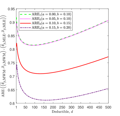
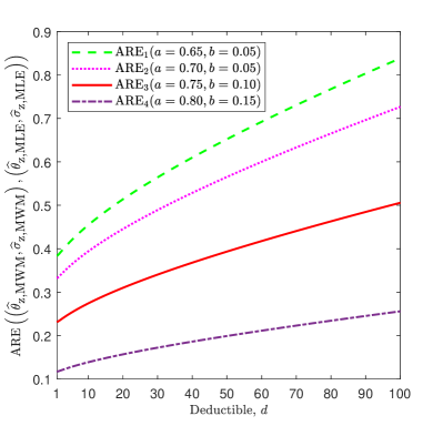
Figure 4.1: $\mbox{ARE}\left(\left(\widehat{\theta}_{\mbox{\tiny v,MWM}},\widehat{\sigma}_{\mbox{\tiny v,MWM}}\right),\left(\widehat{\theta}_{\mbox{\tiny v,MLE}},\widehat{\sigma}_{\mbox{\tiny v,MLE}}\right)\right)$ curves as functions of policy deductible $d$ and with fixed policy limit $u=5.96\times 10^{3}$, where $v=y$ (left panel) and $v=z$ (right panel), respectively, represent the payments $Y$ and $Z$ data scenarios from $\mbox{LN}(1,4,2)$ distribution.

Clearly the ARE expressions given by Eqs. (4.23), and (4.30) are functions of $d$, $u$, the parameters to be estimated, and the trimming and wisnorizing proportions. It is important to note here that those AREs for completely observed ground-up loss data set do not depend on the parameters to be estimated, see, e.g., Brazauskas et al. (2009) and Zhao et al. (2018a). As functions of policy deductible, $d$, those AREs are visualized in Figure 4.1 for some selected winsorizing proportions satisfying Case III as specified in Section 4.1 for payment $Y$ and Case 6 as considered in Section 4.2 for payment $Z$.

For payment $Y$ (Figure 4.1, left panel), the ARE curves for the left winsorizing proportions $a\in\{0.00,0.05\}$ with fixed right winsorizing proportion $b=0.10$ do not have significant difference, but when the left winsorizing proportion is increasing then the ARE values are going down. Since the ARE curves do not have consistent patter (either increasing or decreasing) as functions of $d$, this makes the practical interpretation of those curves more difficult.

On the other hand, for payment $Z$, the ARE curves are consistently increasing functions of $d$ (Figure 4.1, right panel). This is because higher the value of $d$ implies the narrower support for exact loss observations (which are bigger than $d$ and smaller than $u$) which eventually yields the smaller variance of MWM estimators.

5 Simulation Study

This section supplements the theoretical results we developed in Section 4 via simulation. The main goal is to assess the size of the sample such that the finite estimators are free from bias (given that the estimators are asymptotically unbiased), justify the asymptotic normality, and their finite sample relative efficiencies (REs) to reach the corresponding AREs. To compute RE of MWM estimators we use MLE as a benchmark. Thus, the definition of ARE given by equation (4.5) for finite sample performance translates to:

$$RE(\mbox{MWM, MLE})=\frac{\text{asymptotic variance of MLE estimator}}{\text{small-sample variance of a competing MWM estimator}},$$ (5.1)

where the numerator is as defined in (4.5) and the denominator is given by:

$$\left(\mbox{det}\begin{bmatrix}E\left[\left(\widehat{\theta}-\theta\right)^{2}\right]&E\left[\left(\widehat{\theta}-\theta\right)\left(\widehat{\sigma}-\sigma\right)\right]\\[15.0pt] E\left[\left(\widehat{\theta}-\theta\right)\left(\widehat{\sigma}-\sigma\right)\right]&E\left[\left(\widehat{\sigma}-\sigma\right)^{2}\right]\end{bmatrix}\right)^{1/2}.$$

5.1 Study Design

From a ground-up lognormal distribution $F_{W}(w_{0}=1,\theta=4,\sigma=2)$, we generate 10,000 samples of a specified length $n$ using Monte Carlo. For each sample we estimate the parameters of $F$ using various MTM and MWM estimators and then compute the average mean and RE of those 10,000 estimates. The standardized ratio $\hat{\theta}/\theta$ that we report is defined as the average of 10,000 estimates divided by the true value of the parameter that we are estimating. The standard error is standardized in a similar manner.

Table 5.1: Selection of trimming and winsorizing proportions.

Method		MLE	MTM/MWM
Payments $Y$	$a$	–	0.05	0.10	0.15	0.00	0.00	0.00
	$b$	–	0.05	0.10	0.15	0.05	0.10	0.25
Payments $Z$	$a$	–	0.10	0.15	0.25	0.10	0.10	0.10
	$b$	–	0.10	0.15	0.25	0.05	0.15	0.25

We observe the performance of different methods of estimation for lognormal distribution. The simulation study is designed with following parameters:

1. Sample size: $n=100,\,500,\,1000,\,\infty$

2. Coinsurance rate: $c=1$.

3. Truncation and censoring thresholds for both variables $Y$ and $Z$:

   • $d=3$ (corresponding to about 5% left-truncation);

   • $u_{1}=5.96\times 10^{3}$ (corresponding to about 1% right-censoring);

   • $u_{2}=1.54\times 10^{3}$ (corresponding to about 5% right-censoring).

4. Selection of trimming and winsorizing proportions:

   • As mentioned in Section 4.1, for payments $Y$, the trimmed- and winsorized-estimators are derived under the condition that $0\leq a<1-b\leq s^{*}$ (i.e., Case II). In simulations, however, the proportion $s^{*}$ is random, which can easily result in violations of the specified condition. If $s^{*}$ is estimated empirically, i.e., by replacing $F$ with its empirical estimator $\widehat{F}_{n}$, then the variance of such estimator is equal to $\sigma_{\hat{s}^{*}}^{2}=\frac{{s}^{*}\left(1-{s}^{*}\right)}{n}$. Thus, to minimize the number of possible violations, the right trimming proportion $b$ is chosen to satisfy the following inequality:

     $$1-b \leq s^{*}-2\sigma_{\hat{s}^{*}},$$ (5.2)

     and, to demonstrate the difference between sufficiently and insufficiently robust trimmed- and winsorized-estimators, some values of $b$ are chosen to violate the condition $1-b\leq s^{*}-2\sigma_{\hat{s}^{*}}.$

   • Again, as mentioned in Section 4.2 and for payments $Z$, the equivalent condition is $F(d)\leq a<1-b\leq F(u)$. Similar arguments as those for payments $Y$ lead to $\sigma_{\hat{F}_{n}(d)}^{2}=\frac{F(d)(1-F(d))}{n}$ and $\sigma_{\hat{F}_{n}(u)}^{2}=\frac{F(u)(1-F(u))}{n}$. In this case, the left and right trimming/winsorizing proportions $a$ and $b$, respectively, are chosen such that

     $$F(d)+2\sigma_{\hat{F}_{n}(d)}\leq a\quad\mbox{and}\quad 1-b\leq F(u)-2\sigma_{\hat{F}_{n}(u)}.$$

5. Estimators of $\theta$ and $\sigma$: MLE, MTM, and MWM estimators with the trimming and Winsorizing proportions as specified in Table 5.1.

Table 5.2: Lognormal payment-per-payment actuarial loss scenario, $LN(w_{0}=1,\theta=4,\sigma=2)$ with $d=3$ and two selected values of right-censoring point $u$. The entries are mean values based on 10,000 samples.

	Proportion		$n=100$				$n=500$				$n=1000$				$n\to\infty$
	$a$	$b$	MWM		MTM		MWM		MTM		MWM		MTM		MWM		MTM
			$\widehat{\theta}/\theta$	$\widehat{\sigma}/\sigma$	$\widehat{\theta}/\theta$	$\widehat{\sigma}/\sigma$	$\widehat{\theta}/\theta$	$\widehat{\sigma}/\sigma$	$\widehat{\theta}/\theta$	$\widehat{\sigma}/\sigma$	$\widehat{\theta}/\theta$	$\widehat{\sigma}/\sigma$	$\widehat{\theta}/\theta$	$\widehat{\sigma}/\sigma$	$\widehat{\theta}/\theta$	$\widehat{\sigma}/\sigma$	$\widehat{\theta}/\theta$	$\widehat{\sigma}/\sigma$
$u=5.96\times 10^{3}$	Mean values of $\widehat{\theta}/\theta$ and $\widehat{\sigma}/\sigma$.
	MLE		1.00	1.00	1.00	1.00	1.00	1.00	1.00	1.00	1.00	1.00	1.00	1.00	1.00	1.00	1.00	1.00
	0.05	0.05	1.00	0.99	0.99	1.01	1.00	1.00	1.00	1.00	1.00	1.00	1.00	1.00	1.00	1.00	1.00	1.00
	0.10	0.10	1.00	0.99	0.99	1.01	1.00	1.00	1.00	1.00	1.00	1.00	1.00	1.00	1.00	1.00	1.00	1.00
	0.15	0.15	1.00	0.99	0.99	1.01	1.00	1.00	1.00	1.00	1.00	1.00	1.00	1.00	1.00	1.00	1.00	1.00
	0.00	0.05	1.00	1.00	1.00	1.00	1.00	1.00	1.00	1.00	1.00	1.00	1.00	1.00	1.00	1.00	1.00	1.00
	0.00	0.10	1.00	1.00	1.00	1.01	1.00	1.00	1.00	1.00	1.00	1.00	1.00	1.00	1.00	1.00	1.00	1.00
	0.00	0.25	0.99	1.00	0.99	1.01	1.00	1.00	1.00	1.00	1.00	1.00	1.00	1.00	1.00	1.00	1.00	1.00
	Finite-sample efficiencies (RE) of MWMs and MTMs relative to MLEs.
	MLE		0.97		0.98		1.00		1.00		1.00		1.00		1.000		1.000
	0.05	0.05	0.92		0.88		0.95		0.92		0.95		0.92		0.945		0.913
	0.10	0.10	0.84		0.77		0.87		0.82		0.88		0.83		0.873		0.823
	0.15	0.15	0.76		0.68		0.79		0.73		0.80		0.74		0.796		0.734
	0.00	0.05	0.92		0.89		0.95		0.92		0.95		0.92		0.950		0.913
	0.00	0.10	0.86		0.80		0.89		0.84		0.90		0.84		0.892		0.841
	0.00	0.25	0.68		0.59		0.72		0.64		0.73		0.65		0.724		0.650
$u=1.54\times 10^{3}$	Mean values of $\widehat{\theta}/\theta$ and $\widehat{\sigma}/\sigma$.
	MLE		1.00	1.00	1.00	1.00	1.00	1.00	1.00	1.00	1.00	1.00	1.00	1.00	1.00	1.00	1.00	1.00
	0.05	0.05	1.00	0.98	0.99	1.00	1.00	0.99	1.00	1.00	1.00	1.00	1.00	1.00	1.00	1.00	1.00	1.00
	0.10	0.10	1.00	0.99	0.99	1.01	1.00	1.00	1.00	1.00	1.00	1.00	1.00	1.00	1.00	1.00	1.00	1.00
	0.15	0.15	1.00	0.99	0.99	1.01	1.00	1.00	1.00	1.00	1.00	1.00	1.00	1.00	1.00	1.00	1.00	1.00
	0.00	0.05	1.00	0.98	1.00	1.00	1.00	1.00	1.00	1.00	1.00	1.00	1.00	1.00	1.00	1.00	1.00	1.00
	0.00	0.10	1.00	1.00	0.99	1.01	1.00	1.00	1.00	1.00	1.00	1.00	1.00	1.00	1.00	1.00	1.00	1.00
	0.00	0.25	0.99	1.00	0.99	1.01	1.00	1.00	1.00	1.00	1.00	1.00	1.00	1.00	1.00	1.00	1.00	1.00
	Finite-sample efficiencies (RE) of MWMs and MTMs relative to MLEs.
	MLE		0.95		0.96		0.98		0.98		1.00		1.00		1.000		1.000
	0.05	0.05	1.10		0.97		1.10		0.96		1.10		0.98		0.994		0.960
	0.10	0.10	0.89		0.81		0.90		0.84		0.91		0.86		0.919		0.865
	0.15	0.15	0.80		0.71		0.82		0.75		0.83		0.77		0.837		0.772
	0.00	0.05	1.11		0.97		1.11		0.97		1.11		0.98		1.000		0.964
	0.00	0.10	0.91		0.84		0.92		0.86		0.93		0.88		0.938		0.884
	0.00	0.25	0.72		0.61		0.75		0.66		0.76		0.67		0.762		0.684

Note: The standard errors for the entire entries in this table are reported to be $\leq 0.0015$.

5.2 Convergence and Relative Bias

Table 5.3: Lognormal payment-per-loss actuarial loss scenario, $LN(w_{0}=1,\theta=4,\sigma=2)$ with $d=3$ and two selected values of right-censoring point $u$. The entries are mean values based on 10,000 samples.

	Proportion		$n=100$				$n=500$				$n=1000$				$n\to\infty$
	$a$	$b$	MWM		MTM		MWM		MTM		MWM		MTM		MWM		MTM
			$\widehat{\theta}/\theta$	$\widehat{\sigma}/\sigma$	$\widehat{\theta}/\theta$	$\widehat{\sigma}/\sigma$	$\widehat{\theta}/\theta$	$\widehat{\sigma}/\sigma$	$\widehat{\theta}/\theta$	$\widehat{\sigma}/\sigma$	$\widehat{\theta}/\theta$	$\widehat{\sigma}/\sigma$	$\widehat{\theta}/\theta$	$\widehat{\sigma}/\sigma$	$\widehat{\theta}/\theta$	$\widehat{\sigma}/\sigma$	$\widehat{\theta}/\theta$	$\widehat{\sigma}/\sigma$
$u=5.96\times 10^{3}$	Mean values of $\widehat{\theta}/\theta$ and $\widehat{\sigma}/\sigma$.
	MLE		1.00	0.99	1.00	0.99	1.00	1.00	1.00	1.00	1.00	1.00	1.00	1.00	1.00	1.00	1.00	1.00
	0.10	0.10	1.00	0.99	1.00	1.00	1.00	1.00	1.00	1.00	1.00	1.00	1.00	1.00	1.00	1.00	1.00	1.00
	0.15	0.15	1.00	0.99	1.00	1.00	1.00	1.00	1.00	1.00	1.00	1.00	1.00	1.00	1.00	1.00	1.00	1.00
	0.25	0.25	1.00	0.98	1.00	1.01	1.00	1.00	1.00	1.00	1.00	1.00	1.00	1.00	1.00	1.00	1.00	1.00
	0.10	0.05	1.00	0.99	1.00	1.00	1.00	1.00	1.00	1.00	1.00	1.00	1.00	1.00	1.00	1.00	1.00	1.00
	0.10	0.15	1.00	0.99	1.00	1.00	1.00	1.00	1.00	1.00	1.00	1.00	1.00	1.00	1.00	1.00	1.00	1.00
	0.10	0.25	1.00	0.99	1.00	1.00	1.00	1.00	1.00	1.00	1.00	1.00	1.00	1.00	1.00	1.00	1.00	1.00
	Finite-sample efficiencies (RE) of MWMs and MTMs relative to MLEs.
	MLE		0.99		1.00		1.00		1.00		1.00		1.00		1.000		1.000
	0.10	0.10	0.87		0.81		0.88		0.82		0.88		0.79		0.891		0.810
	0.15	0.15	0.78		0.71		0.80		0.72		0.79		0.70		0.791		0.712
	0.25	0.25	0.60		0.53		0.61		0.54		0.61		0.52		0.603		0.534
	0.10	0.05	0.92		0.87		0.93		0.87		0.93		0.85		0.927		0.863
	0.10	0.15	0.83		0.76		0.84		0.77		0.84		0.75		0.854		0.761
	0.10	0.25	0.74		0.66		0.75		0.68		0.75		0.66		0.776		0.667
$u=1.54\times 10^{3}$	Mean values of $\widehat{\theta}/\theta$ and $\widehat{\sigma}/\sigma$.
	MLE		1.00	1.00	1.00	1.00	1.00	1.00	1.00	1.00	1.00	1.00	1.00	1.00	1.00	1.00	1.00	1.00
	0.10	0.10	1.00	0.99	1.00	1.00	1.00	1.00	1.00	1.00	1.00	1.00	1.00	1.00	1.00	1.00	1.00	1.00
	0.15	0.15	1.00	0.99	1.00	1.00	1.00	1.00	1.00	1.00	1.00	1.00	1.00	1.00	1.00	1.00	1.00	1.00
	0.25	0.25	1.00	0.98	1.00	1.01	1.00	1.00	1.00	1.00	1.00	1.00	1.00	1.00	1.00	1.00	1.00	1.00
	0.10	0.05	1.00	0.98	1.00	1.00	1.00	1.00	1.00	1.00	1.00	1.00	1.00	1.00	1.00	1.00	1.00	1.00
	0.10	0.15	1.00	0.99	1.00	1.00	1.00	1.00	1.00	1.00	1.00	1.00	1.00	1.00	1.00	1.00	1.00	1.00
	0.10	0.25	1.00	0.99	1.00	1.00	1.00	1.00	1.00	1.00	1.00	1.00	1.00	1.00	1.00	1.00	1.00	1.00
	Finite-sample efficiencies (RE) of MWMs and MTMs relative to MLEs.
	MLE		1.00		0.97		1.02		1.02		1.03		1.03		1.000		1.000
	0.10	0.10	0.92		0.83		0.92		0.82		0.92		0.83		0.923		0.839
	0.15	0.15	0.82		0.73		0.82		0.72		0.83		0.74		0.819		0.738
	0.25	0.25	0.63		0.54		0.63		0.54		0.63		0.56		0.625		0.553
	0.10	0.05	1.05		0.91		1.05		0.89		1.04		0.90		0.961		0.894
	0.10	0.15	0.87		0.77		0.87		0.77		0.87		0.79		0.884		0.788
	0.10	0.25	0.77		0.68		0.77		0.68		0.78		0.69		0.804		0.690

Note: The standard errors for the entire entries in this table are reported to be $\leq 0.0013$.

Simulation results of both MTM and MWM are recorded in Tables 5.2 (for payment-per-payment variable $Y$) and 5.3 (for payment-per-payment variable $Z$). The entries of the last column ($n\to\infty$) represent analytic results that are included in Section 5. It helps us compare large-sample properties with small-sample properties when the deductible and policy limit occur.

The relative bias is defined as the ratio of the expectation of parameter estimate to its true value, thus making the value of one the target. As is seen in Table 5.2, all MWM and MTM estimators successfully estimate both the log-location parameter $\mu$ and scale parameter $\sigma$. Indeed, they practically become unbiased for samples of size $n\geq 500$. The situation is similar in Table 5.3. Furthermore, we notice that the simulated RE’s of these estimators for $n\geq 500$ are almost identical to the corresponding ARE’s for large policy limit $u=5.96\times 10^{3}$. When $u$ moves to $1.54\times 10^{3}$, however, the RE’s of MWM in finite size samples are far from corresponding ARE for $b=0.05$ and this is because the condition (5.2) is violated which leads to poor parameter estimation.

5.3 Risk Measure Sensitivity

In this section, we study sensitivity of our estimators to an outlier $\mathcal{O}$ that is placed at various locations within the sample ranging from $d$ to $u$. The outlier can be viewed as a new observation for the original sample, thus when all the estimates are recomputed, they can be plotted against the location of $\mathcal{O}$ resulting in sensitivity curves. To see what impact the outlier has on the riskiness of the ground-up variable, $W\sim LN(w_{0},\theta,\sigma)$ as defined in Section 2, we consider four risk measures: Mean $(\mu$, $\mu_{\mbox{\tiny MTM}}$, and $\mu_{\mbox{\tiny MWM}})$, Value at Risk $(\mbox{VaR}_{p})$, Tail Value at Risk $(\mbox{VTaR}_{p})$, and Proportional Hazard Distortion Risk Measure $(\mbox{PHDRM}_{p})$. Each of them is a special case of the general distortion risk measure

$$R(F_{W}) =\int_{0}^{1}F_{W}^{-1}(v)J(v)\,dv+\sum_{j=1}^{m}\beta_{j}F_{W}^{-1}(p_{j}),$$ (5.3)

where $F_{W}$ is the cdf of $W$. More details are referred in Serfling (1980), p. 265 and Frees (2017). The specific components of each risk measure given by equation (5.3) are listed in Table 5.4.

Table 5.4: Mean, Value at Risk $(\mbox{VaR}_{p})$, Tail Value at Risk $(\mbox{VTaR}_{p})$, and Proportional Hazard Distortion Risk Measure $(\mbox{PHDRM}_{p})$ in general risk measure format.

	Risk Measure	$J(v)$	$m$	$(\beta_{1},\beta_{2})$	$(p_{1},p_{2})$	$R(F_{W})$
Mean	$\mu$	1	0	-	-	$w_{0}+e^{\theta+\frac{1}{2}\sigma^{2}}$
	$\mu_{\mbox{\tiny MTM}}$	$\dfrac{1}{\tau}\mathds{1}\{a\leq v\leq\bar{b}\}$	0	-	-	$w_{0}+\tau^{-1}e^{\theta+\frac{1}{2}\sigma^{2}}\cdot$
						$\hskip 10.84006pt\left(\Phi\left(\Phi^{-1}(\bar{b})-\sigma\right)-\Phi\big{(}\Phi^{-1}(a)-\sigma\big{)}\right)$
	$\mu_{\mbox{\tiny MWM}}$	$\mathds{1}\{a\leq v\leq\bar{b}\}$	2	$(a,b)$	$(a,\bar{b})$	$w_{0}+e^{\theta}\cdot\bigg{[}ae^{\sigma\Phi^{-1}(a)}+be^{\sigma\Phi^{-1}(\bar{b})}+e^{\frac{1}{2}\sigma^{2}}\cdot$
						$\hskip 10.84006pt\left(\Phi\left(\Phi^{-1}(\bar{b})-\sigma\right)-\Phi\left(\Phi^{-1}(a)-\sigma\right)\right)\bigg{]}$
Other	$\mbox{VaR}_{p}$	0	1	-	$p_{1}=p\in[0,1)$	$w_{0}+e^{\theta+\sigma\Phi^{-1}(p)}$
	$\mbox{TVaR}_{p}$	$\dfrac{1}{\bar{p}}\mathds{1}\{p\leq v\leq 1\}$	0	-	-	$w_{0}+\dfrac{e^{\theta+\frac{1}{2}\sigma^{2}}}{\bar{p}}\Phi\left(\sigma-\Phi^{-1}(p)\right)$
	$\mbox{PHDRM}_{p}$	$p(1-v)^{p-1}$	0	-	-	$\displaystyle{\int_{0}^{\infty}\left[1-\Phi\left(\frac{\ln{w}-\theta}{\sigma}\right)\right]^{p}\,dw}$

Note: When $m=0,(\beta_{1},\beta_{2})$ and $(p_{1},p_{2})$ are not available and the empty spaces are filled with $``-^{\prime\prime}$.

5.3.1 Payments Y

A sample of size 100 generated from $W\sim LN(w_{0}=1,\theta=4,\sigma=2)$ with $d=100$ (about 62% left truncation), $u=2.5\times 10^{3}$ (about 3% right censoring) is given in Appendix B, Table B.1. The parameters $\theta$ and $\sigma$ are first estimated via MLE, $T_{1}\equiv MTM(a=0.00,b=0.10)$, $T_{2}\equiv MTM(a=0.00,b=0.15)$, $T_{3}\equiv MTM(a=0.00,b=0.20)$, $W_{1}\equiv MWM(a=0.00,b=0.10)$, $W_{2}\equiv MWM(a=0.00,b=0.15)$, $W_{3}\equiv MWM(a=0.00,b=0.20)$, by placing an outlier $\mathcal{O}$ at various locations between $d=100$ and $u=2500$ (or, in terms of $Y$, between $0$ and $2400$). The right trimming/winsorizing proportion $a$ and $b$ is chosen to satisfy the condition $1-b\leq s^{*}=0.93$. Since $F_{W}(d)$ is already approximately 62%, the left trimming/winsorizing proportion $a$ is fixed as $0$. The corresponding risk measure sensitivity curves are then reported in Figure 5.1.

The stability exhibited by the curves of $T3-$ and $W3-$ estimators is about 63% of possible data range ($63\%\approx(2500-1000)/(2500-100)$), and this width narrows down to about 33% for $T_{1},W_{1}$ and to about 58% for $T_{2},W_{2}$ when the proportion $b$ tends to be small. Besides, all MTM and MWM risks measures of $\mu,\text{VaR}_{0.99},\text{TVaR}_{0.99}$ and $\text{PHDRM}_{0.99}$ remain stable when the new observation $\mathcal{O}$ occurs near the upper boundary of 2500, whereas the equivalent estimates based on MLE show a sudden jump/drop at that right-censoring threshold.

As seen in the sensitivity curve, MTM and MWM based $\text{VaR}_{0.99}$ and $\text{TVaR}_{0.99}$ values are much closer to the theoretical targets (marked as dashed lines in Figure 5.1) than those of MLE results at most locations. This indicates that without the more extreme observations, MTM and MWM estimators can still capture the behavior of shortfall above the 99% threshold and generate adequate risk control measures.

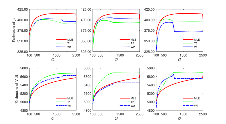
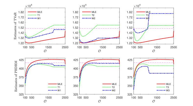
Figure 5.1: Sensitivity curves of MLE (solid curve), trimmed (dotted curve), and winsorized (dash-dot curve) estimators of $\mu=404.43$, $\mbox{VaR}_{0.99}=5,726.56$, $\mbox{TVaR}_{0.99}=15,011.80$, and $\mbox{PHDRM}_{0.99}=416.74$ as the outlier $\mathcal{O}$ increases from $100$ to $2,500$ under the payment-per-payment data scenario. In each plot, the theoretical target is marked as dashed line.

5.3.2 Payments Z

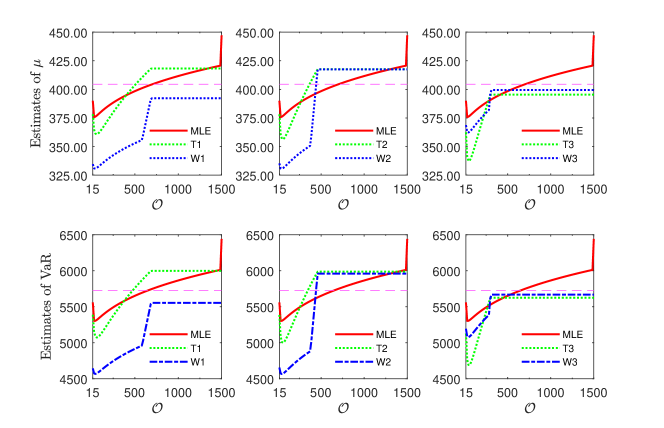
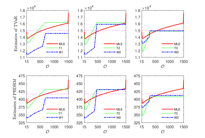
Figure 5.2: Sensitivity curves of MLE (solid curve), trimmed (dotted curve), and winsorized (dash-dot curve) estimators of $\mu=404.43$, $\mbox{VaR}_{0.99}=5,726.56$, $\mbox{TVaR}_{0.99}=15,011.80$, and $\mbox{PHDRM}_{0.99}=416.74$ as the outlier $\mathcal{O}$ increases from $15$ to $1,500$ under the payment-per-loss data scenario. In each plot, the theoretical target is marked as dashed line.

A sample of size 100 generated from $W\sim LN(w_{0}=1,\theta=4,\sigma=2)$ with $d=15$ (about 25% left truncation), $u=1.5\times 10^{3}$ (about 5% right censoring) is given in Appendix B, Table B.2. Again, the parameters $\theta$ and $\sigma$ are first estimated via MLE, $T_{1}\equiv MTM(a=0.25,b=0.10)$, $T_{2}\equiv MTM(a=0.25,b=0.15)$, $T_{3}\equiv MTM(a=0.25,b=0.20)$, $W_{1}\equiv MWM(a=0.25,b=0.10)$, $W_{2}\equiv MWM(a=0.25,b=0.15)$, $W_{3}\equiv MWM(a=0.25,b=0.20)$, by placing an outlier $\mathcal{O}$ at various locations between $d=15$ and $u=1500$ (or, in terms of $Z$, between $0$ and 1,485). The corresponding risk measure sensitivity curves are then reported in Figure 5.2. As mentioned in Section 4.2, the trimming/winsorizing proportion $a$ and $b$ are chosen to satisfy the condition $0\leq F_{W}(d)\leq a<1-b\leq F_{W}(u)\leq 1.$

It is obvious that the pattern of the four risk measures follows the same direction. The MLE based sensitivity curves are influenced by all locations of $\mathcal{O}$; in particular, a larger jump near the upper boundary of 1500. This indicates that even an extreme claim has been censored to the threshold, it still highly affects the estimation procedure of the maximum likelihood method, leading to an over- or under-estimate of risk pricing in actuarial application.

With regard to the two robust estimators $MTM$ and $MWM$, the placement of $\mathcal{O}$ at $d=15$ causes fluctuation for all estimates of $\mu,\text{VaR}_{0.99},\text{TVaR}_{0.99}$ and $\text{PHDRM}_{0.99}$. That is because the chosen $a$ almost “break down” against the left truncation point $d$. On the other hand, since all of the MTM and MWM estimators are designed to be sufficiently robust against upper data, we observe the stability of each corresponding risk measure from the right-hand side. Moreover, as trimming/winsorizing proportion $b$ increases, the stability range becomes wider. For example, $b=0.1$ maintain stability for about 57% of the upper data range $(57\%\approx(1500-650)/(1500-15))$ while $b=0.15$ and $b=0.20$ have those about 70% and 84%, respectively. In particular, the premium pricing and risk control are unaffected when a new extreme claim (outlier) merges into the portfolio. More importantly, with appropriate proportions $a$ and $b$ (i.e., $a=0.25,b=0.20$), $T3$ and $W3$ based values are closer moving toward and even coinciding with the theoretical targets (marked as dashed lines in Figure 5.2).

From Figures 5.1 and 5.2, we clearly observed that MLE estimated statistics are highly volatile even for truncated and/or censored dataset with sudden jumps at the censored thresholds. A simple remedy for this volatile issue can be achieved via the robust MTM- or MWM-estimators. These methods simply remove the impact of point masses accumulated by MLE at the censored thresholds. For example, as seen in Table 4.1 (see the entries inside the rectangular box), out of $LN(1,4,2)$ distribution, if 10% of the sample data are right censored and if we simply winsorize those 10% censored data values, i.e., $a=0,\ b=10\%$ then the sensitivity curves turn out to be more stable and at the same time the asymptotic relative efficiency is still maintained at 99.90% level. The corresponding asymptotic relative efficiency for MTM is maintained at 94.20% which is still close to 1.

All above - mentioned trends of sensitivity behavior (Figures 5.1 and 5.2) do not depend on the risk level. That means, if we switch the risk threshold from $p=0.99$ to $p=0.95$ or some other level, the corresponding risk measure statistics will change but the fundamental pattern of sensitivity curves still remain the same.

6 Real Data Illustrations

In this section, we apply the MWM, MTM and MLE (both stand-alone lognormal as well as two composite models) to analyze 1500 indemnity losses in the United States provided by Insurance Service Office, Inc, which has been widely studied in the actuarial literature (see, e.g., Frees and Valdez, 1998, Beirlant et al., 2004, Michael et al., 2020) and are available in the R package copula with data name loss, Kojadinovic and Yan (2010). Our goal is to investigate what effect initial assumptions and parameter estimation methods have on model fit and corresponding insurance contract pricing.

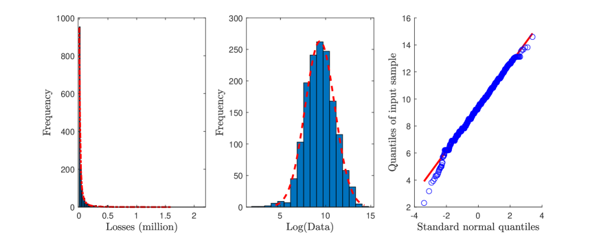
Figure 6.1: The histograms of the top 1500 indemnity losses. Left panel: Original data. Middle panel: Log-transformed data. Right panel: Log-normal QQ plot.

A preliminary diagnostics (see in Figure 6.1), which we have based on the histogram and normal QQ-plot of the log-transformed losses, shows that lognormal distribution may provide an adequate fit to indemnity losses. Thus, the usage of developed composite as well as adaptive models are illustrated on this loss data and the impact of trimming/winsorizing proportions on the lognormal model performance will be examined thoroughly.

Table 6.1: Payment-per-payment $Y$, payment-per-loss $Z$, transformation, and number of loss amounts with data truncation and censoring for the U.S. indemnity losses.

Payment Type	Left Truncation		Right Censoring		# of loss amounts within each range
	$d$	$t$	$u$	$T$	$(0,d]$	$(d,u)$	$[u,\infty)$	Total
$Y$	500	6.2146	$10^{5}$	11.5129	-	1299	152	1451
$Z$	500	6.2146	$10^{5}$	11.5129	49	1299	152	1500

Note: $t=\log(d-w_{0}),$ and $T=\log(u-w_{0})$.

We consider estimation of the loss severity component of the pure premium for an insurance benefit that equals to the amount by which an indemnity loss ($W$) exceeds 500 (deductible, $d=500$) dollars with a maximum benefit of 100,000 dollars (policy limit, $u=10^{5}$). Without loss of generality, we assume that $c=1$ since the asymptotic variances of all the estimators investigated in this paper do not depend on the coinsurance factor $c$. The corresponding lognormal payment-per-payment and payment-per-loss variables have the formulas as defined by $F_{Y}$ and $f_{Y}$, $F_{Z}$ and $f_{z}$, respectively, from Poudyal (2021a), Section 2. Their transformations, and number of loss observations within each range of contract are also summarized in Table 6.1.

Without considering the robustness, we first compare the performance of three candidate models – stand-alone lognormal, composite LNPaI, and composite LNGPD (mentioned in Section 3.3), and determine the benchmark for further study of adaptive robust estimators. In this stage, all the parameters are estimated via maximum likelihood estimation and the corresponding statistics and performance indicators (such as Negative log-likelihood and Akakie Information Criterion) are illustrated in Table 6.2.

Table 6.2: MLE fitted composite models with some selection criterion for the 1500 US indemnity payment-per-payment, $Y$, and payment-per-loss, $Z$, data scenarios.

Payments	Estimators	$\widehat{\theta}$	$\widehat{\sigma}$	$\widehat{x}_{0}$	$\widehat{\alpha}$	$\widehat{\lambda}$	$w$	NLL	AIC	LEV
$Y$	LN	9.43	1.59	-	-	-	1	14,456.28	28,916.55	2.675
	LNPaI	9.35	1.49	82,282	0.885	-	0.878	14,454.19	28,914.37	2.661
	LNGDP	9.33	1.47	14,244	1.020	11,700	0.541	14,454.22	28,916.44	2.663
$Z$	LN	9.39	1.64	-	-	-	1	14,674.03	29,352.06	2.600
	LNPaI	9.30	1.58	99,999	0.883	-	0.895	14,673.95	29,353.90	2.595
	LNGDP	9.92	1.83	4,239	1.027	11,961	0.258	14,673.44	29,354.87	2.582

Note: $x_{0}$: Location that separates Lognormal and Pareto models. $w$: proportion of Lognormal distribution. NLL: Negative log-likelihood. AIC: AIC criterion. The limited expected value LEV is in $10^{4}$.

Obviously, there is not much improvement either in NLL or in AIC going from stand-alone lognormal model to either LNPaI or to LNGPD. The percentage changes are clearly way smaller than $0.50\%$. Therefore, at least out of this data illustration, what we can conclude is that for payment-per-payment and payment-per-loss, that is, for truncated and/or censored loss data scenarios, the stand-alone lognormal model is equally powerful to model those data scenarios as the competing composite models. This is because the composite models are specially more powerful to provide a good fit to the entire range of the loss data given that there are large losses with small probabilities, but for payments $Y$ and $Z$ those large losses are already censored at the policy limit, $u$. Hence, due to the simplicity of the distribution, the stand-alone lognormal model is the optimal option to serve as the MLE benchmark in the following step of methodology comparisons.

Next, considering model robustness, we discuss the model fit of the MTM and MWM estimators in $PPY$ and $PPZ$ scenarios when policy deductible and policy limit are included in the risk pricing. In Section 1, we mentioned that MWM for truncated and censored loss data is an adaptive estimation procedures. This is the right place to describe why we call MWM an adaptive estimation procedure. First, for payment $Y$, the MWM estimators as well as their asymptotic results are based on the assumption of $0\leq a<1-b\leq s^{*}\leq 1$. Then, an obvious challenge in estimation procedures is to maintain the condition $0\leq a<1-b\leq s^{*}\leq 1$ both empirically and parametrically. Initially, we set

$$\hat{s}_{\mbox{\tiny E}}^{*}:=\dfrac{F_{n}(T)-F_{n}(t)}{1-F_{n}(t)}={n_{1}}/{n},\quad\mbox{where $F_{n}$ is the empirical cdf},$$

and choose $b$ such that $1-b\leq\hat{s}_{\mbox{\tiny E}}^{*}$. But after estimating $\widehat{\theta}_{\mbox{\tiny y,MWM}}$ and $\widehat{\sigma}_{\mbox{\tiny y,MWM}}$, it could be the case that

$$\hat{s}_{\mbox{\tiny P}}^{*}:=\dfrac{\widehat{F}_{X}(T)-\widehat{F}_{X}(t)}{1-\widehat{F}_{X}(t)}<1-b,\quad\mbox{where $\widehat{F}_{X}$ is the estimated parametric cdf},$$

which is unsatisfactory for statistical inferences as it violates the assumption (Case II from Section 4.1). Therefore, the value of $b$ should be chosen adaptively such that $1-b\leq\min\{\hat{s}_{\mbox{\tiny E}}^{*},\hat{s}_{\mbox{\tiny P}}^{*}\}.$ Likewise, for payment $Z$, the left and right trimming proportions $a$ and $b$ are also chosen adaptively:

$$\max\{F_{n}(t),\widehat{F}_{X}(t)\}\leq a\quad\mbox{and}\quad 1-b\leq\min\{F_{n}(T),\widehat{F}_{X}(T)\}.$$

The trimming and winsorizing proportions in Tables 6.3 and 6.4 are chosen accordingly. Adaptive MTM and MWM are now, respectively, called by AMTM and AMWM for the rest of this section.

As observed in the indemnity data set, 49 losses among 1500 claims are below the deductible, and 152 losses are above the policy limit. Since our major objective is to see if the fitted model captures the behavior of the underlying distribution, it is natural to choose $a$ and $b$ proportions that fluctuate across left-truncation (deductible) and right censored (policy limit), separately. In addition, to see the impact of chosen $b$ at the policy threshold ($u$) alone, we fix $a=0$ and set different values of $b$ from small $150/1451$ to large $750/1451$. The estimates of location parameter $\theta$ and scale parameter $\sigma$ for lognormal model are provided and the corresponding 95% confidence intervals are built. Further, in Tables 6.3 and 6.4, we also provide the actuarial premiums (or call it limited expected value (LEV)) calculated as

• $\text{LEV}=\dfrac{E[W\wedge u]-E[W\wedge d]}{1-F_{W}(d)}$ for payment-per-payment; and

• $\text{LEV}=E[W\wedge u]-E[W\wedge d]$ for payment-per-loss,

where

$$E[W\wedge w]=w_{0}+e^{\theta+\frac{\sigma^{2}}{2}}\Phi\left(\dfrac{\ln{(w-w_{0})}-\theta-\sigma^{2}}{\sigma}\right)+(w-w_{0})\left[1-\Phi\left(\dfrac{\ln{(w-w_{0})}-\theta}{\sigma}\right)\right].$$

Moreover, Asymptotic Relative Efficiency (ARE) and Kolmogorov–Smirnov test (KS Test) on each base are utilized to compare the model robustness and fit accuracy of various AMWM, AMTM and MLE estimators.

Table 6.3: MLE, AMTM and AMWM estimators of $\theta$ and $\sigma$ with their corresponding asymptotic confidence intervals and estimated values of AREs for payment $Y$ data scenario.

	Estimators		$\hat{\theta}$	$\hat{\sigma}$	$\hat{s}^{\ast}$		95% CI for		LEV	$\widehat{ARE}$	KS Test
					$\hat{s}_{E}^{\ast}$	$\hat{s}_{P}^{\ast}$	$\theta$	$\sigma$			$D_{y}$	$h_{y}$
MLE			9.43	1.59	-	-	(9.34, 9.52)	(1.52, 1.67)	2.675	1.00	0.032	0
	$a$	$b$	Condition required: $1-b\leq\min\{\hat{s}_{E}^{\ast},\hat{s}_{P}^{\ast}\}$
AMWM	0.00	150/1451	9.43	1.59	0.90	0.90	(9.34, 9.52)	(1.51, 1.67)	2.671	0.99	0.033	0
	0.00	200/1451	9.43	1.58	0.90	0.90	(9.34, 9.52)	(1.50, 1.66)	2.664	0.95	0.033	0
	0.00	300/1451	9.43	1.57	0.90	0.91	(9.34, 9.52)	(1.49, 1.66)	2.656	0.88	0.034	0
	0.00	700/1451	9.45	1.58	0.90	0.90	(9.35, 9.55)	(1.46, 1.71)	2.701	0.57	0.038	1
	10/1451	150/1451	9.43	1.59	0.90	0.91	(9.34, 9.52)	(1.51, 1.66)	2.671	0.99	0.033	0
	50/1451	200/1451	9.42	1.60	0.90	0.91	(9.33, 9.51)	(1.52, 1.69)	2.672	0.95	0.030	0
	100/1451	300/1451	9.42	1.60	0.90	0.90	(9.32, 9.51)	(1.51, 1.69)	2.670	0.86	0.029	0
	650/1451	650/1451	9.37	1.61	0.90	0.91	(9.25, 9.48)	(1.35, 1.91)	2.598	0.24	0.031	0
AMTM	0.00	150/1451	9.42	1.56	0.90	0.91	(9.34, 9.51)	(1.49, 1.65)	2.634	0.94	0.034	0
	0.00	200/1451	9.42	1.55	0.90	0.91	(9.33, 9.51)	(1.47, 1.64)	2.618	0.89	0.034	0
	0.00	300/1451	9.42	1.54	0.90	0.91	(9.33, 9.50)	(1.45, 1.63)	2.591	0.80	0.034	0
	0.00	700/1451	9.37	1.47	0.90	0.93	(9.27, 9.47)	(1.35, 1.59)	2.418	0.48	0.043	1
	10/1451	150/1451	9.42	1.57	0.90	0.91	(9.33, 9.51)	(1.49, 1.65)	2.637	0.94	0.033	0
	50/1451	200/1451	9.41	1.59	0.90	0.91	(9.32, 9.50)	(1.50, 1.67)	2.640	0.89	0.030	0
	100/1451	300/1451	9.40	1.59	0.90	0.90	(9.31, 9.50)	(1.50, 1.69)	2.639	0.79	0.028	0
	650/1451	650/1451	9.26	2.09	0.90	0.85	(8.96, 9.56)	(1.56, 2.81)	3.038	0.24	0.064	1

Note : The limited expected value LEV is in $10^{4}$.

As Tables 6.3 and 6.4 suggest, the AMWM and AMTM estimators with appropriate proportions $a$ and $b$ (i.e. $a=0,b=150/1451$ in Table 6.3 and $a=75/1500,b=150/1500$ in Table 6.4) lead to premium estimates that are close enough to that of non-robust estimator MLE. On the other hand, the scale estimate, confidence interval and LEV of AMWM and AMTM estimators that obtained with highly robust but inefficient estimators (i.e., $b=700/1451$ or $b=650/1451$) have a significant deviation from the corresponding MLE. In terms of ARE, the values of payment $Y$ depend on the unknown parameters of $\theta$ and $\sigma$ while those of payment $Z$ do not, resulting in the degree of efficiency loss varies from the former to the latter.

In addition, we note the remarkable stability of point estimates, interval estimates as well as LEV premiums based on small proportions of adaptive trimming/winsorizing when the assumed distribution is lognormal. Besides, we again observe substantial differences between AMWM and AMTM fits, in particular, for large $a$ and $b$ proportions. For example, in Table 6.3, when $a=b=650/1451$, AMWM has LEV$=2.598\times 10^{4}$ whereas AMTM has LEV$=3.038\times 10^{4}$. However, the ARE of these two estimators are almost identical, which shows that even in the worst case, the AMWM is still better than AMTM for pricing risks.

Table 6.4: MLE, AMTM and AMWM estimators of $\theta$ and $\sigma$ with their corresponding asymptotic confidence intervals and estimated values of AREs for payment $Z$ data scenario.

	Estimators		$\hat{\theta}$	$\hat{\sigma}$	$\widehat{F}_{X}(t)$	$\widehat{F}_{X}(T)$	95% CI for		LEV	$\widehat{ARE}$	KS Test
							$\theta$	$\sigma$			$D_{z}$	$h_{z}$
MLE			9.39	1.64	-	-	(9.30, 9.47)	(1.58, 1.71)	2.600	1.00	0.027	0
	$a$	$b$	Condition required:
			$\max\{\widehat{F}_{n}(t),\widehat{F}_{X}(T)\}\leq a$ and $1-b\leq\min\{\widehat{F}_{n}(t),\widehat{F}_{X}(T)\}$.
AMWM	75/1500	150/1500	9.40	1.61	0.02	0.91	(9.32, 9.48)	(1.54, 1.67)	2.585	0.97	0.031	0
	75/1500	225/1500	9.39	1.60	0.02	0.91	(9.31, 9.48)	(1.53, 1.67)	2.567	0.93	0.031	0
	75/1500	375/1500	9.38	1.58	0.02	0.91	(9.30, 9.47)	(1.51, 1.66)	2.533	0.83	0.031	0
	75/1500	750/1500	9.38	1.57	0.02	0.91	(9.28, 9.48)	(1.48, 1.67)	2.519	0.59	0.031	0
	150/1500	150/1500	9.39	1.63	0.03	0.90	(9.30, 9.47)	(1.56, 1.70)	2.592	0.93	0.026	0
	225/1500	225/1500	9.39	1.62	0.03	0.90	(9.30, 9.47)	(1.55, 1.70)	2.578	0.83	0.027	0
	375/1500	375/1500	9.38	1.61	0.02	0.91	(9.29, 9.47)	(1.52, 1.70)	2.552	0.64	0.027	0
	700/1500	700/1500	9.40	2.26	0.08	0.82	(9.26, 9.54)	(1.87, 2.74)	3.140	0.17	0.095	1
AMTM	75/1500	150/1500	9.38	1.62	0.03	0.91	(9.30, 9.47)	(1.55, 1.69)	2.570	0.92	0.027	0
	75/1500	225/1500	9.38	1.61	0.02	0.91	(9.30, 9.47)	(1.54, 1.69)	2.558	0.86	0.027	0
	75/1500	375/1500	9.38	1.60	0.02	0.91	(9.29, 9.46)	(1.53, 1.69)	2.544	0.76	0.027	0
	75/1500	750/1500	9.36	1.59	0.02	0.91	(9.26, 9.47)	(1.49, 1.70)	2.506	0.52	0.028	0
	150/1500	150/1500	9.38	1.63	0.03	0.90	(9.30, 9.47)	(1.55, 1.70)	2.575	0.86	0.026	0
	225/1500	225/1500	9.38	1.63	0.03	0.90	(9.29, 9.46)	(1.55, 1.72)	2.573	0.76	0.026	0
	375/1500	375/1500	9.38	1.61	0.02	0.91	(9.29, 9.47)	(1.50, 1.71)	2.551	0.57	0.027	0
	700/1500	700/1500	9.38	2.36	0.09	0.82	(9.23, 9.52)	(1.92, 2.91)	3.172	0.16	0.107	1

Note: The limited expected value LEV is in $10^{4}$.

For hypothesis testing purpose for the various fitted models, we use the Kolmogorov-Smirnov (KS) test statistic. The KS test statistic for payments $Y$ and $Z$ data sets are, respectively, defined as (see, e.g., Klugman et al., 2019, p. 360):

$$D_{y} :=\max_{0<y\leq c(T-t)}\left|F_{n}(y)-\widehat{F}_{Y}(y)\right|;$$ (6.1)

$$D_{z} :=\max_{0\leq z\leq c(T-t)}\left|F_{n}(z)-\widehat{F}_{Z}(z)\right|,$$ (6.2)

where $\widehat{F}_{Y}$ and $\widehat{F}_{Z}$ are the the estimated cdf of $F_{Y}$ and $F_{Z}$, respectively. For each fitted model, the corresponding KS test statistics $\{D_{y},D_{z}\}$ and the decision $\{h_{y},h_{z}\}$ of the hypothesis test are given in the last two columns of Tables 6.3 and 6.4 where $h_{y},h_{z}=0$ indicates that the lognormal model is plausible and $h_{y},h_{z}=1$ means that the the lognormal model is rejected at the significance level of $5\%$.

7 Conclusion

In this paper, we have introduced and developed a new estimation procedure – method of winsorized moments (MWM) – for robust fitting of truncated and censored lognormal distributions, which are appropriate for insurance payment-per-payment and payment-per-loss data. Large-sample properties of the MWM estimators have been established, and their small-sample performance has been investigated through simulations and compared to that of the main competitor (method of trimmed moments, MTM) and the benchmark MLE. Among the three methods, MLE is not robust whereas MTM and MWM are both robust and exhibit similar robustness properties. In terms of efficiency, MLE is most efficient, of course, and MWM consistently outperforms MTM under the lognormal model with policy deductible and limit. Moreover, as the sample size increases, finite-sample measures of the estimators’ performance approach their asymptotic counterparts. Further, a sensitivity study has been conducted to gauge MWM’s, MTM’s, and MLE’s response to a single outlier (new extreme observation) that is placed at various locations within the sample ranging from the point of left-truncation (deductible) to that of right-censoring (policy limit). It has been found that MLE-based sensitivity curves are influenced by all locations of $\mathcal{O}$ with the most dramatic effect when outlier is placed at the censoring threshold. Finally, the numerical examples based on 1500 U.S. indemnity losses have revealed that evaluation of the net premiums using adaptively computed right-trimming and right-winsorizing proportion for AMTM and AMWM, respectively, leads to reasonable results. By using theses 1500 U.S. indemnity losses, it is also demonstrated that, specifically for truncated and censored data, the composite models do not provide much predictive power compared to the corresponding competing stand-alone severity model.

Appendix A Auxiliary Results

Recall that, for $0\leq s\leq 1$, we define $\bar{s}=1-s$ and $\Delta_{s}:=\Phi^{-1}\left(s+\bar{s}\Phi(\gamma)\right)$.

1. The expressions for $c_{y,k}$, $1\leq k\leq 4$ used in Section 4.1 are given by:

   $$c_{y,k}\equiv c_{y,k}(\Phi,a,b,\gamma)=a\Delta_{a}^{k}+\int_{a}^{\bar{b}}\Delta_{s}^{k}\,ds+b\Delta_{\bar{b}}^{k},$$

   and consequently the corresponding expressions for $c_{k}$ used in Section 4.2 are computed as follows:

   $$c_{k}\equiv c_{k}(\Phi,a,b)=\lim_{\gamma\to-\infty}c_{y,k}=a\left[\Phi^{-1}\left(a\right)\right]^{k}+\int_{a}^{\bar{b}}\left[\Phi^{-1}\left(s\right)\right]^{k}\,ds+b\left[\Phi^{-1}\left(\bar{b}\right)\right]^{k}.$$

2. Following the appendix of Zhao et al. (2018a), the expressions presented in the entries of the variance-covariance matrix $\bf{\Sigma}_{y}$ from Section 4.1 are as follows:

   $$c_{y,1}^{*} =c_{y,2}-c_{y,1}^{2}-a\dfrac{\partial(c_{y,2}-c_{y,1}^{2})}{\partial a}-b\dfrac{\partial(c_{y,2}-c_{y,1}^{2})}{\partial b}+a\bar{a}\left(\dfrac{\partial c_{y,1}}{\partial a}\right)^{2}+b\bar{b}\left(\dfrac{\partial c_{y,1}}{\partial b}\right)^{2}-2ab\dfrac{\partial c_{y,1}}{\partial a}\dfrac{\partial c_{y,1}}{\partial b},$$

   $$2c_{y,2}^{*} =c_{y,3}-c_{y,1}\cdot c_{y,2}-a\dfrac{\partial(c_{y,3}-c_{y,1}c_{y,2})}{\partial a}-b\dfrac{\partial(c_{y,3}-c_{y,1}\cdot c_{y,2})}{\partial b}$$

   $$\quad+a\bar{a}\dfrac{\partial c_{y,1}}{\partial a}\dfrac{\partial c_{y,2}}{\partial a}+b\bar{b}\dfrac{\partial c_{y,1}}{\partial b}\dfrac{\partial c_{y,2}}{\partial b}-ab\left(\dfrac{\partial c_{y,1}}{\partial a}\dfrac{\partial c_{y,2}}{\partial b}+\dfrac{\partial c_{y,1}}{\partial b}\dfrac{\partial c_{y,2}}{\partial a}\right),$$

   $$4c_{y,3}^{*} =c_{y,4}-c_{y,2}^{2}-a\dfrac{\partial(c_{y,4}-c_{y,2}^{2})}{\partial a}-b\dfrac{\partial(c_{y,4}-c_{y,2}^{2})}{\partial b}+a\bar{a}\left(\dfrac{\partial c_{y,2}}{\partial a}\right)^{2}+b\bar{b}\left(\dfrac{\partial c_{y,2}}{\partial b}\right)^{2}-2ab\dfrac{\partial c_{y,2}}{\partial a}\dfrac{\partial c_{y,2}}{\partial b},$$

   where the involved derivatives are listed below:

   $$\dfrac{\partial c_{y,k}}{\partial a} = \Delta_{a}^{k}+\dfrac{ak\Delta_{a}^{k-1}}{\phi(\Delta_{a})}\bar{\Phi}(\gamma)-\Delta_{a}^{k}=a\bar{\Phi}(\gamma)\dfrac{k\Delta_{a}^{k-1}}{\phi(\Delta_{a})},\qquad\dfrac{\partial c_{y,k}}{\partial b}=-b\bar{\Phi}(\gamma)\dfrac{k\Delta_{\bar{b}}^{k-1}}{\phi(\Delta_{\bar{b}})},$$

   $$c_{y,k}\,c_{y,j} = a^{2}\Delta_{a}^{k+j}+ab\Big{(}\Delta_{a}^{k}\Delta_{b}^{j}+\Delta_{a}^{j}\Delta_{b}^{k}\Big{)}+b^{2}\Delta_{b}^{k+j}+\Big{(}a\Delta_{a}^{k}+b\Delta_{b}^{k}\Big{)}\int_{a}^{\bar{b}}\Delta_{s}^{j}\,ds$$

   $$+\Big{(}a\Delta_{a}^{j}+b\Delta_{b}^{j}\Big{)}\int_{a}^{\bar{b}}\Delta_{s}^{k}\,ds+\left(\int_{a}^{\bar{b}}\Delta_{s}^{k}\,ds\right)\left(\int_{a}^{\bar{b}}\Delta_{s}^{j}\,ds\right),$$

   $$\dfrac{\partial\left(c_{y,k}\,c_{y,j}\right)}{\partial a} = c_{y,j}\dfrac{\partial c_{y,k}}{\partial a}+c_{y,k}\dfrac{\partial c_{y,j}}{\partial a}=a\bar{\Phi}(\gamma)\dfrac{k\Delta_{a}^{k-1}}{\phi(\Delta_{a})}c_{y,j}+a\bar{\Phi}(\gamma)\dfrac{j\Delta_{a}^{j-1}}{\phi(\Delta_{a})}c_{y,k}$$

   $$= \dfrac{a\bar{\Phi}(\gamma)}{\phi(\Delta_{a})}\left[k\Delta_{a}^{k-1}c_{y,j}+j\Delta_{a}^{j-1}c_{y,k}\right],$$

   $$\dfrac{\partial\left(c_{y,k}\,c_{y,j}\right)}{\partial b} = c_{y,j}\dfrac{\partial c_{y,k}}{\partial b}+c_{y,k}\dfrac{\partial c_{y,j}}{\partial b}=-b\bar{\Phi}(\gamma)\dfrac{k\Delta_{\bar{b}}^{k-1}}{\phi(\Delta_{\bar{b}})}c_{y,j}-b\bar{\Phi}(\gamma)\dfrac{j\Delta_{\bar{b}}^{j-1}}{\phi(\Delta_{\bar{b}})}c_{y,k}$$

   $$= -\dfrac{b\bar{\Phi}(\gamma)}{\phi(\Delta_{\bar{b}})}\left[k\Delta_{\bar{b}}^{k-1}c_{y,j}+j\Delta_{\bar{b}}^{j-1}c_{y,k}\right].$$

3. Similarly, the expressions used in Equation (4.31) are such that $\displaystyle c_{k}^{*}=\lim_{\gamma\to-\infty}c_{y,k}^{*}$ and are given by:

   $$c_{1}^{*} =c_{2}-c_{1}^{2}-a\dfrac{\partial(c_{2}-c_{1}^{2})}{\partial a}-b\dfrac{\partial(c_{2}-c_{1}^{2})}{\partial b}+a\bar{a}\left(\dfrac{\partial c_{1}}{\partial a}\right)^{2}+b\bar{b}\left(\dfrac{\partial c_{1}}{\partial b}\right)^{2}-2ab\dfrac{\partial c_{1}}{\partial a}\dfrac{\partial c_{1}}{\partial b},$$

   $$2c_{2}^{*} =c_{3}-c_{1}\cdot c_{2}-a\dfrac{\partial(c_{3}-c_{1}c_{2})}{\partial a}-b\dfrac{\partial(c_{3}-c_{1}\cdot c_{2})}{\partial b}$$

   $$\qquad\quad+a\bar{a}\dfrac{\partial c_{1}}{\partial a}\dfrac{\partial c_{2}}{\partial a}+b\bar{b}\dfrac{\partial c_{1}}{\partial b}\dfrac{\partial c_{2}}{\partial b}-ab\left(\dfrac{\partial c_{1}}{\partial a}\dfrac{\partial c_{2}}{\partial b}+\dfrac{\partial c_{1}}{\partial b}\dfrac{\partial c_{2}}{\partial a}\right),$$

   $$4c_{3}^{*} =c_{4}-c_{2}^{2}-a\dfrac{\partial(c_{4}-c_{2}^{2})}{\partial a}-b\dfrac{\partial(c_{4}-c_{2}^{2})}{\partial b}+a\bar{a}\left(\dfrac{\partial c_{2}}{\partial a}\right)^{2}+b\bar{b}\left(\dfrac{\partial c_{2}}{\partial b}\right)^{2}-2ab\dfrac{\partial c_{2}}{\partial a}\dfrac{\partial c_{2}}{\partial b},$$

   where the involved derivatives are listed below:

   $$\dfrac{\partial c_{k}}{\partial a} = \dfrac{ka\left[\Phi^{-1}(a)\right]^{k-1}}{\phi\left(\Phi^{-1}(a)\right)},\qquad\dfrac{\partial c_{k}}{\partial b}=-\dfrac{kb\left[\Phi^{-1}\left(\bar{b}\right)\right]^{k-1}}{\phi\left(\Phi^{-1}\left(\bar{b}\right)\right)},$$

   $$\dfrac{\partial\left(c_{k}\,c_{j}\right)}{\partial a} = \dfrac{a}{\phi\left(\Phi^{-1}(a)\right)}\left[k\left[\Phi^{-1}(a)\right]^{k-1}c_{j}+j\left[\Phi^{-1}(a)\right]^{j-1}c_{k}\right],$$

   $$\dfrac{\partial\left(c_{k}\,c_{j}\right)}{\partial b} = -\dfrac{b}{\phi\left(\Phi^{-1}\left(\bar{b}\right)\right)}\left[k\left[\Phi^{-1}\left(\bar{b}\right)\right]^{k-1}c_{j}+j\left[\Phi^{-1}\left(\bar{b}\right)\right]^{j-1}c_{k}\right].$$

Appendix B Simulated Data for Risk Measure Sensitivity Analysis

70.89	290.60	47.22	100.36	411.36	1374.10	1736.60	28.12	207.47	349.15
465.04	10.41	6.12	96.41	340.27	114.82	391.35	1036.80	30.69	391.35
426.90	132.63	64.22	2400.00	213.66	257.07	849.73	34.64	275.32	2257.90
742.44	1059.80	556.32	25.60	2400.00	12.62	275.32	1288.30	2400.00	65.85
1014.30	232.99	76.06	104.39	610.90	92.54	1403.90	1647.10	216.80	239.70
116.97	29.40	279.09	2400.00	1718.30	207.47	5.08	232.99	3.02	1048.20
132.63	149.42	367.44	2400.00	260.65	132.63	104.39	928.74	76.06	618.03
625.24	970.69	54.718	45.77	670.02	198.41	3.02	223.18	2400.00	14.88
81.39	110.58	603.83	33.31	358.20	34.64	275.32	6.12	25.60	340.27
86.88	2098.60	110.58	530.62	53.19	67.52	50.18	56.26	358.20	24.36

Table B.1: Payment $Y$ Sensitivity Analysis Simulated Data.

30.21	272.88	0	336.39	99.19	284.59	43.92	120.16	0	445.00
6.07	0	45.09	41.65	5.09	78.67	31.11	1.63	0	186.15
0	805.80	17.79	569.51	0	38.93	200.66	64.97	10.76	64.18
2.76	0	0	0	54.65	1081.60	1479.77	0	1479.77	102.64
319.30	5.47	9.79	19.42	0	106.19	0	458.98	33.90	0
0	1479.77	0	361.80	10.27	124.25	1421.20	0	87.40	0
90.49	0	220.88	1479.77	92.60	6.47	0	50.65	15.05	67.37
2.76	1479.77	530.06	86.39	358.06	0	1479.77	29.77	13.91	670.75
127.04	196.41	50.65	503.52	12.02	0	26.41	30.21	56.04	8.18
124.25	0	08	0	0	218.54	0	145.02	48.74	3.80

Table B.2: Payment $Z$ Sensitivity Analysis Simulated Data.

References

- Beirlant et al. (2004) Beirlant, J., Goegebeur, Y., Teugels, J., and Segers, J. (2004). Statistics of Extremes: Theory and Applications. Wiley Series in Probability and Statistics. John Wiley & Sons, Ltd., Chichester.
- Blostein and Miljkovic (2019) Blostein, M. and Miljkovic, T. (2019). On modeling left-truncated loss data using mixtures of distributions. Insurance: Mathematics & Economics, 85, 35–46.
- Brazauskas et al. (2009) Brazauskas, V., Jones, B.L., and Zitikis, R. (2009). Robust fitting of claim severity distributions and the method of trimmed moments. Journal of Statistical Planning and Inference, 139(6), 2028–2043.
- Brazauskas and Kleefeld (2016) Brazauskas, V. and Kleefeld, A. (2016). Modeling severity and measuring tail risk of Norwegian fire claims. North American Actuarial Journal, 20(1), 1–16.
- Chernoff et al. (1967) Chernoff, H., Gastwirth, J.L., and Johns, Jr., M.V. (1967). Asymptotic distribution of linear combinations of functions of order statistics with applications to estimation. Annals of Mathematical Statistics, 38(1), 52–72.
- Cohen (1950) Cohen, Jr., A.C. (1950). Estimating the mean and variance of normal populations from singly truncated and doubly truncated samples. Annals of Mathematical Statistics, 21(4), 557–569.
- Cohen (1951) Cohen, Jr., A.C. (1951). On estimating the mean and variance of singly truncated normal frequency distributions from the first three sample moments. Annals of the Institute of Statistical Mathematics, 3, 37–44.
- Cooray and Ananda (2005) Cooray, K. and Ananda, M.M.A. (2005). Modeling actuarial data with a composite lognormal-Pareto model. Scandinavian Actuarial Journal, 2005(5), 321–334.
- Delong et al. (2021) Delong, L.u., Lindholm, M., and Wüthrich, M.V. (2021). Gamma mixture density networks and their application to modelling insurance claim amounts. Insurance: Mathematics & Economics, 101, 240–261.
- Fabián (2001) Fabián, Z. (2001). Induced cores and their use in robust parametric estimation. Communications in Statistics: Theory and Methods, 30(3), 537–555.
- Fabián (2008) Fabián, Z. (2008). New measures of central tendency and variability of continuous distributions. Communications in Statistics: Theory and Methods, 37(1-2), 159–174.
- Fabián (2010) Fabián, Z. (2010). Scalar score function and score correlation. Technical Report 1077, Institute of Computer Science, Academy of Sciences of the Czech Republic.
- Frees (2017) Frees, E. (2017). Insurance portfolio risk retention. North American Actuarial Journal, 21(4), 526–551.
- Frees and Valdez (1998) Frees, E.W. and Valdez, E.A. (1998). Understanding relationships using copulas. North American Actuarial Journal, 2(1), 1–25.
- Fung (2021) Fung, T.C. (2021). Maximum weighted likelihood estimator for robust heavy-tail modelling of finite mixture models. Available at arXiv:2108.01356.
- Goffard and Laub (2021) Goffard, P.O. and Laub, P.J. (2021). Approximate Bayesian computations to fit and compare insurance loss models. Insurance: Mathematics & Economics, 100, 350–371.
- Gui et al. (2021) Gui, W., Huang, R., and Lin, X.S. (2021). Fitting multivariate Erlang mixtures to data: a roughness penalty approach. Journal of Computational and Applied Mathematics, 386, 113216, 17.
- Hewitt et al. (1979) Hewitt, C.C., Jr., and Lefkowitz, B. (1979). Methods for fitting distributions to insurance loss data. Proceedings of the Casualty Actuarial Society, volume LXVI, pages 139–160. Casualty Actuarial Society, VA.
- Klugman et al. (2019) Klugman, S.A., Panjer, H.H., and Willmot, G.E. (2019). Loss Models: From Data to Decisions. Fifth edition. John Wiley & Sons, Hoboken, NJ.
- Kojadinovic and Yan (2010) Kojadinovic, I. and Yan, J. (2010). Modeling multivariate distributions with continuous margins using the copula R package. Journal of Statistical Software, 34(9), 1–20.
- Michael et al. (2020) Michael, S., Miljkovic, T., and Melnykov, V. (2020). Mixture modeling of data with multiple partial right-censoring levels. Advances in Data Analysis and Classification. ADAC, 14(2), 355–378.
- Miljkovic and Grün (2016) Miljkovic, T. and Grün, B. (2016). Modeling loss data using mixtures of distributions. Insurance: Mathematics & Economics, 70, 387–396.
- Nadarajah and Bakar (2014) Nadarajah, S. and Bakar, S.A.A. (2014). New composite models for the Danish fire insurance data. Scandinavian Actuarial Journal, 2014(2), 180–187.
- Pigeon and Denuit (2011) Pigeon, M. and Denuit, M. (2011). Composite lognormal-Pareto model with random threshold. Scandinavian Actuarial Journal, 2011(3), 177–192.
- Poudyal (2021a) Poudyal, C. (2021a). Robust estimation of loss models for lognormal insurance payment severity data. ASTIN Bulletin, 51(2), 475–507.
- Poudyal (2021b) Poudyal, C. (2021b). Truncated, censored, and actuarial payment-type moments for robust fitting of a single-parameter Pareto distribution. Journal of Computational and Applied Mathematics, 388, 113310, 18.
- Punzo et al. (2018) Punzo, A., Bagnato, L., and Maruotti, A. (2018). Compound unimodal distributions for insurance losses. Insurance: Mathematics & Economics, 81, 95–107.
- Scollnik (2007) Scollnik, D.P.M. (2007). On composite lognormal-Pareto models. Scandinavian Actuarial Journal, 2007(1), 20–33.
- Serfling (2002) Serfling, R. (2002). Efficient and robust fitting of lognormal distributions. North American Actuarial Journal, 6(4), 95–109.
- Serfling (1980) Serfling, R.J. (1980). Approximation Theorems of Mathematical Statistics. John Wiley & Sons, New York.
- Shah and Jaiswal (1966) Shah, S.M. and Jaiswal, M.C. (1966). Estimation of parameters of doubly truncated normal distribution from first four sample moments. Annals of the Institute of Statistical Mathematics, 18, 107–111.
- Stehlík et al. (2010) Stehlík, M., Potocký, R., Waldl, H., and Fabián, Z. (2010). On the favorable estimation for fitting heavy tailed data. Computational Statistics, 25(3), 485–503.
- Tomarchio and Punzo (2020) Tomarchio, S.D. and Punzo, A. (2020). Dichotomous unimodal compound models: application to the distribution of insurance losses. Journal of Applied Statistics, 47(13-15), 2328–2353.
- Tukey (1960) Tukey, J.W. (1960). A survey of sampling from contaminated distributions. Contributions to Probability and Statistics, pages 448–485. Stanford University Press, Stanford, CA.
- van der Vaart (1998) van der Vaart, A.W. (1998). Asymptotic Statistics. Cambridge University Press, Cambridge.
- Zhao et al. (2018a) Zhao, Q., Brazauskas, V., and Ghorai, J. (2018a). Robust and efficient fitting of severity models and the method of Winsorized moments. ASTIN Bulletin, 48(1), 275–309.
- Zhao et al. (2018b) Zhao, Q., Brazauskas, V., and Ghorai, J. (2018b). Small-sample performance of the MTM and MWM estimators for the parameters of log-location-scale families. Journal of Statistical Computation and Simulation, 88(4), 808–824.