Dynamics of non-Gaussian fluctuations in model A

Abstract

Motivated by the experimental search for the QCD critical point we perform simulations of a stochastic field theory with purely relaxational dynamics (model A). We verify the expected dynamic scaling of correlation functions. Using a finite size scaling analysis we obtain the dynamic critical exponent $z=2.026(56)$. We investigate time dependent correlation functions of higher moments $M^{n}(t)$ of the order parameter $M(t)$ for $n=1,2,3,4$. We obtain dynamic scaling with the same critical exponent $z$ for all $n$, but the relaxation constant depends on $n$. We also study the relaxation of $M^{n}(t)$ after a quench, where the simulation is initialized in the high temperature phase, and the dynamics is studied at the critical temperature $T_{c}$. We find that the evolution does not follow simple scaling with the dynamic exponent $z$, and that it involves an early time rise followed by late stage relaxation.

I Introduction

Fluctuation observables are an important tool in the experimental search for a possible critical endpoint in the QCD phase diagram Stephanov et al. (1998); Bzdak et al. (2020); Bluhm et al. (2020); An et al. (2022). The main idea is that the system created in a heavy ion collision can be described as a strongly interacting fluid, which is characterized by a local temperature as well as baryon, isospin, and strangeness chemical potentials. In heavy ion experiments there are a number of control parameters, such as the beam energy, the system size, the impact parameter and the rapidity of the observed particles, that affect the trajectory of the strongly interacting fluid and the location of the freezeout surface in the phase diagram of QCD. If the freezeout surface is close to a critical point, then this will manifest itself as an enhancement of event-by-event fluctuations in a number of observables, for example in the variance of the number of net protons. It was recognized that it may be advantageous to consider higher order cumulants, such as the skewness and kurtosis Ejiri et al. (2006); Stephanov (2009); Asakawa et al. (2009); Stephanov (2011); Friman et al. (2011), because these observables show a stronger dependence on the correlation length near the critical point, and they may exhibit a non-monotonic behavior as a function of the beam energy.

A heavy ion collision is a short-lived, very dynamic, event. This implies that non-equilibrium phenomena, such as critical slowing down and memory effects cannot be ignored Berdnikov and Rajagopal (2000); Nahrgang et al. (2019); Akamatsu et al. (2019); Bluhm et al. (2020); An et al. (2022). In terms of the experimental observation of critical behavior this fact may indeed be beneficial, as memory effects imply that fluctuations observables at freezeout encode the possible transit of a critical point earlier during the evolution. However, non-equilibrium effects also complicate the interpretation of experimental results, because critical slowing down limits the overall magnitude of critical effects, and non-equilibrium phenomena affect individual observables in different ways. As a consequence, we may not be able to map different cumulants at freezeout onto a single point in the phase diagram.

Previous work on this issue has mostly focused on the time evolution of the two-point function Stephanov and Yin (2018); Akamatsu et al. (2019). Notable exceptions include the work in Mukherjee et al. (2015); Nahrgang et al. (2019); An et al. (2021); Sogabe and Yin (2021), but these studies use approximations to truncate the hierarchy of correlation functions, or solve the dynamics in a restricted geometry. Our goal in this work is to study the time evolution and equilibration time of non-Gaussian fluctuations in a 3+1 dimensional framework. For simplicity we will consider the critical behavior of a non-conserved order parameter in a relaxational theory without couplings to a conserved energy or momentum density. This is known as model A in the classification of Hohenberg and Halperin Hohenberg and Halperin (1977). A possible critical endpoint in the QCD phase diagram is believed to be in the universality class of model H Son and Stephanov (2004), and the chiral critical behavior in the vicinity of a second order chiral phase transition is in the universality class of model G Rajagopal and Wilczek (1993); Nakano et al. (2012); A. Florio and Teaney (2022). In the present work we study the dynamics of model A on a three dimensional lattice. Studies of kinetic Ising models are reported in Hasenbusch (2020) (and references therein) and relativistic stochastic models have been investigated in Schweitzer et al. (2020, 2021).

II Model A

For a single component field the dissipative dynamics is described by

$$\frac{\partial\phi(t,\vec{x})}{\partial t}=-\Gamma\,\frac{\delta{\cal H}}{\delta\phi(t,\vec{x})}+\zeta(t,\vec{x}),$$ (1)

where $\Gamma$ is the relaxation rate and ${\cal H}$ is the Hamiltonian

$${\cal H}=\int d^{d}x\left[\frac{1}{2}(\nabla\phi)^{2}+\frac{1}{2}m_{0}^{2}\phi^{2}(t,\vec{x})+\frac{1}{4}\lambda\phi^{4}(t,\vec{x})-h(t,\vec{x})\phi(t,\vec{x})\right]\,,$$ (2)

and $h$ is an external field. The noise term $\zeta(t,\vec{x})$ describes the interaction with microscopic degrees of freedom. Usually it is modelled as a random field with zero mean and white noise spectrum

$$\langle\zeta(t,\vec{x})\zeta(t^{\prime},\vec{x}^{\prime})\rangle=2T\,\Gamma\,\delta(\vec{x}-\vec{x}^{\prime})\delta(t-t^{\prime})\,.$$ (3)

In this work we will discretize the Hamiltonian on a spatial lattice with lattice spacing $a$, adopting units so that $a=1$. We use periodic boundary conditions in our simulations. We write the lattice field as $\phi(t,\vec{x})\to\phi(\vec{x})$, where we have dropped the explicit dependence on $t$ to simplify the notation, and $\vec{x}=a\vec{n}$ with $\vec{n}$ a vector with integer components. We have

$${\cal H}=\sum_{\vec{x}}\left[\frac{1}{2}\sum_{\mu=1}^{d}(\phi(\vec{x}+\hat{\mu})-\phi(\vec{x}))^{2}+\frac{1}{2}m_{0}^{2}\phi^{2}(\vec{x})+\frac{1}{4}\lambda\phi^{4}(\vec{x})-h\phi(\vec{x})\right]\,.$$ (4)

The vector $\hat{\mu}$ has a unit size and only one non-zero entry at $\mu$-th position. E.g. for $\mu=2$ and $d=3$, $\hat{\mu}=(0,1,0)$. In the following we will need the change in the Hamiltonian as we make a local update of the field. Changing the field $\phi_{\rm old}\to\phi_{\rm new}$ at a fixed position $\vec{x}$ leads to

$$\Delta{\cal H} =d(\phi^{2}_{\rm new}(\vec{x})-\phi^{2}_{\rm old}(\vec{x}))-(\phi_{\rm new}(\vec{x})-\phi_{\rm old}(\vec{x}))\sum_{\mu=1}^{d}\left(\phi(\vec{x}+\hat{\mu})+\phi(\vec{x}-\hat{\mu})\right)$$

$$+\frac{1}{2}m_{0}^{2}(\phi^{2}_{\rm new}(\vec{x})-\phi^{2}_{\rm old}(\vec{x}))+\frac{1}{4}\lambda(\phi^{4}_{\rm new}(\vec{x})-\phi^{4}_{\rm old}(\vec{x}))-h(\phi_{\rm new}(\vec{x})-\phi_{\rm old}(\vec{x}))\,.$$ (5)

Following the recent work of Florio et al. A. Florio and Teaney (2022) we will simulate the stochastic evolution using a Metropolis algorithm. Similar methods have been employed in the Langevin simulation described in Moore (2000) and in kinetic Ising models Hasenbusch (2020). The time-dynamics is modelled using a fixed time step size $\Delta t$. We sweep through the lattice using a checkerboard pattern. At every site $\vec{x}$ we perform a trial update

$$\phi_{\rm new}(\vec{x})=\phi_{\rm old}(\vec{x})+\sqrt{2\Delta t\Gamma}\xi\,.$$ (6)

Here $\xi$ is a random number sampled from a Gaussian distribution with zero mean and unit variance. The trial update is accepted, that is

$$\phi(t+\Delta t,\vec{x})=\phi_{\rm new}(\vec{x})\,$$ (7)

with probability $P={\rm min}(1,e^{-\Delta{\cal H}})$. If the trial update is rejected, the field at this lattice site remains unchanged

$$\phi(t+\Delta t,\vec{x})=\phi(t,\vec{x})\,.$$ (8)

Note that for the purely relaxational model studied here the relaxation rate sets the unit of time. For simplicity we set $\Gamma=1$, and time is measured in units of the inverse relaxation constant.

III Statics

The time evolution of a generic initial condition via the stochastic differential equation (1) will generate an ensemble characterized by the probability distribution $P(\phi)\sim\exp(-{\cal H}/T)$. This ensemble can be used to study static properties of the Ising Hamiltonian in equ. (2). As a first step, we determine the critical value $m_{c}^{2}<0$ of the mass parameter for a given value of $\lambda$. Here, we have chosen $\lambda=4$.

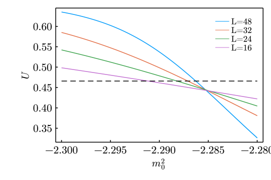
Figure 1: The Binder cumulant as a function of the control parameter $m_{0}^{2}$ for different values of the box size $L$. The dashed line show the universal value of $U$ in the infinite volume limit, determined in Hasenbusch et al. (1998). An extrapolation of the location of the crossing of our Monte Carlo results with the dashed line to $L\to\infty$ gives $m_{c}^{2}=-2.28587(7)$.

In order to locate $m_{c}^{2}$ from simulations in a finite volume we use the Binder cumulant method. We define the magnetization

$$M(t)=\frac{1}{L^{3}}\sum_{\vec{x}}\phi(t,\vec{x})$$ (9)

and compute the time average

$$\langle O\rangle=\frac{\sum_{t}O(t)}{\sum_{t}1}.$$ (10)

Here, the sum should only be taken over configurations that are generated after the initial equilibration time, and that are separated by more than the autocorrelation time. In practice, we perform measurements every 100 Monte Carlo sweeps through the entire lattice. Near the critical value $m_{c}^{2}$ fluctuation observables such as $\langle M^{2}\rangle$ and $\langle M^{4}\rangle$ show peaks, but in a finite volume simulation the location of these peaks is different from the infinite volume value of $m_{c}^{2}$. Binder observed that at the true critical point $m_{c}^{2}$ the leading finite volume corrections to the Binder cumulant

$$U=1-\frac{\langle M^{4}\rangle}{3\langle M^{2}\rangle^{2}}$$ (11)

cancel Binder (1981). This means that we can use finite volume calculations of $U$ to accurately locate the critical point of the infinite system.

In practice we perform a series of simulations on a coarse grid in $m_{0}^{2}$, and then use reweighting to more accurately determine the critical value of $m_{0}^{2}$. Reweighting for a given observable $O[M]$ is performed around ${\bar{m}}_{0}^{2}$ via

$$\langle O[M]\rangle_{m_{0}^{2}}=\frac{\sum_{t}e^{-\frac{\delta m^{2}}{2}\sum_{\vec{x}}\phi^{2}(t,\vec{x})}O[M(t)]}{\sum_{t}e^{-\frac{\delta m^{2}}{2}\sum_{\vec{x}}\phi^{2}(t,\vec{x})}}\,.$$ (12)

Here $\delta m^{2}=m_{0}^{2}-{\bar{m}}^{2}_{0}$ and the field configurations are sampled at ${\bar{m}}_{0}^{2}$. Therefore in the code one can simply save $M(t)$ and $\sum_{\vec{x}}\phi^{2}(t,\vec{x})$ for many $t$; the analysis is then can be executed separately and independently for different target $m_{0}^{2}$. Large values of $|\delta m^{2}|$ (even of order 0.1) are not only problematic because of reweighting but also due to large values of the sum $\sum_{\vec{x}}\phi^{2}(t,\vec{x})$ and the corresponding underflow/overflow while evaluating the exponent. Instead one can simply compute

$$\langle O[M]\rangle_{m_{0}^{2}}=\frac{\sum_{t}e^{-\frac{\delta m^{2}}{2}(\sum_{\vec{x}}\phi^{2}(t,\vec{x})-c)}O[M(t)]}{\sum_{t}e^{-\frac{\delta m^{2}}{2}(\sum_{\vec{x}}\phi^{2}(t,\vec{x})-c)}}$$ (13)

where $c$ is a constant defined by

$$c=\left\langle\sum_{\vec{x}}\phi^{2}(t,\vec{x})\right\rangle_{{\bar{m}}_{0}^{2}}\,.$$ (14)

The approximate value of critical $m_{c}^{2}$ was determined by running the simulations on coarse lattices, see Fig. 1. Then longer simulation were done at single value of the parameter ${\bar{m}}_{0}^{2}=-2.288$, and reweighting technique was used to recover the dependence on $m_{0}^{2}$ in the vicinity of ${\bar{m}}_{0}^{2}$.

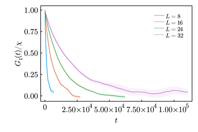
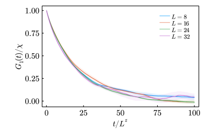
Figure 2: Correlation function $G_{1}(t)/\chi$ as a function of time for various system sizes at the critical point. Left panel: Correlation functions as a function of time $t$. Right panel: Correlation functions as a function of the a function of the scaled time variable $t/L^{z}$.

The crossing points between the solid lines in Fig. 1 indicate that $m_{c}^{2}\simeq-2.285$. A very precise value of $m_{c}^{2}$ can be obtained using the strategy adopted in A. Florio and Teaney (2022). We make use of the universal value of the Binder cumulant at the critical point, $U_{c}=0.4658$ Hasenbusch et al. (1998). This value is shown as the dashed line in Fig. 1. Then we find the location $m_{\crossproduct}^{2}(L)$ at which the Binder cumulant $U(m^{2},L)$ intersects the line $U=U_{c}$. Finite size scaling predicts $m_{\crossproduct}^{2}(L)=m_{c}^{2}+CL^{-1/\nu-\omega}$. Using the values of the critical exponents $\omega=0.8303$ and $\nu=0.62999(5)$ from El-Showk et al. (2014) to fit the data for $L=24$, 32, 48 we get $m_{c}^{2}=-2.28587(7)$.

IV Dynamics

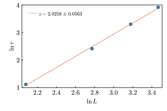
Figure 3: Relation between the decay time $\tau$ extracted from the correlation function $G_{1}(t)$ and the linear box size $L$. The line shows the best fit with $z=2.0258$.

An important feature of the dynamics near the critical point is dynamical scaling. It implies that near the critical point the correlation function $G_{1}(t,x)=\langle\phi(0,0)\phi(t,x)\rangle$ behaves as $G_{1}(t,x)\sim f(t/\tau,x/\xi)$, where $f$ is a universal function, $\xi$ is the correlation length, and $\tau\sim\xi^{z}$ is the correlation time. The quantity $z$ is known as the dynamic critical exponent. The dynamic exponent can be determined by studying the scaling of the relaxation time of a mode with wave number $k\sim\xi^{-1}$ as a function of the correlation length. Here, we use a simpler method, which is based on finite size scaling Zinn-Justin (2002). At zero external magnetic field, the correlation time in a finite volume of linear size is

$$\tau(T,L)=L^{z}f_{\tau}\left(\Delta TL^{1/\nu}\right)\,.$$ (15)

We work sufficiently close to the critical point to approximate $f\left(\Delta TL^{1/\nu}\right)$ by $f\left(0\right)$. In the case of model A, the prediction of the $\varepsilon$ expansion is Zinn-Justin (2002); Antonov and Vasil’ev (1984); Folk and Moser (2006)

$$z=2+R\,\eta,\quad R=\left(6\ln\frac{4}{3}-1\right)\left(1-\varepsilon\cdot 0.1885+...\right)$$ (16)

with $\eta=3\varepsilon^{2}/162$. The conformal bootstrap gives $\eta\approx 0.0363$ Alday and Zhiboedov (2016). Using the latter value we obtain $z\simeq 2.02$. Dynamic scaling is expected to extend to higher $n$-point functions Zinn-Justin (2002), and to correlation functions of higher dimension operators. In the following we will consider the correlation functions

$$G_{n}(t)=\langle M^{n}(0)M^{n}(t)\rangle,$$ (17)

where $M(t)$ is the magnetization defined in equ. (9), and for even $n$ we subtract the asymptotic value, $G_{n}(t)\to G_{n}(t)-\langle M^{n}(0)\rangle^{2}$. Note that $G_{1}(t)$ is the volume integral of the function $G_{1}(t,x)$ defined above.

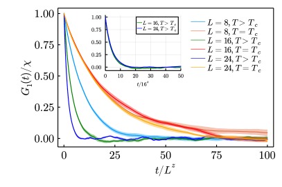
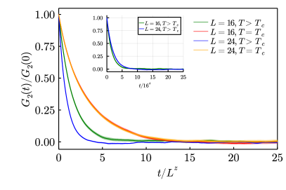
Figure 4: $G_{1}(t)/\chi$ (left panel) and $G_{2}(t)/G_{2}(0)$ (right panel) as a function of time for various system sizes $L$ at and above the critical point. The figure shows time in units of $L^{z}$, and the inset displays the correlation function with no scaling applied.

In Fig. 2 we show the two-point function of the magnetization $G_{1}(t)$ for different volumes at zero external field and directly at the critical point $m_{c}^{2}$. In the right panel we have scaled the time $t$ by a factor $L^{z}$, using the theory prediction $z=2.02$. We observe that the data collapse to a universal function. In Fig. 3 we show the scaling of the fitted decay constant $\tau$ with the box size $L$. The best fit value of the dynamic exponent is $z=2.0258\pm 0.0563$, in good agreement with the theoretical expectation. We also obtain $\ln f_{\tau}(0)=-3.13\pm 0.16$, where $f_{\tau}(x)$ is defined in equ. (15).

In Fig. 4 we show that dynamical scaling does not hold away from the critical point. The left and right panel show the two-point functions of $M$ and $M^{2}$, $G_{1}(t)$ and $G_{2}(t)$, normalized to their value at $t=0$. The $T>T_{c}$ data were taken at $m_{0}^{2}=-2.20$. The main figure show the correlation function scaled by $L^{z}$, and the inset shows unscaled correlation functions. We observe that both $G_{1}$ and $G_{2}$ exhibit dynamic scaling at $T_{c}$, but that for $T>T_{c}$ the correlation functions are essentially independent of volume.

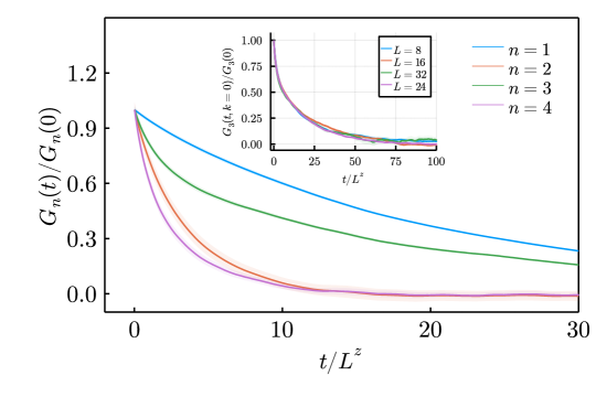
Figure 5: $G_{n}(t)/G_{n}(0)$ as a function of time $t$ for a fixed system size $L$ at the critical point. The inset demonstrates that dynamic scaling is present for higher order correlations functions. Here, we choose $G_{3}(t)$ as an illustration, and consider several different linear box sizes $L=8,16,24,32$.

The correlation functions of $M^{n}(t)$ for $n=1,2,3,4$ are shown in Fig. 5 and Fig. 6. The inset of Fig. 5 shows that dynamic scaling continues to hold. Here, we focus on $G_{3}(t)$ and show that data collapse takes place when $t$ is scaled by $L^{z}$. Similar results hold for $G_{2}(t)$ and $G_{4}(t)$. We observe that there is a pattern where correlation functions of even powers of $M(t)$ decay at a similar rate, and the same is true for correlation functions of odd powers of $M(t)$. Fig. 6 shows that this pattern holds both at $T_{c}$ and above $T_{c}$. Note that dynamic scaling is broken at $T>T_{c}$. The observed pattern is consistent with the existence of partially disconnected contributions $G_{3}(t)\sim\langle M^{2}\rangle^{2}\langle M(0)M(t)\rangle$ and $G_{4}(t)\sim\langle M^{2}\rangle^{2}\langle M^{2}(0)^{2}M(t)\rangle$. Finally, we observe that the asymptotic decay of $G_{2}(t)$ and $G_{4}(t)$ is significantly faster than that of $G_{1}(t)$ and $G_{3}(t)$. An exponential fit of the asymptotic decay rate indicates that $G_{2}(t)$ decays about five times faster than $G_{1}(t).$

We have also studied the relaxation of $M^{n}(t)$ after a quench. In Fig. 7 we show $\langle M^{n}(t)\rangle$ for an ensemble of stochastic evolutions. The initial state is drawn from an ensemble generated at $T>T_{c}$, using $m_{0}^{2}=-2.20$ as in Fig. 4 and the right panel of Fig. 6. This state is evolved using the dynamic equations at the critical point. We observe that the evolution consists of at least two stages, an early time rise and a late stage relaxation. Note that the early time behavior persists in a regime $t\in[0,t_{s}]$, where $t_{s}\gg\Gamma^{-1}$ is a macroscopic time scale. Also note that the early time dynamics violates dynamic scaling. There is no data collapse if the time evolution in different volumes is scaled by $L^{z}$. Finally, we observe that both the initial evolution and the final relaxation of $M^{4}(t)$ is slower than that of $M^{2}(t)$.

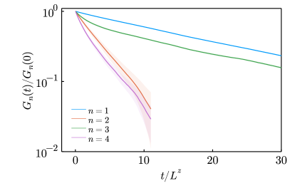
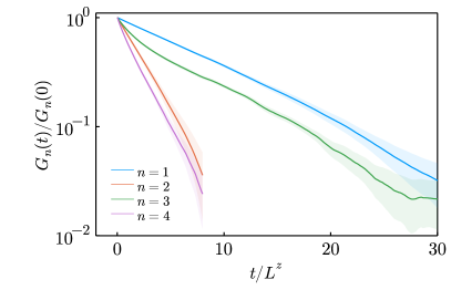
Figure 6: Left panel: This figure shows the same correlation functions as the main plot in Fig. 5, but displayed on a logarithmic scale. The curves for $n=2,4$ are terminated when the lower error band crosses zero. Right panel: Same set of correlation functions as in the left panel for $T>T_{c}$.

Breaking of dynamic scaling in the early time behavior of the order parameter after a quench to the critical regime was previously studied in Janssen et al. (1989); Ritschel and Diehl (1995); Calabrese et al. (2006). These papers characterize the early time rise of the order parameter in terms of a slip exponent $\Theta$, which is distinct from the dynamic exponent $z$. They also note that the crossover between early time evolution and late time relaxation takes place at a macroscopic time that depends on the size of the system.

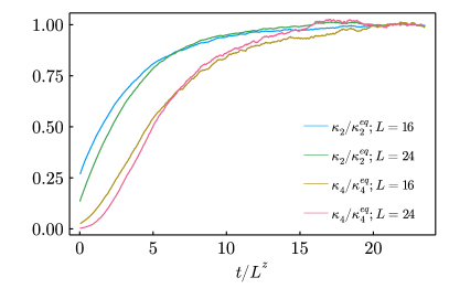
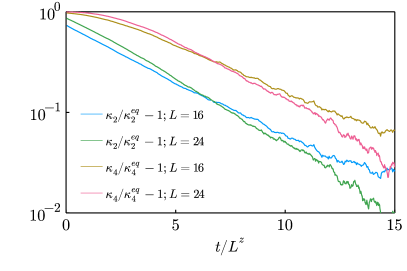
Figure 7: Left panel: Time dependence of the moments $M^{2}(t)$ and $M^{4}(t)$ of the order parameter after a quench from the high temperature phase to the the critical point. The curves are normalized to the asymptotic expectation values $\langle M^{2}\rangle$ and $\langle M^{4}\rangle$ at the critical temperature. We show results for two different linear box sizes, $L=16$ and $L=24$. Right panel: Same functions as in the left panel, but displayed on a logarithmic scale and with the asymptotic value subtracted.

V Conclusions and Outlook

We have studied the time evolution of higher moments of the order parameter in a theory with purely relaxational dynamics (model A). We used a simple Metropolis algorithm in order to simulate the stochastic dynamics, and we employed a finite size scaling analysis the measure the dynamic critical exponent. We find $z=2.026(56)$, in agreement with predictions from the $\epsilon$ expansion, and earlier numerical studies.

We have shown that correlation functions of higher moments of the order parameter are governed by the same critical exponent as the two-point function of the magnetization. However, the relaxation time and the functional form of the decay depend on the power of the order parameter. We find that quadratic and quartic moments decay faster than the order parameter, but the third moment decays on a time scale similar to the order parameter. We also studied the relaxation of powers of the order parameter after a quench. We thermalized the system at $T>T_{c}$, and determined the evolution using the dynamics at $T=T_{c}$. We find that the dynamics involves two stages, an early time increase, followed by late time relaxation to the equilibrium value at $T_{c}$. The crossover time between these two stages takes place at a macroscopic time $t_{s}\gg\Gamma^{-1}$, and the overall evolution does not satisfy simple dynamic scaling with the dynamic exponent $z$.

The methods discussed here can be generalized to models that are capture more of the dynamics in a heavy ion collisions, or other physical systems that might be of interest. In particular, there is no obstacle to considering a conserved order parameter (model B), or the coupling to the conserved momentum density (model H).