Double sampling for informatively missing data in electronic health record-based comparative effectiveness research

Abstract

Missing data arise in most applied settings and are ubiquitous in electronic health records (EHR). When data are missing not at random (MNAR) with respect to measured covariates, sensitivity analyses are often considered. These post-hoc solutions, however, are often unsatisfying in that they are not guaranteed to yield concrete conclusions. Motivated by an EHR-based study of long-term outcomes following bariatric surgery, we consider the use of double sampling as a means to mitigate MNAR outcome data when the statistical goals are estimation and inference regarding causal effects. We describe assumptions that are sufficient for the identification of the joint distribution of confounders, treatment, and outcome under this design. Additionally, we derive efficient and robust estimators of the average causal treatment effect under a nonparametric model and under a model assuming outcomes were, in fact, initially missing at random (MAR). We compare these in simulations to an approach that adaptively estimates based on evidence of violation of the MAR assumption. Finally, we also show that the proposed double sampling design can be extended to handle arbitrary coarsening mechanisms, and derive nonparametric efficient estimators of any smooth full data functional.

1 Introduction

Missing data is a well-studied problem, with researchers having a vast array of statistical methods at their disposal including inverse-probability weighting (IPW) (Seaman and White, 2013), multiple imputation (Rubin, 2004), and doubly-robust methods (Robins et al., 1994; Tsiatis, 2007). For the majority of these, the missing at random (MAR) assumption (Rubin, 1976) is, in one way or another, invoked. For settings where the MAR assumption is not viewed as plausible, methods exist based on alternative sets of identifying assumptions (e.g., Malinsky et al., 2020), availability of an instrumental variable (e.g., Sun et al., 2018) or a “shadow variable” (e.g., Miao and Tchetgen Tchetgen, 2016), sensitivity analyses (e.g., Robins et al., 2000) and the estimation of bounds (e.g., Manski, 1990). Interestingly, common to all of these methods is that they approach the task of dealing with missing data as a post-hoc challenge, that is with an exclusive focus on methods for the data at-hand.

An alternative strategy is to engage in additional data collection, referred to in this paper as double-sampling, specifically to obtain information that could either inform the plausibility of missingness assumptions or be used in an analysis to mitigate bias, or both. Such a strategy is common when addressing confounding (Borgan et al., 2018) and measurement error and/or missclassification (Carroll et al., 2006; Amorim et al., 2021), but seems to have been under-explored as a strategy for addressing missing data, (Hansen and Hurwitz, 1946; Frangakis and Rubin, 2001; Guan et al., 2018; Miao et al., 2021). Moreover, a general treatment of double sampling for missing data, or more generally coarsened data (Heitjan and Rubin, 1991), in the context of causal inference has not been developed.

One important area of biomedical and public health research where missing data is almost ubiquitous is that of studies making use of electronic health records (EHR). With large sample sizes and rich covariate information over extended periods, EHR data represent a significant and cost-effective opportunity (Haneuse and Shortreed, 2017). Furthermore, these data present a key alternative when randomized clinical trials are not feasible or could not be conducted ethically. EHR systems, however, are typically designed to support clinical and/or billing activities, and not for any particular research agenda. As such, investigators who wish to use EHR data must deal with potential threats to validity including, as mentioned, missing data. Moreover, whether a particular data element is observed in an EHR is likely dependent on the complex interplay of numerous factors (Haneuse and Daniels, 2016), which may, in turn, cast doubt on the plausibility of the MAR assumption. In such settings, augmentation of the EHR with additional information via double sampling may be especially helpful (Haneuse et al., 2016). Indeed, Koffman et al. (2021) recently reported on a telephone-based survey used to obtain additional information for use in an investigation of the association between bariatric surgery and five-year weight outcomes using data from an EHR (e.g., Arterburn et al., 2021). Key to the latter was the fact that many subjects who had undergone bariatric surgery disenrolled from their health plan before their five-year post-surgery date. Towards understanding the reasons for disenrollment and to evaluate the MAR assumption, the investigators conducted the telephone-based survey to obtain the otherwise missing weight information and other relevant factors. Although their report focuses on disenrollment in relation to missingness, the authors did stress the potential for using the augmented data to correct an otherwise invalid analysis (i.e. of the association between bariatric surgery and weight at three years), but identified the need for novel statistical methods to be developed.

Motivated by this backdrop, we consider double sampling as a means to deal with potentially informatively missing or MNAR data. Specifically, we present novel identification results for the causal average treatment effects in observational settings with missing outcome data. Based on these we describe a suite of five analysis strategies for the context we consider, each distinguished by the nature of the data that is taken to be available, the assumptions that analysts are required to make and the estimator that is to be employed. For the proposed strategies that, to-date, have not been formally described, we establish asymptotic results and characterize efficiency and robustness properties. Finally, we generalize many of these results to allow for arbitrary coarsening of the desired complete data of interest, where complete data are recovered on a subsample via intensive follow-up. Note, throughout, when not provided in the text, detailed proofs are presented in Appendices A and B.

2 A hypothetical EHR-based study

2.1 Context, notation and terminology

To anchor the methods we propose, consider a hypothetical EHR-based study for which the goal is to compare two bariatric surgery procedures (e.g., Roux-en-Y gastric bypass vs sleeve gastrectomy) in relation to three-year weight change outcomes. To that end, we assume that appropriate inclusion/exclusion criteria have been specified and operationalized to identify all patients in the EHR who are ‘eligible’ for the study, resulting in a sample of size $n$ which is taken to be a random sample from the population of interest.

Formally, let $A\in\mathcal{A}$, with $|\mathcal{A}|<\infty$, denote the treatment and $Y\in\mathbb{R}$ the outcome of interest. In the hypothetical study, $A$ represents the type of surgery, and $Y$ the change in BMI at three years post-surgery relative to baseline. Then, let $Y(a)$ denote the potential outcome or counterfactual had we fixed treatment level $A=a$, for $a\in\mathcal{A}$. We take the target parameter of interest to be some contrast among the mean counterfactuals, $\mathbb{E}[Y(a)]$. In the hypothetical bariatric surgery study, for example, a natural contrast would be the average treatment effect (ATE), $\mathbb{E}[Y(1)]-\mathbb{E}[Y(0)]$. Throughout this work, towards estimating $\mathbb{E}[Y(a)]$ using the data from the EHR, we invoke the usual ‘causal’ identifying assumptions of consistency, no unmeasured confounding and positivity (Hernan and Robins, 2019). Regarding the control of confounding bias, we assume that a sufficient set of confounders $\boldsymbol{L}\in\mathbb{R}^{d}$, available in the EHR, has been identified to render the assumption of no unmeasured confounding plausible.

For the setting just described, we refer to $(\boldsymbol{L},A,Y)$ as the complete data and conceive it as arising from some joint distribution, $P_{\_}c$. Given an i.i.d sample of size $n$ from $P_{\_}c$ one could estimate $\mathbb{E}[Y(a)]$ by, say, targeting the $g$-formula functional, $\chi_{\_}a(P_{\_}c)\ =\ \mathbb{E}_{\_}{P_{\_}c}[\mathbb{E}_{\_}{P_{\_}c}[Y\mid\boldsymbol{L},A=a]]$, which identifies $\mathbb{E}[Y(a)]$ under the aforementioned causal assumptions (Robins, 1986). For example, one could use the plugin estimator to estimate the ATE via $\widehat{\mbox{ATE}}\ =\ \chi_{\_}1(\widehat{P_{\_}c})-\chi_{\_}0(\widehat{P_{\_}c})$, relying on the fit of an outcome regression model for $\mathbb{E}_{\_}{P_{\_}c}[Y\mid\boldsymbol{L},A=a]$.

To complete the context we consider, we assume that, while $\boldsymbol{L}$ and $A$ are measured on all patients, the outcome is only partially observed; that is for some patients the value of $Y$ is missing. In the hypothetical example this may arise because a patient disenrolled from the health plan prior to the 3-year post-surgery date or because they did not have an encounter within some (reasonable) window of the date. Formally, let $R\in\{0,1\}$ be an indicator for the observance of $Y$ in the EHR; at the outset, therefore, the information that is readily available consists of $n$ i.i.d replicates of $(\boldsymbol{L},A,R,RY)$, referred to as the incomplete data.

2.2 Analysis strategy #1

Given incomplete data, one way forward is to combine a complete data strategy, which one would use had such data been available, with some approach for ‘dealing’ with the missing data. For example, one could combine the use of the $g$-formula indicated above with either inverse-probability weighting based on a model for $R$ or multiple imputation for the missing values of $Y$. In addition to the usual causal assumptions, the validity of such a procedure will hinge on a MAR assumption, such as: [Missing at random outcomes] $R\mathchoice{\mathrel{\hbox to0.0pt{$\displaystyle\perp$\hss}\mkern 2.0mu{\displaystyle\perp}}}{\mathrel{\hbox to0.0pt{$\textstyle\perp$\hss}\mkern 2.0mu{\textstyle\perp}}}{\mathrel{\hbox to0.0pt{$\scriptstyle\perp$\hss}\mkern 2.0mu{\scriptstyle\perp}}}{\mathrel{\hbox to0.0pt{$\scriptscriptstyle\perp$\hss}\mkern 2.0mu{\scriptscriptstyle\perp}}}Y\mid\boldsymbol{L},A$. Crucially, with this assumption in hand, one can proceed as would be done otherwise on the basis of those individuals with $R=1$, since the distribution of $Y\mid\boldsymbol{L},A$ is the same as $Y\mid\boldsymbol{L},A,R=1$—that no information on the distribution of $Y\mid\boldsymbol{L},A,R=0$ is available can be safely ignored. For instance, one can employ the $g$-formula on the basis of the complete-case outcome model $\mathbb{E}[Y\mid\boldsymbol{L},A=a,R=1]$.

2.3 The potential for MNAR

Suppose, however, that a discussion among the collaborators at the design stage of the study (i.e. at the time the study is being planned and/or a grant/proposal is being written) raises the possibility that the outcome data are MNAR; that is, that Assumption 2.2 may not hold with respect to the baseline covariates $\boldsymbol{L}$ that will be available. In the hypothetical bariatric surgery study, for example, it may be that patients with worse outcomes (in a manner beyond what can be predicted with $\boldsymbol{L}$ and $A$) interact more often with the health care system, and thus have less missing data and/or are less likely to disenroll from their health plan. It is also possible that subjects with worse outcomes are more likely to drop out, perhaps to receive care outside of their original health plan.

The key challenge that a violation of Assumption 2.2 poses is that the distribution of $Y\mid\boldsymbol{L},A,R=0$ can no longer be safely ignored, and yet there is no information to learn about it. Since MNAR is not testable, the literature on methods for data that are MNAR has generally focused on frameworks for sensitivity analyses and analyses that directly provide bounds on the effect of interest. An alternative to these post-hoc approaches, especially if the potential for MNAR is established early in the research process, is to engage in additional data collection efforts that are specifically and preemptively tailored to being able (at least partially) to move ‘beyond’ MNAR.

3 Double sampling when MNAR is suspected

Central to the proposed work is that follow-up is performed for a subsample of the patients for whom $R=0$, and that the corresponding (otherwise missing) value of $Y$ is ascertained. While such additional data collection is employed in a wide range of settings, in this paper we follow Frangakis and Rubin (2001) and use the label double sampling. Practically, this data collection could be achieved in a number of ways, depending on the context. In some settings, for example, it may be feasible to conduct telephone-based interviews or surveys (Haneuse et al., 2016; Koffman et al., 2021). In other instances, depending on the nature of the missing data, manual chart reviews or natural language processing may be appropriate (e.g., Weiskopf et al., 2019).

3.1 Notation and terminology

Let $S\in\{0,1\}$ be an indicator for whether a given patient is selected into the follow-up subsample and outcome data are succesfully obtained. Note, by design, $S\equiv S(1-R)$; $S$ can only be 1 if $R=0$ and is equal to 0 deterministically if $R=1$. With this notation, we refer to $O=(\boldsymbol{L},A,R,S,(R+S)Y)$ as the final observed data and the corresponding joint distribution by $P_{\_}o$. Throughout this section, we assume that we observe a random sample $O_{\_}1,\ldots,O_{\_}n\overset{\mathrm{iid}}{\sim}P_{\_}o$.

To complete terminology, we refer to $(\boldsymbol{L},A,Y,R,S)$ as the full data and denote the corresponding joint distribution by $P_{\_}f$. Note, both $P_{\_}c$ and and $P_{\_}o$ are induced by $P_{\_}f$ via appropriate marginalization. As will become clear, the use of distinct labels is to help clarify where and how key identifying conditions are employed.

3.2 Identification

As with analysis strategy #1, we proceed by specifying assumptions that permit the identification of the complete data distribution, $P_{\_}c$, despite only having access to the final observed data. Specifically, consider the following assumptions: [No informative second-stage selection] $S\mathchoice{\mathrel{\hbox to0.0pt{$\displaystyle\perp$\hss}\mkern 2.0mu{\displaystyle\perp}}}{\mathrel{\hbox to0.0pt{$\textstyle\perp$\hss}\mkern 2.0mu{\textstyle\perp}}}{\mathrel{\hbox to0.0pt{$\scriptstyle\perp$\hss}\mkern 2.0mu{\scriptstyle\perp}}}{\mathrel{\hbox to0.0pt{$\scriptscriptstyle\perp$\hss}\mkern 2.0mu{\scriptscriptstyle\perp}}}Y\mid\boldsymbol{L},A,R=0$. [Positivity of second-stage selection probabilities] For some $\epsilon>0$, it holds that $P_{\_}o[S=1\mid\boldsymbol{L},A,R=0]\geq\epsilon,P_{\_}o$-almost surely. Based on these, consider the following identification result:

Proposition 1

Under Assumptions 3.2 and 3.2, the full data distribution $P_{\_}f$ is identified from the final observed data distribution $P_{\_}o$.

Proof.

Let $p_{\_}o=\partial P_{\_}o/\partial\mu$ and $p_{\_}f=\partial P_{\_}f/\partial\mu$ denote the densities for $P_{\_}o$ and $P_{\_}f$, respectively, both with respect to some dominating measure $\mu$. We can then factor the full data distribution as:

$$p_{\_}f(\boldsymbol{L},A,R,S,Y)\ =\ p_{\_}f(\boldsymbol{L},A,R,S,RY,(1-R)Y)$$

$$=\ p_{\_}o(\boldsymbol{L},A,R,S,RY)\ p_{\_}f(Y\mid\boldsymbol{L},A,R=0,S)^{1-R}$$

$$=\ p_{\_}o(\boldsymbol{L},A,R,S,RY)\ p_{\_}o(Y\mid\boldsymbol{L},A,R=0,S=1)^{1-R}.$$

with the last of these steps enabled by Assumption 3.2. Since the last expression depends solely on $p_{\_}o$, it follows that $P_{\_}f$ is identified by $P_{\_}o$. Note, we may safely introduce $S=1$ in the conditioning event by Assumption 3.2. ∎

3.3 The proposed framework in practice

We make several observations. First, implicit to the notation of the proposed double-sampling strategy is that those individuals with $S=1$ will have complete data. As alluded to, this requires that a subject is selected to be followed-up, and also that their initially missing outcome data is successfully obtained. With this, Assumption 3.2 can be viewed as an MAR-type assumption, specifically in relation to the mechanism underpinning who is selected to be double-sampled and successfully followed-up, and, thus, an alternative to or replacement for the usual MAR assumption regarding $R$.

Second, a crucial distinction from most prior work arises from the specific framing we have adopted; that is, that the discussions that lead to consideration of double sampling occur at the design stage of the broader study. With that framing, investigators will generally have substantially more control over whose data are obtained at the second stage (i.e., $S$) than they would over who has complete data in the EHR (i.e., $R$). Practically, however, depending on the mode of data ascertainment, it may not be that all those who are selected actually have complete data. If, as in Koffman et al. (2021), the mode is a telephone-based survey, then there is no guarantee that all those who are selected will have complete data since individuals may choose not to engage. With this, the plausibility of Assumption 3.2 may be compromised; it may be that engagement (and hence completeness of data) remains dependent on the outcome. Other modes of ascertainment, however, such as manual chart review or the reading of an image, do not require direct engagement, so that it is reasonable to foresee that all those with $S=1$ will indeed have complete data. In general, we believe it is important to distinguish the plausibility of MAR in the EHR from that at the second stage: while the former is likely implausible due to the complexity of interactions with the health system and what measurements get recorded and when, the plausibility of the latter is comparable with that of any prospective cohort study. If anything, access to a rich set of covariates from the EHR may make Assumption 3.2 more plausible. We return to this and other practical issues in the Discussion.

Third, an immediate consequence of Proposition 1 is that the complete data distribution, $P_{\_}c$, is identified and, hence, any functional depending on $P_{\_}c$ is identified. Therefore, given Assumptions 3.2 and 3.2, one can use the final observed data to estimate quantities of interest, such as mean counterfactuals. This observation, in turn, is the basis for a series of additional analysis strategies proposed in the remainder of this section.

3.4 Analysis strategy #2

Given an i.i.d sample of $O=(\boldsymbol{L},A,R,S,(R+S)Y)$, Proposition 1 implies that, if assumptions 3.2 and 3.2 hold, we can nonparametrically identify $\mathbb{E}[Y(a)]$ via the $g$-formula representation:

$$\tau_{\_}a(P_{\_}o)=\mathbb{E}_{\_}{P_{\_}o}[\mu_{\_}{a,R}(\boldsymbol{L})\gamma_{\_}a(\boldsymbol{L})+\mu_{\_}{a,S}\{\boldsymbol{L})(1-\gamma_{\_}a(\boldsymbol{L})\}],$$ (1)

with $\gamma_{\_}a(\boldsymbol{L})=P_{\_}o(R=1\mid\boldsymbol{L},A=a)$, $\mu_{\_}{a,R}(\boldsymbol{L})=\mathbb{E}_{\_}{P_{\_}o}[Y\mid\boldsymbol{L},A=a,R=1]$, and $\mu_{\_}{a,S}(\boldsymbol{L})=\mathbb{E}_{\_}{P_{\_}o}[Y\mid\boldsymbol{L},A=a,S=1]$. With this representation, one can construct an estimator of the ATE by targeting $\tau_{\_}a(P_{\_}o)$. One simple approach would be to estimate each component nuisance function, that is $\gamma_{\_}a(\boldsymbol{L})$, $\mu_{\_}{a,R}(\boldsymbol{L})$ and $\mu_{\_}{a,S}(\boldsymbol{L})$, via parametric modeling and combine via an empirical version of expression (1). In the following, we derive and characterize a nonparametric efficient and multiply robust estimator $\widehat{\tau}_{\_}a$ of $\tau(P_{\_}o)$. As we will see, efficient estimation additionally requires a model for the treatment probability $\pi_{\_}a(\boldsymbol{L})=P_{\_}o(A=1\mid\boldsymbol{L})$, as well as for the double sampling probabilities $\eta_{\_}{a,0}(\boldsymbol{L})=P_{\_}o(S=1\mid\boldsymbol{L},A=a,R=0)$. Note, as we will prove, this approach has the advantage that under relatively mild conditions, $\sqrt{n}$-rate convergence can still be attained while using flexible machine learning-based models for each nuisance function. The following result is a straightforward application of Proposition A.2 proved in Appendix A.

Theorem 3.1

Let $\mu_{\_}a(\boldsymbol{L})=\mu_{\_}{a,R}(\boldsymbol{L})\gamma_{\_}a(\boldsymbol{L})+\mu_{\_}{a,S}(\boldsymbol{L})(1-\gamma_{\_}a(\boldsymbol{L}))$. The nonparametric influence function with respect to the maximal tangent space of $\tau_{\_}a(P_{\_}o)$ is

$$\dot{\tau}_{\_}a(O;P_{\_}o) =\mu_{\_}a(\boldsymbol{L})-\tau_{\_}a(P_{\_}o)+\frac{\mathds{1}(A=a)}{\pi_{\_}a(\boldsymbol{L})}\bigg{\{}\left(R+\frac{S}{\eta_{\_}{a,0}(\boldsymbol{L})}\right)Y-\mu_{\_}a(\boldsymbol{L})$$

$$\quad\quad\quad\quad\quad\quad\quad\quad\quad\quad\quad\quad\quad\quad+(1-R)\left(1-\frac{S}{\eta_{\_}{a,0}(\boldsymbol{L})}\right)\mu_{\_}{a,S}(\boldsymbol{L})\bigg{\}}.$$

With this efficient influence function in hand, one can proceed by using the standard one-step estimator (Bickel et al., 1993; Pfanzagl, 2012), specifically:

$$\widehat{\tau}_{\_}a=\tau_{\_}a(\widehat{P}_{\_}o)+\frac{1}{n}\sum_{\_}{i=1}^{n}\dot{\tau}_{\_}a(O;\widehat{P}_{\_}o).$$

For simplicity we assume in the following results that the nuisance functions in $\widehat{P}_{\_}o$ are trained on a separate independent sample. In practice, one can use cross-fitting which involves splitting the data into training and test folds, fitting $\widehat{P}_{\_}o$ on the training fold, and computing the one-step estimator in the test fold (Pfanzagl, 2012; Schick, 1986). Full efficiency can be recovered by swapping the roles of the folds and averaging the resulting estimators (Chernozhukov et al., 2018). The following result is obtained directly from Theorem A.1 and Proposition A.4 (see Appendix A):

Theorem 3.2

Suppose $\left\lVert\dot{\tau}_{\_}a(\,\cdot\,;\widehat{P}_{\_}o)-\dot{\tau}_{\_}a(\,\cdot\,;P_{\_}o)\right\rVert=o_{\_}P(1)$. Then

$$\widehat{\tau}_{\_}a-\tau_{\_}a(P_{\_}o)=O_{\_}P\left(\frac{1}{\sqrt{n}}+\mathrm{Bias}_{\_}{\tau_{\_}a}(\widehat{P}_{\_}o;P_{\_}o)\right),$$

where

$$\mathrm{Bias}_{\_}{\tau_{\_}a}(\widetilde{P}_{\_}o;P_{\_}o) =\mathbb{E}_{\_}{P_{\_}o}\left(\left(1-\frac{\pi_{\_}a(\boldsymbol{L})}{\widetilde{\pi}_{\_}a(\boldsymbol{L})}\right)\left(\widetilde{\mu}_{\_}a(\boldsymbol{L})-\mu_{\_}a(\boldsymbol{L})\right)\right)$$

$$\quad\quad+\mathbb{E}_{\_}{P_{\_}o}\left((1-\gamma_{\_}a(\boldsymbol{L}))\frac{\pi_{\_}a(\boldsymbol{L})}{\widetilde{\pi}_{\_}a(\boldsymbol{L})}\left(1-\frac{\eta_{\_}{a,0}(\boldsymbol{L})}{\widetilde{\eta}_{\_}{a,0}(\boldsymbol{L})}\right)\left(\widetilde{\mu}_{\_}{a,S}(\boldsymbol{L})-\mu_{\_}{a,S}(\boldsymbol{L})\right)\right).$$

for any (fixed) $\widetilde{P}_{\_}o$. Moreover, if $\mathrm{Bias}_{\_}{\tau_{\_}a}(\widehat{P}_{\_}o;P_{\_}o)=o_{\_}P(n^{-1/2})$, then $\sqrt{n}(\widehat{\tau}_{\_}a-\tau_{\_}a(P_{\_}o))\overset{d}{\to}\mathcal{N}(0,V)$, where $V=\mathrm{Var}_{\_}{P_{\_}o}(\dot{\tau}_{\_}a(O;P_{\_}o))$ is the nonparametric efficiency bound.

In addition to consistency, asymptotic normality, and efficiency, Theorem 3.2 reveals a set of robustness properties of $\widehat{\tau}_{\_}a$. Specifically, observe that $\mathrm{Bias}_{\_}{\tau_{\_}a}(\widetilde{P}_{\_}o;P_{\_}o)=0$ if: (i) $(\widetilde{\mu}_{\_}{a,R},\widetilde{\mu}_{\_}{a,S},\widetilde{\gamma}_{\_}a)=(\mu_{\_}{a,R},\mu_{\_}{a,S},\gamma_{\_}a)$; (ii) $(\widetilde{\mu}_{\_}{a,S},\widetilde{\pi}_{\_}a)=(\mu_{\_}{a,S},\pi_{\_}a)$; or (iii) $(\widetilde{\pi}_{\_}a,\widetilde{\eta}_{\_}{a,0})=(\pi_{\_}a,\eta_{\_}{a,0})$. In particular, if the double sampling probabilities $\eta_{\_}{a,0}$ are known by design, then $\mathrm{Bias}_{\_}{\tau_{\_}a}(\widetilde{P}_{\_}o;P_{\_}o)=0$ if $(\widetilde{\mu}_{\_}{a,R},\widetilde{\mu}_{\_}{a,S},\widetilde{\gamma}_{\_}a)=(\mu_{\_}{a,R},\mu_{\_}{a,S},\gamma_{\_}a)$ or $\widetilde{\pi}_{\_}a=\pi_{\_}a$. This robustness extends to the rate of convergence of the estimator (as in Rotnitzky et al. (2020)), in that the asymptotic bias term is bounded under mild conditions by a sum of product of $L_{\_}2(P_{\_}o)$-errors in nuisance function estimation: $\lVert\widehat{\pi}_{\_}a-\pi_{\_}a\rVert\cdot\lVert\widehat{\mu}_{\_}a-\mu_{\_}a\rVert$ + $\lVert\widehat{\eta}_{\_}{a,0}-\eta_{\_}{a,0}\rVert\cdot\lVert\widehat{\mu}_{\_}{a,S}-\mu_{\_}{a,S}\rVert$, where $\lVert f\rVert^{2}=\mathbb{E}_{\_}{P_{\_}o}(f(O)^{2})$ for any function $f$. In particular, if $\widehat{\pi}_{\_}a$, $\widehat{\mu}_{\_}{a}$, $\widehat{\eta}_{\_}{a,0}$, and $\widehat{\mu}_{\_}{a,S}$ are each $L_{\_}2(P_{\_}o)$-consistent at rate at least $n^{-1/4}$, then (under mild conditions) $\widehat{\tau}_{\_}a$ is $\sqrt{n}$-consistent and asymptotically efficient.

Another appealing consequence of the asymptotic normality result in Theorem 3.2 is that simple Wald-type asymptotically valid confidence intervals are immediately available. For example, we can estimate $\mathrm{Var}(\widehat{\tau}_{\_}a)$ with $\widehat{\mathrm{Var}}(\widehat{\tau}_{\_}a)=\frac{1}{n}\widehat{V}=\frac{1}{n^{2}}\sum_{\_}{i=1}^{n}(\dot{\tau}_{\_}a(O_{\_}i;\widehat{P}_{\_}o))^{2}$, with corresponding Wald-type confidence interval given by $\widehat{\tau}_{\_}a\pm z_{\_}{1-\alpha/2}\sqrt{\widehat{\mathrm{Var}}(\widehat{\tau}_{\_}a)}$, where $z_{\_}{\alpha}$ denotes the $\alpha$-quantile of the standard normal distribution.

3.5 Analysis strategy #3

A key feature of $\widehat{\tau}_{\_}a$ is that there was no need to invoke the usual MAR assumption for $R$; indeed, no assumptions regarding $R$ are invoked. Suppose, however, that following data collection via double-sampling, the investigative team decides that MAR Assumption 2.2 may indeed be plausible. It may be, for example, that new information regarding the mechanisms that underpin $R$ becomes available. Alternatively, suppose the MAR assumption was always viewed as being potentially plausible and that the additional data was collected for the purpose of gaining efficiency in estimating the parameter of interest. In either of these settings, combining Assumption 2.2 with $S\equiv S(1-R)$ and Assumption 3.2, gives that $(R,S)\mathchoice{\mathrel{\hbox to0.0pt{$\displaystyle\perp$\hss}\mkern 2.0mu{\displaystyle\perp}}}{\mathrel{\hbox to0.0pt{$\textstyle\perp$\hss}\mkern 2.0mu{\textstyle\perp}}}{\mathrel{\hbox to0.0pt{$\scriptstyle\perp$\hss}\mkern 2.0mu{\scriptstyle\perp}}}{\mathrel{\hbox to0.0pt{$\scriptscriptstyle\perp$\hss}\mkern 2.0mu{\scriptscriptstyle\perp}}}Y\mid\boldsymbol{L},A$. With this, one can nonparametrically identify $\mathbb{E}[Y(a)]$ via the $g$-formula representation:

$$\tau_{\_}a^{*}(P_{\_}o)=\mathbb{E}_{\_}{P_{\_}o}[\mu_{\_}{a,\mathrm{MAR}}(\boldsymbol{L})],$$

where $\mu_{\_}{a,\mathrm{MAR}}(\boldsymbol{L})=\mathbb{E}_{\_}{P_{\_}o}[Y\mid\boldsymbol{L},A,R+S=1]$. As in Section 3.5, while we could construct an estimator of $\tau_{\_}a^{*}(P_{\_}o)$ based on a parametric model for the nuisance function $\mu_{\_}{a,\mathrm{MAR}}(\boldsymbol{L})$, we derive a semiparametric efficient estimator of $\tau_{\_}a^{*}(P_{\_}o)$ that is of a robust augmented IPW form. The following result is proved in Appendix B.

Theorem 3.3

Under Assumptions 2.2 and 3.2, and with $S\equiv S(1-R)$, the semiparametric efficient influence function of $\tau_{\_}a^{*}(P_{\_}o)$ is

$$\dot{\tau}_{\_}a^{*}(O;{P}_{\_}o) =\mu_{\_}{a,\mathrm{MAR}}(\boldsymbol{L})-\tau_{\_}a^{*}(P_{\_}o)+\frac{\mathds{1}(A=a)(R+S)}{\pi_{\_}a(\boldsymbol{L})\{\gamma_{\_}a(\boldsymbol{L})+(1-\gamma_{\_}a(\boldsymbol{L}))\eta_{\_}{a,0}(\boldsymbol{L})\}}(Y-\mu_{\_}{a,\mathrm{MAR}}(\boldsymbol{L})).$$

With this result, one can again proceed using the standard one-step estimator, specifically:

$$\widehat{\tau}_{\_}a^{*}=\tau_{\_}a^{*}(\widehat{P}_{\_}o)+\frac{1}{n}\sum_{\_}{i=1}^{n}\dot{\tau}_{\_}a^{*}(O;\widehat{P}_{\_}o),$$

the asymptotic properties of which are established in the following theorem, itself a straightforward consequence of Theorem A.1 and Proposition A.4 in Appendix A.

Theorem 3.4

Suppose $\left\lVert\dot{\tau}_{\_}a^{*}(\,\cdot\,;\widehat{P}_{\_}o)-\dot{\tau}_{\_}a^{*}(\,\cdot\,;P_{\_}o)\right\rVert=o_{\_}P(1)$. Then

$$\widehat{\tau}_{\_}a^{*}-\tau_{\_}a^{*}(P_{\_}o)=O_{\_}P\left(\frac{1}{\sqrt{n}}+\mathrm{Bias}_{\_}{\tau_{\_}a^{*}}(\widehat{P}_{\_}o;P_{\_}o)\right),$$

where

$$\mathrm{Bias}_{\_}{\tau_{\_}a^{*}}(\widetilde{P}_{\_}o;P_{\_}o)=\mathbb{E}_{\_}{P_{\_}o}\left[\left(1-\frac{\pi_{\_}a(\boldsymbol{L})\{\gamma_{\_}a(\boldsymbol{L})+(1-\gamma_{\_}a(\boldsymbol{L}))\eta_{\_}{a,0}(\boldsymbol{L})\}}{\widetilde{\pi}_{\_}a(\boldsymbol{L})\{\widetilde{\gamma}_{\_}a(\boldsymbol{L})+(1-\widetilde{\gamma}_{\_}a(\boldsymbol{L}))\widetilde{\eta}_{\_}{a,0}(\boldsymbol{L})\}}\right)\left(\widetilde{\mu}_{\_}{a,\mathrm{MAR}}(\boldsymbol{L})-\mu_{\_}{a,\mathrm{MAR}}(\boldsymbol{L})\right)\right]$$

for any $\widetilde{P}_{\_}o$. Furthermore, if $\mathrm{Bias}_{\_}{\tau_{\_}a^{*}}(\widehat{P}_{\_}o;P_{\_}o)=o_{\_}P(n^{-1/2})$, then $\sqrt{n}(\widehat{\tau}_{\_}a^{*}-\tau_{\_}a^{*}(P_{\_}o))\overset{d}{\to}\mathcal{N}(0,V^{*})$, where $V^{*}=\mathrm{Var}_{\_}{P_{\_}o}(\dot{\tau}_{\_}a^{*}(O;P_{\_}o))$ is the semiparametric efficiency bound under the assumptions of Theorem 3.3.

Note that analogous comments to those following Theorem 3.2 for $\widehat{\tau}_{\_}a$ can be made here for $\widehat{\tau}_{\_}a^{*}$ as well. First, robustness of $\widehat{\tau}_{\_}a^{*}$ follows from the product bias elucidated in Theorem 3.4: $\mathrm{Bias}_{\_}{\tau_{\_}a^{*}}(\widetilde{P}_{\_}o;P_{\_}o)=0$ if (i) $\widetilde{\mu}_{\_}{a,\mathrm{MAR}}=\mu_{\_}{a,\mathrm{MAR}}$; or (ii) $(\widetilde{\pi}_{\_}a,\widetilde{\gamma}_{\_}a,\widetilde{\eta}_{\_}{a,0})=(\pi_{\_}a,\gamma_{\_}a,\eta_{\_}{a,0})$. Moreover, $\widehat{\tau}_{\_}a^{*}$ is $\sqrt{n}$-consistent and asymptotically efficient if each nuisance function estimate is $L_{\_}2(P_{\_}o)$-consistent at rate at least $n^{-1/4}$. Second, we can estimate $\mathrm{Var}(\widehat{\tau}_{\_}a^{*})$ with $\widehat{\mathrm{Var}}(\widehat{\tau}_{\_}a^{*})=\frac{1}{n}\widehat{V}^{*}=\frac{1}{n^{2}}\sum_{\_}{i=1}^{n}(\dot{\tau}_{\_}a^{*}(O_{\_}i;\widehat{P}_{\_}o))^{2}$, and construct the corresponding Wald-type confidence interval.

3.6 Analysis strategy #4

The key distinction between analysis strategies $\#2$ and $\#3$ is in relation to whether the MAR Assumption 2.2 holds. In practice there may not be a consensus as to whether it plausibly holds. For example, one collaborator may believe firmly that the outcomes were initially MAR given $(\boldsymbol{L},A)$ while another may believe that there remains residual dependence of missingness status on the outcome (either directly or through some other, as-yet unmeasured, factor). In this setting, one option may be to conduct a hypothesis test using the observed data to assess Assumption 2.2; while this assumption is untestable if all one has access to is the initially observed data, under Assumptions 3.2 and 3.2 the complete data distribution is identified and, in principle, MAR can be tested. Depending on the results of this test, one could report an analysis based on $\widehat{\tau}_{\_}a$ which does not rely on Assumption 2.2, or $\widehat{\tau}_{\_}a^{*}$ which does. While appealing in its simplicity, naïve use of the corresponding standard error estimator for the chosen estimator would not account for the uncertainty in the estimator selection. As such, inference will, in general, not be valid. Because of this, we do not derive any theory for this approach but do consider it as a comparator in the simulation study of Section 4.1.

3.7 Analysis strategy #5

Finally, building on analysis strategy #4, one could proceed with a more explicitly data-adaptive approach that selects between the two candidate estimators and provides valid post-selection confidence intervals. To this end, we employ the recently developed methods of Rothenhäusler (2020). Briefly, as an overview of the method in the one-parameter case, consider estimation of a generic parameter $\theta_{\_}0(P)$ when there are $k+1$ asymptotically linear estimators $\widehat{\theta}_{\_}0,\widehat{\theta}_{\_}1,\ldots,\widehat{\theta}_{\_}k$, such that: (i) the ‘base’ estimator $\widehat{\theta}_{\_}0$ is $\sqrt{n}$-consistent for $\theta_{\_}0(P)$; and (ii) $\widehat{\theta}_{\_}j$ is $\sqrt{n}$-consistent for $\theta_{\_}j(P)$, for $j=1,\ldots,k$, where $\theta_{\_}j(P)$ may or may not equal $\theta_{\_}0(P)$. With this collection of $k+1$ candidate estimators in hand, Rothenhäusler (2020) proposed an estimator that selects among them by minimizing an estimate of the mean squared error. Formally, let $\widehat{\sigma}_{\_}j^{2}$ be an estimator of the asymptotic variance of $\sqrt{n}(\widehat{\theta}_{\_}j-\theta_{\_}j(P))$, and $\widehat{\rho}_{\_}j^{2}$ an estimator of the asymptotic variance of $\sqrt{n}(\widehat{\theta}_{\_}j-\theta_{\_}j(P)-\widehat{\theta}_{\_}0+\theta_{\_}0(P))$. Then the procedure selects the $\overline{j}^{th}$ candidate estimator, where $\overline{j}=\underset{j}{\mathrm{arg\,min}}\,\overline{R}(j)$ with $\overline{R}(j)=\max{\{0,(\widehat{\theta}_{\_}j-\widehat{\theta}_{\_}0)^{2}-\widehat{\rho}_{\_}j^{2}/n\}}+\widehat{\sigma}_{\_}{j}^{2}/n$. Importantly, Rothenhäusler (2020) derive asymptotically valid confidence intervals that take into account the uncertainty due to the selection procedure (see their Theorem 4).

Toward applying the Rothenhäusler (2020) approach to the context of this paper, we take $\widehat{\tau}_{\_}a$ of analysis strategy #2 to be the ‘base’ estimator (since it does not rely on Assumption 2.2), with $\widehat{\tau}_{\_}a^{*}$ as an alternative estimator that is, in principle, more efficient than $\widehat{\tau}_{\_}a$ if Assumption 2.2 does hold. Then, let $\widehat{V}$ = $n\widehat{\mbox{Var}}[\widehat{\tau}_{\_}a]$ and $\widehat{V}^{*}$ = $n\widehat{\mbox{Var}}[\widehat{\tau}^{*}_{\_}a]$, and define $\widehat{Q}=\frac{1}{n}\sum_{\_}{i=1}^{n}\{\dot{\tau}_{\_}a(O_{\_}i;\widehat{P}_{\_}o)-\dot{\tau}_{\_}a^{*}(O_{\_}i;\widehat{P}_{\_}o)\}^{2}$ as an estimator of $\mbox{Var}_{\_}{P_{\_}o}[\dot{\tau}_{\_}a(O;P_{\_}o)-\dot{\tau}^{*}_{\_}a(O;P_{\_}o)]$. The final analysis strategy considers the following ‘data-adaptive’ estimator of the mean counterfactual:

$$\widehat{\tau}_{\_}a^{\dagger}\ :=\left\{\begin{array}[]{cl}\widehat{\tau}_{\_}a&\mbox{if}\ \widehat{V}\ <\ \mbox{max}\left\{n(\widehat{\tau}_{\_}a-\widehat{\tau}^{*}_{\_}a)^{2}-\widehat{Q},\ 0\right\}\ +\ \widehat{V}^{*}\\ \widehat{\tau}^{*}_{\_}a&\mbox{otherwise}\\ \end{array}\right..$$

Intuitively, in the present context, one can interpret ‘large’ values of $(\widehat{\tau}_{\_}a-\widehat{\tau}_{\_}a^{*})^{2}$ as indicating evidence against MAR Assumption 2.2 holding, so that the procedure selects $\widehat{\tau}_{\_}a$ as the estimator. Otherwise, the procedure selects $\widehat{\tau}_{\_}a^{*}$.

4 Simulations

Table 1 provides a summary of analysis strategies #1–5 described in Sections 2.2 and 3, delineating them by the nature of the data that is taken to be available, and the assumptions that must hold for the corresponding estimator to be consistent. In this section, we present two simulation studies, conducted to investigate properties of the five strategies. In the first, we demonstrate the validity of the double sampling approach for handling MNAR data, verify the the robustness properties of the proposed nonparametric influence function-based estimator $\widehat{\tau}_{\_}a$, and compare, under differing degrees of violation of MAR, the bias and variance of $\widehat{\tau}_{\_}a$ to $\widehat{\tau}_{\_}a^{*}$ (strategies #2 and #3, respectively) as well as approaches that only use the initially observed incomplete data (strategy #1). In the second simulation study, we compare in the absence of model misspecification the performance of strategies #2–5, over a range of possible violations of MAR. We also assess the coverage and length of the proposed confidence intervals for these estimators.

4.1 Robustness, bias and variance

The framing of the simulation study is, following our motivating study in Section 2, a hypothetical study comparing two bariatric surgery procedures on long-term weight outcomes. Specifically, we consider a binary point exposure $A$, taking on a value of 0 for Roux-en-Y gastric bypass (RYGB) and 1 for vertical sleeve gastrectomy (VSG), and continuous outcome $Y$ of the proportion weight change at three years post-surgery. For simplicity, we consider only one confounder, that being gender, denoted $L_{\_}g$. The estimand of interest is taken to be the ATE, $\tau_{\_}1(P_{\_}o)-\tau_{\_}0(P_{\_}o)$.

To help ground the simulation in a real-world setting, we used information on 5,693 patients who underwent either VSG or RYGB at Kaiser Permanente Washington between January 1, 2008, and December 31, 2010. For these patients, complete information was available on gender, bariatric surgery procedure, and weight outcomes, so that missingness in the outcome could then be induced by a known mechanism. We then generated 5,000 simulated datasets of size $n=5,693$ under each of three settings, where we varied the strength of the violation of MAR. Specifically, we proceeded by (i) sampling directly from the empirical distribution of $L_{\_}g$; (ii) generating $A\mid L_{\_}g\sim\mathrm{Bernoulli}(p_{\_}1L_{\_}g+p_{\_}0(1-L_{\_}g))$, where $p_{\_}0=0.20$ and $p_{\_}1=0.34$ were taken to approximately mirror their empirical values; (iii) generating $R\mid L_{\_}g,A\sim\mathrm{Bernoulli}(\mathrm{expit}(\delta_{\_}0+\delta_{\_}LL_{\_}g+\delta_{\_}AA+\delta_{\_}{LA}L_{\_}gA))$, where $(\delta_{\_}0,\delta_{\_}L,\delta_{\_}A,\delta_{\_}{LA})=(-1.39,0.09,-0.05,-0.35)$ and $\mathrm{expit}(x)=\exp{(x)}/(1+\exp{(x)})$, inducing a marginal missingness probability $P_{\_}o[R=0]\approx 0.8$; (iv) generating $Y\mid L_{\_}g,A,R\sim\mathcal{N}(\beta_{\_}0+\beta_{\_}LL_{\_}g+\beta_{\_}AA+\beta_{\_}{RA}RA,\sigma_{\_}Y^{2})$, where $(\beta_{\_}0,\beta_{\_}L,\beta_{\_}A)=(-0.24,0.023,0.064)$, $\beta_{\_}{RA}\in\{0,0.016,0.032\}$ and $\sigma_{\_}Y=0.11$, approximately mirroring the marginal empirical distribution of $Y$; and (v) generating $S\mid L_{\_}g,A,R\sim\mathrm{Bernoulli}((1-R)\mathrm{expit}{\left\{\zeta_{\_}0+\zeta_{\_}LL_{\_}g+\zeta_{\_}AA+\zeta_{\_}{LA}L_{\_}gA\right\}})$, where $(\zeta_{\_}0,\zeta_{\_}L,\zeta_{\_}A,\zeta_{\_}{LA})=(-2.2,0.4,0.3,0.25)$, inducing a marginal double sampling probability $P_{\_}o[S=1\mid R=0]\approx 0.11$. The parameter $\beta_{\_}{RA}$ controls the degree to which the MAR assumption is violated: when $\beta_{\_}{RA}=0.032$, we say there is a “large” violation; when $\beta_{\_}{RA}=0.016$, there is a more “moderate” violation; and, when $\beta_{\_}{RA}=0$, then there is no violation of MAR (i.e,. Assumption 2.2 holds). The labels of “moderate” and “large” are admittedly somewhat subjective, but we use them as they qualitatively describe the distance between $\tau_{\_}1(P_{\_}o)-\tau_{\_}0(P_{\_}o)$, which does not assume MAR, and $\tau_{\_}1^{*}(P_{\_}o)-\tau_{\_}0^{*}(P_{\_}o)$, which does.

In all scenarios for $\beta_{\_}{RA}$, we computed the nonparametric influence function-based estimator $\widehat{\tau}_{\_}1-\widehat{\tau}_{\_}0$, where we plugged in the maximum likelihood estimators of the true generating models $\pi_{\_}a,\gamma_{\_}a,\mu_{\_}{a,R},\mu_{\_}{a,S}$ described above, and assumed the double sampling probabilities $\eta_{\_}{a,0}$ were known. To verify the theoretical robustness of our influence function-based estimator, we considered misspecifying (i) models $(\widehat{\mu}_{\_}{a,S},\widehat{\mu}_{\_}{a,R},\widehat{\gamma}_{\_}a)$, (ii) the model $\widehat{\pi}_{\_}a$, and (iii) both $(\widehat{\mu}_{\_}{a,S},\widehat{\mu}_{\_}{a,R},\widehat{\gamma}_{\_}a)$ and $\widehat{\pi}_{\_}a$. In particular, $\widehat{\mu}_{\_}{a,S},\widehat{\mu}_{\_}{a,R}$ were misspecified by omitting the main effect of $L_{\_}g$, $\widehat{\gamma}_{\_}a$ by omitting the main effect of $A$ and its interaction with $L_{\_}g$, and $\widehat{\pi}_{\_}a$, quite drastically, by estimating $P_{\_}o[A=a\mid L_{\_}g]$ using $\widehat{P}_{\_}o[A=1-a\mid L_{\_}g]$.

For comparison, we also computed: (1) the estimator $\widehat{\tau}_{\_}1^{*}-\widehat{\tau}_{\_}0^{*}$, based on the influence functions $\dot{\tau}_{\_}{a}^{*}$ that are efficient under MAR (analysis strategy #3); and (2) estimators that did not make use of the second-stage outcomes (analysis strategy #1). We acknowledge that there are very many approaches one might consider for analyzing the data using only the initially observed data, but decided that a reasonable analyst might assume MAR, and proceed by targeting $\xi_{\_}1(P_{\_}o)-\xi_{\_}0(P_{\_}o)$, where $\xi_{\_}a(P_{\_}o)=\mathbb{E}_{\_}{P_{\_}o}[\mu_{\_}{a,R}(\boldsymbol{L})]$, with an outcome regression based estimator based on the $g$-formula (i.e., averaging $\mu_{\_}{a,R}$ over the empirical distribution of $L_{\_}g$), an inverse-probability weighted (IPW) estimator with missingness-treatment weights $\pi_{\_}a\gamma_{\_}a$, as described in Ross et al. (2022), or an augmented-IPW estimator combining both approaches as in Davidian et al. (2005) and Williamson et al. (2012). We pitted each of these estimators (using the correct models for $\mu_{\_}{a,\mathrm{MAR}}$, $\mu_{\_}{a,R}$, $\pi_{\_}a$, and $\gamma_{\_}a$) against our influence function-based estimator in all three scenarios.

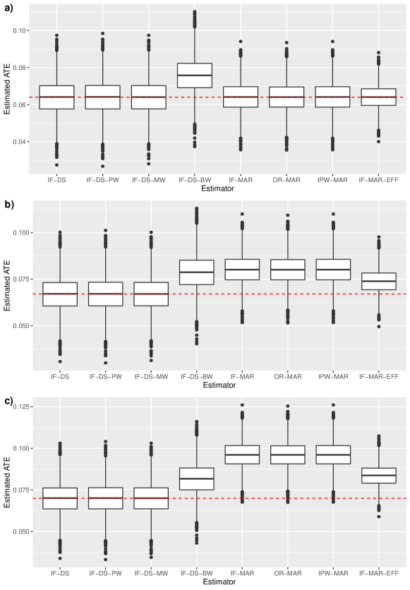
Figure 1: Simulation results for experiments of Section 4.1, with a) no violation of MAR ($\beta_{\_}{RA}=0$); b) a moderate violation of MAR ($\beta_{\_}{RA}=0.016$); and c) a large violation of MAR ($\beta_{\_}{RA}=0.032$). IF-DS = influence-function based estimator using double sampling, $\widehat{\tau}_{\_}1-\widehat{\tau}_{\_}0$; IF-DS-PW = IF-DS but with $\widehat{\pi}_{\_}a$ misspecified; IF-DS-MW = IF-DS but with $(\widehat{\mu}_{\_}{a,S},\widehat{\mu}_{\_}{a,R},\widehat{\gamma}_{\_}a)$ misspecified; IF-DS-BW = IF-DS but with both $(\widehat{\mu}_{\_}{a,S},\widehat{\mu}_{\_}{a,R},\widehat{\gamma}_{\_}a)$ and $\widehat{\pi}_{\_}a$ misspecified; IF-MAR = augmented IPW-based estimator assuming MAR, $\widehat{\xi}_{\_}1-\widehat{\xi}_{\_}0$; OR-MAR = outcome regression-based estimator assuming MAR; IPW-MAR = IPW-based estimator assuming MAR; IF-MAR-EFF = semiparametric efficient estimator under MAR, $\widehat{\tau}_{\_}1^{*}-\widehat{\tau}_{\_}0^{*}$. ATE = average treatment effect; the red dashed line indicates the true ATE.

The results of the simulation study are presented in Figure 1. The robustness of the influence-function based estimator $\widehat{\tau}_{\_}1-\widehat{\tau}_{\_}0$ is clearly seen, as unbiased inference was obtained in all scenarios when all models were correctly specified, or either $(\widehat{\mu}_{\_}{a,S},\widehat{\mu}_{\_}{a,R},\widehat{\gamma}_{\_}a)$ or $\widehat{\pi}_{\_}a$ was misspecified. When both were misspecified, some bias was observed in all three MAR violation scenarios. The initial-sample-only MAR-based estimators had slightly lower variance, but were substantially biased when there was even a moderate violation of MAR. The MAR-efficient estimator $\widehat{\tau}_{\_}1^{*}-\widehat{\tau}_{\_}0^{*}$, as expected, had the lowest variance of all estimators and was unbiased in the MAR scenario. When there was a moderate or large violation of MAR, $\widehat{\tau}_{\_}1^{*}-\widehat{\tau}_{\_}0^{*}$ was biased, though less so than the initial-sample-only MAR-based estimators.

4.2 Inference and assessment of adaptive estimator

Within the same simulation framework, we also assessed the performance of the adaptive estimator (analysis strategy #5), and evaluated proposed confidence intervals of all the estimators considered. For each value in a grid of MAR violation parameters $\beta_{\_}{RA}\in[0,0.04]$, we simulated 5,000 datasets exactly as in the previous section. In each case, we computed both $\widehat{\tau}_{\_}1-\widehat{\tau}_{\_}0$ and $\widehat{\tau}_{\_}1^{*}-\widehat{\tau}_{\_}0^{*}$, where all underlying nuisance models were correctly specified. Based on these, we then also computed the adaptive estimator $\widehat{\tau}_{\_}1^{\dagger}-\widehat{\tau}_{\_}0^{\dagger}$.

Lastly, to show that care is required when using the data to decide between $\widehat{\tau}_{\_}1-\widehat{\tau}_{\_}0$ and $\widehat{\tau}_{\_}1^{*}-\widehat{\tau}_{\_}0^{*}$, we contrasted $\widehat{\tau}_{\_}1^{\dagger}-\widehat{\tau}_{\_}0^{\dagger}$ to an ad hoc adaptive estimator (analysis strategy #4). For this, we first test the hypothesis that $\tau_{\_}a(P_{\_}o)=\tau_{\_}a^{*}(P_{\_}o)$ by assessing the magnitude of the difference $\widehat{\tau}_{\_}a-\widehat{\tau}_{\_}a^{*}$. Formally, under appropriate conditions, Theorem A.1 implies that $\sqrt{n}(\widehat{\tau}_{\_}a-\widehat{\tau}_{\_}a^{*})\xrightarrow[\mathrm{MAR}]{d}\mathcal{N}(0,Q)$, where $Q=\mathrm{Var}_{\_}{P_{\_}o}(\dot{\tau}_{\_}a(O;P_{\_}o))+\mathrm{Var}_{\_}{P_{\_}o}(\dot{\tau}_{\_}a^{*}(O;P_{\_}o))-2\cdot\mathrm{Cov}_{\_}{P_{\_}o}(\dot{\tau}_{\_}a(O;P_{\_}o),\dot{\tau}_{\_}a^{*}(O;P_{\_}o))$. An ad hoc adaptive estimator is simply to choose $\widehat{\tau}_{\_}a$ if we reject a test of MAR based on this result, i.e., if $\sqrt{n}\left|\widehat{\tau}_{\_}a-\widehat{\tau}_{\_}a^{*}\right|\big{/}\sqrt{\widehat{Q}}>z_{\_}{1-\alpha/2}$, and otherwise choose $\widehat{\tau}_{\_}a^{*}$ if we fail to reject. We computed this estimator across all simulation settings.

To evaluate confidence intervals, we again focused on the three parameter values $\beta_{\_}{RA}\in\{0,0.016,0.032\}$. In the 5,000 simulated datasets for each value, we constructed confidence intervals for the four estimators described above. For $\widehat{\tau}_{\_}1-\widehat{\tau}_{\_}0$ and $\widehat{\tau}_{\_}1^{*}-\widehat{\tau}_{\_}0^{*}$, we used influence function-based Wald-type confidence intervals. For $\widehat{\tau}_{\_}1^{\dagger}-\widehat{\tau}_{\_}0^{\dagger}$, we constructed confidence intervals based on Theorem 4 of Rothenhäusler (2020). For the ad hoc adaptive estimator, we used the Wald-type interval corresponding to the baseline estimator chosen according to the hypothesis test — a naive approach which we expect will lead to undercoverage.

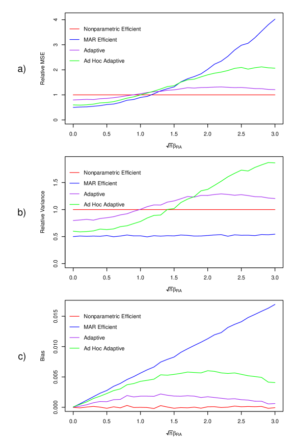
Figure 2: Simulation results for experiments of Section 4.2, regarding $\widehat{\tau}_{\_}1-\widehat{\tau}_{\_}0$, MAR semiparametric efficient estimator $\widehat{\tau}_{\_}1^{*}-\widehat{\tau}_{\_}0^{*}$, the adaptive estimator of Rothenhäusler (2020), $\widehat{\tau}_{\_}1^{\dagger}-\widehat{\tau}_{\_}0^{\dagger}$, and the ad hoc approach described in Section 4.1. Subplot a) shows the the empirical mean squared error (MSE) of each approach, divided by the MSE of the nonparametric efficient estimator. Subplot b) shows the empirical bias of each approach. Subplot c) shows the empirical variance of each approach, divided by the variance of the nonparametric efficient estimator.

The results on the grid of $\beta_{\_}{RA}$ values are shown in Figure 2. When $\beta_{\_}{RA}=0$ (i.e., MAR holds), all estimators are unbiased, $\widehat{\tau}_{\_}1^{*}-\widehat{\tau}_{\_}0^{*}$ is most efficient, and the two adaptive estimators have variance somewhere between that of $\widehat{\tau}_{\_}1^{*}-\widehat{\tau}_{\_}0^{*}$ and $\widehat{\tau}_{\_}1-\widehat{\tau}_{\_}0$. As $\beta_{\_}{RA}$ increases, the bias of $\widehat{\tau}_{\_}1^{*}-\widehat{\tau}_{\_}0^{*}$, which wrongly assumes MAR, increases roughly linearly. The two adaptive estimators also inherit some bias due to being pulled away by $\widehat{\tau}_{\_}1^{*}-\widehat{\tau}_{\_}0^{*}$. Interestingly, when $\beta_{\_}{RA}$ becomes really large, indicating quite a substantial violation of MAR, the bias of the two adaptive estimators returns back towards zero, as it becomes increasingly rare for either of these to select the estimator which assumes MAR.

The results on the focused set of values $\beta_{\_}{RA}\in\{0,0.016,0.032\}$ are arranged in Table 2. The confidence interval for $\widehat{\tau}_{\_}1-\widehat{\tau}_{\_}0$ has the appropriate coverage in all scenarios, as does the interval for $\widehat{\tau}_{\_}1^{*}-\widehat{\tau}_{\_}0^{*}$ when MAR holds. In the two MNAR settings, however, $\widehat{\tau}_{\_}1^{*}-\widehat{\tau}_{\_}0^{*}$ is biased and its confidence interval is off target. The confidence interval for the adaptive estimator $\widehat{\tau}_{\_}1^{\dagger}-\widehat{\tau}_{\_}0^{\dagger}$ also appears to be valid, with perhaps a bit of undercoverage in finite samples for moderately large values of $\beta_{\_}{RA}$. Finally, the naive confidence intervals of the ad hoc adaptive estimator tend to be overly narrow.

5 Data application

In this section, we present an analysis of the proposed methods to data from an EHR-based study comparing the effect of RYGB ($A=1$) versus VSG ($A=0$) bariatric surgery procedures on percent weight change at three years post-surgery ($Y$). Data were obtained from three health care sites within Kaiser Permanente: Northern California, Southern California, and Washington. Namely, in line with Arterburn et al. (2021), we use data on $n=13,514$ adult patients who underwent RYGB or VSG between January 2005 and September 2015, with complete weight data at baseline (closest measurement pre-surgery, up to 6 months) and follow-up (closest measurement within $\pm$ 90 days). See Table 3 for a summary of baseline characteristics. These data comprised the “complete-cases” from a larger collection of 30,991 patients for which follow-up outcomes were only partially observed.

We artificially imposed missingness in the outcome $Y$ on the complete-case data according to an MAR mechanism, as well as an MNAR mechanism. To construct a realistic MAR mechanism, we modeled the probability of missingness from the original larger collection of 30,991 patients using the following baseline covariates $\boldsymbol{L}$: baseline weight, health care site, year of surgery, age, gender, race/ethnicity, number of days of health care use in 7-12 month period pre-surgery, number of days hospitalized in pre-surgery year, smoking status, Charlson/Elixhauser comorbidity score, insurance type, clinical statuses for hypertension, coronary artery disease, diabetes, dyslipedemia, retinopathy, neuropathy, and mental health disorders, and use of medicines including, insulin, ACE inhibitors, ARB, statins, other lipid lowering medications, and other antihypertensives. We regressed the indicator for observing $Y$ on $A$ and $\boldsymbol{L}$ via a SuperLearner ensemble (with library $\{\texttt{SL.glm, SL.ranger, SL.rpart}\}$) using the corresponding R package (Polley et al., 2019). Next, to construct a MNAR mechanism, we augmented the fitted values $\widehat{\gamma}$ to include dependence on the outcome $Y$:

$$\widehat{\gamma}\ \longmapsto\ \mathrm{expit}\left\{\left(\mathrm{logit}(\widehat{\gamma})+\widetilde{Y}\left[0.7+0.8(1-A)-1.2\,\mathds{1}(\text{diabetes})+0.6\,\mathds{1}(\text{non-commercial insurance})\right]\right)\right\},$$

where $\widetilde{Y}$ is standardized BMI change at 3 years. Finally, these models were used to impose missing outcomes on the sample of $n=13,514$ patients by sampling $R$ according to a Bernoulli with probability given by the fitted values from the models. The resulting marginal probabilities of missingness were 26% and 28% in the MAR and MNAR settings, respectively.

In each of the missingness settings described above, we considered collecting a random subsample (i.e., those with $S=1$) of initially missing outcomes of size 500, 1,000, and 1,500. For each of the six resulting datasets, we computed and compared point estimates and 95% confidence intervals for analysis strategies #1, #2, #3, and #5. For analysis strategy #1, we targeted $\xi_{\_}1(P_{\_}o)-\xi_{\_}0(P_{\_}o)$, where $\xi_{\_}a(P_{\_}o)=\mathbb{E}_{\_}{P_{\_}o}(\mu_{\_}{a,R}(\boldsymbol{L}))$, with an augmented-IPW estimator as in Davidian et al. (2005) and Williamson et al. (2012). Analysis strategies #2, #3, and #5, correspond to estimators $\widehat{\tau}_{\_}1-\widehat{\tau}_{\_}0$, $\widehat{\tau}_{\_}1^{*}-\widehat{\tau}_{\_}0^{*}$, and $\widehat{\tau}_{\_}1^{\dagger}-\widehat{\tau}_{\_}0^{\dagger}$, respectively. As a benchmark, we compare to a standard full-data augmented-IPW estimator that uses outcome data from all $n=13,514$ patients. For all estimators, we used flexible SuperLearner ensembles for each component nuisance function, with a library of SL.glm, SL.ranger, and SL.rpart.

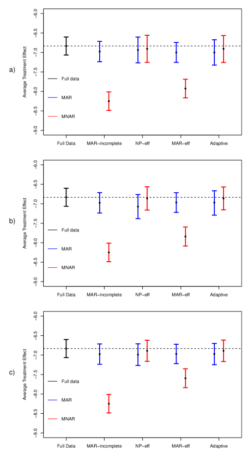
Figure 3: Results for data application in Section 5, showing the estimated effect on percent total weight change at 3 years. Subplots a), b), and c) correspond to follow-up subsamples of size 500, 1,000, and 1,500 individuals. Blue and red lines refer to estimated 95% confidence intervals when outcomes are initially MAR, and MNAR, respectively. Point estimates are marked with black dots. MAR-incomplete = augmented-IPW estimator with incomplete data only, assuming MAR; NP-eff = influence-function based estimator using double sampling, $\widehat{\tau}_{\_}1-\widehat{\tau}_{\_}0$; MAR-eff = semiparametric efficient estimator under MAR, $\widehat{\tau}_{\_}1^{*}-\widehat{\tau}_{\_}0^{*}$; Adaptive = adaptive estimator of Rothenhäusler (2020), $\widehat{\tau}_{\_}1^{\dagger}-\widehat{\tau}_{\_}0^{\dagger}$. The black dashed line represents the point estimate for the benchmark complete-case analysis.

Results are summarized in Figure 3. When MAR holds, all estimators perform well with respect to the benchmark analysis, with $\widehat{\tau}_{\_}1^{*}-\widehat{\tau}_{\_}0^{*}$ having smallest variance, as anticipated. On the other hand, the estimators that assume MAR appear to be biased under MNAR, while the nonparametric efficient estimator $\widehat{\tau}_{\_}1-\widehat{\tau}_{\_}0$ and adaptive estimator $\widehat{\tau}_{\_}1^{\dagger}-\widehat{\tau}_{\_}0^{\dagger}$ (which do not assume MAR) are robust to this violation of MAR. As expected, as the second stage subsample size increases, precision improves for analysis strategies #2, #3, and #5, which incorporate this data.

6 Double sampling for arbitrary coarsening

In this paper, we have focused on the specific causal problem outlined in Section 2. That said, the nonparametric identification and estimation results are entirely generic, and do not depend on either the data structure of the given problem nor the specific mean counterfactual estimand of interest. In Appendix A, we lay out the notation for arbitrary coarsening of a given full data structure and show that under a generalization of Assumptions 3.2 and 3.2, double sampling identifies the complete data distribution; derive a transformation of the full data nonparametric influence function of an arbitrary smooth functional that yields the observed data nonparametric influence function; construct influence function-based estimators using sample splitting; and characterize the asymptotic behavior of these estimators, including multiple robustness properties.

7 Discussion

In summary, this paper proposes a general framework for the use of double-sampling as a means to address potentially MNAR missing data, when scientific interest lies in estimating causal ATEs. Key to the framework is a suite of novel analysis strategies that exploit data arising from the double sampling scheme, coupled with identifying assumptions that guarantee the corresponding estimators to be asymptotically normal, efficient, and robust.

Table 1 emphasizes that each of the proposed estimators require Assumption 3.2 to hold. In any given applied setting, this assumption will need to be carefully evaluated. As indicated in Section 3.2, depending on the context, one practical issue is that selection by the double sampling scheme may not necessarily yield complete data. In such settings, investigators will need to work through the same thought experiments that one usually would for the standard MAR assumption (such as Assumption 3.2) to try to understand why some individuals engage and others do not. If it is felt that engagement remains dependent on outcome status (beyond what is explained by what is known about the design and covariates ($A$, $\boldsymbol{L}$)), then sensitivity analyses or alternative identification schemes may be necessary; this is an on-going area of our work.

A second practical issue is that, even if all those selected actually engage, the data that arises from the double-sampling scheme may be subject to error or recall bias (Haneuse et al., 2016). In some settings, the potential for recall bias may be mitigated through the design. In Koffman et al. (2021), for example, the outcome of interest was weight change at three years post-surgery, so the investigators timed the invitation to participants to coincide with the five-year anniversary. Additionally, following the same broad philosophy of this paper, one could directly learn about potential recall bias by including some participants for whom $R$ = 1 in the double-sampling scheme. This, in turn, would enable a comparison between information provided by the patient and what is available in the EHR. How best to do this and use the resulting information, though, are open questions.

Notwithstanding these practical issues and the fact that logistical or financial considerations may altogether preclude the use of double sampling in some settings, we believe the proposed framework presents a new option for researchers as they contend with potentially informative missing or coarsened data. Beyond those mentioned above, there are many opportunities for future work in this vein, including how best to use the available information in the EHR when allocating resources for double-sampling, as well as developing estimators for a broader set of analysis goals, such as mediation, and outcome types, such as time-to-event outcomes.

Table 1: Summary of Analysis Strategies #1–5

Strategy		Data		Assumptions		Estimator
#1		$(\boldsymbol{L},A,R,RY)$		(2.2)		Standard/ad-hoc
#2		$(\boldsymbol{L},A,R,S,(R+S)Y)$		(3.2) & (3.2)		IF-based, $\widehat{\tau}_{\_}a$
#3		$(\boldsymbol{L},A,R,S,(R+S)Y)$		(2.2) & (3.2)		IF-based, $\widehat{\tau}^{*}_{\_}a$
#4		$(\boldsymbol{L},A,R,S,(R+S)Y)$		(2.2) & (3.2) or (3.2) & (3.2)		$\widehat{\tau}_{\_}a$ or $\widehat{\tau}^{*}_{\_}a$
#5		$(\boldsymbol{L},A,R,S,(R+S)Y)$		(2.2) & (3.2) or (3.2) & (3.2)		$\widehat{\tau}_{\_}a^{\dagger}$

Table 2: Coverage and other statistics of influence function-based and adaptive estimators

% Bias Rel. variance Rel. MSE % Coverage Average length $\beta_{\_}{RA}=0$ $\widehat{\tau}_{\_}1-\widehat{\tau}_{\_}0$ -0.02 1.00 1.00 94.5 0.036 $\widehat{\tau}_{\_}1^{*}-\widehat{\tau}_{\_}0^{*}$ 0.06 0.50 0.50 95.4 0.026 $\widehat{\tau}_{\_}1^{\dagger}-\widehat{\tau}_{\_}0^{\dagger}$ 0.04 0.80 0.80 95.8 0.035 Ad hoc adaptive 0.08 0.64 0.64 93.8 0.026 $\beta_{\_}{RA}=0.016$ $\widehat{\tau}_{\_}1-\widehat{\tau}_{\_}0$ -0.01 1.00 1.00 94.5 0.036 $\widehat{\tau}_{\_}1^{*}-\widehat{\tau}_{\_}0^{*}$ 10.26 0.50 1.06 81.8 0.026 $\widehat{\tau}_{\_}1^{\dagger}-\widehat{\tau}_{\_}0^{\dagger}$ 2.87 1.08 1.12 94.1 0.036 Ad hoc adaptive 5.67 1.01 1.18 82.6 0.028 $\beta_{\_}{RA}=0.032$ $\widehat{\tau}_{\_}1-\widehat{\tau}_{\_}0$ -0.03 1.00 1.00 94.5 0.036 $\widehat{\tau}_{\_}1^{*}-\widehat{\tau}_{\_}0^{*}$ 19.57 0.51 2.72 45.3 0.026 $\widehat{\tau}_{\_}1^{\dagger}-\widehat{\tau}_{\_}0^{\dagger}$ 1.69 1.26 1.28 91.3 0.037 Ad hoc adaptive 4.56 1.56 1.68 73.6 0.031 • MSE, mean squared error; % Bias, $100\times\frac{\mathrm{mean}-(\tau_{\_}1(P_{\_}o)-\tau_{\_}0(P_{\_}o))}{\tau_{\_}1(P_{\_}o)-\tau_{\_}0(P_{\_}o)}$; Rel. variance, empirical variance of estimator divided by that of $\widehat{\tau}_{\_}1-\widehat{\tau}_{\_}0$; Rel. MSE, empirical MSE of estimator divided by that of $\widehat{\tau}_{\_}1-\widehat{\tau}_{\_}0$.

Table 3: Baseline characteristics of patients who underwent bariatric surgery, 2005–2015

	Surgery patients
Number	13514
Sleeve Gastrectomy [surgery type] (%)	4659 (34.5)
Health care site (%)
Washington	606 (4.5)
Northern California	3484 (25.8)
Southern California	9424 (69.7)
Year of surgery (mean (SD))	2009.64 (1.95)
Years of age at surgery (mean (SD))	46.29 (11.04)
Age categories (%)
1: $\mathrm{Age}<45$	5939 (43.9)
2: $45\leq\mathrm{Age}<65$	7019 (51.9)
3: $\mathrm{Age}\geq 65$	556 (4.1)
Male [gender] (%)	2233 (16.5)
Race/ethnicity (%)
Black	2471 (18.3)
Hispanic	4167 (30.8)
Unknown/Other	469 (3.5)
White	6407 (47.4)
Days of health care use 7-12 months pre-surgery (mean (SD))	9.24 (7.36)
Insulin use (%)	1651 (12.2)
Charlson/Elixhauser comorbidity score (%)
-1	2667 (19.7)
0	5147 (38.1)
1	3249 (24.0)
2	2451 (18.1)
Hypertension diagnosis (%)	8063 (59.7)
ACE inhibitor use (%)	3437 (25.4)
ARB use (%)	1199 (8.9)
Other antihypertensive medication (%)	5801 (42.9)
Insurance type (%)
Commercial	12096 (89.5)
Medicaid	488 (3.6)
Medicare	930 (6.9)
Diabetes status (%)	4956 (36.7)
Days hospitalized in year pre-surgery (mean (SD))	0.34 (1.81)
Dyslipidemia diagnosis (%)	6474 (47.9)
Statin use (%)	3667 (27.1)
Other lipid-lowering medication (%)	422 (3.1)
Smoking status (%)
Ever, Self-Report	4684 (34.7)
Never, Self-Report	7468 (55.3)
No Self-Report	1362 (10.1)
Coronary artery disease (%)	355 (2.6)
Mental health diagnoses (%)
Mild-Moderate Anxiety/Depression	5822 (43.1)
None	6096 (45.1)
Other	1596 (11.8)
Retinopathy (%)	615 ( 4.6)
Neuropathy (%)	945 ( 7.0)
Baseline BMI (mean (SD))	44.55 (7.12)

Appendix A General Coarsening Framework and Nonparametric Results

A.1 Coarsened data and nonparametric identification

Suppose the desired complete data for a given problem are the random vector $\boldsymbol{X}\sim P_{\_}{\boldsymbol{X}}^{*}$. That is, with $\boldsymbol{X}$ observed on every subject in a random sample, a parameter of interest, say $\chi(P_{\_}{\boldsymbol{X}}^{*})$, could be estimated consistently. Suppose, however, that the initially observed data consists only of $(C,\sigma_{\_}C(\boldsymbol{X}))$, where $C\in\mathbb{N}$ is a coarsening random variable, and $\sigma_{\_}C(\boldsymbol{X})$ is a coarsened version of the complete data: $\sigma_{\_}k$ is some (typically many-to-one) function for every possible value $k$ of $C$. As in Tsiatis (2007), we will write $C=\infty$ to denote that the complete data are observed, i.e., there is no coarsening. We will further assume that there exist functions $\overline{\sigma}_{\_}k$ for every $k$, such that $(\sigma_{\_}k,\overline{\sigma}_{\_}k)$ is injective; that is, there exist functions $h_{\_}k$ with $h_{\_}k(\sigma_{\_}k(\boldsymbol{X}),\overline{\sigma}_{\_}k(\boldsymbol{X}))=\boldsymbol{X}$. In our previous observational example from Section 2, $C=R\cdot\infty$, where $0\cdot\infty=0$, and $\sigma_{\_}0(\boldsymbol{X})=(\boldsymbol{L},A)$, $\overline{\sigma}_{\_}0(\boldsymbol{X})=Y$.

We now suppose that a subsample is intensively followed up, and the initially unobserved data $\overline{\sigma}_{\_}C(\boldsymbol{X})$ are obtained on some subjects. Let $S\in\{0,1\}$ indicate successful follow-up in the subsample when $S=1$. The full data are $(C,\sigma_{\_}C(\boldsymbol{X}),S,\overline{\sigma}_{\_}C(\boldsymbol{X}))\sim P^{*}$, and the final observed data are independent and identically distributed copies of $O=(C,\sigma_{\_}C(\boldsymbol{X}),S,S\cdot\overline{\sigma}_{\_}C(\boldsymbol{X}))\sim P$. Here, as before, the observed data probability distribution $P$ and the complete data distribution $P_{\_}{\boldsymbol{X}}^{*}$ are induced by $P^{*}$. Henceforth, we suppose that the data at hand are a random sample $O_{\_}1,\ldots,O_{\_}n\overset{\mathrm{iid}}{\sim}P$.

Let $p=\frac{dP}{d\mu}$ and $p^{*}=\frac{dP^{*}}{d\mu}$ denote the densities for $P$ and $P^{*}$, respectively, both with respect to some dominating measure $\mu$. The density of the full data distribution can be factored via $p^{*}(C,\sigma_{\_}C(\boldsymbol{X}),S,\overline{\sigma}_{\_}C(\boldsymbol{X}))=p(C,\sigma_{\_}C(\boldsymbol{X}),S)\times\prod_{\_}{k}p^{*}(\overline{\sigma}_{\_}k(\boldsymbol{X})\mid C=k,\sigma_{\_}k(\boldsymbol{X}),S)^{\mathds{1}(C=k)}$, whereas the density of the observed data can be factored via $p(O)=p(C,\sigma_{\_}C(\boldsymbol{X}),S)\times\prod_{\_}{k}p(\overline{\sigma}_{\_}k(\boldsymbol{X})\mid C=k,\sigma_{\_}k(\boldsymbol{X}),S=1)^{\mathds{1}(S=1,C=k)}$. As the conditioning event $S=0$ is possible in the full data but not in the observed data (i.e., appears in expression for $p^{*}$ but not for $p$), $P^{*}$ will not be identified from the observed data distribution $P$ unless further assumptions are made. That said, analysis of the components of the full data density $p^{*}$ that are not present in $p$ motivates the following conditions, which generalize Assumptions 3.2 and 3.2. [No informative second-stage selection, general version] For all $k\neq\infty$, $S\mathchoice{\mathrel{\hbox to0.0pt{$\displaystyle\perp$\hss}\mkern 2.0mu{\displaystyle\perp}}}{\mathrel{\hbox to0.0pt{$\textstyle\perp$\hss}\mkern 2.0mu{\textstyle\perp}}}{\mathrel{\hbox to0.0pt{$\scriptstyle\perp$\hss}\mkern 2.0mu{\scriptstyle\perp}}}{\mathrel{\hbox to0.0pt{$\scriptscriptstyle\perp$\hss}\mkern 2.0mu{\scriptscriptstyle\perp}}}\overline{\sigma}_{\_}k(\boldsymbol{X})\mid C=k,\sigma_{\_}k(\boldsymbol{X})$. [Positivity of second-stage sampling probabilities, general version] For some $\epsilon>0$, $P\left[P[S=1\mid C=k,\sigma_{\_}k(\boldsymbol{X})]\geq\epsilon\right]=1$, for all $k\neq\infty$. By the following result, a generalization of Proposition 1, Assumptions A.1 and A.1 are sufficient to identify the full data distribution $P^{*}$.

Proposition A.1

Assumptions A.1 and A.1 are sufficient to identify the full data distribution $P^{*}$ from the observed data distribution $P$.

Proof A.2

By Assumption A.1, the full data distribution may be factorized via

$$\begin{split}p^{*}(C,\sigma_{\_}C(\boldsymbol{X}),S,\overline{\sigma}_{\_}C(\boldsymbol{X}))&=p(C,\sigma_{\_}C(\boldsymbol{X}),S)p^{*}(\overline{\sigma}_{\_}C(\boldsymbol{X})\mid C,\sigma_{\_}C(\boldsymbol{X}),S)\\ &=p(C,\sigma_{\_}C(\boldsymbol{X}),S)p(\overline{\sigma}_{\_}C(\boldsymbol{X})\mid C,\sigma_{\_}C(\boldsymbol{X}),S=1)\end{split}$$ (2)

which only depends on the observed data distribution $p$. Note that we may safely introduce $S=1$ in the conditioning event due to Assumption A.1, and we may ignore the vacuous case $C=\infty$ as $\sigma_{\_}\infty(\boldsymbol{X})=\boldsymbol{X}$, given which $\overline{\sigma}_{\_}{\infty}(\boldsymbol{X})$ is degenerate.

The identifying Assumption A.1 may be interpreted as asserting that whether or not a subject is successfully double sampled is independent of all the initially unobserved data, conditional on all the initially observed data. While we have circumvented the need for the usual coarsening at random assumption for the initial sample, it is worth noting that given only observed data $O$, Assumption A.1 is untestable. In practice, however, these can be ensured by certain study designs and the successful follow-up of the chosen subsample: (i) subsample selection completely at random prior to the study; (ii) subsample selected at random among those with any initially missing information; and (iii) subsample selected with investigator-defined probabilities depending only on $(C,\sigma_{\_}C(\boldsymbol{X}))$. Of course, successful follow-up of the entire intended subsample may not be possible, and in these cases it must be that initially observed data is sufficient to predict successful follow-up. In general, if the same method of contacting subjects is used at the first stage and second stage of data collection, then it may be unreasonable to assume that coarsening at random fails to hold but Assumption A.1 is valid. Thus, the double sampling approach may be most justifiable when the method of data collection at the second stage differs from the first, e.g., in the EHR example, where the initial sample is the data that happened to be recorded in the electronic record, and the subsample is followed up via telephone or in-depth chart review.

On the other hand, Assumption A.1 asserts that there are no subpopulations, defined by observed data patterns, that are systematically excluded from the double sampling strategy (other than those with initially complete data) — if this were not the case, one could not learn about the subpopulations with initial missing information that were not followed up.

A.2 Estimation of complete data parameters

Suppose interest lies in estimating the complete data parameter $\chi(P_{\_}{\boldsymbol{X}}^{*})\in\mathbb{R}$, viewed as a functional from a model space of probability distributions on $\boldsymbol{X}$ — to which $P_{\_}{\boldsymbol{X}}^{*}$ belongs — to the real line. By Proposition A.1, under Assumptions A.1 and A.1, any complete data functional $\chi(P_{\_}{\boldsymbol{X}}^{*})$ has a corresponding observed data functional representation $\tau(P)$. For example, if $\chi(P_{\_}{\boldsymbol{X}}^{*})=\mathbb{E}_{\_}{P^{*}}(g(\boldsymbol{X}))$, for some function $g$, then $\chi(P_{\_}{\boldsymbol{X}}^{*})=\mathbb{E}_{\_}{P}(\mathbb{E}_{\_}{P^{*}}(g(\boldsymbol{X})\mid C,\sigma_{\_}C(\boldsymbol{X})))=\mathbb{E}_{\_}P(\mathbb{E}_{\_}{P}(g(\boldsymbol{X})\mid C,\sigma_{\_}C(\boldsymbol{X}),S=1))\eqqcolon\tau(P)$. It will often be the case that if the complete data $\boldsymbol{X}$ were completely observed, one would have in mind a valid estimator of $\chi(P_{\_}{\boldsymbol{X}}^{*})$. A natural goal is thus to develop a general procedure that can in a certain sense transform a complete-data estimator into one that uses only the observed data $O_{\_}1,\ldots,O_{\_}n$. The following proposition is the key semiparametric-theoretical result that will facilitate such a procedure. Note that it can be seen as a special case of the general theory developed in Robins et al. (1994).

Proposition A.3

Suppose $\chi$ is pathwise differentiable with respect to the complete data model at $P_{\_}{\boldsymbol{X}}^{*}$, with influence function $\dot{\chi}(\boldsymbol{X};P_{\_}{\boldsymbol{X}}^{*})$ (with respect to maximal tangent space), and that Assumptions A.1 and A.1 hold. Then $\tau(P)=\chi(P_{\_}{\boldsymbol{X}}^{*})$ is pathwise differentiable with influence function $\dot{\tau}(O;P)=\nu_{\_}C(\sigma_{\_}C(\boldsymbol{X}))+\frac{S}{\eta(C,\sigma_{\_}C(\boldsymbol{X}))}\left\{\dot{\chi}(\boldsymbol{X};P_{\_}{\boldsymbol{X}}^{*})-\nu_{\_}C(\sigma_{\_}C(\boldsymbol{X}))\right\}$ at $P$, where $\nu_{\_}C(\sigma_{\_}C(\boldsymbol{X}))=\mathbb{E}_{\_}P(\dot{\chi}(\boldsymbol{X};P_{\_}{\boldsymbol{X}}^{*})\mid C,\sigma_{\_}C(\boldsymbol{X}),S=1)$, and $\eta(C,\sigma_{\_}C(\boldsymbol{X}))=P[S=1\mid C,\sigma_{\_}C(\boldsymbol{X})]$. Recalling that $\sigma_{\_}{\infty}(\boldsymbol{X})=\boldsymbol{X}$, we allow for the possibility that $\eta(\infty,\boldsymbol{X})=0$, and define $\dot{\tau}(O;P)$ to equal $\nu_{\_}{\infty}(\boldsymbol{X})=\dot{\chi}(\boldsymbol{X};P_{\_}{\boldsymbol{X}}^{*})$ when $C=\infty$.

Proof A.4

Recall from Bickel et al. (1993) and Tsiatis (2007) that an influence function of a pathwise differentiable functional $\chi(P)$, at $P$ in a given statistical model, is a zero-mean finite-variance function $\dot{\chi}(O;P)$ of observed data $O$ such that for any regular parametric submodel $\{P_{\_}{\epsilon}:\epsilon\in[0,1)\}$ through $P_{\_}{0}\equiv P$, it holds that

$$\left.\frac{d}{d\epsilon}\chi(P_{\_}\epsilon)\right|_{\_}{\epsilon=0}=\mathbb{E}_{\_}P\left(\dot{\chi}(O;P)g(O)\right),$$

where $g(O)$ is the score function of the parametric submodel at $P$. The tangent set $\mathcal{T}_{\_}P$ of the statistical model at $P$ is the set of all score functions of one-dimensional regular parametric submodels through $P$, and the tangent space is $\Lambda_{\_}P=\overline{[\mathcal{T}_{\_}P]}$, the closure of the linear span (with respect to the Hilbert space $L_{\_}2(P)$) of the tangent set. The efficient influence function of $\chi$ at $P$ is the unique influence function belonging to $\Lambda_{\_}P$. When $\Lambda_{\_}P=L_{\_}2(P)$, the model is said to be nonparametric, and there is a unique influence function, often called the nonparametric influence function. See Bickel et al. (1993) and Van der Vaart (2000) for precise definitions.

Let $\{P_{\_}{\epsilon}\mid\epsilon\in[0,1)\}$ be an arbitrary one-parameter regular parametric submodel through $P\equiv P_{\_}0$. Note that, for any $\epsilon\in[0,1)$,

$$p_{\_}\epsilon(O)=p_{\_}\epsilon(C,\sigma_{\_}C(\boldsymbol{X}),S)p_{\_}\epsilon(\overline{\sigma}_{\_}C(\boldsymbol{X})\mid C,\sigma_{\_}C(\boldsymbol{X}),S=1)^{S},$$

so we must have

$$g(O)=g_{\_}{C,\sigma_{\_}C(\boldsymbol{X}),S}+S\cdot g_{\_}{\overline{\sigma}_{\_}C(\boldsymbol{X})\mid C,\sigma_{\_}C(\boldsymbol{X}),S=1},$$

where $g(O)$ is the score function of the submodel, typically

$$g(O)=\left.\frac{d}{d\epsilon}\log{(p_{\_}{\epsilon}(O))}\right|_{\_}{\epsilon=0},$$

and $g_{\_}{A\mid B}$ is the conditional score of $A$ given $B$ for arbitrary variables $A,B$. Of course, this submodel defines a regular parametric submodel $\{P_{\_}{\epsilon}^{*}\mid\epsilon\in[0,1)\}$ through the full data distribution $P^{*}\equiv P_{\_}{0}^{*}$ by Assumption A.1: for any $\epsilon\in[0,1)$,

$$p_{\_}{\epsilon}^{*}(C,\sigma_{\_}C(\boldsymbol{X}),S,\overline{\sigma}_{\_}C(\boldsymbol{X}))=p_{\_}\epsilon(C,\sigma_{\_}C(\boldsymbol{X}),S)p_{\_}\epsilon(\overline{\sigma}_{\_}C(\boldsymbol{X})\mid C,\sigma_{\_}C(\boldsymbol{X}),S=1).$$

Next, observe that

$$\mathbb{E}_{\_}P\left(\frac{S}{\eta(C,\sigma_{\_}C(\boldsymbol{X}))}\nu_{\_}C(\sigma_{\_}C(\boldsymbol{X}))g(O)\right)$$

$$=\mathbb{E}_{\_}P\left(\frac{S}{\eta(C,\sigma_{\_}C(\boldsymbol{X}))}\nu_{\_}C(\sigma_{\_}C(\boldsymbol{X}))g_{\_}{C,\sigma_{\_}C(\boldsymbol{X}),S}\right),$$

$$=\mathbb{E}_{\_}{P}\left(\frac{S}{\eta(C,\sigma_{\_}C(\boldsymbol{X}))}\dot{\chi}(\boldsymbol{X};P_{\_}{\boldsymbol{X}}^{*})g_{\_}{C,\sigma_{\_}C(\boldsymbol{X}),S}\right).$$

Here, the first equality results from conditioning on $(C,\sigma_{\_}C(\boldsymbol{X}),S)$, given which $g_{\_}{\overline{\sigma}_{\_}C(\boldsymbol{X})\mid C,\sigma_{\_}C(\boldsymbol{X}),S}$ has mean zero ($g_{\_}{\overline{\sigma}_{\_}C(\boldsymbol{X})\mid C,\sigma_{\_}C(\boldsymbol{X}),S=1}$ can be replaced by $g_{\_}{\overline{\sigma}_{\_}C(\boldsymbol{X})\mid C,\sigma_{\_}C(\boldsymbol{X}),S}$ due to the presence of indicator $S$). The second equality again can be seen by conditioning throughout by $(C,\sigma_{\_}C(\boldsymbol{X}),S)$. Thus,

$$\mathbb{E}_{\_}P\left(\frac{S}{\eta(C,\sigma_{\_}C(\boldsymbol{X}))}\left\{\dot{\chi}(\boldsymbol{X};P_{\_}{\boldsymbol{X}}^{*})-\nu_{\_}C(\sigma_{\_}C(\boldsymbol{X}))\right\}g(O)\right)$$

$$=\mathbb{E}_{\_}{P}\left(\frac{S}{\eta(C,\sigma_{\_}C(\boldsymbol{X}))}\dot{\chi}(\boldsymbol{X};P_{\_}{\boldsymbol{X}}^{*})[g(O)-g_{\_}{C,\sigma_{\_}C(\boldsymbol{X}),S}]\right),$$

$$=\mathbb{E}_{\_}{P}\left(\frac{S}{\eta(C,\sigma_{\_}C(\boldsymbol{X}))}\dot{\chi}(\boldsymbol{X};P_{\_}{\boldsymbol{X}}^{*})g_{\_}{\overline{\sigma}_{\_}C(\boldsymbol{X})\mid C,\sigma_{\_}C(\boldsymbol{X}),S=1}\right),\text{ since }S^{2}=S,$$

$$=\mathbb{E}_{\_}{P^{*}}\left(\frac{P^{*}[S=1\mid C,\sigma_{\_}C(\boldsymbol{X}),\overline{\sigma}_{\_}C(\boldsymbol{X})]}{\eta(C,\sigma_{\_}C(\boldsymbol{X}))}\dot{\chi}(\boldsymbol{X};P_{\_}{\boldsymbol{X}}^{*})g_{\_}{\overline{\sigma}_{\_}C(\boldsymbol{X})\mid C,\sigma_{\_}C(\boldsymbol{X}),S=1}\right),$$

$$=\mathbb{E}_{\_}{P^{*}}\left(\dot{\chi}(\boldsymbol{X};P_{\_}{\boldsymbol{X}}^{*})g_{\_}{\overline{\sigma}_{\_}C(\boldsymbol{X})\mid C,\sigma_{\_}C(\boldsymbol{X}),S=1}\right).$$

In the third equality, we introduced $P^{*}$ as it induces $P$, we conditioned on $(C,\sigma_{\_}C(\boldsymbol{X}),\overline{\sigma}_{\_}C(\boldsymbol{X}))$, and used the fact that, by construction, $\boldsymbol{X}$ is equal to $h_{\_}C(\sigma_{\_}C(\boldsymbol{X}),\overline{\sigma}_{\_}C(\boldsymbol{X}))$; in the fourth equality, we used Assumption A.1.

Now, see that

$$\mathbb{E}_{\_}P\left(\nu_{\_}C(\sigma_{\_}C(\boldsymbol{X}))g(O)\right) =\mathbb{E}_{\_}P\left(\nu_{\_}C(\sigma_{\_}C(\boldsymbol{X}))g_{\_}{C,\sigma_{\_}C(\boldsymbol{X}),S}\right),$$

$$=\mathbb{E}_{\_}{P^{*}}\left(\dot{\chi}(\boldsymbol{X};P_{\_}{\boldsymbol{X}}^{*})g_{\_}{C,\sigma_{\_}C(\boldsymbol{X}),S}\right),$$

where in the first equality we note that $S\cdot g_{\_}{\overline{\sigma}_{\_}C(\boldsymbol{X})\mid C,\sigma_{\_}C(\boldsymbol{X}),S=1}$ has mean zero given $(C,\sigma_{\_}C(\boldsymbol{X}),S)$, and the second equality can be seen by conditioning on $(C,\sigma_{\_}C(\boldsymbol{X}),S)$ and again using $S\mathchoice{\mathrel{\hbox to0.0pt{$\displaystyle\perp$\hss}\mkern 2.0mu{\displaystyle\perp}}}{\mathrel{\hbox to0.0pt{$\textstyle\perp$\hss}\mkern 2.0mu{\textstyle\perp}}}{\mathrel{\hbox to0.0pt{$\scriptstyle\perp$\hss}\mkern 2.0mu{\scriptstyle\perp}}}{\mathrel{\hbox to0.0pt{$\scriptscriptstyle\perp$\hss}\mkern 2.0mu{\scriptscriptstyle\perp}}}\overline{\sigma}_{\_}C(\boldsymbol{X})\mid C,\sigma_{\_}C(\boldsymbol{X})$ under $P^{*}$.

Finally, defining

$$\dot{\tau}(O;P)=\nu_{\_}C(\sigma_{\_}C(\boldsymbol{X}))+\frac{S}{\eta(C,\sigma_{\_}C(\boldsymbol{X}))}\left\{\dot{\chi}(\boldsymbol{X};P_{\_}{\boldsymbol{X}}^{*})-\nu_{\_}C(\sigma_{\_}C(\boldsymbol{X}))\right\},$$

we have shown that

$$\mathbb{E}_{\_}P\left(\dot{\tau}(O;P)g(O)\right)=\mathbb{E}_{\_}{P^{*}}\left(\dot{\chi}(\boldsymbol{X};P_{\_}{\boldsymbol{X}}^{*})g^{*}\right),$$

where $g^{*}=g_{\_}{C,\sigma_{\_}C(\boldsymbol{X}),S}+g_{\_}{\overline{\sigma}_{\_}C(\boldsymbol{X})\mid C,\sigma_{\_}C(\boldsymbol{X}),S=1}$ is the score of the full data submodel through $P^{*}$. But by assumption that $\chi$ is regular at $P_{\_}{\boldsymbol{X}}^{*}$,

$$\mathbb{E}_{\_}{P^{*}}\left(\dot{\chi}(\boldsymbol{X};P_{\_}{\boldsymbol{X}}^{*})g^{*}\right)=\left.\frac{d}{d\epsilon}\chi(P_{\_}{\boldsymbol{X},\epsilon}^{*})\right|_{\_}{\epsilon=0},$$

so that

$$\left.\frac{d}{d\epsilon}\tau(P_{\_}{\epsilon})\right|_{\_}{\epsilon=0}=\mathbb{E}_{\_}P\left(\dot{\tau}(O;P)g(O)\right)$$

as $\tau(P_{\_}{\epsilon})=\chi(P_{\_}{\boldsymbol{X},\epsilon}^{*})$ for all $\epsilon\in[0,1)$, by construction. By definition, this means that $\dot{\tau}(O;P)$ is an influence function for $\tau$ at $P$, as claimed.

We remark that another way to interpret the term $\frac{S}{\eta(C,\sigma_{\_}C(\boldsymbol{X}))}$ in the case that $\eta(\infty,\boldsymbol{X})=0$ is to use the convention $0\cdot\infty=0$, so that the second term drops out.

We are now equipped to define a one-step estimator of the general functional $\tau(P)$ that uses its estimated influence function to correct the bias of a plugin estimator $\tau(\widehat{P})$. Depending on the form of the parameter and its influence function, certain components of the observed data distribution may not need to be estimated (e.g., the running causal example of this paper). In general, though, an estimate of $P_{\_}{\boldsymbol{X}}^{*}$ can be reconstructed by marginalizing an estimated version of the identified full data density (2) over $(C,S)$. Letting $\lambda_{\_}C(\overline{\sigma}_{\_}C(\boldsymbol{X});\sigma_{\_}C(\boldsymbol{X}))$ be the distribution function of $\overline{\sigma}_{\_}C(\boldsymbol{X})$ given $C,\sigma_{\_}C(\boldsymbol{X}),S=1$, we can use $\widehat{P}_{\_}{\boldsymbol{X}}^{*}$, $\widehat{\eta}$, $\widehat{\lambda}$ to obtain $\dot{\tau}(O;\widehat{P})=\widehat{\nu}_{\_}C(\sigma_{\_}C(\boldsymbol{X}))+\frac{S}{\widehat{\eta}(C,\sigma_{\_}C(\boldsymbol{X}))}\left\{\dot{\chi}(\boldsymbol{X};\widehat{P}_{\_}{\boldsymbol{X}}^{*})-\widehat{\nu}_{\_}C(\sigma_{\_}C(\boldsymbol{X}))\right\}$, where $\widehat{\nu}_{\_}C(\sigma_{\_}C(\boldsymbol{X}))=\int\dot{\chi}(h_{\_}C(\sigma_{\_}C(\boldsymbol{X}),\boldsymbol{t});\widehat{P}_{\_}{\boldsymbol{X}}^{*})\,d\widehat{\lambda}_{\_}{C}(\boldsymbol{t};\sigma_{\_}C(\boldsymbol{X}))$.

We propose to use sample splitting and cross-fitting (Chernozhukov et al., 2018), and fit $\widehat{P}_{\_}k$ using data $I_{\_}k^{c}$, for $k=1,\ldots,K$. We then define $\widehat{\tau}_{\_}k=\tau(\widehat{P}_{\_}k)+\frac{K}{n}\sum_{\_}{i\in I_{\_}k}\dot{\tau}(O_{\_}i;\widehat{P}_{\_}k),\text{ for }k=1,\ldots,K$, so that the sample-split influence function-based estimator is given by $\widehat{\tau}=\frac{1}{K}\sum_{\_}{k=1}^{k}\widehat{\tau}_{\_}k$.

A.3 Consistency, asymptotic normality, and robustness

The following result is the basis for consistency, asymptotic normality, nonparametric efficiency, and multiple robustness of the proposed nonparametric influence function-based estimator $\widehat{\tau}$.

Theorem A.5

Suppose $\left\lVert\dot{\tau}(\,\cdot\,;\widehat{P}_{\_}k)-\dot{\tau}(\,\cdot\,;P)\right\rVert=o_{\_}P(1)$ for $k=1,\ldots,K$. Then

$$\widehat{\tau}-\tau(P)=O_{\_}P\left(\frac{1}{\sqrt{n}}+\frac{1}{K}\sum_{\_}{k=1}^{K}\mathrm{Bias}_{\_}{\tau}(\widehat{P}_{\_}k;P)\right),$$

where $\mathrm{Bias}_{\_}{\tau}(\widehat{P};P)=\mathbb{E}_{\_}P(\dot{\tau}(O;\widehat{P}))+\tau(\widehat{P})-\tau(P)$ for any $\widehat{P}$. Moreover, if $\mathrm{Bias}_{\_}{\tau}(\widehat{P}_{\_}k;P)=o_{\_}P(n^{-1/2})$, for $k=1,\ldots,K$, then $\sqrt{n}(\widehat{\tau}-\tau(P))\overset{d}{\to}\mathcal{N}(0,V)$, where $V=\mathrm{Var}_{\_}P(\dot{\tau}(O;P))$ is the nonparametric efficiency bound.

Proof A.6

For a given subset $k\in\{1,\ldots,K\}$, we can decompose the error of $\widehat{\tau}_{\_}k$ relative to $\tau(P)$ via:

$$\widehat{\tau}_{\_}k-\tau(P) =\frac{K}{n}\sum_{\_}{i\in I_{\_}k}\dot{\tau}(O_{\_}i,P)$$

$$\quad\quad+\left\{\mathbb{E}_{\_}P(\dot{\tau}(O;\widehat{P}_{\_}k))+\tau(\widehat{P}_{\_}k)-\tau(P)\right\}$$

$$\quad\quad+\left\{\frac{K}{n}\sum_{\_}{i\in I_{\_}k}\left[\dot{\tau}(O_{\_}i;\widehat{P}_{\_}k)-\dot{\tau}(O_{\_}i,P)\right]-\mathbb{E}_{\_}P(\dot{\tau}(O;\widehat{P}_{\_}k))\right\}.$$

Thus, the error of $\widehat{\tau}$ with respect to $\tau(P)$ can be decomposed as follows:

$$\widehat{\tau}-\tau(P) =\frac{1}{n}\sum_{\_}{i=1}^{n}\dot{\tau}(O_{\_}i,P)+\frac{1}{K}\sum_{\_}{k=1}^{K}\mathrm{Bias}_{\_}{\tau}(\widehat{P}_{\_}k;P)$$

$$\quad\quad+\frac{1}{K}\sum_{\_}{k=1}^{K}\left\{\frac{K}{n}\sum_{\_}{i\in I_{\_}k}\left[\dot{\tau}(O_{\_}i;\widehat{P}_{\_}k)-\dot{\tau}(O_{\_}i,P)\right]-\mathbb{E}_{\_}P(\dot{\tau}(O;\widehat{P}_{\_}k))\right\}.$$

By the central limit theorem, the first term is $O_{\_}P(n^{-1/2})$ as

$$\frac{1}{\sqrt{n}}\sum_{\_}{i=1}^{n}\dot{\tau}(O_{\_}i,P)\overset{d}{\to}\mathcal{N}(0,V),$$

where $V=\mathrm{Var}_{\_}P(\dot{\tau}(O;P))$. Next, invoking Lemma 2 in Kennedy et al. (2020) or Kennedy (2020), for each $k=1,\ldots,K$, as $\{O_{\_}i:i\in I_{\_}k\}\mathchoice{\mathrel{\hbox to0.0pt{$\displaystyle\perp$\hss}\mkern 2.0mu{\displaystyle\perp}}}{\mathrel{\hbox to0.0pt{$\textstyle\perp$\hss}\mkern 2.0mu{\textstyle\perp}}}{\mathrel{\hbox to0.0pt{$\scriptstyle\perp$\hss}\mkern 2.0mu{\scriptstyle\perp}}}{\mathrel{\hbox to0.0pt{$\scriptscriptstyle\perp$\hss}\mkern 2.0mu{\scriptscriptstyle\perp}}}\{O_{\_}i:i\in I_{\_}k^{c}\}$,

$$\frac{K}{n}\sum_{\_}{i\in I_{\_}k}\left[\dot{\tau}(O_{\_}i;\widehat{P}_{\_}k)-\dot{\tau}(O_{\_}i,P)\right]-\mathbb{E}_{\_}P(\dot{\tau}(O;\widehat{P}_{\_}k))$$

$$=O_{\_}P\left(\frac{\sqrt{K}}{\sqrt{n}}\left\lVert\dot{\tau}(\,\cdot\,;\widehat{P}_{\_}k)-\dot{\tau}(\,\cdot\,;P)\right\rVert\right),$$

$$=o_{\_}P\left(\frac{\sqrt{K}}{\sqrt{n}}\right),$$

as $n/K\to\infty$, since $\left\lVert\dot{\tau}(\,\cdot\,;\widehat{P}_{\_}k)-\dot{\tau}(\,\cdot\,;P)\right\rVert=o_{\_}P(1)$ by assumption. Equivalently, as $n\to\infty$, this $k$-th term is $o_{\_}P(n^{-1/2})$. As $K$ is fixed, an average of $K$ such terms is also $o_{\_}P(n^{-1/2})$, and the result follows.

It is important to note that we have only established that $\widehat{\tau}$ is fully (semiparametric) efficient in a nonparametric model, i.e., when the model tangent space (see Bickel et al. (1993), Tsiatis (2007)) is $L_{\_}2^{0}(P)$, consisting of all mean-zero functions of $O$ with finite variance. Nonparametric efficiency of $\widehat{\tau}$ is guaranteed because there is a unique (thus efficient) influence function in a nonparametric model, its variance equal to the nonparametric efficiency bound (Bickel et al., 1993). Derivation of the semiparametric efficient observed data influence function in proper semiparametric models where restrictions are placed on $P$ will depend on the form of those restrictions (e.g., when MAR holds as in Analysis #3), so we leave characterizations of efficiency over classes of restrictions on $P$ for future research.

The next two propositions relate the asymptotic variance and bias term (as defined in Proposition A.3) of $\widehat{\tau}$ to that of a complete-data influence function based estimator.

Proposition A.7

Let $\dot{\tau}(O;P)$ be the observed data influence function defined in Proposition A.3, where $P$ is induced by $P^{*}$ satisfying Assumptions A.1 and A.1. Then the observed data nonparametric efficiency bound for estimating $\tau(P)=\chi(P_{\_}{\boldsymbol{X}}^{*})$ is given by: $\mathrm{Var}_{\_}P(\dot{\tau}(O;P))=\mathrm{Var}_{\_}{P^{*}}(\dot{\chi}(\boldsymbol{X};P_{\_}{\boldsymbol{X}}^{*}))+\mathbb{E}_{\_}P\left(\left(\frac{1}{\eta(C,\sigma_{\_}C(\boldsymbol{X}))}-1\right)\mathrm{Var}_{\_}P(\dot{\chi}(\boldsymbol{X};P_{\_}{\boldsymbol{X}}^{*})\mid C,\sigma_{\_}C(\boldsymbol{X}),S=1)\right)$.

Proof A.8

Note that the second summand of the observed data influence function $\dot{\tau}(O;P)$ has mean zero given $(C,\sigma_{\_}C(X),S)$, as

$$S\,\mathbb{E}_{\_}P\left(\dot{\chi}(\boldsymbol{X};P_{\_}{\boldsymbol{X}}^{*})-\nu_{\_}C(\sigma_{\_}C(\boldsymbol{X}))\,\middle|\,C,\sigma_{\_}C(X),S\right)$$

$$=S\left\{\mathbb{E}_{\_}P\left(\dot{\chi}(\boldsymbol{X};P_{\_}{\boldsymbol{X}}^{*})\,\middle|\,C,\sigma_{\_}C(\boldsymbol{X}),S=1\right)-\nu_{\_}C(\sigma_{\_}C(\boldsymbol{X}))\right\}$$

$$=0,$$

by definition of $\nu_{\_}C(\sigma_{\_}C(\boldsymbol{X}))$. It follows that the two summands are uncorrelated, and

$$\mathrm{Var}_{\_}P(\dot{\tau}(O;P)) =\mathrm{Var}_{\_}P(\nu_{\_}C(\sigma_{\_}C(\boldsymbol{X})))$$

$$\quad\quad+\mathrm{Var}_{\_}P\left(\frac{S}{\eta(C,\sigma_{\_}C(\boldsymbol{X}))}\left\{\dot{\chi}(\boldsymbol{X};P_{\_}{\boldsymbol{X}}^{*})-\nu_{\_}C(\sigma_{\_}C(\boldsymbol{X}))\right\}\right).$$

By the law of total variance, and given that the second summand has mean zero given $(C,\sigma_{\_}C(X),S)$,

$$\mathrm{Var}_{\_}P\left(\frac{S}{\eta(C,\sigma_{\_}C(\boldsymbol{X}))}\left\{\dot{\chi}(\boldsymbol{X};P_{\_}{\boldsymbol{X}}^{*})-\nu_{\_}C(\sigma_{\_}C(\boldsymbol{X}))\right\}\right)$$

$$=\mathbb{E}_{\_}P\left(\frac{S}{\eta(C,\sigma_{\_}C(\boldsymbol{X}))^{2}}\mathrm{Var}_{\_}P\left(\dot{\chi}(\boldsymbol{X};P_{\_}{\boldsymbol{X}}^{*})\mid C,\sigma_{\_}C(X),S=1\right)\right)$$

$$=\mathbb{E}_{\_}P\left(\frac{1}{\eta(C,\sigma_{\_}C(\boldsymbol{X}))}\mathrm{Var}_{\_}P\left(\dot{\chi}(\boldsymbol{X};P_{\_}{\boldsymbol{X}}^{*})\mid C,\sigma_{\_}C(X),S=1\right)\right),$$

where in the last equality we conditioned on $(C,\sigma_{\_}C(\boldsymbol{X}))$. Finally, as

$$\mathrm{Var}_{\_}P\left(\dot{\chi}(\boldsymbol{X};P_{\_}{\boldsymbol{X}}^{*})\mid C,\sigma_{\_}C(X),S=1\right)=\mathrm{Var}_{\_}{P^{*}}\left(\dot{\chi}(\boldsymbol{X};P_{\_}{\boldsymbol{X}}^{*})\mid C,\sigma_{\_}C(X)\right),$$

and

$$\mathbb{E}_{\_}P\left(\dot{\chi}(\boldsymbol{X};P_{\_}{\boldsymbol{X}}^{*})\,\middle|\,C,\sigma_{\_}C(\boldsymbol{X}),S=1\right)=\mathbb{E}_{\_}{P^{*}}\left(\dot{\chi}(\boldsymbol{X};P_{\_}{\boldsymbol{X}}^{*})\,\middle|\,C,\sigma_{\_}C(\boldsymbol{X})\right),$$

by Assumption A.1, adding and subtracting

$$\mathbb{E}_{\_}P\left(\mathrm{Var}_{\_}P\left(\dot{\chi}(\boldsymbol{X};P_{\_}{\boldsymbol{X}}^{*})\mid C,\sigma_{\_}C(X),S=1\right)\right)$$

yields the result, again by the law of total variance.

Proposition A.9

Let $P$, $\widetilde{P}$ be arbitrary putative observed data distributions, induced by full data distributions $P^{*}$, $\widetilde{P}^{*}$, respectively, and assume that both $P^{*}$ and $\widetilde{P}^{*}$ satisfy Assumptions A.1 and A.1. Then $\mathrm{Bias}_{\_}{\tau}(\widetilde{P};P)\coloneqq\mathbb{E}_{\_}P(\dot{\tau}(O;\widetilde{P}))+\tau(\widetilde{P})-\tau(P)$ is equal to $\mathrm{Bias}_{\_}{\chi}(\widetilde{P}_{\_}{\boldsymbol{X}}^{*};P_{\_}{\boldsymbol{X}}^{*})+\mathbb{E}_{\_}{P}\left[\left(1-\frac{\eta(C,\sigma_{\_}C(\boldsymbol{X}))}{\widetilde{\eta}(C,\sigma_{\_}C(\boldsymbol{X}))}\right)\left\{\widetilde{\nu}_{\_}C(\sigma_{\_}C(\boldsymbol{X}))-\check{\nu}_{\_}C(\sigma_{\_}C(\boldsymbol{X}))\right\}\right]$, where $\mathrm{Bias}_{\_}{\chi}(\widetilde{P}_{\_}{\boldsymbol{X}}^{*};P_{\_}{\boldsymbol{X}}^{*})$ is similarly defined to equal $\mathbb{E}_{\_}{P^{*}}(\dot{\chi}(\boldsymbol{X};\widetilde{P}_{\_}{\boldsymbol{X}}^{*}))+\chi(\widetilde{P}_{\_}{\boldsymbol{X}}^{*})-\chi(P_{\_}{\boldsymbol{X}}^{*})$, $\widetilde{\nu}_{\_}C(\sigma_{\_}C(\boldsymbol{X}))\coloneqq\mathbb{E}_{\_}{\widetilde{P}}(\dot{\chi}(\boldsymbol{X};\widetilde{P}_{\_}{\boldsymbol{X}}^{*})\mid C,\sigma_{\_}C(\boldsymbol{X}),S=1)$, and $\check{\nu}_{\_}C(\sigma_{\_}C(\boldsymbol{X}))\coloneqq\mathbb{E}_{\_}P(\dot{\chi}(\boldsymbol{X};\widetilde{P}_{\_}{\boldsymbol{X}}^{*})\mid C,\sigma_{\_}C(\boldsymbol{X}),S=1)$.

Proof A.10

Observe that

$$\mathbb{E}_{\_}P\left(\check{\nu}_{\_}C(\sigma_{\_}C(\boldsymbol{X}))\right)=\mathbb{E}_{\_}{P^{*}}(\dot{\chi}(\boldsymbol{X};\widetilde{P}_{\_}{\boldsymbol{X}}^{*})),$$

by iterated expectations and Assumption A.1. Moreover,

$$\mathbb{E}_{\_}P\left(\frac{S}{\widetilde{\eta}(C,\sigma_{\_}C(\boldsymbol{X}))}\left\{\dot{\chi}(\boldsymbol{X};\widetilde{P}_{\_}{\boldsymbol{X}}^{*})-\widetilde{\nu}_{\_}C(\sigma_{\_}C(\boldsymbol{X}))\right\}\right)$$

$$=\mathbb{E}_{\_}{P^{*}}\left(\frac{\eta(C,\sigma_{\_}C(\boldsymbol{X}))}{\widetilde{\eta}(C,\sigma_{\_}C(\boldsymbol{X}))}\left\{\dot{\chi}(\boldsymbol{X};\widetilde{P}_{\_}{\boldsymbol{X}}^{*})-\widetilde{\nu}_{\_}C(\sigma_{\_}C(\boldsymbol{X}))\right\}\right),$$

$$=\mathbb{E}_{\_}{P}\left(\frac{\eta(C,\sigma_{\_}C(\boldsymbol{X}))}{\widetilde{\eta}(C,\sigma_{\_}C(\boldsymbol{X}))}\left\{\check{\nu}_{\_}C(\sigma_{\_}C(\boldsymbol{X}))-\widetilde{\nu}_{\_}C(\sigma_{\_}C(\boldsymbol{X}))\right\}\right),$$

where in the first equality we condition on $(C,\sigma_{\_}C(\boldsymbol{X}),\overline{\sigma}_{\_}C(\boldsymbol{X}))$, and in the second equality we condition on $(C,\sigma_{\_}C(\boldsymbol{X}))$ and use Assumption A.1. Hence,

$$\mathbb{E}_{\_}P(\dot{\tau}(O;\widetilde{P}))$$

$$=\mathbb{E}_{\_}P\left(\widetilde{\nu}_{\_}C(\sigma_{\_}C(\boldsymbol{X}))+\frac{S}{\widetilde{\eta}(C,\sigma_{\_}C(\boldsymbol{X}))}\left\{\dot{\chi}(\boldsymbol{X};\widetilde{P}_{\_}{\boldsymbol{X}}^{*})-\widetilde{\nu}_{\_}C(\sigma_{\_}C(\boldsymbol{X}))\right\}\right),$$

$$=\mathbb{E}_{\_}P\left(\check{\nu}_{\_}C(\sigma_{\_}C(\boldsymbol{X}))\right)+\mathbb{E}_{\_}P\left(\widetilde{\nu}_{\_}C(\sigma_{\_}C(\boldsymbol{X}))-\check{\nu}_{\_}C(\sigma_{\_}C(\boldsymbol{X}))\right)$$

$$\quad\quad+\mathbb{E}_{\_}{P}\left(\frac{\eta(C,\sigma_{\_}C(\boldsymbol{X}))}{\widetilde{\eta}(C,\sigma_{\_}C(\boldsymbol{X}))}\left\{\check{\nu}_{\_}C(\sigma_{\_}C(\boldsymbol{X}))-\widetilde{\nu}_{\_}C(\sigma_{\_}C(\boldsymbol{X}))\right\}\right),$$

$$=\mathbb{E}_{\_}{P^{*}}(\dot{\chi}(\boldsymbol{X};\widetilde{P}_{\_}{\boldsymbol{X}}^{*}))$$

$$\quad\quad+\mathbb{E}_{\_}{P}\left[\left(1-\frac{\eta(C,\sigma_{\_}C(\boldsymbol{X}))}{\widetilde{\eta}(C,\sigma_{\_}C(\boldsymbol{X}))}\right)\left\{\widetilde{\nu}_{\_}C(\sigma_{\_}C(\boldsymbol{X}))-\check{\nu}_{\_}C(\sigma_{\_}C(\boldsymbol{X}))\right\}\right].$$

The result is obtained by noticing that $\chi(P_{\_}{\boldsymbol{X}}^{*})=\tau(P)$, $\chi(\widetilde{P}_{\_}{\boldsymbol{X}}^{*})=\tau(\widetilde{P})$.

Remark A.11

By Proposition A.9, we expect the observed-data influence function-based estimator $\widehat{\tau}$ to at least partially inherit robustness properties of the complete data influence function-based estimator $\widehat{\chi}$. The second term in the bias expression can be rewritten

$$\mathbb{E}_{\_}{P^{*}}\left[\left(1-\frac{\eta(C,\sigma_{\_}C(\boldsymbol{X}))}{\widetilde{\eta}(C,\sigma_{\_}C(\boldsymbol{X}))}\right)\left(\frac{\widetilde{\lambda}_{\_}{C}^{\prime}(\overline{\sigma}_{\_}C(\boldsymbol{X});\sigma_{\_}C(\boldsymbol{X}))}{\lambda_{\_}{C}^{\prime}(\overline{\sigma}_{\_}C(\boldsymbol{X});\sigma_{\_}C(\boldsymbol{X}))}-1\right)\dot{\chi}(\boldsymbol{X};\widetilde{P}_{\_}{\boldsymbol{X}}^{*})\right],$$ (3)

where $\lambda_{\_}k^{\prime}$, $\widetilde{\lambda}_{\_}k^{\prime}$ are conditional densities of $\overline{\sigma}_{\_}k(\boldsymbol{X})$ given $C=k,\sigma_{\_}k(\boldsymbol{X}),S=1$ under $P$ and $\widetilde{P}$, respectively, for any $k\neq\infty$. This term can be simplified in certain examples (e.g., in our running example), but generally also exhibits a double robust property: it is zero if either $\widetilde{\eta}=\eta$ or $\widetilde{\lambda}=\lambda$. Thus, when the double sampling probabilities $\eta(C,\sigma_{\_}{C}(\boldsymbol{X}))$ are known by design, this term is automatically zero, so that $\mathrm{Bias}_{\_}{\tau}(\widetilde{P};P)=\mathrm{Bias}_{\_}{\chi}(\widetilde{P}_{\_}{\boldsymbol{X}}^{*};P_{\_}{\boldsymbol{X}}^{*})$.

The variance formula of Proposition A.7 facilitates an analysis of the loss of efficiency that the estimator based on double sampling incurs, compared to a complete-data influence function-based estimator that uses $\boldsymbol{X}$ on the complete sample. On the other hand, in view of Theorem A.5, the bias formula in Proposition A.9 is essential for determining conditions under which $\widehat{\tau}$ will be asymptotically normal and with variance attaining the nonparametric efficiency bound.

To elaborate on the previous point, for many common functionals (e.g., the running example in Section 2), the complete data asymptotic bias term $\mathrm{Bias}_{\_}{\chi}(\widehat{P}_{\_}{\boldsymbol{X}}^{*};P_{\_}{\boldsymbol{X}}^{*})$ exhibits a “mixed bias” property (Robins et al., 2008; Rotnitzky et al., 2020), in that it involves the product of nuisance function estimation errors. Moreover, the additional term in the bias expression also has this property: it is zero if either $\widehat{\eta}=\eta$ or $\widehat{\lambda}_{\_}k=\lambda_{\_}k$ for all $k\neq\infty$. In particular, this additional term is guaranteed to be zero when the double sampling probabilities $\eta$ are known by design. Thus, the proposed observed data influence function-based estimators inherit any robustness properties of their complete data counterparts when $\eta$ is known, and otherwise will have a slightly more elaborate multiple robustness structure due to the additional term.

Another important consequence of the mixed bias property is that of “rate double robustness” (Rotnitzky et al., 2020). Specifically, in the complete data setting, if $\mathrm{Bias}_{\_}{\chi}(\widehat{P}_{\_}{\boldsymbol{X}}^{*};P_{\_}{\boldsymbol{X}}^{*})$ depends on the product of $L_{\_}2(P)$-norm errors for estimating a pair of nuisance functions, and if this product converges to zero at rate $n^{-1/2}$, then the complete data influence function-based estimator will achieve $n^{-1/2}$ rate inference. The benefit is that this allows for more flexible estimation (e.g., errors converging faster than $n^{-1/4}$) of each of the nuisance functions, and the required convergence rates can be achieved by state-of-the-art machine learning models under smoothness or sparsity conditions, for example. In our case, we require the additional property that either $\eta$ is known, or else $\lVert\widehat{\eta}-\eta\rVert\lVert\widehat{\lambda^{\prime}}/\lambda^{\prime}-1\rVert=o_{\_}P(n^{-1/2})$, where $\lambda^{\prime}$ is the density corresponding to $\lambda$.

Finally, by the asymptotic normality result of Theorem A.5, a simple asymptotic variance estimator can obtained from the empirical variance of the estimated influence functions. The variance estimate for general functional $\tau(P)$ is $n\cdot\widehat{\mathrm{Var}}(\widehat{\tau})=\frac{1}{n}\sum_{\_}{k=1}^{K}\sum_{\_}{i\in I_{\_}k}(\dot{\tau}(O_{\_}i;\widehat{P}_{\_}k))^{2}$. Further, a Wald-type confidence interval is given by $\widehat{\tau}\pm z_{\_}{1-\alpha/2}\sqrt{\widehat{\mathrm{Var}}(\widehat{\tau})},$ with $z_{\_}{\alpha}$ denoting the $\alpha$-quantile of the standard normal distribution.

Appendix B Semiparametric results under Assumption 2.2

The observed data density is given by

$$p_{\_}o(O)=p_{\_}o(\boldsymbol{L},A,R)p_{\_}o(Y\mid\boldsymbol{L},A,R=1)^{R}p_{\_}o(S\mid\boldsymbol{L},A,R=0)^{1-R}p_{\_}o(Y\mid\boldsymbol{L},A,S=1)^{S},$$

by Assumption 3.2 and the assertion that $R=1$ implies $S=0$, i.e., $S\equiv S(1-R)$. Under the MAR assumption (i.e., Assumption 2.2, $R\mathchoice{\mathrel{\hbox to0.0pt{$\displaystyle\perp$\hss}\mkern 2.0mu{\displaystyle\perp}}}{\mathrel{\hbox to0.0pt{$\textstyle\perp$\hss}\mkern 2.0mu{\textstyle\perp}}}{\mathrel{\hbox to0.0pt{$\scriptstyle\perp$\hss}\mkern 2.0mu{\scriptstyle\perp}}}{\mathrel{\hbox to0.0pt{$\scriptscriptstyle\perp$\hss}\mkern 2.0mu{\scriptscriptstyle\perp}}}Y\mid\boldsymbol{L},A$), and Assumption 3.2, $S\mathchoice{\mathrel{\hbox to0.0pt{$\displaystyle\perp$\hss}\mkern 2.0mu{\displaystyle\perp}}}{\mathrel{\hbox to0.0pt{$\textstyle\perp$\hss}\mkern 2.0mu{\textstyle\perp}}}{\mathrel{\hbox to0.0pt{$\scriptstyle\perp$\hss}\mkern 2.0mu{\scriptstyle\perp}}}{\mathrel{\hbox to0.0pt{$\scriptscriptstyle\perp$\hss}\mkern 2.0mu{\scriptscriptstyle\perp}}}Y\mid\boldsymbol{L},A,R=0$, we can conclude that

$$(R,S)\mathchoice{\mathrel{\hbox to0.0pt{$\displaystyle\perp$\hss}\mkern 2.0mu{\displaystyle\perp}}}{\mathrel{\hbox to0.0pt{$\textstyle\perp$\hss}\mkern 2.0mu{\textstyle\perp}}}{\mathrel{\hbox to0.0pt{$\scriptstyle\perp$\hss}\mkern 2.0mu{\scriptstyle\perp}}}{\mathrel{\hbox to0.0pt{$\scriptscriptstyle\perp$\hss}\mkern 2.0mu{\scriptscriptstyle\perp}}}Y\mid\boldsymbol{L},A.$$ (4)

As a result, the conditional densities $p_{\_}o(Y\mid\boldsymbol{L},A,R=1)$ and $p_{\_}o(Y\mid\boldsymbol{L},A,S=1)$ are equal to $p_{\_}c(Y\mid\boldsymbol{L},A)=p_{\_}o(Y\mid\boldsymbol{L},A,R+S=1)$. Thus, the final observed data distribution $P_{\_}o$ belongs to the semiparametric model induced by MAR if and only if its density can factorized according to

$$p_{\_}o(O)=p_{\_}o(\boldsymbol{L},A,R)p_{\_}o(S\mid\boldsymbol{L},A,R=0)^{1-R}p_{\_}o(Y\mid\boldsymbol{L},A,R+S=1)^{R+S}.$$

By Lemma 24 of Rotnitzky and Smucler (2020), the tangent space of the semiparametric model at $P_{\_}o$ is

$$\Lambda_{\_}{P_{\_}o}=\Lambda_{\_}{\boldsymbol{L}}\oplus\Lambda_{\_}{A\mid\boldsymbol{L}}\oplus\Lambda_{\_}{R\mid\boldsymbol{L},A}\oplus(1-R)\Lambda_{\_}{S\mid\boldsymbol{L},A,R}\oplus(R+S)\Lambda_{\_}{Y\mid\boldsymbol{L},A,R+S},$$

where for any random vectors $\boldsymbol{W},\boldsymbol{V}$, $\Lambda_{\_}{\boldsymbol{W}\mid\boldsymbol{V}}=\left\{a(\boldsymbol{W},\boldsymbol{V})\in L_{\_}2(P_{\_}o):\mathbb{E}_{\_}{P_{\_}o}(a(\boldsymbol{W},\boldsymbol{V})\mid\boldsymbol{V})=0\right\}$. Now, under the MAR semiparametric model, $\tau_{\_}a^{*}(P_{\_}o)=\mathbb{E}_{\_}{P_{\_}o}(\mu_{\_}{a,\mathrm{MAR}}(\boldsymbol{L}))=\tau_{\_}a(P_{\_}o)$, where $\mu_{\_}{a,\mathrm{MAR}}(\boldsymbol{L})=\mathbb{E}_{\_}{P_{\_}o}(Y\mid\boldsymbol{L},A=a,R+S=1)$, as

$$\mu_{\_}{a}(\boldsymbol{L}) =\mu_{\_}{a,R}(\boldsymbol{L})\gamma_{\_}a(\boldsymbol{L})+\mu_{\_}{a,S}(\boldsymbol{L})(1-\gamma_{\_}a(\boldsymbol{L}))$$

$$=\mu_{\_}{a,\mathrm{MAR}}(\boldsymbol{L})\gamma_{\_}a(\boldsymbol{L})+\mu_{\_}{a,\mathrm{MAR}}(\boldsymbol{L})(1-\gamma_{\_}a(\boldsymbol{L}))$$

$$=\mu_{\_}{a,\mathrm{MAR}}(\boldsymbol{L}),$$

by (4). Moreover, the nonparametric influence function of $\tau_{\_}a^{*}(P_{\_}o)$ is simply

$$\dot{\tau}_{\_}{a,\mathrm{MAR}}(O;P_{\_}o)=\mu_{\_}{a,\mathrm{MAR}}(\boldsymbol{L})-\tau_{\_}a^{*}(P_{\_}o)+\frac{T}{P_{\_}o[T=1\mid\boldsymbol{L}]}(Y-\mu_{\_}{a,\mathrm{MAR}}(\boldsymbol{L})),$$

where $T=(R+S)\mathds{1}(A=a)$ — viewing $T$ as a modified treatment indicator, the influence function must be of the same form as that for the usual counterfactual mean functional (Hahn, 1998). The modified treatment probability can be expanded to

$$P_{\_}o[T=1\mid\boldsymbol{L}] =P_{\_}o[A=a\mid\boldsymbol{L}]P_{\_}o[R=1\vee S=1\mid\boldsymbol{L},A=a]$$

$$=\pi_{\_}a(\boldsymbol{L})\{\gamma_{\_}a(\boldsymbol{L})+(1-\gamma_{\_}a(\boldsymbol{L}))\eta_{\_}{a,0}(\boldsymbol{L})\}.$$

Finally, we notice that $\dot{\tau}_{\_}{a,\mathrm{MAR}}(O;P_{\_}o)$ must be the efficient influence function under $P_{\_}o$, as it belongs to $\Lambda_{\_}{P_{\_}o}$. To see this, note that $\mu_{\_}{a,\mathrm{MAR}}(\boldsymbol{L})-\tau_{\_}a^{*}(P_{\_}o)$ is a mean-zero function of $\boldsymbol{L}$, so belongs to $\Lambda_{\_}{\boldsymbol{L}}$, and $\frac{T}{P_{\_}o[T=1\mid\boldsymbol{L}]}(Y-\mu_{\_}{a,\mathrm{MAR}}(\boldsymbol{L}))$ has mean zero given $\boldsymbol{L},A,R+S$, so belongs to $(R+S)\Lambda_{\_}{Y\mid\boldsymbol{L},A,R+S}$.

Suppose now that we are not willing to assume that $P_{\_}o$ belongs to the semiparametric model induced by MAR. Under mild assumptions (e.g., similar to Theorem A.5), an influence function-based estimator using $\dot{\tau}_{\_}{a,\mathrm{MAR}}(O;P_{\_}o)$ will be consistent for $\tau_{\_}a^{*}(P_{\_}o)$. However, we will generally incur some bias because $\tau_{\_}a^{*}(P_{\_}o)$ is now not guaranteed to equal $\tau_{\_}a(P_{\_}o)$. Specifically, observe that

$$\mu_{\_}{a,\mathrm{MAR}}(\boldsymbol{L})$$

$$=\mathbb{E}_{\_}{P_{\_}o}(Y\mid\boldsymbol{L},A=a,R+S=1)$$

$$=\mathbb{E}_{\_}{P_{\_}o}\left[\mathbb{E}_{\_}{P_{\_}o}(Y\mid\boldsymbol{L},A=a,R,S,R+S=1)\mid\boldsymbol{L},A=a,R+S=1\right]$$

$$=\mu_{\_}{a,R}(\boldsymbol{L})P_{\_}o[R=1\mid\boldsymbol{L},A=a,R+S=1]+\mu_{\_}{a,S}(\boldsymbol{L})P_{\_}o[S=1\mid\boldsymbol{L},A=a,R+S=1]$$

$$=\frac{\mu_{\_}{a,R}(\boldsymbol{L})\gamma_{\_}{a}(\boldsymbol{L})+\mu_{\_}{a,S}(1-\gamma_{\_}a(\boldsymbol{L}))\eta_{\_}{a,0}(\boldsymbol{L})}{\gamma_{\_}a(\boldsymbol{L})+(1-\gamma_{\_}a(\boldsymbol{L}))\eta_{\_}{a,0}(\boldsymbol{L})}.$$

Thus, the bias of the outcome model is given by

$$\mu_{\_}{a,\mathrm{MAR}}(\boldsymbol{L})-\mu_{\_}a(\boldsymbol{L})$$

$$=\frac{\mu_{\_}{a,R}(\boldsymbol{L})\gamma_{\_}{a}(\boldsymbol{L})+\mu_{\_}{a,S}(1-\gamma_{\_}a(\boldsymbol{L}))\eta_{\_}{a,0}(\boldsymbol{L})}{\gamma_{\_}a(\boldsymbol{L})+(1-\gamma_{\_}a(\boldsymbol{L}))\eta_{\_}{a,0}(\boldsymbol{L})}-\mu_{\_}{a,R}(\boldsymbol{L})\gamma_{\_}{a}(\boldsymbol{L})-\mu_{\_}{a,S}(1-\gamma_{\_}a(\boldsymbol{L}))$$

$$=\gamma_{\_}{a}(\boldsymbol{L})\frac{(1-\gamma_{\_}a(\boldsymbol{L}))(1-\eta_{\_}{a,0}(\boldsymbol{L}))}{1-(1-\gamma_{\_}a(\boldsymbol{L}))(1-\eta_{\_}{a,0}(\boldsymbol{L}))}(\mu_{\_}{a,R}(\boldsymbol{L})-\mu_{\_}{a,S}(\boldsymbol{L})),$$

and the overall bias $\tau_{\_}a^{*}(P_{\_}o)-\tau_{\_}a(P_{\_}o)$ is the expectation of this quantity.

References

- Amorim et al. (2021) Amorim, G., R. Tao, S. Lotspeich, P. A. Shaw, T. Lumley, and B. E. Shepherd (2021). Two-phase sampling designs for data validation in settings with covariate measurement error and continuous outcome. JRSS-A 184(4), 1368–1389.
- Arterburn et al. (2021) Arterburn, D. E., E. Johnson, K. J. Coleman, L. J. Herrinton, A. P. Courcoulas, D. Fisher, R. A. Li, M. K. Theis, L. Liu, J. R. Fraser, et al. (2021). Weight outcomes of sleeve gastrectomy and gastric bypass compared to nonsurgical treatment. Annals of Surgery 274(6), e1269–e1276.
- Bickel et al. (1993) Bickel, P., C. Klaassen, Y. Ritov, and J. Wellner (1993). Efficient and Adaptive Estimation for Semiparametric Models. Johns Hopkins University Press Baltimore.
- Borgan et al. (2018) Borgan, Ø., N. Breslow, N. Chatterjee, M. H. Gail, A. Scott, and C. J. Wild (2018). Handbook of Statistical Methods for Case-Control Studies. CRC Press.
- Carroll et al. (2006) Carroll, R. J., D. Ruppert, L. A. Stefanski, and C. M. Crainiceanu (2006). Measurement Error in Nonlinear Models: A Modern Perspective. Chapman and Hall/CRC.
- Chernozhukov et al. (2018) Chernozhukov, V., D. Chetverikov, M. Demirer, E. Duflo, C. Hansen, W. Newey, and J. Robins (2018). Double/debiased machine learning for treatment and structural parameters. The Econometrics Journal 21(1), C1–C68.
- Davidian et al. (2005) Davidian, M., A. A. Tsiatis, and S. Leon (2005). Semiparametric estimation of treatment effect in a pretest–posttest study with missing data. Statistical Science 20(3), 261.
- Frangakis and Rubin (2001) Frangakis, C. E. and D. B. Rubin (2001). Addressing an idiosyncrasy in estimating survival curves using double sampling in the presence of self-selected right censoring. Biometrics 57(2), 333–342.
- Guan et al. (2018) Guan, Z., D. H. Leung, and J. Qin (2018). Semiparametric maximum likelihood inference for nonignorable nonresponse with callbacks. Scan. Journal of Statistics 45(4), 962–984.
- Hahn (1998) Hahn, J. (1998). On the role of the propensity score in efficient semiparametric estimation of average treatment effects. Econometrica 66(2), 315–331.
- Haneuse et al. (2016) Haneuse, S., A. Bogart, I. Jazic, E. O. Westbrook, D. Boudreau, M. K. Theis, G. E. Simon, and D. Arterburn (2016). Learning about missing data mechanisms in electronic health records-based research: a survey-based approach. Epidemiology 27(1), 82.
- Haneuse and Daniels (2016) Haneuse, S. and M. Daniels (2016). A general framework for considering selection bias in EHR-based studies: what data are observed and why? eGEMs 4(1), 1203.
- Haneuse and Shortreed (2017) Haneuse, S. J. A. and S. M. Shortreed (2017). On the use of electronic health records. In Methods in Comparative Effectiveness Research, pp. 469–502. Chapman and Hall/CRC.
- Hansen and Hurwitz (1946) Hansen, M. H. and W. N. Hurwitz (1946). The problem of non-response in sample surveys. Journal of the American Statistical Association 41(236), 517–529.
- Heitjan and Rubin (1991) Heitjan, D. F. and D. B. Rubin (1991). Ignorability and coarse data. The Annals of Statistics 19(4), 2244–2253.
- Hernan and Robins (2019) Hernan, M. A. and J. M. Robins (2019). Causal inference. CRC Boca Raton, forthcoming.
- Kennedy (2020) Kennedy, E. H. (2020). Efficient nonparametric causal inference with missing exposure information. The International Journal of Biostatistics 16(1), 20190087.
- Kennedy et al. (2020) Kennedy, E. H., S. Balakrishnan, and M. G’Sell (2020). Sharp instruments for classifying compliers and generalizing causal effects. The Annals of Statistics 48(4), 2008–2030.
- Koffman et al. (2021) Koffman, L., A. W. Levis, D. Arterburn, K. J. Coleman, L. J. Herrinton, J. Cooper, J. Ewing, H. Fischer, J. R. Fraser, E. Johnson, et al. (2021). Investigating bias from missing data in an electronic health records-based study of weight loss after bariatric surgery. Obesity Surgery 31(5), 2125–2135.
- Malinsky et al. (2020) Malinsky, D., I. Shpitser, and E. J. Tchetgen Tchetgen (2020). Semiparametric inference for non-monotone mnar data: the no self-censoring model. JASA 0(0), 1–22.
- Manski (1990) Manski, C. F. (1990). Nonparametric bounds on treatment effects. The American Economic Review 80(2), 319–323.
- Miao et al. (2021) Miao, W., X. Li, and B. Sun (2021). A stableness of resistance model for nonresponse adjustment with callback data.
- Miao and Tchetgen Tchetgen (2016) Miao, W. and E. J. Tchetgen Tchetgen (2016). On varieties of doubly robust estimators under missingness not at random with a shadow variable. Biometrika 103(2), 475–482.
- Pfanzagl (2012) Pfanzagl, J. (2012). Contributions to a general asymptotic statistical theory, Volume 13. Springer Science & Business Media.
- Polley et al. (2019) Polley, E., E. LeDell, C. Kennedy, and M. van der Laan (2019). SuperLearner: Super Learner Prediction. The Comprehensive R Archive Network (CRAN). R package version 2.0-26.
- Robins (1986) Robins, J. (1986). A new approach to causal inference in mortality studies with a sustained exposure period—application to control of the healthy worker survivor effect. Mathematical Modelling 7(9-12), 1393–1512.
- Robins et al. (2008) Robins, J., L. Li, E. Tchetgen, and A. van der Vaart (2008). Higher order influence functions and minimax estimation of nonlinear functionals. In Probability and Statistics: Essays in Honor of David A. Freedman, pp. 335–421. Institute of Mathematical Statistics.
- Robins et al. (2000) Robins, J. M., A. Rotnitzky, and D. O. Scharfstein (2000). Sensitivity analysis for selection bias and unmeasured confounding in missing data and causal inference models. In Statistical Models in Epidemiology, the Environment, and Clinical Trials, pp. 1–94. Springer.
- Robins et al. (1994) Robins, J. M., A. Rotnitzky, and L. P. Zhao (1994). Estimation of regression coefficients when some regressors are not always observed. JASA 89(427), 846–866.
- Ross et al. (2022) Ross, R. K., A. Breskin, T. L. Breger, and D. Westreich (2022). Reflection on modern methods: combining weights for confounding and missing data. IJE 51(2), 679–684.
- Rothenhäusler (2020) Rothenhäusler, D. (2020). Model selection for estimation of causal parameters.
- Rotnitzky and Smucler (2020) Rotnitzky, A. and E. Smucler (2020). Efficient adjustment sets for population average causal treatment effect estimation in graphical models. Journal of Machine Learning Research 21, 1–86.
- Rotnitzky et al. (2020) Rotnitzky, A., E. Smucler, and J. Robins (2020). Characterization of parameters with a mixed bias property. Biometrika 106(4), 875–888.
- Rubin (1976) Rubin, D. B. (1976). Inference and missing data. Biometrika 63(3), 581–592.
- Rubin (2004) Rubin, D. B. (2004). Multiple Imputation for Nonresponse in Surveys. John Wiley & Sons.
- Schick (1986) Schick, A. (1986). On asymptotically efficient estimation in semiparametric models. The Annals of Statistics 14, 1139–1151.
- Seaman and White (2013) Seaman, S. R. and I. R. White (2013). Review of inverse probability weighting for dealing with missing data. Statistical methods in medical research 22(3), 278–295.
- Sun et al. (2018) Sun, B., L. Liu, W. Miao, K. Wirth, J. Robins, and E. J. T. Tchetgen (2018). Semiparametric estimation with data missing not at random using an instrumental variable. Statistica Sinica 28(4), 1965.
- Tsiatis (2007) Tsiatis, A. (2007). Semiparametric Theory and Missing Data. Springer Sc. & Bus. Media.
- Van der Vaart (2000) Van der Vaart, A. W. (2000). Asymptotic Statistics, Volume 3. Cambridge University Press.
- Weiskopf et al. (2019) Weiskopf, N. G., A. M. Cohen, J. Hannan, T. Jarmon, and D. A. Dorr (2019). Towards augmenting structured EHR data: a comparison of manual chart review and patient self-report. In AMIA Annual Symposium Proceedings, Volume 2019, pp. 903.
- Williamson et al. (2012) Williamson, E., A. Forbes, and R. Wolfe (2012). Doubly robust estimators of causal exposure effects with missing data in the outcome, exposure or a confounder. Statistics in Medicine 31(30), 4382–4400.