Reconstructing the Assembly of Massive Galaxies. I. The Importance of the Progenitor Effect in the Observed Properties of Quiescent Galaxies at $z\approx 2$

Abstract

We study the relationship between the morphology and star formation history (SFH) of 361 quiescent galaxies (QGs) at redshift $\langle z_{\rm{obs}}\rangle\approx 2$, with stellar mass $\log M_{*}\geq 10.3$, selected with the UVJ technique. Taking advantage of panchromatic photometry covering the rest-frame UV-to-NIR spectral range ($\approx 40$ bands), we reconstruct the non-parametric SFH of the galaxies with the fully Bayesian SED fitting code Prospector. We find that the half-light radius $R_{\rm{e}}$, observed at $z_{\rm{obs}}$, depends on the formation redshift of the galaxies, $z_{\rm{form}}$, and that this relationship depends on $M_{*}$. At $\log M_{*}<11$, the relationship is consistent with $R_{e}\propto(1+z_{\rm form})^{-1}$, in line with the expectation that the galaxies’ central density depends on the cosmic density at the time of their formation, i.e. the “progenitor effect”. At $\log M_{*}>11$, the relationship between $R_{\rm{e}}$ and $z_{\rm{form}}$ flattens, suggesting that mergers become increasingly important for the size growth of more massive galaxies after they quenched. We also find that the relationship between $z_{\rm{form}}$ and galaxy compactness similarly depends on $M_{*}$. While no clear trend is observed for QGs with $\log M_{*}>11$, lower-mass QGs that formed earlier, i.e. with larger $z_{\rm{form}}$, have larger central stellar mass surface densities, both within the $R_{\rm{e}}$ ($\Sigma_{e}$) and central 1 kpc ($\Sigma_{\rm{1kpc}}$), and also larger $M_{\rm{1kpc}}/M_{*}$, the fractional mass within the central 1 kpc. These trends between $z_{\rm{form}}$ and compactness, however, essentially disappear, if the progenitor effect is removed by normalizing the stellar density with the cosmic density at $z_{\rm{form}}$. Our findings highlight the importance of reconstructing the SFH of galaxies before attempting to infer their intrinsic structural evolution.

1 Introduction

The physical process, or processes, that control the transition from widespread star formation to quiescence in massive galaxies at the Cosmic Noon epoch, i.e. $1<z<4$, remain empirically unconstrained (see a recent review by Förster Schreiber & Wuyts 2020). Equally poorly understood at this epoch are the physical reasons behind the apparent differences in morphological, and presumably, dynamical properties between star-forming and quiescent galaxies (QGs) of similar stellar mass (e.g. Daddi et al., 2005; Franx et al., 2008; Wuyts et al., 2011; van der Wel et al., 2012, 2014; Barro et al., 2017). Generally speaking, the former are on average relatively extended systems, with half-light radii up to several kiloparsec (kpc), disk-like light profiles with generally low Sersic index, e.g. $n<2$, and well-defined rotation curves (Price et al., 2016; Wuyts et al., 2016; Genzel et al., 2017; Lang et al., 2017; Tiley et al., 2019; Price et al., 2020; Genzel et al., 2020). The latter are often very compact, with half-light radii as small as $<0.5$ kpc and steep light profiles, e.g. $n>2$. While the dynamical properties of these galaxies remain largely unexplored, the few cases, where strong gravitational lensing has made spatially resolved dynamical measurements possible (Toft et al., 2017; Newman et al., 2018a), have shown to be fast rotators characterized by significant rotation and large velocity dispersion.

Tracking the structural properties of galaxies at different redshifts clearly reveals their evolutionary patterns. As time evolves, star-forming galaxies grow in sizes (e.g., Ferguson et al., 2004; Trujillo et al., 2007; Buitrago et al., 2008; Mosleh et al., 2012; Conselice, 2014; Shibuya et al., 2015; Ribeiro et al., 2016; Mowla et al., 2019), and apparently change their dynamical states by increasing their rotational velocity and decreasing velocity dispersion (e.g. Simons et al., 2017) and re-distribute dark matters (Genzel et al., 2020) as they are still undergoing active mass assemblies. On average, this evolution is slow and gradual and takes place as long as the star formation continues. Quiescent galaxies, on the other hand, because by the time of observations very little star formation remains inside them and rejuvenation of star formation seems to be very rare (e.g. Chauke et al., 2019; Tacchella et al., 2022), appear to undergo a rapid structural transformation during quenching, becoming much more compact than star-forming ones, followed by a secular evolution towards larger size (e.g. Trujillo et al., 2006; van Dokkum et al., 2008; Williams et al., 2010; Newman et al., 2012; Cassata et al., 2013; van der Wel et al., 2014), and it seems very difficult to reconcile this apparently remarkable structural evolution with the rather tight and homogeneous distributions of the structure and stellar age of QGs at $z\sim 0$ (see a review by Renzini 2006 and references therein).

One possible way to interpret the apparent structural evolution is the late-time, i.e. after quenching, growth of individual QGs via processes such as minor mergers (e.g. Bezanson et al., 2009; Naab et al., 2009; van Dokkum et al., 2010; Oser et al., 2012) and/or adiabatic expansions caused by galaxy mass losses either due to the death of stars (e.g. Damjanov et al., 2009; van Dokkum et al., 2014) or due to the powerful feedback effect from quasar activities (Fan et al., 2008). Alternatively, QGs’ structural evolution can also be explained by the progenitor effect (van Dokkum & Franx, 2001; Carollo et al., 2013; Williams et al., 2017). In an expanding universe, bound systems that have formed earlier should keep memory of the higher cosmic density at the time of halo collapse, at least when they are observed at high redshift (Lilly & Carollo, 2016). In parallel, studies of the evolution of galaxy stellar-mass function have shown a rapid buildup of the QG population since $z\sim 4$ (e.g. Ilbert et al., 2010, 2013; Muzzin et al., 2013; Tomczak et al., 2014), adding support to the notion that the increase of the average size of QGs with cosmic time is mostly driven by the addition of freshly quenched ones at lower redshift which, because they have formed later, have larger sizes and lower central densities and become progressively more and more important in terms of number density among the population of QGs at progressively lower redshift (Carollo et al., 2013).

Quantifying empirically the relative importance of late-time growth and progenitor effect in the apparent structural evolution of galaxies is critical for understanding not only of how galaxies grow and, ultimately, of the interplay between baryonic and dark matters, but also of the relationship between galaxy structural transformations and quenching. Currently, the relative time sequence of the quenching process and of the putative morphological and dynamical transformations remains substantially unconstrained. Suggestions that quenching comes first and the structure changes later have been made based on the observation that at least some high-redshift QGs appear to be disks (Bundy et al., 2010; van der Wel et al., 2011; Toft et al., 2017; Bezanson et al., 2018a; Newman et al., 2018a), even if substantially thicker, with steeper light profiles and larger velocity dispersion than modern disk galaxies.

Another morphological property that has prompted investigations because of its possible causal link with quenching is stellar mass surface density ($\Sigma$). A number of studies at different redshifts have consistently found what appears to be a threshold in the distribution of $\Sigma$, around $10^{9.5-10}$ M${}_{\odot}/$kpc², above which galaxies are predominately found to be quiescent (e.g. Kauffmann et al., 2003; Franx et al., 2008; Cheung et al., 2012; Fang et al., 2013; Lang et al., 2014; Whitaker et al., 2017, just to name a few). While many theoretical studies suggest that the so-called wet compaction provides a viable mechanism for this phenomenology, because it can drive the quenching of the galaxies’ central regions at $2<z<4$ (Dekel et al., 2009; Dekel & Burkert, 2014; Zolotov et al., 2015; Tacchella et al., 2016), others have shown that the apparent $\Sigma$ threshold can also be explained purely by the progenitor effect (Lilly & Carollo, 2016). Early attempts to measure the stellar age of high-redshift galaxies have indeed found that, in general, more compact galaxies also have older stellar populations (e.g. Saracco et al., 2011; Fagioli et al., 2016; Williams et al., 2017), meaning that galaxies that have formed and quenched earlier might also have intrinsically higher $\Sigma$, namely the mechanism at the core of the progenitor effect. An important question yet to be answered by observers is: does the well-established relationship between $\Sigma$ and specific star-formation rate imply a causal link between the two? Or is it the product of another physical relationship yet to be identified?

A common approach to investigating this question is to study the redshift evolution of the relationships between stellar mass and size, and between stellar mass and $\Sigma$, which contain, in an integral form, information of structural evolutionary mechanisms. This means that a certain galaxy population observed at redshift $z_{\rm{obs}}$ includes galaxies formed at all different epochs of $z>$ $z_{\rm{obs}}$. The progenitor effect thus, if relevant, is bound to affect any correlation between the size, $\Sigma$ and other galaxy properties measured at $z_{\rm{obs}}$. Unless we know precisely relative contributions from the different mechanisms, e.g. progenitor effect vs. late-time growth, that govern the assembly of the galaxy population, the interpretation of observations will be highly model dependent (e.g., see section 3.3 of Barro et al. 2017). To overcome this problem, alternative approaches have been proposed, including selecting galaxies with a constant number density (van Dokkum et al., 2010) or studying the evolution of the number density of QGs of a given size (Carollo et al., 2013).

With Spectral Energy Distribution (SED) modeling growing in sophistication and accuracy, efforts have been devoted to the reconstruction of the star formation history (SFH) of high-redshift galaxies (e.g. Maraston et al., 2010; Papovich et al., 2011; Ciesla et al., 2016; Lee et al., 2018; Carnall et al., 2018). Taking advantage of the panchromatic data accumulated in legacy fields that densely samples the rest-frame UV-optical-NIR SED of galaxies at Cosmic Noon, a significant step forward has been made in recent years to model the SFHs in non-parametric forms (e.g. Ocvirk et al., 2006; Tojeiro et al., 2007; Pacifici et al., 2012; Leja et al., 2017; Belli et al., 2019; Iyer et al., 2019), which has been demonstrated to be critical for the unbiased inference of physical parameters such as stellar mass and stellar age (Leja et al., 2019a).

Because massive galaxies, especially QGs, have assembled most of their stellar mass prior to $z_{\rm{obs}}$, utilizing their reconstructed SFHs provides a powerful tool to circumvent the progenitor effect, as the SFHs contain key information required to separate galaxies formed at different epochs. This motivates this and upcoming papers in this series, where we use the fully Bayesian SED fitting code Prospector (Leja et al., 2017; Johnson et al., 2021) to reconstruct the non-parametric SFH of galaxies at $1<z<4$ and investigate the relationships between the star-formation and morphological properties of galaxies and their assembly history. In this first paper of the series, our primary goal is to quantitatively constrain the physical mechanisms behind the apparent structural evolution of QGs at Cosmic Noon. We thus focus on a sample of massive QGs at $z_{\rm{obs}}$ $\sim 2$, and study the relationships between their morphological properties and SFHs. In an upcoming paper (Ji & Giavalisco, 2022), we will include star-forming galaxies to the analysis, and investigate causal links, if any, between galaxy structural transformations and quenching. Throughout the paper, we adopt the AB magnitude system and the $\Lambda$CDM cosmology with $\Omega_{m}=0.3$, $\Omega_{\Lambda}=0.7$ and $\rm{h=H_{0}/(100kms^{-1}Mpc^{-1})=0.7}$.

2 Method

The goal of this work is to investigate possible correlations of the morphological properties of QGs, such as size and central stellar mass surface density, with their assembly history and stellar mass in an attempt to characterize and quantify the role of the progenitor effect, and to constrain the after-quenching morphological evolution of the galaxies up to the redshift of observation, $z_{\rm{obs}}$. In section 2.1, we describe the sample selection of QGs used in this study, and in section 2.2 we detail the photometric data used in this work. In section 2.3, we describe our measurements of the galaxies’ assembly history using the SED modeling package Prospector and in section 2.4, we describe how we characterize the reconstructed SFHs. Finally, in section 2.5, we describe the morphological parameters used in this work.

2.1 Sample overview

The sample of QGs considered in this paper is selected using the rest-frame UVJ color diagram (Williams et al., 2009) constructed with the CANDELS (Grogin et al., 2011; Koekemoer et al., 2011) multi-band photometric catalogs in the GOODS-South, GOODS-North and COSMOS fields. As Figure 1 shows, we use the selection window proposed by Schreiber et al. (2015), which has been demonstrated to be sensitive up to $z\sim 4$, to identify star-forming galaxies and QGs. In principle, we could use our new SED fitting results from Prospector (section 2.3) to select QGs from the upstart, with no need to first go through this UVJ selection. In practice, however, running Prospector is computationally rather expensive, making it impractical to run it on large catalogs such as the CANDELS ones for the primary selection. Thus, we resort to first select QGs using the very well tested UVJ selection technique and then run Prospector to derive the SFH of a carefully culled sample of QGs.

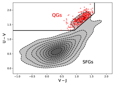
Figure 1: Rest-frame UVJ-color diagram. Red dots are the selected QGs in this study (section 2.1). Background grey contours show the density distribution of $1.2<z<4$ galaxies in the CANDELS/COSMOS. Black solid lines show the SFG-QG separation boundaries used in this work, where QGs are selected to be in the region enclosed by $U-V>0.88(V-J)+0.49$, $U-V>1.3$ and $V-J<1.6$.

The parent QG sample is selected to be in the redshift range between $1.2<$ $z_{\rm{obs}}$ $<4$ using either photometric, or spectroscopic redshift when available, and to have integrated isophotal signal-to-noise ratio SNR $>10$ in the HST/WFC3 $H_{160}$ band to ensure good photometric and imaging qualities. We also impose a low-end stellar mass cut, $\log_{10}(M_{*}/M_{\sun})=9$, to ensure good $M_{*}$ completeness in all fields ($\gtrsim 80\%$, see Ji et al. 2018 for CANDELS/GOODS and Nayyeri et al. 2017 for CANDELS/COSMOS). In addition, galaxies with clear evidence of AGN activity, i.e. those flagged using the AGNFlag in the photometric catalogs (section 2.2), have been removed from the sample. These criteria yield a total sample of 677 QGs, 288, 206 and 183 from CANDELS/COSMOS, GOODS-South and GOODS-North, respectively.

High-quality morphological measurements are crucial for this study. As we will detail in section 2.5, we use the GALFITFlag from van der Wel et al. (2012) to select QGs that have reliable single Sérsic Galfit fitting results. Equally crucial to this study is to have high-quality photometric data that densely samples the rest-frame UV-Optical-NIR SED of the galaxies, since this is essential to make the high-fidelity SFH reconstructions. Because the adopted catalogs contain photometry from different telescope/instrument combinations, whose depths and angular resolutions are different from one to another, the reliability of the photometry depends critically on the quality of the adopted de-blending procedures of low-resolution images. Given the relatively small sample size, we have visually inspected the galaxies of our sample in all bands to select QGs with high-quality photometry. Examples of galaxies following our visual inspections are illustrated in Figure 2. After removing the galaxies with either unreliable fitting results of Galfit or poor quality of photometry, the final sample consists 361 QGs, specifically 187, 123 and 51 from the CANDELS/COSMOS, GOODS-South and GOODS-North fields, respectively.

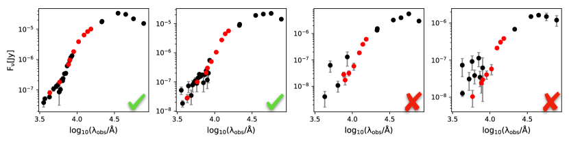
Figure 2: Examples of the photometry of individual UVJ-selected QGs that illustrate our procedure to visually inspect and clean our sample. Only photometry with SNR $>1$ is plotted here. Photometry from HST is marked in red. The left-most panel shows an example of the best case, where the photometry has high SNR and densely samples the galaxy’s SED. The second panel illustrates the next-to-best case, where increased photometric scatter is observed. The third panel shows an example where the galaxy’s SED is not as densely sampled as the first two cases. The right-most panel shows an example where the sampling of the SED is good but the photometric quality is much poorer than the previous cases, primarily due to the shallower depth and lower angular resolution of ground-based observations. To secure high-quality SFH reconstructions, we have limited our final sample only to the QGs with photometry like the first two examples.

2.2 Photometric data

Densely sampled ($\approx$ 40 bands) photometry, obtained from ground-based and space-borne instruments and covering the rest-frame UV-to-NIR spectral range for galaxies at $z\sim 2$, is available in all three fields.

In this work, we use the photometric catalog from Nayyeri et al. (2017) for the CANDELS/COSMOS field. For the GOODS-North field, we use the photometric catalog from Barro et al. (2019). In addition to the HST data taken during the GOODS (Giavalisco et al., 2004) and CANDELS surveys and other ground- and space-based ancillary data from UV to FIR, the 25 medium-band photometry at the optical wavelengths acquired during the SHARDS survey (Pérez-González et al., 2013), taken by the OSIRIS instrument at the Spanish 10.4-m telescope Gran Telescopio Canarias, is newly added to the catalog. Given the special characteristic of the OSIRIS, i.e. the varying passband seen by different parts of the detector, each galaxy has its unique set of passbands. As a result, for each galaxy, this requires us to shift the nominal bandpass of every filter to the actual central wavelength measured by Barro et al. (2019) prior to SED fitting (section 2.3).

Finally, for the GOODS-South field, we use the latest photometric catalog from the ASTRODEEP project (ASTRODEEP-GS43, Merlin et al. 2021). Compared with the old Guo et al. 2013 catalog in the GOODS-South, this new one uses the latest and improved version of the template-fitting software T-PHOT (Merlin et al., 2016) to de-blend low angular-resolution images based on positional priors from high angular-resolution ones to derive aperture matched fluxes. In addition, this new catalog adds 18 new medium-band photometric data observed with the Subaru SuprimeCAM (Cardamone et al., 2010), and another 5 photometric bands observed with the Magellan Baade FourStar (Straatman et al., 2016).

2.3 SED fitting with Prospector

We use the panchromatic photometry described above to perform SED modeling for the sample QGs using Prospector (Leja et al., 2017; Johnson et al., 2021), with specific emphasis on the robust reconstruction of their SFHs and also to obtain an independent measure of $M_{*}$.

Prospector is an SED fitting code built upon a fully Bayesian inference framework, and importantly, it allows flexible parameterizations of SFHs, which has been extensively shown to be critical for characterizing the diversity of the assembly history of galaxies and for unbiasedly measuring the physical properties such as the age of stellar populations (e.g. Lee et al., 2018; Carnall et al., 2018; Iyer et al., 2019; Leja et al., 2019a; Tacchella et al., 2022). Regarding the basic setup of Prospector, we adopt the Flexible Stellar Population Synthesis (FSPS) code (Conroy et al., 2009; Conroy & Gunn, 2010) where the stellar isochrone libraries MIST (Choi et al., 2016; Dotter, 2016) and the stellar spectral libraries MILES (Falcón-Barroso et al., 2011) are used. During the modeling, we use the sampling code dynesty (Speagle, 2020) which adopts the nested sampling procedure (Skilling, 2004) that simultaneously estimates the Bayesian evidence and the posterior.

In this work, we assume the Kroupa 2001’s initial mass function (IMF) for consistency with the IMF used in the Byler et al. 2017’s nebular continuum and line emission model, which we adopt in our SED modeling. We assume the Calzetti et al. 2000’s dust attenuation law and fit the V-band dust optical depth with an uniform prior $\tau_{V}\in(0,2)$. We also set redshift as a free parameter, but with a strong prior: a normal distribution centers at the best redshift value from the CANDELS catalogs (either photometric or secure spectroscopic redshift whenever available), with a width equal to the corresponding redshift uncertainty.

Similar to what has been extensively assumed in literature, we leave the stellar metallicity ($Z_{*}$) of galaxies as a free parameter during the SED modeling, meaning that we assume all stars in a galaxy have the same $Z_{*}$. In this way the detailed history of metal enrichment is ignored. We use a uniform prior in the logarithmic space $\log_{10}(Z_{*}/Z_{\sun})\in(-2,0.19)$, where $Z_{\sun}=0.0142$ is the solar metallicity, and the upper limit of the prior is chosen because it is the highest value of metallicity that the MILES library has. Measuring accurate $Z_{*}$ is beyond the scope of this work, as it requires deep spectroscopic data. Nevertheless, we have checked the measurements by fixing $Z_{*}=Z_{\sun}$ during the SED fitting (see Appendix C), finding no substantial changes in the parameters of our interests.

Our fiducial model assumes a non-parametric piece-wise SFH composed of $\rm{N_{SFH}=9}$ lookback (i.e. the time prior to the time of observations) time bins, where the value of the star formation rate (SFR) is constant within each bin. Among the intervals of the nine bins, the first two bins are fixed to be $0-30$ and $30-100$ Myr to capture, with relatively higher time resolution, recent episodes of star formation; the last bin is assumed to be $\rm{0.9t_{H}-t_{H}}$ where $\rm{t_{H}}$ is the age of the Universe at $z_{\rm{obs}}$; the remaining six bins are evenly spaced in the logarithmic lookback time between 100 Myr and $\rm{0.9t_{H}}$. As already extensively explored by Leja et al. (2019a) using mock observations generated from cosmological simulations (see their section 2.1 and Figure 15), the recovered physical properties, including the age of stellar populations, generally are insensitive to $\rm{N_{SFH}}$ once it is greater than five.

As highlighted by Leja et al. (2019a), because the procedure above to model non-parametric SFHs includes “more bins than the data warrant”, it potentially suffers from overfitting problems which are caused by the excessive model flexibility and can lead to overestimated uncertainties. This issue can be effectively mitigated by choosing a prior to weight for physically plausible forms of SFHs (e.g. Carnall et al. 2019a; Leja et al. 2019a). Following this suggestion, we use the well-tested Dirichlet prior (Leja et al., 2017) as our fiducial model. We refer readers to those references for the mathematical details of the Dirichlet prior. Here we only outline several key features. The Dirichlet distribution describes a distribution for N parameters $f_{i}\in(0,1)$ whose summation satisfies the constraint $\sum_{i=1}^{N}f_{i}=1$. Instead of directly modeling the $M_{*,i}$ formed in each lookback time bin, the Dirichlet prior parameterizes a non-parametric SFH as the normalization of the SFH using the total $M_{*}$ formed by the time of $z_{\rm{obs}}$, and the shape of the SFH using the $(\rm{N_{SFH}}-1)$ fractional mass $m_{i}$ formed in each time bin,

$$m_{i}=\frac{\delta t_{i}f_{i}}{\sum_{i=1}^{\rm{N_{SFH}}}\delta t_{i}f_{i}}$$ (1)

where $f_{i}$ is the Dirichlet parameter and $\delta t_{i}$ is the width of each time bin. In our case, an uniform prior is assumed for logarithmic stellar mass $\log_{10}(M_{*}/M_{\sun})\in(9,12)$. An additional concentration parameter $\alpha_{D}$ is required for the Dirichlet distribution. The case of $\alpha_{D}\geq 1$ means distributing weight more evenly to all time bins (a smoother SFH) while the opposite case means distributing all weights to a single time bin (a burstier SFH). We decide to fix $\alpha_{D}=1$ as it has been demonstrated to work very well across various forms of SFHs (Leja et al., 2019a). Finally, the Dirichlet prior returns a symmetric prior on stellar age and specific SFR (sSFR=SFR$/M_{*}$), and a constant SFH prior with $\rm{SFR(t)=M_{*}/t_{H}}$. Meanwhile, because the Dirichlet prior does not enforce a smooth transition in SFR across adjacent time bins, this means it allows events such as fast quenching and rejuvenation to happen inside galaxies.

We have also experimented using the other non-parametric SFH prior, namely the Continuity prior, which enforces smooth changes of SFR in adjacent time bins (see Leja et al. 2019a for details) and has been used in some recent studies (e.g. Leja et al., 2019b; Tacchella et al., 2022). We first use synthetic galaxies from the IllustrisTNG cosmological simulation (Nelson et al., 2018; Springel et al., 2018; Marinacci et al., 2018; Pillepich et al., 2018; Naiman et al., 2018) to validate our fiducial Prospector fitting procedure, and then we compare the recovered physical properties derived from the two different priors of non-parameteric SFHs with the intrinsic properties obtained from the simulations (see Appendix A). From this comparison we find that the Dirichlet prior works better than the Continuity prior given the typical wavelength coverage and photometric quality of our sample. While tests with simulations provide very valuable guidance to assess the performance of the SED fitting procedure, they are also very limited because it is hard to assess the accuracy of how the simulations model the SFH of real galaxies. We thus decide to additionally do an empirical test where we run a new set of Prospector SED fittings for our QGs using the Continuity prior, with the specific goal to quantify the dependence of the physical parameters of our interests on the adopted prior (see Appendix B). While systematic offsets are observed, strong and tight correlations are observed among the same parameters derived using the two different priors, meaning that switching to the Continuity prior will not qualitatively change any conclusion of this work. We have ultimately decided to adopt the measurements from the Dirichlet prior as the fiducial ones, because this prior works better according to the IllustrisTNG-based tests that we have conducted.

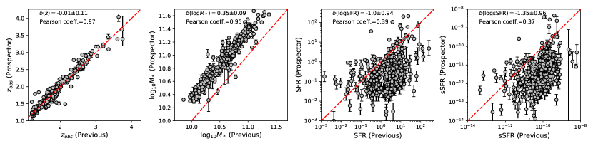
Figure 3: Comparisons between parameters derived from our Prospector fitting (y-axis) and from previous (x-axis) measurements (see section 2.3 for details). Also labelled in each panel are the median and standard deviation of the difference between the two measurements, and the Pearson correlation test coefficient between the two measurements. The red dashed line marks the one-to-one relation.

We now move to check the consistency of our new Prospector SED fitting results with existing previous measures. We use the previous measurements from Lee et al. (2018) for the CANDELS/GOODS fields, and from Nayyeri et al. (2017) for the CANDELS/COSMOS field. In Figure 3 we compare the Prospector-derived $z_{\rm{obs}}$, $M_{*}$, SFR and sSFR to the previous measures. We also run Pearson correlation tests between the two measurements. In all cases we find strong correlations, showing the consistency between the Prospector and the previous measurements.

Specifically, excellent agreement is seen for $z_{\rm{obs}}$. A strong and rather tight correlation is also seen for $M_{*}$, although a +0.35 dex offset, $\delta(\log M_{*})=\log M_{*}(\rm{Prospector})-\log M_{*}(\rm{Previous})$, is found. We note that the previous measurements above have been obtained assuming the Chabrier (2003)’s IMF which is different from the Kroupa (2001)’s IMF adopted by our Prospector fitting. This however is insufficient to account for the observed offset, as the difference in $M_{*}$ caused by the two IMFs is typically $\approx 10\%$ only (e.g. Speagle et al., 2014). The real cause of the systematic shift in the $M_{*}$ measurements comes from the different SFHs assumed during SED modeling. Unlike the non-parametric form of SFHs assumed in our Prospector modeling, the adopted Nayyeri et al. measurements assumed an exponential declining SFH (SFR$(t)\propto e^{-t/\tau}$). Although the Lee et al. measurements left the form of SFH as a free parameter during their SED fitting, this could only vary among five parametric functional forms, and they found that the majority of QGs prefer an exponential declining SFH as the best-fit solution (see their Figure 2). Using non-parametric SFHs returns older stellar ages, and hence larger stellar masses, than using parametric ones (see Carnall et al. 2019a; Leja et al. 2019a, 2021 for details). Evidence that the larger stellar masses are actually more accurate has been found. Using synthetic galaxies generated from cosmological simulations, Lower et al. (2020) showed that the $M_{*}$ derived from non-parametric SFHs is closer to the intrinsic value and it can be as much as $0.3-0.5$ dex larger than that derived from parametric SFHs, which is quantitatively similar to the offset of $M_{*}$ measurements seen here. Leja et al. (2020) showed that the SFHs inferred from the non-parametric method are more consistent with the observed evolution of galaxy stellar-mass function over $0.5<z<3$. In addition, Leja et al. (2021) showed that using the SFR and $M_{*}$ derived from non-parametric SFHs can solve a long-standing systematic offset of the star-forming main sequence between observations and predictions from cosmological simulations (see their section 7.1).

Accurately measuring SFR is very challenging for QGs (Conroy, 2013) and the results critically depend on the assumed form of SFHs. The adoption of non-parametric forms by Prospector appears to provide substantial improvements if adequate wavelength coverage of galaxy’s SED is available (Leja et al., 2019b). Comparing our new results with previous ones shows that although a correlation with a Pearson correlation coefficient $\approx 0.4$ is seen between the two sets of SFR measurements, the scatter, unsurprisingly, is much larger than that of $z_{\rm{obs}}$ and $M_{*}$. A similar behavior is also observed when comparing the measurements of sSFR. In the Figure we compare the Prospector-derived instantaneous SFR, which in our case is essentially the SFR averaged over the past 30 Myr (the first time bin of the assumed SFHs), to the previous SFR measures. These include a mix of measures from the SED fitting and also from $\rm{SFR_{UV}^{obs}+SFR_{IR}}$ diagnostics (see Lee et al. 2018 for details). We find that in addition to the increased scatter of the correlation, the former is smaller than the latter by $\approx 1$ dex. In part, this reflects the different methodology adopted for the SED fitting, as discussed before. In part, this also reflects the fact that, especially for QGs, the $\rm{SFR_{UV}^{obs}+SFR_{IR}}$ diagnostics are affected by significant contributions to the IR flux from AGB stars and/or dust heated by old stars or AGN (e.g. Salim et al., 2009; Fumagalli et al., 2014; Hayward et al., 2014), rather than on-going star formation, making the latter SFR only an upper limit. Regardless of the offset and scatter seen in the SFR and sSFR comparisons, our SED fitting with Prospector consistently shows that the QGs pre-selected through the UVJ technique have low sSFR $\lesssim 10^{-10}\rm{yr}^{-1}$, confirming the quiescent nature of the sample galaxies.

2.4 Characterizing the shape of SFHs

In this section we introduce the parameters, which are derived from the reconstructed non-parametric SFHs and take into account the information contained in their shapes, to quantitatively describe the epochs and timescales of SFHs. Similar to what has been done in recent literature, the first set of parameters are characteristic redshifts, including

• $z_{\rm{form}}$ (formation redshift): the redshift when the time interval between $z_{\rm{form}}$ and $z_{\rm{obs}}$ equals to the mass-weighted age ($t_{\rm{age}}$) of a galaxy

• $z_{\rm{p}}$ (p$=50,70,90$): the redshift when p-percent $M_{*}$ seen by the time of $z_{\rm{obs}}$ have already formed.

We point out that the definition of $z_{\rm{form}}$ is very similar to that of $z_{50}$, and the difference between the two is only 5% on average and 21% at most. In addition, the uncertainty of $z_{\rm{p}}$ increases as p becomes smaller because of the large uncertainty in estimating the contributions from older stellar populations given the data coverage we currently have (Papovich et al., 2001). Tacchella et al. (2022) used the time intervals between two $z_{\rm{p}}$ as proxies for the timescales of star formation and quenching of galaxies. While this is able to describe the general shape of SFHs, the choice of the values of p is somewhat arbitrary, and it is unable to describe other possible features of SFHs such as star-formation rejuvenation. Instead of using arbitrary time epochs (e.g. $z_{\rm{p}}$), we propose a new set of parameters that utilize the information of the full shape of SFHs. In this way the aforementioned drawbacks can be mitigated. The new parameters are detailed as follows.

The first parameter $\tau_{\rm{tot}}$ measures the width (i.e. duration) of the main star-formation episode of an SFH,

$$\tau_{\rm{tot}}=2\times\sqrt{\frac{\int_{0}^{t_{\rm{H}}}(t-t_{\rm{age}})^{2}\cdot\rm{SFR}(t)dt}{\int_{0}^{t_{\rm{H}}}\rm{SFR(t)}dt}}.$$ (2)

This definition is essentially the square root of the mass-weighted second central moment of stellar ages, times the factor two to account for the full (two-side) width. In our case, since the SFH has a constant piece-wise shape with nine time bins, the equation above can be re-written as

$$\tau_{\rm{tot}}=2\times\sqrt{\frac{\sum_{i=1}^{9}\,(t_{i}-t_{\rm{age}})^{2}\cdot\rm{SFR}_{i}\delta t_{i}}{M_{*}}}.$$ (3)

In the middle panel of Figure 4, we plot the reconstructed SFHs for the subsample of QGs within a narrow redshift ($z_{\rm{obs}}=1.7-2.2$) and stellar mass ($\log_{10}M_{*}=10.7-11.2$) ranges. We divide the subsample into two groups using its median $\tau_{\rm{tot}}$. It can be seen in Figure 4 that the group having larger $\tau_{\rm{tot}}$ also has a more extended period of star-formation episode.

Another important characteristic is the overall asymmetry of SFHs which contains key information of the relative timescale between the period of actively forming stars and the period of the quenching of star formation. We introduce two ways to quantify this property. The first one is the Skewness, i.e. the third standardized moment of stellar ages,

$$\begin{split}\rm{Skewness}=\frac{1}{(0.5\tau_{\rm{tot}})^{3}}\cdot\frac{\int_{0}^{t_{\rm{H}}}(t-t_{\rm{age}})^{3}\cdot\rm{SFR}(t)dt}{\int_{0}^{t_{\rm{obs}}}\rm{SFR(t)}dt}\\ =\frac{8}{\tau_{\rm{tot}}^{3}}\cdot\frac{\sum_{i=1}^{9}\,(t_{i}-t_{\rm{age}})^{3}\cdot\rm{SFR}_{i}\delta t_{i}}{M_{*}}\end{split}$$ (4)

A more positive Skewness means that an SFH has a longer tail towards $t>t_{\rm{age}}$, which is demonstrated in the right-most panel of Figure 4. The other way is to first divide an SFH into two parts, namely an actively star-forming period when $t_{\rm{age}}<t<t_{\rm{H}}$ and a quenching period when $0<t<t_{\rm{age}}$, and then directly compare the time widths between the two periods, i.e. $\tau_{\rm{SF}}/\tau_{\rm{Q}}$, where

$$\begin{split}\tau_{\rm{SF}}=\sqrt{\frac{\int_{t_{\rm{age}}}^{t_{\rm{H}}}(t-t_{\rm{age}})^{2}\cdot\rm{SFR}(t)dt}{\int_{t_{\rm{age}}}^{t_{\rm{H}}}\rm{SFR(t)}dt}}\\ \tau_{\rm{Q}}=\sqrt{\frac{\int_{0}^{t_{\rm{age}}}(t-t_{\rm{age}})^{2}\cdot\rm{SFR}(t)dt}{\int_{0}^{t_{\rm{age}}}\rm{SFR(t)}dt}}\end{split}.$$ (5)

For our measurements, we replace both integrals with discrete summations in the same way as we did for $\tau_{\rm{tot}}$ and the Skewness. We have compared the Skewness and $\tau_{\rm{SF}}/\tau_{\rm{Q}}$ in Appendix D, where we find that these two metrics are highly consistent with each other in quantifying the asymmetry of SFHs. We also show that combining the two metrics can effectively identify the subtle events such as star formation rejuvenation in SFHs.

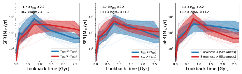
Figure 4: Demonstration of the effectiveness of the metrics introduced in section 2.4 to quantitatively characterize the shape of reconstructed SFHs. In the plots we only show the SFHs, expressed as SFR versus lookback time from $z_{\rm{obs}}$, for the QGs within narrow ranges of redshift and stellar mass, namely $1.7<z_{\rm{obs}}<2.2$ and $10.7<\log_{10}(M_{*}/M_{\sun})<11.2$. A full collection of reconstructed SFHs is shown in Figure 6. From left to right the QGs are divided into two groups using the sample median value of $\langle t_{\rm{age}}\rangle$, $\langle\tau_{\rm{tot}}\rangle$ and $\langle$Skewness$\rangle$ (check section 2.4 for parameter definitions). The thin dashed line shows the individual SFHs. The SFH averaged over each group is shown as a thick solid line (median) with a shaded region (16-84th percentile range).

2.5 Morphological properties

Morphological measurements of individual QGs are taken from van der Wel et al. (2012), where the morphology of galaxies is described in terms of their light profiles modeled with a single Sérsic function using Galfit (Peng et al., 2010a). To secure robust measurements, we only use those with the best quality flag, namely GALFITFlag = 0, following the recommendation of van der Wel et al.. This means that we exclude the galaxies whose single Sérsic fitting (1) has a suspicious result where the Galfit magnitude significantly deviates from the expected magnitude derived from SExtractor (Bertin & Arnouts, 1996), or (2) has a bad result where at least one parameter reaches the constraint value (e.g. $0.2<n<8$, $b/a>0.1$) set to Galfit, or (3) is unable to converge.

We use the measurements in the $H_{160}$ band because it better probes the stellar morphology for $z\sim 2$ galaxies as it is the reddest HST imaging data available in the three fields. Throughout this work, all morphological parameters are measured in the $H_{160}$ band unless specified otherwise. For each QG, we obtain the half-light radius $R_{\rm{e}}$ (circularized, $=R_{e,maj}\sqrt{b/a}$) and the Sérsic index $n$. Together with $M_{*}$ derived from the SED fitting, we obtain the projected stellar mass surface density inside the effective radius $\Sigma_{e}$ ($=M_{*}/(2\pi R_{e}^{2})$) and inside the central radius of 1 kpc (Cheung et al., 2012),

$$\Sigma_{\rm{1kpc}}=\frac{M_{\rm{1kpc}}}{\pi\cdot 1\rm{kpc}^{2}}=\frac{M_{*}}{\pi\cdot 1\rm{kpc}^{2}}\frac{\gamma(2n,\,x)}{\Gamma(2n)}$$ (6)

where $x=b_{n}(\frac{1\rm{kpc}}{R_{e}})^{1/n}$, $\gamma/\Gamma$ is the ratio of incomplete gamma function divided by complete gamma function, and $b_{n}$ is calculated by numerically solving $\Gamma(2n)=2\gamma(2n,b_{n})$ (Graham & Driver, 2005).

The measurements of $R_{\rm{e}}$ and $n$ are usually highly covariant, making the determination of best-fit values of the individual parameters ($n$ in particular) highly uncertain (e.g. Ji et al., 2020). As discussed in Ji et al. (2022), because $\Sigma_{\rm{1kpc}}$ is derived as the combination of $R_{\rm{e}}$ and $n$, this helps to reduce the uncertainty stemming from the strong covariance between the two parameters, making $\Sigma_{\rm{1kpc}}$ significantly better constrained than the two parameters individually. In this sense, $\Sigma_{\rm{1kpc}}$ is a more robust outcome of the light profile modeling procedure than $n$.

In addition, because $\Sigma_{e}$ and $\Sigma_{\rm{1kpc}}$ strongly correlate with $M_{*}$, any correlation observed with $\Sigma$ then can in principle be driven by $M_{*}$ rather than galaxy morphology. This motivates the use of the fractional mass within the central radius of 1kpc,

$$\frac{M_{1\rm{kpc}}}{M_{*}}=\frac{\pi(\rm{1kpc})^{2}\Sigma_{\rm{1kpc}}}{M_{*}}=\frac{\gamma(2n,\,x)}{\Gamma(2n)},$$ (7)

which was introduced by Ji et al. (2022), and has been demonstrated to be able to quantify the compactness of galaxies while removing most of the dependence on $M_{*}$.

3 Results

We use the reconstructed SFHs of the QGs to study the relationships of their assembly history with $M_{*}$, size and other morphological properties. In section 3.1, we show the diverse assembly history of QGs. In section 3.2, we study the dependence of the assembly history of QGs on $M_{*}$. In section 3.3, we explore the relationship between the assembly history of QGs and $R_{\rm{e}}$. In section 3.4, we carry out the stacking analysis to further study the relationship between the multi-band light distribution of QGs and their assembly history. Finally, in section 3.5, we explore the relationships between the compactness of QGs and their assembly history.

3.1 The Diverse Assembly History of QGs

To begin, we show the diverse assembly history of QGs by plotting $t_{\rm{age}}$ as a function of $z_{\rm{obs}}$. Figure 5 shows that at fixed $z_{\rm{obs}}$ QGs are a mixture of those that have been quenched for a long time and those that have just quenched. The span of $t_{\rm{age}}$ is $\approx 0.3\sim 2.5$ Gyr at fixed $z_{\rm{obs}}$, being very similar to the range of stellar ages measured by Belli et al. (2019) for a sample of 24 QGs at $z\sim 1.6$ using the rest-frame optical spectra taken by the Keck/MOSFIRE, and by Carnall et al. (2019b) for a sample of 75 QGs at $z\sim 1.1$ using the rest-frame UV/Optical spectra taken by the VLT/VIMOS, as well as by Estrada-Carpenter et al. (2020) for a sample of QGs at $0.7<z<2.5$ using low-resolution spectra taken by the HST/G102 and G141 grisms. If we plot the expected stellar age of single stellar populations (SSPs) formed at different redshifts, we find that most of our QGs fall between the SSPs formed between $z=1.5$ and $z=8$. This is consistent with the measurements of Tacchella et al. (2022) for a sample of lower-redshift ($z\sim 0.8$) QGs using the deep rest-frame optical spectra taken by the Keck/DEIMOS. We note that the $t_{\rm{age}}$ of some QGs in our sample suggests that they have formed at $z\sim 8$ when the Universe was only $\approx 0.6$ Gyr old. This means that they have assembled most of their mass within a very short period of time since the Big Bang. These QGs provide an excellent test bed of the history of metal enrichment in galaxies in the early Universe and the formation of the First Galaxies. This idea has been exploited by Kriek et al. (2016), who carried out ultradeep rest-frame optical spectroscopy with the Keck/MOSFIRE for a $z=2.1$ QG and reported a [Mg/Fe] $\approx$ 0.6 which is consistent with that the galaxy has formed at $z\approx 10$.

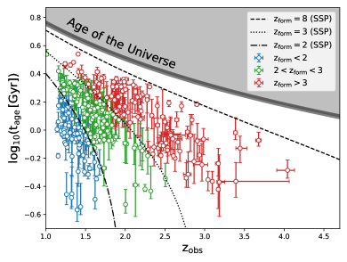
Figure 5: The relationship between mass-weighted age ($t_{\rm{age}}$, vertical axis) and observed redshift ($z_{\rm{obs}}$, horizontal axis). Individual QGs are color-coded according to their $z_{\rm{form}}$. The thick grey line marks the age of the Universe. The dotted, dashed and dot-dashed lines present the expected age for a single stellar population (SSP) formed at $z=8$, $z=3$ and $z=2$ respectively.

In Figure 6 we present the full collection of the reconstructed SFHs of our sample galaxies. Also marked in Figure 6 is the relation of $1/(10t_{\rm{H}}(z))$. Because the inverse of sSFR is the mass-doubling time of galaxies assuming that they continue forming stars with the current SFR, when the sSFR is below the marked relation, this means the mass-doubling time is longer than even 10$\times$ the age of the Universe, implying a very low level of star formation. At fixed $z_{\rm{obs}}$, QGs with larger $M_{*}$ have lower sSFR at the time of observations. Meanwhile, at fixed $M_{*}$, QGs observed at higher $z_{\rm{obs}}$ have higher sSFR. This is consistent with the downsizing effect of galaxy formation (Cowie et al., 1996). A closer inspection of the variety of shapes of the individual SFHs reveals a broad diversity of assembly history. Looking at QGs with similar $M_{*}$ and $z_{\rm{obs}}$ shows that some have quickly become quiescent after an initial, relatively rapid burst of star formation, while others have experienced a more extended assembly history, with some showing multiple episodes of enhanced star formation activity before $z_{\rm{obs}}$.

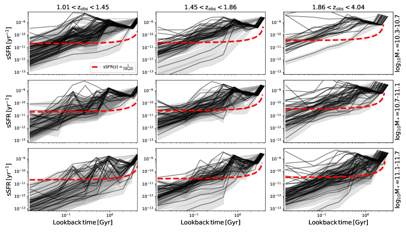
Figure 6: The collection of the reconstructed SFHs. The sample is divided in intervals of $z_{\rm{obs}}$ and $M_{*}$, where $z_{\rm{obs}}$ increases from left to right and $M_{*}$ increases from top to bottom. The y-axis is plotted as sSFR. The red dashed line marks the relation of $1/(10t_{\rm{H}}(z))$. sSFR below the red dashed line indicates a very low level of star formation.

In Figure 7 we plot the distributions of the individual characteristic parameters of SFHs introduced in section 2.4. All parameters span quite wide ranges, again illustrating the diversity of the assembly history of QGs. Using $\tau_{\rm{tot}}$ as a proxy, the median timescale of the main star-forming episode inside our $z\sim 2$ QG sample is 1.17 Gyr with a 0.58 Gyr standard deviation of the distribution. This is in quantitative agreement with spectroscopic studies of QGs at $z>1$. For example, Kriek et al. (2019) used elemental abundances [Fe/H] and [Mg/Fe], measured using the spectra taken by the Keck/LRIS and MOSFIRE for a sample of five massive QGs, to constrain the star-formation timescale to be 0.2$-$1 Gyr at $z\sim 1.4$. The agreement is tantalizing, especially since the data sets and methodologies used are dramatically different. The histograms of $\tau_{\rm{SF}}$ and $\tau_{\rm{Q}}$ also reflect the relatively longer duration of the star-forming phase, i.e. the time span before the peak of the SFH, relative to the quenching phase, namely the period past the peak. The former is about 1 Gyr long on average, while the latter is half as long, reinforcing the conclusions of a large body of research that consistently suggests that quenching is generally a comparatively shorter process than star formation (e.g. Barro et al., 2013; Renzini & Peng, 2015; Estrada-Carpenter et al., 2020; Chen et al., 2020; Tacchella et al., 2022). The diversity of the assembly history of QGs is also reflected in the very broad distributions of the Skewness and of $\tau_{\rm{SF}}$/$\tau_{\rm{Q}}$. Both parameters describe the relative timescales of the star formation and quenching of high-redshift QGs. While the focus of this paper is on the progenitor effect, rather than on quenching, in an another, upcoming paper of this series we will address the relationship between the structure of galaxies and the Skewness and $\tau_{\rm{SF}}$/$\tau_{\rm{Q}}$ of their SFHs.

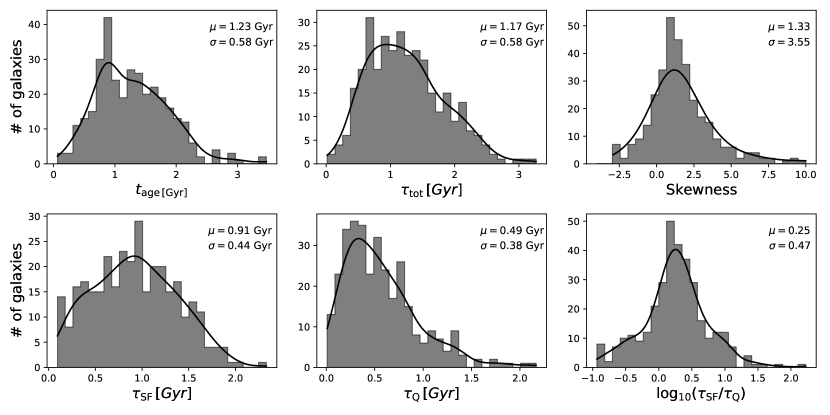
Figure 7: Histograms of the key parameters used to quantify the shape of SFHs. We refer readers to section 2.4 for the definition of individual parameters in detail. Overplotted black solid curve show the underlying density distributions estimated using a Gaussian kernel. The median and standard deviation are also labelled for each distribution.

Finally, we combine $z_{\rm{form}}$, $\tau_{\rm{tot}}$ and $\tau_{\rm{SF}}$/$\tau_{\rm{Q}}$, and plot them together as a single scatter plot which is shown in Figure 8. Again, the diverse assembly history of QGs can be clearly recognized. The $\tau_{\rm{tot}}$ spans the entire range from $\sim 0.1$ Gyr to the age of the Universe at $z_{\rm{form}}$, meaning that for the QGs formed at the similar epoch of the Universe, the timescale of their mass assemblies can be dramatically different. While the reconstructed SFHs suggest that some of the QGs have experienced a rapid monolithic assembly history (small $\tau_{\rm{tot}}$), namely that they have assembled most of their mass within a very short period of time, other QGs have assembled their mass following a much more smoother and extended process (large $\tau_{\rm{tot}}$).

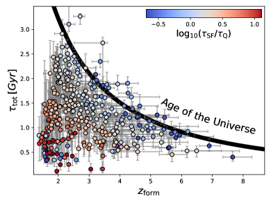
Figure 8: The relationship between $z_{\rm{form}}$ and $\tau_{\rm{tot}}$. Each point is color-coded using $\tau_{\rm{SF}}$/$\tau_{\rm{Q}}$. The age of the Universe at $z_{\rm{form}}$ is also shown as the black solid line.

3.2 The Stellar Mass of QGs and Their Assembly History

In this section we study the relationship between $M_{*}$ and the assembly history of QGs. In Figure 9, $M_{*}$ is plotted against $z_{\rm{form}}$. While the entire discussions of this work focus only on $\geq 10^{10.3}M_{\sun}$ QGs where the environmental effects should only play a relatively minor role, we also include $<10^{10.3}M_{\sun}$ QGs to the plot here, just to illustrate the entire UVJ-selected QG sample in the CANDELS/COSMOS and GOODS fields.

To begin, $z_{\rm{form}}$ spans a wide range from 1.5 to 6 at fixed $M_{*}$, which is very similar to the ranges found by other studies of high-redshift QGs (Saracco et al., 2019; Carnall et al., 2019b; Estrada-Carpenter et al., 2020; Tacchella et al., 2022). The range of $z_{\rm{form}}$ also becomes wider as QGs are more massive. For a more quantitative comparison, we fit a linear relation between $M_{*}$ and $t_{\rm{age}}$. The best-fit relation (the orange solid line in Figure 9) is found to be

$$\frac{t_{\rm{age}}}{Gyr}=2.46^{+0.07}_{-0.04}-1.23^{+0.14}_{-0.21}\cdot\log_{10}(\frac{M_{*}}{10^{11}M_{\sun}})$$ (8)

where the uncertainties of best-fit parameters are estimated as follows. We first bootstrap the sample, during which we also resample the value of each measurement using a normal distribution with the uncertainties of $t_{\rm{age}}$ and $M_{*}$ derived from Prospector fitting results. We then repeat the process 1000 times, and get the 1$\sigma$ uncertainty for the best-fit relation. In this way both sample random errors and measurement uncertainties are taken into account.

Carnall et al. (2019b) and Tacchella et al. (2022) also performed the same linear fit using their measurements, which are shown as the red and blue dashed lines in Figure 9. Compared with our QGs, their samples are at lower redshift $0.5<z<1.3$ where rest-frame UV/optical spectroscopy is still feasible for statistically significant QG samples using current instrumentations. Both studies included spectra to their SED modellings for the SFH reconstructions. We find very good agreement between our best-fit relation and that of Carnall et al. (2019b), suggesting that the SFH of QGs can be robustly reconstructed even without spectroscopy, if sensitive, panchromatic photometry is available (also see Appendix A for our tests with simulated galaxies). In fact, given that in both Carnall et al. and Tacchella et al. cases the wavelength range of spectral coverage is very narrow, and because the accurate absolute flux calibration for the ground-based spectroscopic data is challenging, the continuum shape is modelled using the polynomials rather than a pure stellar synthesis model. Unless the spectra have multiple detections of stellar spectral features (e.g. absorptions) with high SNRs, the real information gained from the spectra is limited.

A $\approx 0.4$ Gyr offset is seen between our best-fit relation and that of Tacchella et al. (2022). This is unlikely due to the sample selection effects, because all QGs are selected using the UVJ technique and the $M_{*}$ distributions are very similar. While Tacchella et al. (2022) also used Prospector, they assumed the Continuity prior while we are using the Dirichlet prior. As one can see in detail in Appendix A, compared with the Dirichlet prior, using the Continuity prior over-estimates $t_{\rm{age}}$ by $\approx 0.5$ Gyr for the Illustris-TNG QGs at $z\sim 2$, which is quantitatively consistent with the offset seen here. We therefore believe the offset is primarily caused by different assumptions on the prior of non-parametric SFHs. Although the magnitude of the offset is small (within 0.5$\sigma$) compared to the dispersion of the relation (next paragraph), nevertheless, it immediately shows the potentially significant systematics introduced by priors for the similar studies, and also highlights the importance in understanding the imprint of the priors on the reconstructed SFHs.

We also measure the percentile trends between $z_{\rm{form}}$ and $M_{*}$. We adopt the non-parametric quantile regression method, in which case no arbitrarily defined bins are required. We use the COnstrained B-Splines (cobs, see Ng & Maechler 2007, 2020 for details) package in R where the total number of knots required for the regressions B-spline method is determined using the Akaike-type information criterion. The resulting median (black solid line), 31th-69th percentiles ($\approx 0.5\sigma$, dark grey shaded region) and 16th-84th percentiles trends ($1\sigma$, light grey shaded region) are plotted in Figure 9. We see that the measurements of Tacchella et al. (2022) fall well within the 0.5$\sigma$ range of our measurements. Compared with the best-fit linear relation, a clear uptick is seen at the high-mass end ($>10^{11.5}M_{\sun}$). Although the significance of this uptick suffers from small number statistics, Tacchella et al. (2022) indeed also found very high $z_{\rm{form}}$ for their $>10^{11.5}M_{\sun}$ galaxies (see their Figure 11).

Finally, while in the discussions above only $z_{\rm{form}}$ is considered, in Appendix E we also show the relationships of $M_{*}$ with other characteristic redshifts, including $z_{50}$, $z_{70}$ and $z_{90}$. Very similar trends, namely that more massive QGs formed earlier, are observed, confirming the findings above when we use $z_{\rm{form}}$.

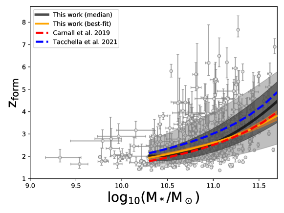
Figure 9: The relationship between $z_{\rm{form}}$ and $M_{*}$. While we only study the QGs with $\log_{10}(M_{*}/M_{\sun})\geq 10.3$ in this work, the plots here show all UVJ-selected QGs in the CANDELS/COSMOS, GOODS-South and GOODS-North. We use the COnstrained B-Splines package in R (Cobs) to carry out the non-parametric inter-quantile regressions. The median (black solid line), 31th-69 percentiles (0.5$\sigma$, dark grey shaded region) and 16th-84th percentiles (1$\sigma$, light grey shaded region) relations are plotted in the panel. The orange solid line and the shaded region show the best-fit and 1$\sigma$ range of the linear relation between $t_{\rm{age}}$ and $M_{*}$ (see Section 3.2 for details). Also shown as the red and blue dashed lines are the best-fit relations from Carnall et al. (2019b) and Tacchella et al. (2022), respectively.

3.3 The Size Evolution of QGs and Their Assembly History

In this section we study the relationship between the size evolution of QGs and their assembly history. In Figure 10, the effective radius $R_{\rm{e}}$ is plotted against $z_{\rm{form}}$. A linear fit is conducted in the logarithmic space, i.e.

$$\log_{10}R_{\rm{e}}=-\beta\log_{10}(1+z_{\rm{form}})+C.$$ (9)

The uncertainty of the best-fit relation is derived in the same way as we did in section 3.1 for the linear relation between $t_{\rm{age}}$ and $M_{*}$.

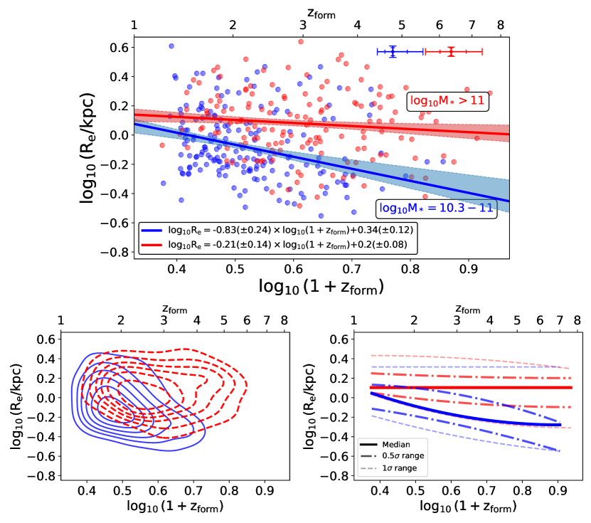
Figure 10: The relationship between $R_{\rm{e}}$ and $z_{\rm{form}}$. Top: The dots represent individual QGs with $10^{10.3}M_{\sun}<M_{*}<10^{11}M_{\sun}$ (lower-mass, shown in blue) and $M_{*}>10^{11}M_{\sun}$ (higher-mass, shown in red). The typical uncertainty of individual measurements is plotted in the upper-right corner, where the inner and outer error bars show the median and 84-th percentile of the individual uncertainties, respectively. The thick solid lines show the least squares linear regressions, and the light shaded regions show the 1$\sigma$ uncertainties. The best-fit relations and their uncertainties are labelled in the figure legend. Bottom left: The density distributions for the lower-mass and higher-mass QGs estimated using a Gaussian kernel. Bottom right: The median, 0.5$\sigma$ and 1$\sigma$ quantile trends derived using the Cobs.

The slope of the relation contains key information about the physics of galaxy size evolution. One should note that the Virial radius $R_{\rm{vir}}$ of a dark matter halo is set by the Virial density which by construction is the density contrast relative to the mean density of the Universe at the formation epoch of the halo and that it has a very weak time dependence, i.e. is essentially constant. This means that at fixed mass the size of halos formed at different redshifts should scale following the expansion of the Universe, i.e. $R_{\rm{vir}}\propto(1+z_{\rm{form}}^{\rm{h}})^{-1}$ (Mo et al., 2010). Note that to differentiate from $z_{\rm{form}}$ of a galaxy we use $z_{\rm{form}}^{\rm{h}}$ as the formation redshift of a halo. If the ratio between the galaxy $R_{\rm{e}}$ and the halo $R_{\rm{vir}}$ is roughly constant, which in fact is supported both by theories (e.g. Mo et al., 1998) and by observations (e.g. Kravtsov, 2013; Somerville et al., 2018), then $R_{\rm{e}}$ should also scale as $(1+z_{\rm{form}}^{\rm{h}})^{-1}$. However, because galaxy morphology is only known at $z_{\rm{obs}}$, one key condition to make the above argument stand is that galaxies cannot have significant size growths after they formed. Or, in other words, the morphological properties measured at $z_{\rm{obs}}$ still need to have the memory of the time when galaxies formed. If the observed slope of the relation were to significantly deviate from $-1$, this would be strong empirical evidence of late-time size growth of QGs.

The dependence on $M_{*}$ is found in Figure 10, which shows that the evolution of $R_{\rm{e}}$ with $z_{\rm{form}}$ becomes flatter for more massive QGs. In other words, more extended galaxies, i.e. those with larger $R_{e}$, of smaller mass generally formed later than more massive ones with similar $R_{e}$. This is also seen through the kernel density estimations (the bottom left panel) and the non-parametric quantile trends (the bottom right panel). As it will be discussed in section 3.4.2, this finding is further confirmed by our stacking analysis. For illustration, the entire QG sample is only divided into two $M_{*}$ bins in Figure 10. We have checked the result by dividing the sample into more $M_{*}$ bins. In particular, considering the relatively large scatter of the $R_{\rm{e}}$-$z_{\rm{form}}$ relation, instead of binning the QGs using arbitrary $M_{*}$ bins, we first sort $M_{*}$ of individual QGs into an increasing order. Then, starting from the first 30% of the sorted sample, we keep adding more massive QGs into the linear fit and study the change of $\beta$. The uncertainty of $\beta$ is derived in the same way as described before. We plot in Figure 11 the best-fit $\beta$ against the maximum $M_{*}$ of the QGs included to the fit. The $\beta$ generally decreases with $M_{*}$. While $\beta$ is consistent with $\approx 1$ for the QGs with $\log_{10}(M_{*}/M_{\sun})\lesssim 11$, i.e. $R_{e}\propto(1+z_{\rm{form}})^{-1}$, it quickly decreases to $\sim 0.2$ as more massive QGs are included to the fit. Using a different approach, similar results were obtained by Fagioli et al. (2016), although at a somewhat lower redshift $0.2<z<0.8$. They stacked the rest-frame optical spectra for a sample of $\approx$ twenty thousand QGs and found that the relationship between stellar age and size depends on $M_{*}$. Specifically, at fixed $z_{\rm{obs}}$, on the one hand, among QGs in the mass range $10.5<\log_{10}(M_{*}/M_{\sun})<11$, those with larger sizes also tend to be younger (i.e. smaller $z_{\rm{form}}$). On the other hand, for QGs with mass in the range $\log_{10}(M_{*}/M_{\sun})>11$, no clear trend between stellar age and size is observed. Similar conclusions have also been reached by Carollo et al. (2013) who found the $M_{*}$ dependence of the evolution of the number density of QGs of a given size over $0.2<z<1$ in the COSMOS field.

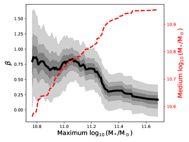
Figure 11: The change of the best-fit $\beta$ as more massive QGs are included to the fit (black solid line). The x-axis shows the maximum $M_{*}$ of the QGs included to the fit (see section 3.3 for details). The grey shaded regions mark the 0.5, 1 and 2$\sigma$ uncertainties. The red dashed line shows the medium $M_{*}$ of the QGs included to the fit.

Before we proceed to discuss the physical implications of the observed relationship between $R_{\rm{e}}$ and $z_{\rm{form}}$, we caution about two possibly important systematics. First, although the dependence on $M_{*}$ still remains, we find that the best-fit slope becomes flattened if we use the Continuity prior to reconstruct the non-parametric SFHs. Specifically, for the lower-mass ($\log_{10}M_{*}=10.3-11$) QGs $\beta$ changes from $\approx 0.8\pm 0.2$ (Dirichlet) to $\approx 0.5\pm 0.2$ (Continuity), and for the higher-mass ($\log_{10}M_{*}>11$) QGs it changes from $\approx 0.2\pm 0.1$ to $\approx 0.1\pm 0.1$. Second, the slope of the relation depends on which definition of formation redshift is adopted. Because the goal is to use SFHs to separate the progenitor effect from the late-time growth of galaxies, as we already discussed in the beginning of this section, the ideal choice then is $z_{\rm{form}}^{\rm{h}}$ which unfortunately is unknown. Using $z_{\rm{form}}$ thus is purely from an empirical stand point. Other proxies for $z_{\rm{form}}^{\rm{h}}$ are also considered, including the redshift $z_{\rm{form}}^{-0.5\tau_{\rm{tot}}}$ of lookback time ($t_{\rm{age}}$ $-$ $\tau_{\rm{tot}}$/2), and the redshift $z_{\rm{form}}^{-\tau_{\rm{SF}}}$ of lookback time ($t_{\rm{age}}$ $-$ $\tau_{\rm{SF}}$). No substantial changes to the best-fit relations are found. Quantitatively, the best-fit slope for the lower-mass QGs is $\beta=0.7\pm 0.2$ ($0.6\pm 0.2$) if $z_{\rm{form}}^{-\tau_{\rm{SF}}}$ ($z_{\rm{form}}^{-0.5\tau_{\rm{tot}}}$) is used. For the higher-mass QGs, the best-fit slope is $\beta=0.2\pm 0.1$ ($0.1\pm 0.1$) if $z_{\rm{form}}^{-\tau_{\rm{SF}}}$ ($z_{\rm{form}}^{-0.5\tau_{\rm{tot}}}$) is used.

We have also attempted to empirically evaluate the performances of individual proxies for $z_{\rm{form}}^{\rm{h}}$. In particular, assuming that the central regions of galaxies are much less affected by processes such as mergers relative to their outskirts, which in fact is supported by simulations of galaxy mergers (e.g. see Figure 3 in Hilz et al., 2013), we can compare the distributions of $\Sigma_{\rm{1kpc}}$ for galaxy samples selected to have formed at the same epoch, using different proxies for the formation redshift. If one proxy is better than others in separating the progenitor effect, then the galaxy sample selected using that proxy should have a narrower distribution of $\Sigma_{\rm{1kpc}}$. Perhaps because of the combination of relatively small sample size and large scatter (both intrinsic and introduced by our measures), however, we do not find any statistically significant difference among different proxies. This needs to be further investigated with larger samples in the future.

Setting aside the aforementioned systematics, for the lower-mass QGs the slope of the $R_{\rm{e}}$-$z_{\rm{form}}$ relation is always found to be steeper and closer to the value $\beta=1$ compared to the higher-mass QGs, regardless of which non-parametric SFH prior and proxy for formation redshift are used. This suggests that the progenitor effect becomes increasingly important in driving the apparent size evolution of QGs as they become less massive. In addition to $z_{\rm{form}}$, other characteristics of SFHs can also affect the apparent size evolution. As we already showed in section 3.1, galaxies can have very similar $z_{\rm{form}}$, yet, the timescale to assemble most of their mass can be dramatically different (Figure 8). In Figure 12, we further divide the lower-mass QG sample into two subsamples using $\tau_{\rm{tot}}$. The relatively small sample size and large scatter notwithstanding, two interesting things are noticed. Compared to the lower-mass QGs with larger $\tau_{\rm{tot}}$, we find likely evidence that those with smaller $\tau_{\rm{tot}}$ have a steeper evolution of $R_{\rm{e}}$ with $z_{\rm{form}}$. Meanwhile, at fixed $z_{\rm{form}}$, they also seemingly to have smaller $R_{\rm{e}}$. These suggest that the progenitor effect is more prominently observed in the lower-mass QGs with a more rapid and monolithic assembly history, as expected.

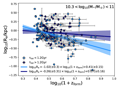
Figure 12: The relationship between $R_{\rm{e}}$ and $z_{\rm{form}}$ for the sample of lower-mass QGs. The galaxies are binned using the median value of $\tau_{\rm{tot}}$. The solid lines show the least squares linear regressions, and the light shaded regions show the 1$\sigma$ uncertainties. Best-fit relations and uncertainties are labelled in the figure legend.

For the higher-mass QGs, the relationship between $R_{\rm{e}}$ and $z_{\rm{form}}$ is in general nearly flat. A natural interpretation would be the increasing role that mechanisms of post-quenching size and mass growths play, i.e. from right after quenching to the time of observations. Note that this time lapse also tends to be larger for more massive galaxies, since these systems complete their formation and quenching at an earlier time (see Figure 9). One very plausible mechanism for such post-quenching growth is galaxy mergers, and minor mergers in particular. Assuming energy conservation of a merging system, as the distribution of orbital parameters in hydrodynamical simulations suggests that most merging halos are on parabolic orbits (Khochfar & Burkert, 2006), and using the Virial theorem, Naab et al. 2009 showed that minor mergers are much more efficient in growing galaxy sizes compared to major mergers, given a fixed amount of mass to be added to the central galaxy. Because the merger rate is expected to increase with stellar mass and redshift (e.g. Hopkins et al., 2010; Rodriguez-Gomez et al., 2015; O’Leary et al., 2021), galaxy mergers can effectively grow galaxy sizes by adding mass to the outskirts of compact QGs that formed relatively early. This scenario is also supported by the continuity analysis of the galaxy stellar-mass function, as discussed by Peng et al. (2010b), who argued that QGs with $M_{*}>10^{11}M_{\sun}$ should have significant growths in mass after the quenching, whilst a similar situation is very unlikely for lower-mass QGs. As we will discuss in section 3.4, our stacking analysis reaches similar conclusions, namely that the late-time size growth of very massive QGs is very likely driven by merging and accretion of small galaxies primarily to their outskirts. Finally, we have also verified that if we further divide the higher-mass QGs into subsamples using their $\tau_{\rm{tot}}$ we do not find statistically significant differences among the $R_{\rm{e}}$-$z_{\rm{form}}$ relationship as a function of $\tau_{\rm{tot}}$. This again suggests that, for these higher-mass QGs, by the time of observation, $z_{\rm{obs}}$, post-quenching size and mass growths have erased the memory of the structural properties that these massive galaxies had at $z_{\rm{form}}$, i.e. the time when they formed.

3.4 The Morphology of QGs in the Stacked HST Images

In this section, we further study the morphology of QGs by stacking their multi-band HST images. We pay particular attention to the low surface brightness flux which is too faint to be studied for individual QGs. HST bands included to the analysis are ACS/$I_{814}$, WFC3/$J_{125}$ and WFC3/$H_{160}$, because they are available in all three fields simultaneously. Motivated by the $M_{*}$ dependence of the relationship between $R_{\rm{e}}$ and $z_{\rm{form}}$ (Figure 10), the QGs are first divided into a lower-mass sample with $10^{10.3}M_{\sun}<M_{*}<10^{11}M_{\sun}$ and a higher-mass sample with $M_{*}>10^{11}M_{\sun}$. Each sample is then divided into three subsamples using the 3-quantiles of $z_{\rm{form}}$. These add up to 6 subsamples in total.

Before stacking, for each QG we first center on its SExtractor-derived light centroid in the $H_{160}$ band to make 10”$\times$10” cutouts of the HST images and the corresponding sigma maps. Each image is then rotated using the position angle in the $H_{160}$ band from van der Wel et al. (2012), which is measured by fitting the light profile with a single-Sérsic profile using Galfit. After this, the semi-major axis of all QGs is aligned along the North direction. We also use the segmentation map of the $H_{160}$ band provided by the CANDELS team to mask out any intervening objects detected in the cutouts. Finally, we stack the reprocessed images with inverse-variance weights.

3.4.1 Surface brightness profiles of the stacked QGs

Here we compare the multi-band surface brightness profiles of the stacked QGs. All stacked images are first PSF-matched to that of the $H_{160}$ band. Surface brightness profiles are then measured in the PSF-matched images using the elliptical annular apertures whose axis ratio (b/a) is fixed to the best-fit value in the $H_{160}$ band measured by Galfit assuming a single-Sérsic profile.

Two types of uncertainties are taken into account for the measurements. The first comes from sample random errors, which can be particularly important for the stacking analysis because sometimes a small number of galaxies can dominate the stacked signal. To quantify this uncertainty, each subsample has been bootstrapped 100 times. The other type of uncertainty comes from image noise. During each bootstrapping we thus use the corresponding stacked sigma map to Monte Carlo resample the pixel values of the stacked image 30 times with a normal distribution. We repeat the surface brightness measurements 100$\times$30$=$3000 times for each subsample and for each HST band. Finally, we use the range between 16th and 84th percentiles as 1$\sigma$ uncertainties of the surface brightness profiles.

In Figure 13 we show the stacked multi-band HST images and surface brightness profiles of every subsample. The stacking pushes the 1$\sigma$ detection limit of surface brightness to $\approx 29$ $\rm{mag/arcsec^{2}}$ in all three bands. For all subsamples the surface brightness in the $I_{814}$ band is much fainter than that in the $J_{125}$ and $H_{160}$ bands (see the inset of each panel), illustrating once again the effectiveness of the UVJ selection criteria in culling galaxies with very low levels of on-going star formation activity. We continue to compare the shape of surface brightness profiles by normalizing each profile with the central surface brightness. While the profile shapes of the $J_{125}$ and $H_{160}$ bands are very similar, we see evidence that the light in the $I_{814}$ band is more extended. Although the relatively small sample size prevents us putting the statistics on a solid ground at the moment, based on the uncertainties derived from our bootstrapping and Monte Carlo resampling, the finding that the light in the $I_{814}$ band is more extended than that in the $J_{125}$ and $H_{160}$ bands seems to be more prominent for the higher-mass QGs, particularly in the outer regions with $R_{maj}>0.5$ arcsec. This finding will soon be reinforced in section 3.4.2 via our single-Sérsic fitting analysis of the stacked images.

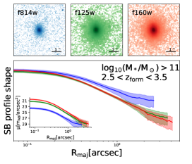
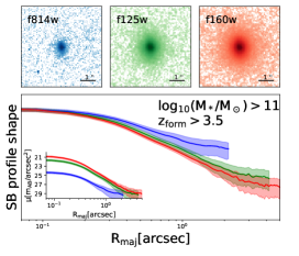
Figure 13: Surface brightness profile analysis for the stacked HST images of the six QG subsamples. In the panel of individual subsamples, the subpanels on the top show the three-band stacked HST images (PSF-unmatched). The shape of surface brightness profiles (in logarithmic scale) measured in the PSF-matched images are shown in the bottom subpanel, while the inset of it shows the surface brightness profiles in the physical unit of $\rm{mag/arcsec^{2}}$. The shaded region marks the 1$\sigma$ range of a measurement. Every surface brightness measurement stops at the radius corresponding to the 1$\sigma$ detection limit of the stacked image.

3.4.2 Single-Sérsic fitting results of the stacked QGs

Table 1: Single-Sérsic fitting results for the stacked HST images of individual subsamples.

$\rm{M_{*}/M_{\sun}}$	$\rm{z_{form}}$	$\rm{\#^{(a)}}$	$\rm{\langle z_{obs}\rangle^{(b)}}$	$\rm{{R_{e}^{F814W}}^{(c)}}$	$\rm{n^{F814W}}$	$\rm{{R_{e}^{F125W}}^{(c)}}$	$\rm{n^{F125W}}$	$\rm{{R_{e}^{F160W}}^{(c)}}$	$\rm{n^{F160W}}$
$10^{10.3}\sim 10^{11}$	$<1.9$	51	1.3	1.32$\pm$0.19	1.64$\pm$0.38	1.27$\pm$0.09	2.05$\pm$0.24	1.28$\pm$0.09	1.93$\pm$0.22
	$1.9\sim 2.5$	65	1.5	1.14$\pm$0.11	1.28$\pm$0.26	1.13$\pm$0.06	1.41$\pm$0.19	1.16$\pm$0.06	1.42$\pm$0.16
	$>2.5$	65	2.0	1.11$\pm$0.83	1.54$\pm$1.04	0.80$\pm$0.15	1.81$\pm$0.37	0.81$\pm$0.13	1.82$\pm$0.32
$>10^{11}$	$<2.5$	47	1.4	1.59$\pm$0.12	2.11$\pm$0.31	1.38$\pm$0.08	2.13$\pm$0.22	1.39$\pm$0.06	2.03$\pm$0.18
	$2.5\sim 3.5$	53	1.7	1.64$\pm$0.17	1.53$\pm$0.27	1.31$\pm$0.12	1.79$\pm$0.22	1.30$\pm$0.10	1.81$\pm$0.20
	$>3.5$	53	2.2	1.75$\pm$0.39	1.54$\pm$0.49	1.51$\pm$0.17	2.06$\pm$0.38	1.40$\pm$0.10	1.96$\pm$0.23

(a)– Total number of galaxies in the subsample; (b)– Median redshift of the subsample; (c)– In the unit of kpc.

We now study the morphology of individual stacked QG subsamples using Galfit. During the analysis, we adopt the PSFs produced by the CANDELS team and fit each stacked image with a 2-D Sérsic light profile, from which we obtain the Sérsic index $n$ and $R_{\rm{e}}$.

One complication of this analysis is to properly estimate the uncertainty of the fitted parameters. Similarly to what has already been described in section 3.4.1, both image noise and sample random errors are taken into account. We follow section 3.4.1 to estimate the uncertainty from the former by Monte Carlo resampling the image pixel values 30 times with the stacked sigma maps and the uncertainty from the latter by bootstrap resampling the stacked sample 100 times. We have compared the two uncertainties and found that sample random errors dominate over the uncertainty introduced by image noise. These add up to 3000 times Galfit fittings for each band and for each subsample. The Galfit single-Sérsic fitting results are tabulated in Table 1 and plotted in Figure 14.

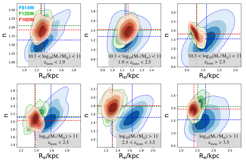
Figure 14: Single Sérsic fitting analysis with Galfit for the stacked HST images of the six QG subsamples. The contours show the distributions of best-fit $R_{\rm{e}}$ and $n$ derived from our Monte Carlo plus bootstrap resamplings (see section 3.4.2 for details). The dashed lines mark the medians.

To begin, we study the relationship between $z_{\rm{form}}$ and $R_{\rm{e}}$ ($H_{160}$) derived from the stacking where we use the median $z_{\rm{obs}}$ of individual subsamples to convert angular scales to physical scales. We show in Figure 15 the best-fit relations of the lower-mass (blue) and higher-mass (red) stacked QG samples. The stacking analysis confirms the $M_{*}$ dependence of the $R_{\rm{e}}$-$z_{\rm{form}}$ relationship as reported in section 3.3 based on individual QGs. The relation becomes shallower as the QGs become more massive. Quantitatively speaking, the best-fit values of $\beta$ derived from the stacking analysis are in great agreement ($\sim 0.5\sigma$ difference) with those derived from individual QGs. The best-fit intercept $C$ for the lower-mass QGs derived from the stacking seems to be larger than (though still within $\sim 1\sigma$ range) that derived from individual QGs (Figure 10). Interestingly, we find that this difference in $C$ disappears if we stack the images without pre-aligning the galaxies’ semi-major axis. Also noticed is that in all subsamples the best-fit Sérsic index $n$ is found to be $\sim 1.5-2$, while it becomes to $\sim 3-5$ when stacking without aligning the semi-major axis in advance. These suggest that the pre-alignment is critical in retrieving low surface brightness light on the outskirts. More importantly, these indicate that on average the morphology of high-redshift QGs, at least on their outskirts, is more disk-like rather than spheroidal, which is in agreement with recent morphological and dynamical studies of a few cases of $z\sim 2$ QGs where strong magnification by gravitational lensing helps reaching sub-kpc resolutions in the source plane (Newman et al., 2018b). We defer a detailed study on this finding and its implications on galaxy quenching to a forthcoming paper.

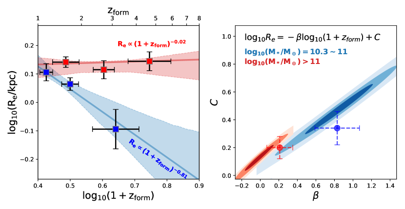
Figure 15: Left: The relationship between $R_{\rm{e}}$ and $z_{\rm{form}}$ derived from our stacking analysis (section 3.4.2). Blue shows the best-fit relation of the lower-mass QGs and red shows the best-fit relation of the higher-mass QGs. Right: The contours show the 0.5, 1 and 2$\sigma$ parameter uncertainties of the best-fit $R_{\rm{e}}$-$z_{\rm{form}}$ relation. Also marked using the circle with dashed error bars are the best-fit values and 1$\sigma$ uncertainties derived from individual QGs (see section 3.3 and Figure 10).

We finally compare the Sérsic fitting results in the $H_{160}$ band with the other two bluer HST bands, i.e. $I_{814}$ and $J_{125}$ (Figure 14). While the morphologies of the lower-mass QGs in all three bands are very similar, the higher-mass QGs have a more extended morphology, namely having large $R_{\rm{e}}$, in the $I_{814}$ band than in the $J_{125}$ and $H_{160}$ bands. These are consistent with the analysis of the surface brightness profiles in section 3.4.1. Together with the dependence of the relationship between $R_{\rm{e}}$ and $z_{\rm{form}}$ on $M_{*}$, the findings here are consistent with the picture that very massive QGs after they formed keep growing their sizes via merging with satellite star-forming galaxies, while for the lower-mass QGs, which presumably formed in the regions of lower overdensities compared to the higher-mass QGs, experienced much less mergers and (hence) their morphological properties still have the memory of the time when they formed.

3.5 The Relationship between the Compactness of QGs and Their Assembly History

We now study the relationships between the compactness of QGs and their SFH. While the results presented below are only about the relationships with $z_{\rm{form}}$, in Appendix E we also show the results of using other characteristic $z_{\rm{p}}$ where we find no substantial changes in any of our findings.

To begin, we present the relationships between stellar mass surface densities and $z_{\rm{form}}$ derived from the reconstructed SFHs (section 2.4). Figure 16 shows the results for $\Sigma_{\rm{1kpc}}$, and Figure 17 shows the results for $\Sigma_{e}$. On average, the QGs with larger stellar mass surface densities, regardless if measured within $R_{\rm{e}}$ or within the central radius of 1 kpc, tend to form earlier, i.e. have larger $z_{\rm{form}}$. This is broadly consistent with other studies (e.g. Tacchella et al., 2017; Williams et al., 2017) where compact QGs were found to have formed earlier compared to non-compact QGs. The majority of our QGs with $z_{\rm{form}}$ $>3$, meaning that they have assembled most of their mass within $<2$ Gyr since the Big Bang, have $\Sigma_{\rm{1kpc}}$ $\rm{>10^{10}\,M_{\sun}/kpc^{2}}$, being quantitatively consistent with the finding of Estrada-Carpenter et al. (2020).

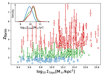
Figure 16: The relationship between $\Sigma_{\rm{1kpc}}$ and $z_{\rm{form}}$. Individual QGs are color-coded following $z_{\rm{form}}$ $<2$ (blue), $2<$$z_{\rm{form}}$ $<3$ (green) and $z_{\rm{form}}$ $>3$ (red). The density distributions of $\Sigma_{\rm{1kpc}}$ estimated using a Gaussian kernel are plotted in the inset.

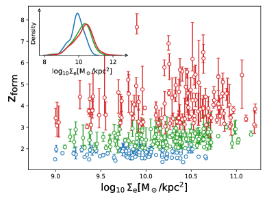
Figure 17: Similar to Figure 16, but for the relationship between $\Sigma_{e}$ and $z_{\rm{form}}$.

We continue by studying the relationship between $M_{\rm{1kpc}}/M_{*}$ and SFH. Because $M_{*}$, $\Sigma$ and $z_{\rm{form}}$ are inter-correlated with each other, making it very challenging to identify the real underlying physics driving the observed trend between $\Sigma$ and SFH, we use $M_{\rm{1kpc}}/M_{*}$ to mitigate the strong dependence of $\Sigma$ on $M_{*}$ (section 2.5, also see Ji et al. 2022 for more details) in order to have a more direct view on the relationship between galaxy morphology, specifically compactness and SFH. As Figure 18 shows, we find that the dependence of $z_{\rm{form}}$ on $M_{\rm{1kpc}}/M_{*}$ becomes much weaker than the dependence on $\Sigma$. This suggests that the increasing trend of $z_{\rm{form}}$ with $\Sigma_{e}$ and $\Sigma_{\rm{1kpc}}$ likely is just a reflection of the combined effect of the strong and positive correlation between $\Sigma$ and $M_{*}$ (e.g. Barro et al., 2017; Ji et al., 2022), and the increasing trend of $z_{\rm{form}}$ with $M_{*}$ (section 3.2).

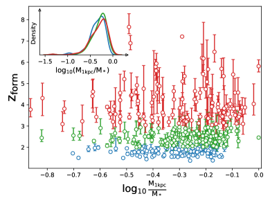
Figure 18: Similar to Figure 16, but for the relationship between $M_{\rm{1kpc}}/M_{*}$ and $z_{\rm{form}}$.

Motivated by the dependence of the relationship between $R_{\rm{e}}$ and $z_{\rm{form}}$ on $M_{*}$ (section 3.3 and 3.4), similarly to what we did in previous sections, we again divide the QGs into the lower-mass and higher-mass samples and study the relationships between the different metrics of galaxy compactness and $z_{\rm{form}}$. The $M_{*}$ dependence of the relationships is clearly seen in Figure 19. For the lower-mass QGs, we find the increasing trends of $z_{\rm{form}}$ with $\Sigma_{\rm{1kpc}}$, and with $\Sigma_{e}$. For the higher-mass QGs, however, the trends are essentially flat. We also find an increasing trend of $M_{\rm{1kpc}}/M_{*}$ with $z_{\rm{form}}$ for the lower-mass QGs, which is interesting given that no clear trend between $z_{\rm{form}}$ and $M_{\rm{1kpc}}/M_{*}$ was seen when QGs with all different stellar mass were mixed together (Figure 18). This shows the complication, likely introduced by the interplay between different physical processes, of the interpretation of the apparent (null) correlations. Qualitatively speaking, the findings here are fully in line with the picture that the progenitor effect becomes increasingly important as QGs become less massive, as it has already been discussed in section 3.3 when studying the size evolution. On the one hand, because the density of the Universe increases with redshift, this means that galaxies formed earlier also have larger densities. On the other hand, as is the case for very massive QGs, if significant late-time size growths take place after galaxies have formed and quenched, the morphological properties of galaxies can reduce the memory of the time of their formations, making the relationship between galaxy compactness and $z_{\rm{form}}$ flat. As will soon be discussed quantitatively in section 4.3, the increasing trends of $z_{\rm{form}}$ with $\Sigma_{\rm{1kpc}}$, $\Sigma_{e}$ and $M_{\rm{1kpc}}/M_{*}$ observed for the lower-mass QGs seemingly can be fully explained by the strong progenitor effect.

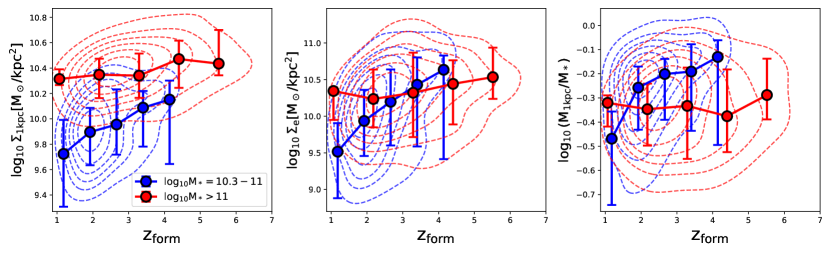
Figure 19: The relationships between $z_{\rm{form}}$ (horizontal axis) and galaxy compactness (vertical axis) for QGs with different $M_{*}$. Blue shows the results of the lower-mass QGs, and red shows the results of the higher-mass QGs. Contours show the density distributions estimated using a Gaussian kernel, while the circles with error bars show the median and 1$\sigma$ range of the compactness of QGs in individual $z_{\rm{form}}$ bins. From left to right the adopted compactness metrics are $\Sigma_{\rm{1kpc}}$, $\Sigma_{e}$ and $M_{\rm{1kpc}}/M_{*}$.

4 Discussions

To summarize, we utilized the fully Bayesian SED fitting code Prospector to reconstruct the non-parametric SFHs for a carefully culled sample of 361 massive QGs at $\langle$$z_{\rm{obs}}$ $\rangle\sim 2$ selected through the UVJ technique in the CANDELS/COSMOS and GOODS fields. The diverse assembly history is clearly seen in these high-redshift QGs. We have studied in detail the relationships between the evolution of the morphological properties of QGs and their assembly history. The relationships of $z_{\rm{form}}$ with $R_{\rm{e}}$, and with galaxy compactness ($\Sigma_{\rm{1kpc}}$, $\Sigma_{e}$ and $M_{\rm{1kpc}}/M_{*}$) show a clear dependence on stellar mass. All these findings converge to a general physical picture of the morphological evolution of QGs, namely that the progenitor effect plays a crucial role in the apparent evolution of the morphological properties of the QGs with $10.3<\log_{10}(M_{*}/M_{\sun})<11$, while the late-time size growths via galaxy mergers become increasingly important as QGs become more and more massive. In the following, we discuss the implications of our findings for the dynamical (section 4.1) and chemical (section 4.2) evolution of QGs. Finally, in section 4.3, we provide simple, empirical arguments that the progenitor effect alone can explain the apparent evolution of certain morphological properties of lower-mass QGs.

4.1 Implications for the dynamical evolution of QGs

The dependence of morphological evolution of QGs with $z_{\rm{form}}$ on $M_{*}$ could imply a similar $M_{*}$ dependence of dynamical evolution. On the one hand, among the more massive galaxies, those with lower $z_{\rm{form}}$ were born larger than those with higher $z_{\rm{form}}$, which were more compact at the time of formation. This implies that a substantial mass growth took place via mergers, which also grew the size of QGs with stellar mass $>10^{11}M_{\sun}$. This suggests that QGs at the high-mass end formed in dense environments, presumably in the regions with large overdensity of the primordial density field. Early on, these massive halos can gravitationally attract large amount of gas from surrounding cosmic webs. The gas is highly dissipative and thus can quickly sink to the center of gravitational potential, fueling intense star formation until the cumulative mass becomes so large that the infalling gas accreted later on are shock-heated by the halo potential (Dekel & Birnboim, 2006) which eventually leads to the quenching of star formation. After the formation, these very massive galaxies continue growing their sizes via merging with other galaxies through dynamic friction. We do not expect these galaxies to be fast rotators, since multiple incoherent merging episodes are expected to cause the loss of angular momentum (e.g Emsellem et al., 2011).

On the other hand, lower-mass QGs very likely formed in regions with comparatively smaller overdenties, meaning that they have shallower gravitational well and hence were not able to accrete gas from cosmic webs as efficiently as those galaxies in larger halos. As a result, lower-mass QGs may assemble in a much more slower and smoother manner. They may initially form as disks with high gas fractions, and then quench via secular processes like the bulge formations through the coalescence of star-forming clumps to the center of galaxies (Dekel et al., 2009). For these galaxies we expect to see significant rotations. Strong observational supports for the scenarios above come from the dynamical studies of Early Type Galaxies (ETGs) in the nearby Universe using ground-based Integral Field Unit spectroscopy. The distribution of the dynamical state of ETGs at $z\sim 0$ is bimodal, with one population dubbed “fast rotator” having much larger $v_{rot}/\sigma$ than the other one dubbed “slow rotator”. Interestingly, in the local universe fast and slow rotators can be very well separated using a characteristic $M_{*}=2\times 10^{11}M_{\sun}$, with the former being less massive (see a review by Cappellari 2016 and references therein). Therefore, our finding of the $M_{*}$ dependence of the morphological evolution of QGs at $z\sim 2$ seems to be quantitatively in line with the dynamical studies of ETGs at $z\sim 0$.

A critical test on the dynamical evolution is to directly measure the kinematics of high-redshift QGs. However, at high redshift, unlike star-forming galaxies whose dynamical properties can still be measured through strong emission lines either from ionized gas such as H$\alpha$ or from cold molecular gas such as CO, measuring the kinematics of QGs is very challenging because QGs have very low level of on-going star formation and very little molecular gas (e.g. Bezanson et al., 2019; Williams et al., 2021; Whitaker et al., 2021), and they are very compact. The robust dynamical measurements of QGs thus require deep and spatially-resolved spectroscopy at the rest-frame optical wavelengths where abundant stellar absorption features exist. Substantial progress has been recently made in understanding the kinematics of QGs at $0.5<z<1$ (e.g. Bezanson et al., 2018b). At $z\sim 2$ and beyond, while current instrumentation only allows such measurements for a few cases of gravitationally lensed QGs (Toft et al., 2017; Newman et al., 2018a), the upcoming JWST should significantly improve this situation.

4.2 Implications for the chemical evolution of QGs

The chemical composition of galaxies is another key parameter to constrain the physics of formation and evolution of QGs across cosmic time. The dependence of morphological evolution on $M_{*}$ could also imply the $M_{*}$ dependence of the evolution of chemical properties of QGs. Without strong nebular emission lines, the only probe of the chemical properties of QGs is stellar absorption features which require ultradeep NIR spectroscopy with current ground-based 10m telescopes. Some progress has been made recently in measuring the chemical compositions of a handful of QGs at $z>1$ using either individual spectra (Lonoce et al., 2015; Kriek et al., 2019; Lonoce et al., 2020) or stacked spectra (Onodera et al., 2015). Some intriguing, but not yet conclusive, results have already been found. For example, Kriek et al. (2019) successfully measured the abundance ratios [Mg/Fe] and [Fe/H] in three massive ($\log_{10}M_{*}\sim 11$) QGs at $z\sim 1.4$, where they found tentative evidence that (1) while the relationships between [Mg/Fe] and $M_{*}$ are consistent at $z\sim 1.4$ and at $z<0.7$, [Fe/H] is lower at $z\sim 1.4$ than at $z<0.7$; and (2) relative to QGs at $z\sim 0$, the offset of [Mg/Fe] of massive QGs decreases with redshift. Taken together, this evidence suggests that high-redshift massive QGs need to accrete low-mass and less $\alpha$-element enhanced galaxies to explain the observations. We also highlight another work from Jafariyazani et al. (2020) where for the first time they were able to measure abundance ratios of other six elements (apart from Mg and Fe) and their radial gradients inside a very massive QG ($\log_{10}M_{*}\sim 11.7$) at $z=1.98$ thanks to the magnification effect of strong gravitational lensing. This QG was found to be not only Mg-enhanced but also Fe-enhanced compared to the center of nearby ETGs. If this QG is a typical progenitor of ETGs at $z\sim 0$, the findings then suggest that significant radial mixing of stars with different chemical abundances have to take place inside very massive QGs, even in their central regions.

Despite the very small sample size of existing measurements of chemical compositions of QGs at $z>1$, all studies seem to consistently suggest that processes like galaxy mergers are needed to explain the chemical evolution of QGs with $\log_{10}M_{*}>11$, which is fully in line with our conclusions based upon the morphological evolution of QGs. Future JWST observations will not only significantly enlarge the number of chemical measurements of very massive QGs at high redshift, but also push the measurements to lower masses and eventually enable testing if the chemical evolution of QGs also depends on stellar mass.

4.3 Can the progenitor effect alone explain the observed relationships between galaxy compactness and $z_{\rm{form}}$ for the lower-mass QGs?

Setting aside the potential systematic errors from the assumed prior of non-parametric SFHs and the proxy used for $z_{\rm{form}}^{\rm{h}}$, which we discussed in detail in section 3.3, for the lower-mass QGs ($10.3<\log_{10}(M_{*}/M_{\sun})<11$) the slope of the relationship between $R_{\rm{e}}$ and $z_{\rm{form}}$ is consistent with the value $-1$. This can be fully explained in terms of the formation of dark matter halos, indicating that the progenitor effect plays a predominant role in the apparent size evolution of the lower-mass QGs. Obviously, this means that the progenitor effect should also play an important role in the apparent evolution of QGs’ compactness because all compactness metrics discussed in section 3.5 directly depend on $R_{\rm{e}}$. An important question yet to be answered is, can the progenitor effect alone be enough to explain the apparent evolution of compactness of lower-mass QGs? The answer is critical for understanding not only if there are additional physical links between galaxy compactness and $z_{\rm{form}}$, but also if there is a causal link between galaxy compactness and quenching.

To begin, we test the progenitor effect on the apparent evolution of stellar mass surface densities. We introduce a purely empirical but physically motivated parameter, comoving stellar mass surface density, which is defined as

$$\rm{comoving\mbox{-}\Sigma=\frac{\Sigma}{(1+z_{\rm{form}})^{2}}}$$ (10)

The reason of normalizing $\Sigma$ with $z_{\rm{form}}$, rather than $z_{\rm{obs}}$, has already been explained in section 3.3, namely that the morphological properties (e.g. density) of galaxies should reflect the earlier time when they formed, if the progenitor effect is strong which is the case for the lower-mass QGs based on the $z_{\rm{form}}$-$R_{\rm{e}}$ relationship. The left two panels of Figure 20 show the relationships between $z_{\rm{form}}$ and comoving-$\Sigma_{\rm{1kpc}}$, and between $z_{\rm{form}}$ and comoving-$\Sigma_{e}$, respectively. For comparison, we also show the relationships of $\Sigma_{\rm{1kpc}}$ and $\Sigma_{e}$ in light blue. It is clear that the evolution becomes very weak, if any, once stellar mass surface densities are normalized by the cosmic density at $z_{\rm{form}}$, suggesting that the progenitor effect alone is largely sufficient to explain the apparent correlations between $z_{\rm{form}}$ and $\Sigma$.

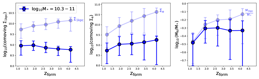
Figure 20: Empirical tests of the progenitor effect on the apparent morphological evolution of the lower-mass QGs. From left to right show the relationships of $z_{\rm{form}}$ with comoving-$\Sigma_{\rm{1kpc}}$, comoving-$\Sigma_{e}$ and $M_{\rm{R}}/M_{*}$ (see section 4.3 for details). For comparison, we also use light blue to plot the relationships already shown in Figure 19 for the lower-mass QGs.

We stress however that, depending on the radius within which $\Sigma$ is measured, the characteristic redshift used for the normalization should, strictly speaking, corresponds to the exact epoch when the regions within that radius assembled. This needs the knowledge not only of the galaxies’ integrated assembly history but also that of their sub-structures, for example the central regions and the outskirts. This requires the reconstruction of spatially resolved SFH which unfortunately is not currently feasible for high-redshift QGs. We argue, however, that using $z_{\rm{form}}$ to normalize stellar mass surface densities, both for comoving-$\Sigma_{\rm{1kpc}}$ and comoving-$\Sigma_{e}$, provides a reasonable substitute, as we explain in what follows.

The mass assembly of galaxies is not self-similar, namely some parts (e.g. bulge) form earlier while others (e.g. disk) form later. Studies of the growth of massive star-forming galaxies at $z>1$ consistently show that massive galaxies grew their inner regions earlier (e.g. Nelson et al., 2012, 2016; Tacchella et al., 2017). Despite being crude, it is therefore not unreasonable for us to assume that high-redshift QGs assembled their mass in a strictly inside-out manner. Under this assumption, $z_{\rm{p}}$ derived from the reconstructed SFHs then is the epoch when the central region within the radius containing p-percent total stellar mass has assembled. The redshift used for the normalization of $\Sigma_{e}$ thus should be either $z_{50}$ or $z_{\rm{form}}$. We have checked that the results of using the two redshifts are essentially identical. Similarly, the redshift used for the normalization of $\Sigma_{\rm{1kpc}}$ should be $z_{\rm{p}}$ where p equals to the fractional mass within the central 1kpc, i.e. $M_{\rm{1kpc}}/M_{*}$. Because the median $M_{\rm{1kpc}}/M_{*}$ of the sample of lower-mass QGs is $\approx 0.5$ (0.59$\pm$0.18, Figure 18), using $z_{\rm{form}}$ for comoving-$\Sigma_{\rm{1kpc}}$ therefore is also reasonable. We have also tested our results by normalizing $\Sigma_{\rm{1kpc}}$ using the $z_{\rm{p}}$ determined by $M_{\rm{1kpc}}/M_{*}$ for individual QGs, where no substantial changes were found. To this end, we believe that our empirical approach of normalizing galaxy compactness metrics with $z_{\rm{form}}$ in general should be able to capture the progenitor effect imprinted on the apparent evolution of galaxy compactness of our lower-mass QG sample.

We finally discuss the apparent evolution of $M_{\rm{1kpc}}/M_{*}$. Because galaxies formed earlier tend to have smaller $R_{\rm{e}}$, and meantime $M_{\rm{1kpc}}/M_{*}$ is measured using the fixed central 1 kpc no matter what $z_{\rm{form}}$ a galaxy has, these mean that the 1 kpc scale probes a relatively larger area for galaxies having larger $z_{\rm{form}}$ than those having smaller $z_{\rm{form}}$. This is how the progenitor effect enters in the apparent evolution of $M_{\rm{1kpc}}/M_{*}$. To quantify its contribution, we modify $M_{\rm{1kpc}}/M_{*}$ (equation 7) to $M_{\rm{R}}/M_{*}$ where, instead of using the fixed 1 kpc, for individual galaxies we adopt

$$R=1\,\rm{kpc}\cdot\frac{1+z_{\rm{form}}^{\rm{min}}}{1+z_{\rm{form}}}$$ (11)

and $z_{\rm{form}}^{\rm{min}}$ is the minimum $z_{\rm{form}}$ of the sample. As the right-most panel of Figure 20 shows, the increasing trend of $M_{\rm{1kpc}}/M_{*}$ with $z_{\rm{form}}$ almost disappears after using $M_{\rm{R}}/M_{*}$, suggesting that the key driver of the apparent correlation between $z_{\rm{form}}$ and $M_{\rm{1kpc}}/M_{*}$ is the progenitor effect.

5 Summary

This is the first of a series of papers that aim to investigate the relationships between the star-formation and structural properties of galaxies and their assembly history at the Cosmic Noon epoch. In this work, we focus on a sample of UVJ-selected massive quiescent galaxies (QGs) with stellar mass $M_{*}>10^{10.3}M_{\sun}$ and at a median redshift $\langle z_{\rm{obs}}\rangle\approx 1.9$ in the CANDELS/COSMOS and GOODS fields (section 2.1). Thanks to the accumulated high-quality panchromatic photometry that densely samples the rest-frame UV-Optical-NIR spectra of the galaxies (section 2.2), we utilize the fully Bayesian SED fitting code Prospector to reconstruct the SFH of QGs (section 2.3 and 2.4) and find a broad diversity among their assembly histories (section 3.1).

Following Lilly & Carollo (2016), we refer to the dependence of properties of galaxies observed at $z_{\rm{obs}}$ on $z_{\rm{form}}$, the time of formations defined as the redshift when a galaxy has assembled half of the mass it has at $z_{\rm{obs}}$, as the progenitor effect. The key finding of this paper is that the progenitor effect is important, and if not accounted for, it introduces spurious correlations between galaxies’ observables. Specifically,

• We have studied the progenitor effect in terms of the relationship between the half-light radius $R_{\rm{e}}$ measured at $z_{\rm{obs}}$, and $z_{\rm{form}}$ (section 3.3). We have quantified the relationship with the form $R_{e}\propto(1+z_{\rm{form}})^{-\beta}$. We have found that the relationship becomes steeper, i.e. having larger $\beta$, as QGs become less massive. This dependence on stellar mass has been further confirmed by our stacking analysis (section 3.4).

• Regardless of the systematics introduced by the specific prior assumed during the non-parametric SFH reconstructions, which appear to be relatively minor, and the usage of $z_{\rm{form}}$ (section 3.3), using our fiducial SED modeling which has been validated with the IllustrisTNG simulations (Appendix A), we have found that, for lower-mass QGs with $10.3<\log_{10}M_{*}<11$, the relationship is consistent with $R_{e}\propto(1+z_{\rm{form}})^{-1}$, namely what is expected if the central density of the galaxies keeps memory of the value it had at the initial collapse, suggesting that, after quenching, merging and interactions had a minimal influence in continue shaping the central light (and thus, mass) profile.

  For higher-mass QGs with $\log_{10}M_{*}>11$ the relationship flattens, tending towards the value $\beta=0.2\pm 0.1$. This suggests that for very massive galaxies, after quenching, the light profile continues to evolve and converges to a constant shape, which is typical of relaxed structures. In turn, this suggests that merging played a substantial role. We have also stacked the multi-band HST images for the QGs. Evidence that the higher-mass QGs have a more extended light profile in the $I_{814}$ band than in the $J_{125}$ and $H_{160}$ bands, based on both the analysis of surface brightness profiles and the analysis of single-Sérsic fittings with Galfit, has been found, suggesting that after-quenching growths of massive galaxies are due to merging satellite star-forming galaxies.

  We have also highlighted that the mass value $\log_{10}M_{*}\approx 11$, which separates the two post-quenching evolutionary regimes, is essentially the same as the one that separates fast rotators from slow rotators in local ETGs, suggesting a direct evolutionary link with the populations of $z\sim 2$ QG.

• Similar to the stellar-mass dependence observed for the relationship between $R_{\rm{e}}$ and $z_{\rm{form}}$, the relationship between the compactness of QGs and $z_{\rm{form}}$ also depends on stellar mass (section 3.5). Increasing trends of $z_{\rm{form}}$ are found with $\Sigma_{\rm{1kpc}}$, $\Sigma_{e}$ and $M_{\rm{1kpc}}/M_{*}$ for the lower-mass QGs, while they become very flat for the higher-mass QGs.

  We have empirically evaluated the progenitor effect on the apparent trend between compactness and $z_{\rm{form}}$ for the lower-mass QGs by introducing the “comoving” central surface mass density of galaxies (comoving-$\Sigma$), which is the central surface mass density normalized by the cosmic density at the time of their formations. Unlike what we found for $\Sigma$, comoving-$\Sigma$ does not depend on $z_{\rm{form}}$, meaning that the larger central stellar density and compactness of the lower-mass QGs at higher redshift can be fully explained by the progenitor effect, without requiring any additional physical mechanisms.

As a concluding remark, finally, we observe that this work highlights the importance, and the effectiveness, of measuring the SFH of galaxies before attempting any inference into their evolution from observed correlations of properties at any given epoch. Our tests, as well as those done by others (e.g. Leja et al., 2019a; Tacchella et al., 2022), conducted using cosmological simulations show that the Prospector code appears capable to robustly reconstruct the SFH of galaxies at $z=1-7$ with sufficient precision and accuracy to unveil trends of galaxy properties, when good-quality and densely sampled panchromatic photometry and/or spectroscopy is available. The reconstruction of SFHs by SED modeling seems to be leaving its infancy and enter a phase where it can be used as a power tool of investigation of galaxy evolution.

6 ACKNOWLEDGMENT

We thank the anonymous referee for useful comments. We are indebted to Alvio Renzini for illuminating discussions and for his comments on an earlier version of the manuscript. We thank Joel Leja for his generosity in providing us with advice and guidance on running Prospector. This work was completed in part with resources provided by the University of Massachusetts’ Green High Performance Computing Cluster (GHPCC).

Appendix A Validation of the Prospector fitting procedure with the IllustrisTNG simulations

We test the robustness of our Prospector SED fitting procedure using the IllustrisTNG simulations. In particular, we use the results from the run TNG100-3 for this validation and choose the simulation snapshot (#33) corresponding to $z=2$, i.e. about the median redshift ($\langle z\rangle=1.9$) of our QGs sample, for the TNG sample selection. As the left panel of Figure 21 shows, we select the sample of TNG QGs using the “main sequence” diagram, i.e. sSFR vs. $M_{*}$. Because the focus of this study is on massive galaxies, we only look at $M_{*}\geq 10^{10}M_{\sun}$ TNG galaxies and select those with $\rm{sSFR\leq 10^{-10}yr^{-1}}$ as our TNG QGs sample (marked with red squares in the Figure). These give us a sample with 72 simulated QGs. We then use the TNG’s “SubLink” halo merger tree to extract the full assembly histories for individual galaxies, which are then used to generate synthetic spectra with the stellar population synthetic code Fsps-v3.0 (Conroy et al., 2009; Conroy & Gunn, 2010). For each synthetic spectrum, we assume the Kroupa 2001 initial mass function, Byler et al. 2017 nebular emission (line+continuum) model, Calzetti et al. 2000 dust attenuation law with the fixed color excess $\rm{E(B-V)=0.2}$ that has been observed in typical early type galaxies (e.g. Domínguez Sánchez et al., 2011), and the stellar metallicity value that equals to the value of individual galaxies at the Snapshot#33 (i.e. we ignore the evolution of metallicity during galaxy assemblies). In other words, we adopt the same assumptions we have made to run Prospector when fitting the SED of the real galaxies. With the synthetic spectra in hand, we then convolve them with the filter throughputs in the GOODS-South field (note that the CANDELS/COSMOS and GOODS-North have a very similar set). To model the data quality of observations, we assign the flux uncertainty in each filter according to the median observed SNR of our sample (Figure 22).

Using the Dirichlet prior, we fit the synthetic data with the exactly same setup as described in section 2.3. The comparisons between the true SFHs and the Prospector-recovered SFHs are shown in the right panels of Figure 21. Our fitting procedure is able to reconstruct galaxy assembly histories to a great extent. More quantitative comparisons are shown in the first row of Figure 23, where the recovered mass-weighted age, $z_{50}$, $z_{70}$ and $z_{90}$ are plotted against the true values. In all cases, using the Dirichlet prior results in robust measures of the SFHs for the TNG QGs. Also needed to point out is that, despite that we only have the photometric data hence we do not expect to have strong constrains on galaxy stellar metallicity, the deviation of the recovered SFH parameters from the true values does not correlate with the assumed metallicities, suggesting that the not well-contrained metallicity cannot lead to significant errors of the reconstructed SFHs.

Figure 21: Left: The sample selection of TNG QGs. The selection is done with the Illustris-TNG100-3 run and at its Snapshot#33 corresponding to $z=2$. Galaxies marked with red squares are selected as our TNG QGs sample for the SED fitting robustness tests. Right: The upper panel shows the distribution of mass-weighted age for the TNG QGs sample. The vertical red solid line marks the median. The whole sample is divided into two groups, the younger one with mass-weighted ages less than the median and the old one larger than the median. The bottom panels show the comparison between true SFHs and recovered SFHs using the Dirichlet prior, with the younger group shown on the left and the old one shown on the right. The thick red dashed line and the red shaded region show the median and 16th-84th percentile range of the true SFHs, while the black step plots with solid and dashed line styles show the recovered median and 16th-84th percentile range of SFHs.

Figure 22: Observed signal-to-noise ratio (SNR) of each photometric band in the CANDELS/GOODS-South. From left to right show the bands from blue to red. Circles are the medians, while the error bars are the 16th-84th percentile ranges.

In addition to the Dirichlet prior, we have also run Prospector for the TNG QGs using the Continuity prior, which models changes of SFR in adjacent time bins by means of the variate $\rm{x=log(SFR_{t_{i}}/SFR_{t_{i+1}})}$ and, importantly, strongly disfavours sharp changes of x. We refer readers to Leja et al. (2019a) for the details of the model, but, briefly, the prior in the Continuity non-parametric SFH is assumed to be a Student’s-t distribution $\rm{P(x,\nu,\sigma)}$, where $\sigma$ controls the width of distribution and $\nu$ is the number of degrees of freedom that controls the tail of the distribution. Calibrated using $\approx 30,000$ galaxies with $M_{*}\geq 10^{9}M_{\sun}$ at $z=0$ (the vast majority are star-forming galaxies) from the Illustris simulations (Vogelsberger et al., 2014), Leja et al. 2019a suggested $\sigma=0.3$ and $\nu=2$ which are used here. We used the Continuity prior to fit the synthetic galaxies and compared the recovered SFHs with the true ones, using the same procedures adopted for the Dirichlet prior. As the second row of Figure 23 shows, while strong correlations between parameters related to the recovered and the true SFH are observed overall, systematic offsets exist. Specifically, compared with the Dirichlet prior (the third row of Figure 23), the Continuity prior in general over-estimates the mass-weighted age by $\approx 0.5$ Gyr. It also over-estimates $z_{50}$, $z_{70}$ and $z_{90}$. These findings are consistent with what reported by Leja et al. (2019a) for galaxies with the “Sudden Quench” SFHs (see the right-most column of their Figure 5). Also noticed from the third row of Figure 23 is the fact that the dispersion of the measurements is larger when the Continuity prior is used, again showing that the Dirichlet prior generally works better for the TNG QGs.

The reason behind the over-estimation of stellar ages of the TNG QGs with the Continuity prior can be clearly seen in Figure 24. Because the Continuity prior strongly opposes sharp changes in SFR, the reconstructed SFHs are forced to be smooth. Specifically, rather than putting more mass in fewer time bins, the Continuity prior tends to disperse the mass into more time bins. This is particularly seen in the old time bins because young and bright stars outshine older stars in the rest-frame optical-NIR, meaning that the goodness-of-fit does not change too much when slightly altering the SFH of the older stellar populations (Papovich et al., 2001) given the data coverage. The similar was also found in Johnson et al. (2021) (see the bottom panel of their Figure 3). However, because the TNG QGs indeed show very sudden changes in SFRs at early epochs (i.e. old time bins), this leads to the obvious mismatch between the assumption of the Continuity prior and the true shape of SFHs of the TNG QGs, and consequentially the discrepancies between the recovered and the true SFHs.

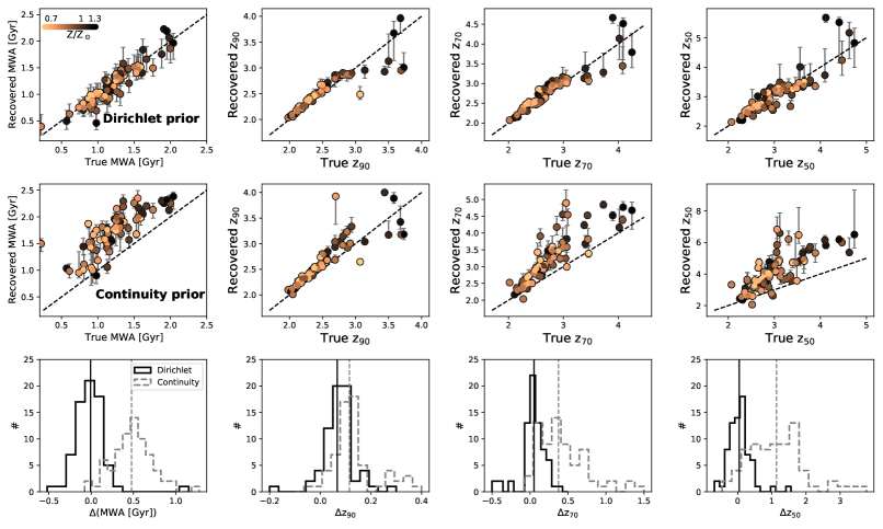
Figure 23: Comparisons between the recovered SFH-related parameters and the true values. The 1st row: The comparisons for the measurements assuming the Dirichlet prior. From left to right show the results of mass-weighted age, $z_{90}$, $z_{70}$ and $z_{50}$. Each galaxy is color-coded with its metallicity. The black dashed line shows the one-to-one relation. The 2nd row: The comparisons for the measurements assuming the Continuity prior. The 3rd row: The distributions for the deviations of the measurements from the true values. Black histograms are for the Dirichlet prior, the grey ones are for the Continuity prior. Also marked in each histogram as vertical lines are the medians.

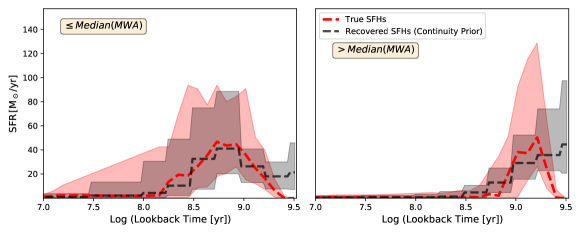
Figure 24: Similar to the bottom-right two panels of Figure 21, but we now compare the true SFHs with the recovered SFHs assuming the Continuity prior. The left panel shows the results for the younger TNG QGs, i.e. those have mass-weighted ages less than the median value of the whole TNG QGs sample, while the right panel shows the results for the older TNG QGs.

We conclude that our Prospector SED fitting procedure with the Dirichlet prior can robustly recover the assembly histories for the TNG QGs. Our tests also put in evidence the footprint of the assumed priors on the SFH reconstruction. While the Continuity prior may be a very good choice for star-forming galaxies, it is not as good as the Dirichlet prior for the QGs. However, we stress the limitations of our test with the TNG simulations. First and foremost, our conclusion on the best prior to use with non-parametric SFHs relies on the assumptions that 1) any difference between the SFHs of simulated TNG QGs and the real ones, regardless of how correctly the former capture the latter, does not affect the performance of Prospector in carrying out the reconstruction of the SFH itself, and 2) the systematic error from the mismatch between the real stellar populations at high redshift and the synthesis model (Fsps here) used to generate synthetic photometry for the TNG QGs is minor. Second, we emphasize that we are not making the statement that the Continuity prior should not be used for the QGs. Recall that the Student’s distribution used by the Continuity prior is governed by $\sigma$ and $\nu$. As already mentioned above, the values used here are from the calibration with the Illustris simulations at $z=0$ where the vast majority of the sample are star-forming galaxies. It is entirely plausible that, if we re-calibrate $\sigma$ and $\nu$ using QGs, the Continuity prior may still work well. Such calibration is beyond the scope of this work. The fact that using the Dirichlet prior can reproduce the overall shapes of true SFHs, and quantitatively recover the true values of parameters including mass-weighted age, $z_{50}$, $z_{70}$ and $z_{90}$, makes us believe our reconstructed SFHs of the QGs are statistically robust.

Appendix B Physical parameters derived with the Continuity prior for the sample QGs

While tests with simulations provide very valuable guidance to assess the performance of the SED fitting procedure, considering the limitations that we detailed in the end of Appendix A, we decide to additionally do an empirical test, namely to run a new set of Prospector fittings with the Continuity prior for our sample QGs (section 2.1), to check if any significant systematic error introduced by the prior could exist in the measures. In any case, as the direct comparison of key parameters obtained using the two priors illustrates (see Figure 25), the strong correlations between the two sets of measurements are seen, meaning that switching from the Dirichlet prior to the Continuity one will not qualitatively change any conclusion of this work.

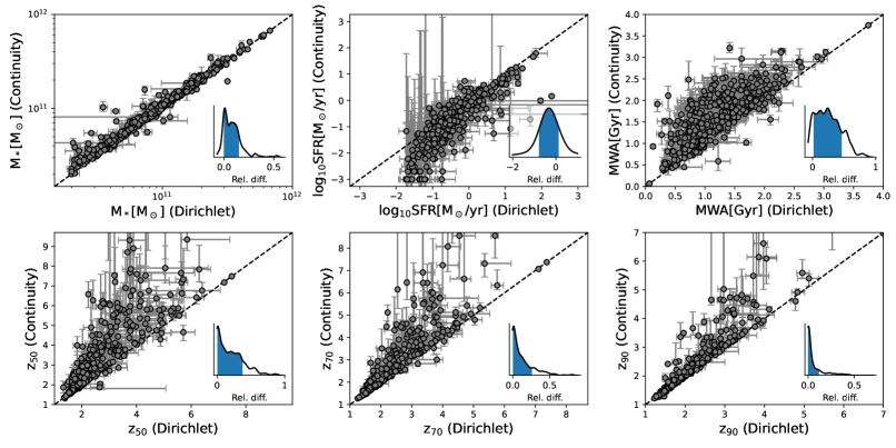
Figure 25: Comparisons of physical parameters derived using different priors of non-parametric SFHs for our sample QGs (section 2.1). The y-axis shows the measurements using the Continuity prior, and the x-axis shows the measurements using the Dirichlet prior. The black dashed line marks the one-to-one relation. The inset of each panel shows the distribution of relative differences, i.e. (y-x)/y, between the two measurements where the 1$\sigma$ range is filled with blue.

Appendix C Physical parameters derived by fixing metallicity during the SED fitting

We also empirically test that if our results are sensitive to the assumption on metallicity during the SED fitting. Unlike Appendix B where the entire sample was used, here we only use the sample from the GOODS-South field for the test. We run a new set of SED fittings using the same assumptions as our fiducial model (Dirichlet) except that metallicity is fixed to the solar metallicity during the fittings. We compare the measurements in Figure 26. Compared to the systematic errors introduced by the priors (Figure 25), the errors introduced by the assumptions on metallicity are much smaller, and they cannot change any conclusion of this work.

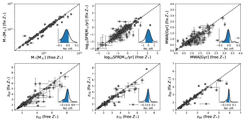
Figure 26: Similar to Figure 25, but for the comparisons of physical parameters derived by fixing (y-axis) or freeing (x-axis) metallicity during the SED fitting.

Appendix D Comparing the Skewness of SFHs with $\tau_{\rm{SF}}$/$\tau_{\rm{Q}}$

In section 2.4, we introduced two ways to characterize the asymmetry of SFHs, namely the Skewness and $\tau_{\rm{SF}}$/$\tau_{\rm{Q}}$. We compare them in the left panel of Figure 27 where we see great agreement between the two metrics. We also find some outliers where clear discrepancies exist between the two metrics. In the right panel of the Figure, we plot SFHs of the individual outliers. We immediately see the complex shape of SFHs of the outliers, showing the reason of the discrepancies between the Skewness and $\tau_{\rm{SF}}$/$\tau_{\rm{Q}}$.

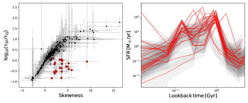
Figure 27: Left: The comparison between the Skewness of SFHs and $\tau_{\rm{SF}}$/$\tau_{\rm{Q}}$ (see the definitions in section 2.4). The two metrics describing the asymmetry of SFHs agree with other other very well, except some outliers which are labelled with red squares. Right: SFHs of the individual outliers.

Appendix E The relationships between stellar mass, mass surface density and $z_{\rm{p}}$

In the main text we presented the relationships between stellar mass and $z_{\rm{form}}$ (section 3.2), and between galaxy compactness and $z_{\rm{form}}$ (section 3.5). Here, instead of using $z_{\rm{form}}$, in Figure 28 and 29 we test the relationships using other characteristic $z_{\rm{p}}$ that we defined in section 2.4.

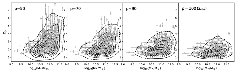
Figure 28: Similar to Figure 9, but instead of using $z_{\rm{form}}$, we show the relationships of $M_{*}$ with other characteristic redshifts $z_{\rm{p}}$, i.e. the redshifts when the p-percentage of $M_{*}$ has already formed. The dashed contours show the density distributions estimated using a Gaussian kernel.

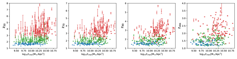
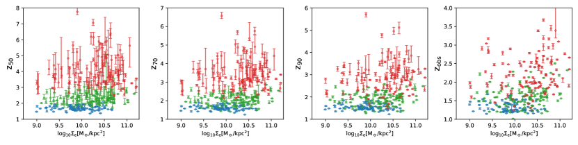
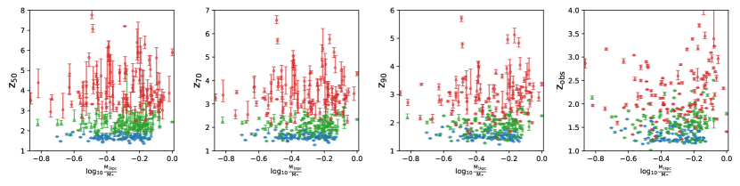
Figure 29: Similar to Figure 16, 17 and 18, but instead of using $z_{\rm{form}}$, we show the relationships of $\Sigma_{\rm{1kpc}}$ (the first row), $\Sigma_{e}$ (the second row) and $M_{\rm{1kpc}}/M_{*}$ (the third row) with other characteristic redshifts, namely $z_{50}$, $z_{70}$, $z_{90}$ and $z_{\rm{obs}}$.

References

- Barro et al. (2013) Barro, G., Faber, S. M., Pérez-González, P. G., et al. 2013, ApJ, 765, 104, doi: 10.1088/0004-637X/765/2/104
- Barro et al. (2017) Barro, G., Faber, S. M., Koo, D. C., et al. 2017, ApJ, 840, 47, doi: 10.3847/1538-4357/aa6b05
- Barro et al. (2019) Barro, G., Pérez-González, P. G., Cava, A., et al. 2019, ApJS, 243, 22, doi: 10.3847/1538-4365/ab23f2
- Belli et al. (2019) Belli, S., Newman, A. B., & Ellis, R. S. 2019, ApJ, 874, 17, doi: 10.3847/1538-4357/ab07af
- Bertin & Arnouts (1996) Bertin, E., & Arnouts, S. 1996, A&AS, 117, 393, doi: 10.1051/aas:1996164
- Bezanson et al. (2019) Bezanson, R., Spilker, J., Williams, C. C., et al. 2019, ApJ, 873, L19, doi: 10.3847/2041-8213/ab0c9c
- Bezanson et al. (2009) Bezanson, R., van Dokkum, P. G., Tal, T., et al. 2009, ApJ, 697, 1290, doi: 10.1088/0004-637X/697/2/1290
- Bezanson et al. (2018a) Bezanson, R., van der Wel, A., Straatman, C., et al. 2018a, ApJ, 868, L36, doi: 10.3847/2041-8213/aaf16b
- Bezanson et al. (2018b) Bezanson, R., van der Wel, A., Pacifici, C., et al. 2018b, ApJ, 858, 60, doi: 10.3847/1538-4357/aabc55
- Buitrago et al. (2008) Buitrago, F., Trujillo, I., Conselice, C. J., et al. 2008, ApJ, 687, L61, doi: 10.1086/592836
- Bundy et al. (2010) Bundy, K., Scarlata, C., Carollo, C. M., et al. 2010, ApJ, 719, 1969, doi: 10.1088/0004-637X/719/2/1969
- Byler et al. (2017) Byler, N., Dalcanton, J. J., Conroy, C., & Johnson, B. D. 2017, ApJ, 840, 44, doi: 10.3847/1538-4357/aa6c66
- Calzetti et al. (2000) Calzetti, D., Armus, L., Bohlin, R. C., et al. 2000, ApJ, 533, 682, doi: 10.1086/308692
- Cappellari (2016) Cappellari, M. 2016, ARA&A, 54, 597, doi: 10.1146/annurev-astro-082214-122432
- Cardamone et al. (2010) Cardamone, C. N., van Dokkum, P. G., Urry, C. M., et al. 2010, ApJS, 189, 270, doi: 10.1088/0067-0049/189/2/270
- Carnall et al. (2019a) Carnall, A. C., Leja, J., Johnson, B. D., et al. 2019a, ApJ, 873, 44, doi: 10.3847/1538-4357/ab04a2
- Carnall et al. (2018) Carnall, A. C., McLure, R. J., Dunlop, J. S., & Davé, R. 2018, MNRAS, 480, 4379, doi: 10.1093/mnras/sty2169
- Carnall et al. (2019b) Carnall, A. C., McLure, R. J., Dunlop, J. S., et al. 2019b, MNRAS, 490, 417, doi: 10.1093/mnras/stz2544
- Carollo et al. (2013) Carollo, C. M., Bschorr, T. J., Renzini, A., et al. 2013, ApJ, 773, 112, doi: 10.1088/0004-637X/773/2/112
- Cassata et al. (2013) Cassata, P., Giavalisco, M., Williams, C. C., et al. 2013, ApJ, 775, 106, doi: 10.1088/0004-637X/775/2/106
- Chabrier (2003) Chabrier, G. 2003, PASP, 115, 763, doi: 10.1086/376392
- Chauke et al. (2019) Chauke, P., van der Wel, A., Pacifici, C., et al. 2019, ApJ, 877, 48, doi: 10.3847/1538-4357/ab164d
- Chen et al. (2020) Chen, Z., Faber, S. M., Koo, D. C., et al. 2020, ApJ, 897, 102, doi: 10.3847/1538-4357/ab9633
- Cheung et al. (2012) Cheung, E., Faber, S. M., Koo, D. C., et al. 2012, ApJ, 760, 131, doi: 10.1088/0004-637X/760/2/131
- Choi et al. (2016) Choi, J., Dotter, A., Conroy, C., et al. 2016, ApJ, 823, 102, doi: 10.3847/0004-637X/823/2/102
- Ciesla et al. (2016) Ciesla, L., Boselli, A., Elbaz, D., et al. 2016, A&A, 585, A43, doi: 10.1051/0004-6361/201527107
- Conroy (2013) Conroy, C. 2013, ARA&A, 51, 393, doi: 10.1146/annurev-astro-082812-141017
- Conroy & Gunn (2010) Conroy, C., & Gunn, J. E. 2010, ApJ, 712, 833, doi: 10.1088/0004-637X/712/2/833
- Conroy et al. (2009) Conroy, C., Gunn, J. E., & White, M. 2009, ApJ, 699, 486, doi: 10.1088/0004-637X/699/1/486
- Conselice (2014) Conselice, C. J. 2014, ARA&A, 52, 291, doi: 10.1146/annurev-astro-081913-040037
- Cowie et al. (1996) Cowie, L. L., Songaila, A., Hu, E. M., & Cohen, J. G. 1996, AJ, 112, 839, doi: 10.1086/118058
- Daddi et al. (2005) Daddi, E., Renzini, A., Pirzkal, N., et al. 2005, ApJ, 626, 680, doi: 10.1086/430104
- Damjanov et al. (2009) Damjanov, I., McCarthy, P. J., Abraham, R. G., et al. 2009, ApJ, 695, 101, doi: 10.1088/0004-637X/695/1/101
- Dekel & Birnboim (2006) Dekel, A., & Birnboim, Y. 2006, MNRAS, 368, 2, doi: 10.1111/j.1365-2966.2006.10145.x
- Dekel & Burkert (2014) Dekel, A., & Burkert, A. 2014, MNRAS, 438, 1870, doi: 10.1093/mnras/stt2331
- Dekel et al. (2009) Dekel, A., Sari, R., & Ceverino, D. 2009, ApJ, 703, 785, doi: 10.1088/0004-637X/703/1/785
- Domínguez Sánchez et al. (2011) Domínguez Sánchez, H., Pozzi, F., Gruppioni, C., et al. 2011, MNRAS, 417, 900, doi: 10.1111/j.1365-2966.2011.19263.x
- Dotter (2016) Dotter, A. 2016, ApJS, 222, 8, doi: 10.3847/0067-0049/222/1/8
- Emsellem et al. (2011) Emsellem, E., Cappellari, M., Krajnović, D., et al. 2011, MNRAS, 414, 888, doi: 10.1111/j.1365-2966.2011.18496.x
- Estrada-Carpenter et al. (2020) Estrada-Carpenter, V., Papovich, C., Momcheva, I., et al. 2020, ApJ, 898, 171, doi: 10.3847/1538-4357/aba004
- Fagioli et al. (2016) Fagioli, M., Carollo, C. M., Renzini, A., et al. 2016, ApJ, 831, 173, doi: 10.3847/0004-637X/831/2/173
- Falcón-Barroso et al. (2011) Falcón-Barroso, J., Sánchez-Blázquez, P., Vazdekis, A., et al. 2011, A&A, 532, A95, doi: 10.1051/0004-6361/201116842
- Fan et al. (2008) Fan, L., Lapi, A., De Zotti, G., & Danese, L. 2008, ApJ, 689, L101, doi: 10.1086/595784
- Fang et al. (2013) Fang, J. J., Faber, S. M., Koo, D. C., & Dekel, A. 2013, ApJ, 776, 63, doi: 10.1088/0004-637X/776/1/63
- Ferguson et al. (2004) Ferguson, H. C., Dickinson, M., Giavalisco, M., et al. 2004, ApJ, 600, L107, doi: 10.1086/378578
- Förster Schreiber & Wuyts (2020) Förster Schreiber, N. M., & Wuyts, S. 2020, ARA&A, 58, 661, doi: 10.1146/annurev-astro-032620-021910
- Franx et al. (2008) Franx, M., van Dokkum, P. G., Förster Schreiber, N. M., et al. 2008, ApJ, 688, 770, doi: 10.1086/592431
- Fumagalli et al. (2014) Fumagalli, M., Labbé, I., Patel, S. G., et al. 2014, ApJ, 796, 35, doi: 10.1088/0004-637X/796/1/35
- Genzel et al. (2017) Genzel, R., Förster Schreiber, N. M., Übler, H., et al. 2017, Nature, 543, 397, doi: 10.1038/nature21685
- Genzel et al. (2020) Genzel, R., Price, S. H., Übler, H., et al. 2020, ApJ, 902, 98, doi: 10.3847/1538-4357/abb0ea
- Giavalisco et al. (2004) Giavalisco, M., Ferguson, H. C., Koekemoer, A. M., et al. 2004, ApJ, 600, L93, doi: 10.1086/379232
- Graham & Driver (2005) Graham, A. W., & Driver, S. P. 2005, PASA, 22, 118, doi: 10.1071/AS05001
- Grogin et al. (2011) Grogin, N. A., Kocevski, D. D., Faber, S. M., et al. 2011, ApJS, 197, 35, doi: 10.1088/0067-0049/197/2/35
- Guo et al. (2013) Guo, Y., Ferguson, H. C., Giavalisco, M., et al. 2013, ApJS, 207, 24, doi: 10.1088/0067-0049/207/2/24
- Hayward et al. (2014) Hayward, C. C., Lanz, L., Ashby, M. L. N., et al. 2014, MNRAS, 445, 1598, doi: 10.1093/mnras/stu1843
- Hilz et al. (2013) Hilz, M., Naab, T., & Ostriker, J. P. 2013, MNRAS, 429, 2924, doi: 10.1093/mnras/sts501
- Hopkins et al. (2010) Hopkins, P. F., Croton, D., Bundy, K., et al. 2010, ApJ, 724, 915, doi: 10.1088/0004-637X/724/2/915
- Ilbert et al. (2010) Ilbert, O., Salvato, M., Le Floc’h, E., et al. 2010, ApJ, 709, 644, doi: 10.1088/0004-637X/709/2/644
- Ilbert et al. (2013) Ilbert, O., McCracken, H. J., Le Fèvre, O., et al. 2013, A&A, 556, A55, doi: 10.1051/0004-6361/201321100
- Iyer et al. (2019) Iyer, K. G., Gawiser, E., Faber, S. M., et al. 2019, ApJ, 879, 116, doi: 10.3847/1538-4357/ab2052
- Jafariyazani et al. (2020) Jafariyazani, M., Newman, A. B., Mobasher, B., et al. 2020, ApJ, 897, L42, doi: 10.3847/2041-8213/aba11c
- Ji & Giavalisco (2022) Ji, Z., & Giavalisco, M. 2022, arXiv e-prints, arXiv:2208.04325. https://arxiv.org/abs/2208.04325
- Ji et al. (2022) Ji, Z., Giavalisco, M., Kirkpatrick, A., et al. 2022, ApJ, 925, 74, doi: 10.3847/1538-4357/ac3837
- Ji et al. (2018) Ji, Z., Giavalisco, M., Williams, C. C., et al. 2018, ApJ, 862, 135, doi: 10.3847/1538-4357/aacc2c
- Ji et al. (2020) Ji, Z., Giavalisco, M., Vanzella, E., et al. 2020, ApJ, 888, 109, doi: 10.3847/1538-4357/ab5fdc
- Johnson et al. (2021) Johnson, B. D., Leja, J., Conroy, C., & Speagle, J. S. 2021, ApJS, 254, 22, doi: 10.3847/1538-4365/abef67
- Kauffmann et al. (2003) Kauffmann, G., Heckman, T. M., White, S. D. M., et al. 2003, MNRAS, 341, 54, doi: 10.1046/j.1365-8711.2003.06292.x
- Khochfar & Burkert (2006) Khochfar, S., & Burkert, A. 2006, A&A, 445, 403, doi: 10.1051/0004-6361:20053241
- Koekemoer et al. (2011) Koekemoer, A. M., Faber, S. M., Ferguson, H. C., et al. 2011, ApJS, 197, 36, doi: 10.1088/0067-0049/197/2/36
- Kravtsov (2013) Kravtsov, A. V. 2013, ApJ, 764, L31, doi: 10.1088/2041-8205/764/2/L31
- Kriek et al. (2016) Kriek, M., Conroy, C., van Dokkum, P. G., et al. 2016, Nature, 540, 248, doi: 10.1038/nature20570
- Kriek et al. (2019) Kriek, M., Price, S. H., Conroy, C., et al. 2019, ApJ, 880, L31, doi: 10.3847/2041-8213/ab2e75
- Kroupa (2001) Kroupa, P. 2001, MNRAS, 322, 231, doi: 10.1046/j.1365-8711.2001.04022.x
- Lang et al. (2014) Lang, P., Wuyts, S., Somerville, R. S., et al. 2014, ApJ, 788, 11, doi: 10.1088/0004-637X/788/1/11
- Lang et al. (2017) Lang, P., Förster Schreiber, N. M., Genzel, R., et al. 2017, ApJ, 840, 92, doi: 10.3847/1538-4357/aa6d82
- Lee et al. (2018) Lee, B., Giavalisco, M., Whitaker, K., et al. 2018, ApJ, 853, 131, doi: 10.3847/1538-4357/aaa40f
- Leja et al. (2019a) Leja, J., Carnall, A. C., Johnson, B. D., Conroy, C., & Speagle, J. S. 2019a, ApJ, 876, 3, doi: 10.3847/1538-4357/ab133c
- Leja et al. (2017) Leja, J., Johnson, B. D., Conroy, C., van Dokkum, P. G., & Byler, N. 2017, ApJ, 837, 170, doi: 10.3847/1538-4357/aa5ffe
- Leja et al. (2020) Leja, J., Speagle, J. S., Johnson, B. D., et al. 2020, ApJ, 893, 111, doi: 10.3847/1538-4357/ab7e27
- Leja et al. (2019b) Leja, J., Johnson, B. D., Conroy, C., et al. 2019b, ApJ, 877, 140, doi: 10.3847/1538-4357/ab1d5a
- Leja et al. (2021) Leja, J., Speagle, J. S., Ting, Y.-S., et al. 2021, arXiv e-prints, arXiv:2110.04314. https://arxiv.org/abs/2110.04314
- Lilly & Carollo (2016) Lilly, S. J., & Carollo, C. M. 2016, ApJ, 833, 1, doi: 10.3847/0004-637X/833/1/1
- Lonoce et al. (2020) Lonoce, I., Maraston, C., Thomas, D., et al. 2020, MNRAS, 492, 326, doi: 10.1093/mnras/stz3404
- Lonoce et al. (2015) Lonoce, I., Longhetti, M., Maraston, C., et al. 2015, MNRAS, 454, 3912, doi: 10.1093/mnras/stv2150
- Lower et al. (2020) Lower, S., Narayanan, D., Leja, J., et al. 2020, ApJ, 904, 33, doi: 10.3847/1538-4357/abbfa7
- Maraston et al. (2010) Maraston, C., Pforr, J., Renzini, A., et al. 2010, MNRAS, 407, 830, doi: 10.1111/j.1365-2966.2010.16973.x
- Marinacci et al. (2018) Marinacci, F., Vogelsberger, M., Pakmor, R., et al. 2018, MNRAS, 480, 5113, doi: 10.1093/mnras/sty2206
- Merlin et al. (2016) Merlin, E., Bourne, N., Castellano, M., et al. 2016, A&A, 595, A97, doi: 10.1051/0004-6361/201628751
- Merlin et al. (2021) Merlin, E., Castellano, M., Santini, P., et al. 2021, A&A, 649, A22, doi: 10.1051/0004-6361/202140310
- Mo et al. (2010) Mo, H., van den Bosch, F. C., & White, S. 2010, Galaxy Formation and Evolution
- Mo et al. (1998) Mo, H. J., Mao, S., & White, S. D. M. 1998, MNRAS, 295, 319, doi: 10.1046/j.1365-8711.1998.01227.x
- Mosleh et al. (2012) Mosleh, M., Williams, R. J., Franx, M., et al. 2012, ApJ, 756, L12, doi: 10.1088/2041-8205/756/1/L12
- Mowla et al. (2019) Mowla, L. A., van Dokkum, P., Brammer, G. B., et al. 2019, ApJ, 880, 57, doi: 10.3847/1538-4357/ab290a
- Muzzin et al. (2013) Muzzin, A., Marchesini, D., Stefanon, M., et al. 2013, ApJ, 777, 18, doi: 10.1088/0004-637X/777/1/18
- Naab et al. (2009) Naab, T., Johansson, P. H., & Ostriker, J. P. 2009, ApJ, 699, L178, doi: 10.1088/0004-637X/699/2/L178
- Naiman et al. (2018) Naiman, J. P., Pillepich, A., Springel, V., et al. 2018, MNRAS, 477, 1206, doi: 10.1093/mnras/sty618
- Nayyeri et al. (2017) Nayyeri, H., Hemmati, S., Mobasher, B., et al. 2017, ApJS, 228, 7, doi: 10.3847/1538-4365/228/1/7
- Nelson et al. (2018) Nelson, D., Pillepich, A., Springel, V., et al. 2018, MNRAS, 475, 624, doi: 10.1093/mnras/stx3040
- Nelson et al. (2012) Nelson, E. J., van Dokkum, P. G., Brammer, G., et al. 2012, ApJ, 747, L28, doi: 10.1088/2041-8205/747/2/L28
- Nelson et al. (2016) Nelson, E. J., van Dokkum, P. G., Förster Schreiber, N. M., et al. 2016, ApJ, 828, 27, doi: 10.3847/0004-637X/828/1/27
- Newman et al. (2018a) Newman, A. B., Belli, S., Ellis, R. S., & Patel, S. G. 2018a, ApJ, 862, 126, doi: 10.3847/1538-4357/aacd4f
- Newman et al. (2018b) —. 2018b, ApJ, 862, 125, doi: 10.3847/1538-4357/aacd4d
- Newman et al. (2012) Newman, A. B., Ellis, R. S., Bundy, K., & Treu, T. 2012, ApJ, 746, 162, doi: 10.1088/0004-637X/746/2/162
- Ng & Maechler (2007) Ng, P., & Maechler, M. 2007, Statistical Modelling, 7, 315
- Ng & Maechler (2020) Ng, P. T., & Maechler, M. 2020, COBS – Constrained B-splines (Sparse matrix based)
- Ocvirk et al. (2006) Ocvirk, P., Pichon, C., Lançon, A., & Thiébaut, E. 2006, MNRAS, 365, 46, doi: 10.1111/j.1365-2966.2005.09182.x
- O’Leary et al. (2021) O’Leary, J. A., Moster, B. P., Naab, T., & Somerville, R. S. 2021, MNRAS, 501, 3215, doi: 10.1093/mnras/staa3746
- Onodera et al. (2015) Onodera, M., Carollo, C. M., Renzini, A., et al. 2015, ApJ, 808, 161, doi: 10.1088/0004-637X/808/2/161
- Oser et al. (2012) Oser, L., Naab, T., Ostriker, J. P., & Johansson, P. H. 2012, ApJ, 744, 63, doi: 10.1088/0004-637X/744/1/63
- Pacifici et al. (2012) Pacifici, C., Charlot, S., Blaizot, J., & Brinchmann, J. 2012, MNRAS, 421, 2002, doi: 10.1111/j.1365-2966.2012.20431.x
- Papovich et al. (2001) Papovich, C., Dickinson, M., & Ferguson, H. C. 2001, ApJ, 559, 620, doi: 10.1086/322412
- Papovich et al. (2011) Papovich, C., Finkelstein, S. L., Ferguson, H. C., Lotz, J. M., & Giavalisco, M. 2011, MNRAS, 412, 1123, doi: 10.1111/j.1365-2966.2010.17965.x
- Peng et al. (2002) Peng, C. Y., Ho, L. C., Impey, C. D., & Rix, H.-W. 2002, AJ, 124, 266, doi: 10.1086/340952
- Peng et al. (2010a) —. 2010a, AJ, 139, 2097, doi: 10.1088/0004-6256/139/6/2097
- Peng et al. (2010b) Peng, Y.-j., Lilly, S. J., Kovač, K., et al. 2010b, ApJ, 721, 193, doi: 10.1088/0004-637X/721/1/193
- Pérez-González et al. (2013) Pérez-González, P. G., Cava, A., Barro, G., et al. 2013, ApJ, 762, 46, doi: 10.1088/0004-637X/762/1/46
- Pillepich et al. (2018) Pillepich, A., Springel, V., Nelson, D., et al. 2018, MNRAS, 473, 4077, doi: 10.1093/mnras/stx2656
- Price et al. (2016) Price, S. H., Kriek, M., Shapley, A. E., et al. 2016, ApJ, 819, 80, doi: 10.3847/0004-637X/819/1/80
- Price et al. (2020) Price, S. H., Kriek, M., Barro, G., et al. 2020, ApJ, 894, 91, doi: 10.3847/1538-4357/ab7990
- Renzini (2006) Renzini, A. 2006, ARA&A, 44, 141, doi: 10.1146/annurev.astro.44.051905.092450
- Renzini & Peng (2015) Renzini, A., & Peng, Y.-j. 2015, ApJ, 801, L29, doi: 10.1088/2041-8205/801/2/L29
- Ribeiro et al. (2016) Ribeiro, B., Le Fèvre, O., Tasca, L. A. M., et al. 2016, A&A, 593, A22, doi: 10.1051/0004-6361/201628249
- Rodriguez-Gomez et al. (2015) Rodriguez-Gomez, V., Genel, S., Vogelsberger, M., et al. 2015, MNRAS, 449, 49, doi: 10.1093/mnras/stv264
- Salim et al. (2009) Salim, S., Dickinson, M., Michael Rich, R., et al. 2009, ApJ, 700, 161, doi: 10.1088/0004-637X/700/1/161
- Saracco et al. (2019) Saracco, P., La Barbera, F., Gargiulo, A., et al. 2019, MNRAS, 484, 2281, doi: 10.1093/mnras/sty3509
- Saracco et al. (2011) Saracco, P., Longhetti, M., & Gargiulo, A. 2011, MNRAS, 412, 2707, doi: 10.1111/j.1365-2966.2010.18098.x
- Schreiber et al. (2015) Schreiber, C., Pannella, M., Elbaz, D., et al. 2015, A&A, 575, A74, doi: 10.1051/0004-6361/201425017
- Shibuya et al. (2015) Shibuya, T., Ouchi, M., & Harikane, Y. 2015, ApJS, 219, 15, doi: 10.1088/0067-0049/219/2/15
- Simons et al. (2017) Simons, R. C., Kassin, S. A., Weiner, B. J., et al. 2017, ApJ, 843, 46, doi: 10.3847/1538-4357/aa740c
- Skilling (2004) Skilling, J. 2004, in American Institute of Physics Conference Series, Vol. 735, Bayesian Inference and Maximum Entropy Methods in Science and Engineering: 24th International Workshop on Bayesian Inference and Maximum Entropy Methods in Science and Engineering, ed. R. Fischer, R. Preuss, & U. V. Toussaint, 395–405
- Somerville et al. (2018) Somerville, R. S., Behroozi, P., Pandya, V., et al. 2018, MNRAS, 473, 2714, doi: 10.1093/mnras/stx2040
- Speagle (2020) Speagle, J. S. 2020, MNRAS, 493, 3132, doi: 10.1093/mnras/staa278
- Speagle et al. (2014) Speagle, J. S., Steinhardt, C. L., Capak, P. L., & Silverman, J. D. 2014, ApJS, 214, 15, doi: 10.1088/0067-0049/214/2/15
- Springel et al. (2018) Springel, V., Pakmor, R., Pillepich, A., et al. 2018, MNRAS, 475, 676, doi: 10.1093/mnras/stx3304
- Straatman et al. (2016) Straatman, C. M. S., Spitler, L. R., Quadri, R. F., et al. 2016, ApJ, 830, 51, doi: 10.3847/0004-637X/830/1/51
- Tacchella et al. (2017) Tacchella, S., Carollo, C. M., Faber, S. M., et al. 2017, ApJ, 844, L1, doi: 10.3847/2041-8213/aa7cfb
- Tacchella et al. (2016) Tacchella, S., Dekel, A., Carollo, C. M., et al. 2016, MNRAS, 457, 2790, doi: 10.1093/mnras/stw131
- Tacchella et al. (2022) Tacchella, S., Conroy, C., Faber, S. M., et al. 2022, ApJ, 926, 134, doi: 10.3847/1538-4357/ac449b
- Tiley et al. (2019) Tiley, A. L., Swinbank, A. M., Harrison, C. M., et al. 2019, MNRAS, 485, 934, doi: 10.1093/mnras/stz428
- Toft et al. (2017) Toft, S., Zabl, J., Richard, J., et al. 2017, Nature, 546, 510, doi: 10.1038/nature22388
- Tojeiro et al. (2007) Tojeiro, R., Heavens, A. F., Jimenez, R., & Panter, B. 2007, MNRAS, 381, 1252, doi: 10.1111/j.1365-2966.2007.12323.x
- Tomczak et al. (2014) Tomczak, A. R., Quadri, R. F., Tran, K.-V. H., et al. 2014, ApJ, 783, 85, doi: 10.1088/0004-637X/783/2/85
- Trujillo et al. (2007) Trujillo, I., Conselice, C. J., Bundy, K., et al. 2007, MNRAS, 382, 109, doi: 10.1111/j.1365-2966.2007.12388.x
- Trujillo et al. (2006) Trujillo, I., Förster Schreiber, N. M., Rudnick, G., et al. 2006, ApJ, 650, 18, doi: 10.1086/506464
- van der Wel et al. (2011) van der Wel, A., Rix, H.-W., Wuyts, S., et al. 2011, ApJ, 730, 38, doi: 10.1088/0004-637X/730/1/38
- van der Wel et al. (2012) van der Wel, A., Bell, E. F., Häussler, B., et al. 2012, ApJS, 203, 24, doi: 10.1088/0067-0049/203/2/24
- van der Wel et al. (2014) van der Wel, A., Franx, M., van Dokkum, P. G., et al. 2014, ApJ, 788, 28, doi: 10.1088/0004-637X/788/1/28
- van Dokkum & Franx (2001) van Dokkum, P. G., & Franx, M. 2001, ApJ, 553, 90, doi: 10.1086/320645
- van Dokkum et al. (2008) van Dokkum, P. G., Franx, M., Kriek, M., et al. 2008, ApJ, 677, L5, doi: 10.1086/587874
- van Dokkum et al. (2010) van Dokkum, P. G., Whitaker, K. E., Brammer, G., et al. 2010, ApJ, 709, 1018, doi: 10.1088/0004-637X/709/2/1018
- van Dokkum et al. (2014) van Dokkum, P. G., Bezanson, R., van der Wel, A., et al. 2014, ApJ, 791, 45, doi: 10.1088/0004-637X/791/1/45
- Vogelsberger et al. (2014) Vogelsberger, M., Genel, S., Springel, V., et al. 2014, MNRAS, 444, 1518, doi: 10.1093/mnras/stu1536
- Whitaker et al. (2017) Whitaker, K. E., Bezanson, R., van Dokkum, P. G., et al. 2017, ApJ, 838, 19, doi: 10.3847/1538-4357/aa6258
- Whitaker et al. (2021) Whitaker, K. E., Williams, C. C., Mowla, L., et al. 2021, Nature, 597, 485, doi: 10.1038/s41586-021-03806-7
- Williams et al. (2017) Williams, C. C., Giavalisco, M., Bezanson, R., et al. 2017, ApJ, 838, 94, doi: 10.3847/1538-4357/aa662f
- Williams et al. (2021) Williams, C. C., Spilker, J. S., Whitaker, K. E., et al. 2021, ApJ, 908, 54, doi: 10.3847/1538-4357/abcbf6
- Williams et al. (2009) Williams, R. J., Quadri, R. F., Franx, M., van Dokkum, P., & Labbé, I. 2009, ApJ, 691, 1879, doi: 10.1088/0004-637X/691/2/1879
- Williams et al. (2010) Williams, R. J., Quadri, R. F., Franx, M., et al. 2010, ApJ, 713, 738, doi: 10.1088/0004-637X/713/2/738
- Wuyts et al. (2011) Wuyts, S., Förster Schreiber, N. M., van der Wel, A., et al. 2011, ApJ, 742, 96, doi: 10.1088/0004-637X/742/2/96
- Wuyts et al. (2016) Wuyts, S., Förster Schreiber, N. M., Wisnioski, E., et al. 2016, ApJ, 831, 149, doi: 10.3847/0004-637X/831/2/149
- Zolotov et al. (2015) Zolotov, A., Dekel, A., Mandelker, N., et al. 2015, MNRAS, 450, 2327, doi: 10.1093/mnras/stv740