Neutron Star Heating in Dark Matter Models
for the Muon $g-2$ Discrepancy

Koichi Hamaguchi^a,b, Natsumi Nagata^a, and Maura E. Ramirez-Quezada^a

^aDepartment of Physics, University of Tokyo, Bunkyo-ku, Tokyo 113–0033, Japan

^bKavli Institute for the Physics and Mathematics of the Universe (Kavli IPMU), University of Tokyo, Kashiwa 277–8583, Japan

The observed value of the muon magnetic dipole moment, which deviates from the Standard Model prediction by $4.2\sigma$, can be explained in models with weakly-interacting massive particles (WIMPs) coupled to muons. However, a considerable range of parameter space of such models will remain unexplored in the future LHC experiments and dark matter (DM) direct searches. In this work we discuss the temperature observation of neutron stars (NSs) as a promising way to probe such models given that WIMPs are efficiently captured by NSs through DM-muon or spin-dependent DM-nucleon scattering. The captured WIMPs eventually annihilate in the star core and heat the NS. This effect can be observed in old NSs as it keeps the NS surface temperature at a few thousand K at most, which is much higher than the predicted values of the standard NS cooling theory for NSs older than $\sim 10^{7}$ years. We consider two classes of representative models, where the DM couples or does not couple to the Higgs field at tree level, and show that the maximal DM heating is realized in both scenarios.

1 Introduction

The latest measurement of the muon anomalous magnetic moment at Fermilab [1] confirmed the deviation from the Standard Model (SM) prediction [2, 3, 4, 5, 6, 7, 8, 8, 9, 10, 11, 12, 13, 14, 15, 16, 17, 18, 19, 20, 21, 22, 23, 24, 25, 26, 27, 28, 29, 30, 31, 32, 19, 20, 21, 22, 23, 24, 25, 26, 27, 28, 29, 30, 32, 33, 34, 35, 36, 3, 4, 5, 6, 7, 8, 9, 37, 19, 20, 21, 22, 23, 24, 25, 26, 27, 28, 29, 30, 32, 31, 33, 34, 35, 36, 3, 4, 5, 6, 7, 8, 9, 19, 20, 21, 22, 23, 24, 32, 31] previously observed at the Brookhaven National Laboratory [38]. The combined value of these two measurements is found to be larger than the recommended value in Ref. [2] by

$$\Delta a_{\mu}=251(59)\times 10^{-11}~{},$$ (1)

whose significance is $4.2\sigma$. This muon $g-2$ discrepancy has attracted much attention for decades as it could be a sign of physics beyond the SM.

It is known that this discrepancy can be explained in models with weakly-interacting massive particles (WIMPs) coupling to muons (see, e.g., Refs. [47, 48, 49, 50, 51, 52, 53, 54, 55, 56] for recent relevant studies). A well-known class of models that realize such a setup are supersymmetric (SUSY) extensions of the SM, where the interactions of muons with neutralinos, charginos, and sleptons give additional contributions to the muon $g-2$ at the loop level [57, 58, 59]. See Refs. [60, 61, 62, 63, 64, 65, 66, 67, 68, 69, 70, 71, 72, 73, 74, 75, 76, 77, 78, 79, 80, 81, 82, 83, 84, 85, 86, 87, 88, 89, 90, 91, 92, 93, 94, 95, 96, 97] for recent studies on the SUSY interpretations of the muon $g-2$ measurements. An attractive feature of this class of models is that they contain a promising candidate for dark matter (DM) in the Universe. Indeed, previous studies have revealed that it is possible to reproduce the observed value of the DM density [98], while explaining the muon $g-2$ discrepancy and evading the current experimental limits.

However, if the couplings to muons of such new particles are sizable, their masses are predicted to be $\sim 1\,\rm TeV$ in order to explain both, the muon $g-2$ discrepancy and the observed DM density. It is hard to discover such heavy colorless particles at the LHC experiments and very challenging to fully test such models even in future experiments. On the other hand, DM direct search experiments are capable of detecting DM around $\mathcal{O}(1)~{}\rm TeV$ mass. Nevertheless, the DM detection rate depends highly on the size of the DM-Higgs coupling, and considerable regions of parameter space are beyond the reach of the next-generation DM direct detection experiments.

The temperature observation of neutron stars (NSs) offers a promising way to probe these scenarios by means of the DM accretion in NS core. DM particles are captured in NSs if they lose a considerable amount of their kinetic energy when scattering off stellar matter [99]. In this work we show that the WIMP DM particles in the models motivated by the muon $g-2$ discrepancy are efficiently captured by NSs through their interactions with nucleons and muons. The captured DM particles eventually annihilate inside the NSs, giving their energy to the NSs as heat. This heating effect modifies the NS temperature evolution and, in particular, keeps the surface temperature at $\text{a few}\times 10^{3}$ K at late times [100, 101, 102, 103]. This is in contrast to the prediction of the standard NS cooling theory [104, 105, 106, 107, 108, 109], where the surface temperature is predicted to be less than $10^{3}$ K for NSs older than $\sim 5\times 10^{6}$ years. The surface temperature of $\sim\text{a few}\times 10^{3}$ K can be observed for nearby NSs with future infrared telescopes [110] such as the James Webb Space Telescope (JWST) [111], making it possible to probe the DM heating effect. See Refs. [112, 113, 114, 115, 116, 117, 118, 119, 120, 121, 122, 123, 124, 125, 126, 127, 128, 129, 130, 131, 132, 133, 134] for recent studies on the DM heating.

In this paper, we show that in the muon $g-2$ motivated scenarios for DM, the DM heating mechanism efficiently operates in NSs in the parameter regions out of reach in future DM direct detection experiments. We consider two representative models with a Majorana fermion DM. We will see that these two models have qualitatively different phenomenology. In the first case, model I, DM directly couples to the Higgs field. The tree-level DM-Higgs coupling yields a sizable DM-nucleon spin-independent (SI) scattering cross section, and therefore the constraints from DM direct detection experiments tend to be severe. In the second case, model II, there is no tree-level DM-Higgs coupling and hence the DM-nucleon SI scattering cross section is highly suppressed. We see that in both models the DM capture rate in NSs is large enough so that the DM heating operates efficiently. It is found that the presence of muons in NSs plays an important role in the DM capture.

The paper is organized as follows. In Sec. 2, we describe the two DM models discussed through this work. Then, we show the formulae for the calculation of the muon $g-2$ and the SI DM-nucleon scattering cross section in Sec. 3 and Sec. 4, respectively. The discussions on the DM capture and heating in NSs are given in Sec. 5. In Sec. 6, we present the predictions of the models for the muon $g-2$, the DM-nucleon scattering cross sections, and the DM-muon scattering cross sections, and discuss the prospects of the NS temperature observations to probe these models. Finally, Sec. 7 summarizes our conclusions and discussions.

2 Models

We consider DM models that can explain the muon $g-2$ discrepancy while evading the existing experimental limits. To assure the stability of the DM particle, we introduce a $\mathbb{Z}_{2}$ symmetry under which the DM is odd while all the SM fields are even. We further assume that the DM couples to both $\mu_{L}$ and $\mu_{R}$ to give an additional contribution to the muon magnetic moment at the one-loop level. For such couplings to be present, we need to introduce two extra $\mathbb{Z}_{2}$-odd fields.

There is a large (actually infinite) number of possibilities for this class of “three-field extension models”. The purpose of the present work is not to thoroughly examine these possibilities, but to explore typical predictions in these type of models. Here, we consider two representative models, with qualitatively different phenomenology, for the case I (II) where the DM does (not) couple to the Higgs field at tree level. We present the models for each of these scenarios in Sec. 2.1 and Sec. 2.2, respectively.

2.1 Model I

We first describe a model where the DM couples to the Higgs field at the renormalizable level. In this case, the DM is a mixed state of the two gauge eigenstates. Due to the presence of the direct coupling to the Higgs field, the DM-nucleon scattering cross section can be sizable. This is an advantageous feature for testability of this model in DM direct detection experiments.

Table 1: New particles and their quantum numbers in Model I.

Field	Spin	SU(3)C	SU(2)L	U(1)Y	$\mathbb{Z}_{2}$
${\chi}_{S}$	$1/2$	1	1	$0$	$-$
${\xi}_{D}$	$1/2$	1	2	$-1/2$	$-$
${\eta}_{D}$	$1/2$	1	2	$1/2$	$-$
$\widetilde{L}$	$0$	1	2	$-{1}/{2}$	$-$

We summarize the new ($\mathbb{Z}_{2}$-odd) fields in Model I and their quantum numbers in Table 1, where the fermion fields are expressed in terms of two-component left-handed Weyl fields. There are two sets of fermion fields, a SU(2)_L singlet fermion, $\chi_{S}$, with hypercharge $Y=0$, and a Dirac fermion ($\xi_{D}$ and $\eta_{D}$) of a SU(2)_L doublet with $Y=-1/2$. The model also contains a SU(2)_L doublet scalar, $\widetilde{L}$, with $Y=-1/2$. This particle content is identical to the FLR1 model in Ref. [49]. In the framework of SUSY, $\chi_{S}$, $\xi_{D}$ and $\eta_{D}$, and $\widetilde{L}$ can be regarded as bino (or singlino in the next-to-minimal supersymmetric model), higgsinos, and the left-handed slepton, respectively.

The Lagrangian terms relevant for our discussions are

$$\mathcal{L}_{\mathrm{int}}={\cal L}_{\rm mass}+{\cal L}_{\mathrm{Yukawa}}+{\cal L}_{\rm quart}~{},$$ (2)

with

$${\cal L}_{\rm mass} =-\left(\frac{1}{2}M_{F_{S}}\chi_{S}\chi_{S}+M_{F_{D}}\xi_{D}\eta_{D}+\text{h.c.}\right)-M_{\tilde{L}}^{2}|\widetilde{L}|^{2}~{},$$ (3)

$${\cal L}_{\mathrm{Yukawa}} =-y_{1H}\chi_{S}(\xi_{D}\cdot H)-y_{2H}\chi_{S}\eta_{D}H^{\dagger}-y_{1}\chi_{S}L_{\mu}\widetilde{L}^{\dagger}-y_{2}\mu_{R}^{c}(\xi_{D}\cdot\widetilde{L})+{\rm h.c.}~{},$$ (4)

$${\cal L}_{\rm quart} =-\lambda_{L}|\widetilde{L}|^{2}|H|^{2}-\lambda^{\prime}_{L}\widetilde{L}^{\dagger}\tau_{a}\widetilde{L}H^{\dagger}\tau_{a}H+\dots~{},$$ (5)

where $(A\cdot B)\equiv\epsilon_{\alpha\beta}A^{\alpha}B^{\beta}$ with $\epsilon_{\alpha\beta}$ the totally antisymmetric tensor ($\epsilon_{12}=-\epsilon_{21}=1$). $L_{\mu}$ and $\mu_{R}^{c}$ are the left- and right-handed second-generation lepton fields, respectively, $\tau^{a}$ ($a=1,2,3$) are the Pauli matrices, and the dots in Eq. (5) indicate the self-coupling terms of the scalar fields (such as $|\widetilde{L}|^{4}$), which are irrelevant for the following discussions. The SU(2)_L components of $\xi_{D}$, $\eta_{D}$, and $\widetilde{L}$ are

$$\xi_{D}=\begin{pmatrix}\xi_{D^{0}}\\ \xi_{D^{-}}\end{pmatrix}~{},\qquad\eta_{D}=\begin{pmatrix}\eta_{D^{+}}\\ \eta_{D^{0}}\end{pmatrix}~{},\qquad\widetilde{L}=\begin{pmatrix}\widetilde{\nu}\\ \widetilde{e}\end{pmatrix}~{}.$$ (6)

Generically speaking, the new fields can couple also to the first/third-generation lepton fields in a similar manner as in the third and fourth terms in Eq. (4). We neglect such terms in the following analysis for simplicity. We also take all of the coefficients in Eq. (3) and Eq. (4) to be real to evade constraints from the measurements of electric dipole moments.

After the Higgs field acquires a vacuum expectation value (VEV),

$$\langle H\rangle=\frac{1}{\sqrt{2}}\begin{pmatrix}0\\ v\end{pmatrix}~{},$$ (7)

with $v\simeq 246$ GeV, the mass terms for the new fields are given by

$$\mathcal{L}_{\mathrm{mass}}= -\frac{1}{2}\left(\chi_{S},\xi_{D^{0}},\eta_{D^{0}}\right)\mathcal{M}_{\chi}\begin{pmatrix}\chi_{S}\\ \xi_{D^{0}}\\ \eta_{D^{0}}\end{pmatrix}-M_{F_{D}}\xi_{D^{-}}\eta_{D^{+}}+\mathrm{h.c.}$$

$$-M_{\tilde{e}}^{2}|\widetilde{e}|^{2}-M_{\tilde{\nu}}^{2}\left|\widetilde{\nu}\right|^{2}~{},$$ (8)

with

$$\mathcal{M}_{\chi}=\begin{pmatrix}M_{F_{S}}&\frac{y_{1H}v}{\sqrt{2}}&\frac{y_{2H}v}{\sqrt{2}}\\ \frac{y_{1H}v}{\sqrt{2}}&0&M_{F_{D}}\\ \frac{y_{2H}v}{\sqrt{2}}&M_{F_{D}}&0\end{pmatrix}~{},\quad M_{\tilde{e}}^{2}=M_{\tilde{L}}^{2}+\frac{\lambda_{L}+\lambda^{\prime}_{L}}{2}v^{2}~{},\quad M_{\tilde{\nu}}^{2}=M_{\tilde{L}}^{2}+\frac{\lambda_{L}-\lambda^{\prime}_{L}}{2}v^{2}~{}.$$ (9)

As the mass matrix $M_{\chi}$ is a symmetric matrix, it is diagonalized by means of a unitary matrix $V_{\chi}$:

$$V_{\chi}^{T}\mathcal{M}_{\chi}V_{\chi}=\mathrm{diag}(M_{\chi_{1}},M_{\chi_{2}},M_{\chi_{3}})~{},$$ (10)

with

$$\begin{pmatrix}\chi_{S}\\ \xi_{D^{0}}\\ \eta_{D^{0}}\end{pmatrix}=V_{\chi}\begin{pmatrix}\chi_{1}\\ \chi_{2}\\ \chi_{3}\end{pmatrix}~{}.$$ (11)

We take $0<M_{\chi_{1}}\leq M_{\chi_{2}}\leq M_{\chi_{3}}$ without loss of generality. The lightest state $\chi_{1}$ with mass $M_{\chi_{1}}$ is the DM in this model. We summarize the relevant interaction terms expressed in the mass eigenbasis in Appendix A.1 for convenience.

2.2 Model II

Next, we consider a model where the DM does not couple to the Higgs field at tree level. It interacts with the SM particles only through the second-generation leptons. We thus expect the DM direct detection rate to be highly suppressed in this case.

Table 2: New particles and their quantum numbers in Model II.

Field	Spin	SU(3)C	SU(2)L	U(1)Y	$\mathbb{Z}_{2}$
${\chi}_{S}$	$1/2$	1	1	$0$	$-$
$\widetilde{L}$	$0$	1	2	$-{1}/{2}$	$-$
$\widetilde{\bar{e}}$	$0$	1	1	$1$	$-$

The particle content of the second model is shown in Table 2. The SU(2)_L singlet fermion $\chi_{S}$ and the SU(2)_L doublet scalar $\widetilde{L}$ are the same as in Model I. In addition to these two fields, there is a SU(2)_L singlet scalar field, $\widetilde{\bar{e}}$, with $Y=+1$, which has the same quantum numbers as the right-handed slepton in SUSY theories. The singlet fermion $\chi_{S}$ is the DM candidate in this model. This model is identical to one of the models discussed in Ref. [50].

At the renormalizable level, the relevant Lagrangian terms are given by

$$\mathcal{L}_{\mathrm{int}}={\cal L}_{\rm mass}+{\cal L}_{\mathrm{Yukawa}}+{\cal L}_{\rm tri}+{\cal L}_{\rm quart}~{},$$ (12)

with

$${\cal L}_{\rm mass} =-\left(\frac{1}{2}M_{F_{S}}\chi_{S}\chi_{S}+\text{h.c.}\right)-M_{\tilde{L}}^{2}|\widetilde{L}|^{2}-M_{\tilde{\bar{e}}}^{2}|\widetilde{\bar{e}}|^{2}~{},$$ (13)

$${\cal L}_{\mathrm{Yukawa}} =-y_{1}\,\chi_{S}L_{\mu}\widetilde{L}^{\dagger}-y_{2}\,\chi_{S}\mu^{c}_{R}\widetilde{\bar{e}}^{\dagger}+{\rm h.c.}~{},$$ (14)

$${\cal L}_{\rm tri} =-a_{H}\,\widetilde{\bar{e}}\widetilde{L}H^{\dagger}+{\rm h.c.}~{},$$ (15)

$${\cal L}_{\rm quart} =-\sum_{f=L,\bar{e}}\lambda_{f}|\widetilde{f}|^{2}|H|^{2}-\lambda^{\prime}_{L}\widetilde{L}^{\dagger}\tau_{a}\widetilde{L}H^{\dagger}\tau_{a}H+\dots~{}.$$ (16)

We again neglect the couplings of the DM with the first/third-generation leptons and assume all of the couplings to be real.

Below the electroweak symmetry breaking scale, the mass terms become

$${\cal L}_{\rm mass} =-\left(\frac{1}{2}M_{F_{S}}\chi_{S}\chi_{S}+\text{h.c.}\right)-\left(\widetilde{e}^{*},~{}\widetilde{\bar{e}}\right){\cal M}_{e}^{2}\begin{pmatrix}\widetilde{e}\\ \widetilde{\bar{e}}^{*}\end{pmatrix}-M_{\tilde{\nu}}^{2}\left|\widetilde{\nu}\right|^{2}~{},$$ (17)

with

$${\cal M}_{e}^{2} =\begin{pmatrix}M_{\tilde{L}}^{2}+\frac{\lambda_{L}+\lambda^{\prime}_{L}}{2}v^{2}&\frac{v}{\sqrt{2}}a_{H}\\ \frac{v}{\sqrt{2}}a_{H}&M_{\tilde{\bar{e}}}^{2}+\frac{\lambda_{\bar{e}}}{2}v^{2}\end{pmatrix}~{},\qquad M_{\tilde{\nu}}^{2}=M_{\tilde{L}}^{2}+\frac{\lambda_{L}-\lambda^{\prime}_{L}}{2}v^{2}~{}.$$ (18)

The mass matrix ${\cal M}_{e}^{2}$ is diagonalized with a unitary matrix $U_{e}$ as

$$U_{e}^{\dagger}{\cal M}_{e}^{2}U_{e}=\mathrm{diag}\left(M_{e_{1}}^{2},M_{e_{2}}^{2}\right)~{},$$ (19)

with the mass eigenstates given by

$$\begin{pmatrix}\widetilde{e}\\ \widetilde{\bar{e}}^{*}\end{pmatrix}=U_{e}\begin{pmatrix}\widetilde{e}_{1}\\ \widetilde{e}_{2}\end{pmatrix}~{}.$$ (20)

We show the interaction terms in the mass eigenbasis in Appendix A.2.

3 Muon $g-2$

3.1 Model I

The anomalous magnetic dipole moment induced by the new particles in Model I is computed at one-loop level as follows:

$$\Delta a_{\mu}= -\frac{m_{\mu}}{8\pi^{2}M_{\tilde{e}}^{2}}\sum_{i=1,2,3}M_{\chi_{i}}\mathrm{Re}\left[y_{1}y_{2}\left(V_{\chi}\right)_{1i}\left(V_{\chi}\right)_{2i}\right]f_{LR}^{S}\biggl{(}\frac{M_{\chi_{i}}^{2}}{M_{\tilde{e}}^{2}}\biggr{)}$$

$$-\frac{m_{\mu}^{2}}{8\pi^{2}M_{\tilde{e}}^{2}}\sum_{i=1,2,3}\left[\left|y_{1}\left(V_{\chi}\right)_{1i}\right|^{2}+\left|y_{2}\left(V_{\chi}\right)_{2i}\right|^{2}\right]f_{LL}^{S}\biggl{(}\frac{M_{\chi_{i}}^{2}}{M_{\tilde{e}}^{2}}\biggr{)}$$

$$+\frac{m_{\mu}^{2}|y_{2}|^{2}}{8\pi^{2}M_{\tilde{\nu}}^{2}}f_{LL}^{F}\biggl{(}\frac{M_{F_{D}}^{2}}{M_{\tilde{\nu}}^{2}}\biggr{)}~{},$$ (21)

where $m_{\mu}$ is the muon mass and

$$f_{LR}^{S}(x) =\frac{1-x^{2}+2x\ln x}{2(1-x)^{3}}~{},$$ (22)

$$f_{LL}^{F}(x) =\frac{2+3x-6x^{2}+x^{3}+6x\ln x}{12(1-x)^{4}}~{},$$ (23)

$$f_{LL}^{S}(x) =\frac{1-6x+3x^{2}+2x^{3}-6x^{2}\ln x}{12(1-x)^{4}}~{}.$$ (24)

Note that the first term in Eq. (21) generically dominates the second and third terms which are additionally suppressed by the small muon mass.

3.2 Model II

For Model II, we have

$$\Delta a_{\mu}= -\frac{m_{\mu}M_{F_{S}}}{8\pi^{2}}\sum_{i=1,2}\frac{1}{M_{e_{i}}^{2}}\mathrm{Re}\left[y_{1}y_{2}\left(U_{e}\right)^{*}_{1i}\left(U_{e}\right)_{2i}\right]f_{LR}^{S}\biggl{(}\frac{M_{F_{S}}^{2}}{M_{e_{i}}^{2}}\biggr{)}$$

$$-\frac{m_{\mu}^{2}}{8\pi^{2}}\sum_{i=1,2}\frac{1}{M_{e_{i}}^{2}}\left[\left|y_{1}\left(U_{e}\right)^{*}_{1i}\right|^{2}+\left|y_{2}\left(U_{e}\right)_{2i}\right|^{2}\right]f_{LL}^{S}\biggl{(}\frac{M_{F_{S}}^{2}}{M_{{e}_{i}}^{2}}\biggr{)}~{},$$ (25)

where the first term tends to dominate the second term as in the previous case.

4 DM direct detection

In both Models I & II, the DM can scatter off nuclei on the Earth via interactions with SM particles. Such scattering events can be probed in DM direct search experiments. However, the detection rate of DM is found to be quite different between these two models. In Model I, DM particles interact with nucleons through the tree-level exchange of the Higgs boson, yielding a relatively large DM-nucleon scattering cross section. In Model II, the DM-nucleon scattering is induced at one-loop level since there is no tree-level coupling between DM and the Higgs field. Consequently, the scattering cross section is highly suppressed and beyond the reach of DM direct detection experiments.

First, we compute the SI DM-nucleon scattering cross section in Model I. We focus on SI interactions since the experimental limits are much stronger than for the spin-dependent (SD) case. The SI DM-nucleon interaction in this model is induced by the tree-level Higgs-boson exchange and described by the effective interaction of the form

$$\mathcal{L}_{N}=f_{N}\overline{\psi_{1}^{0}}\psi^{0}_{1}\bar{N}N~{},$$ (26)

where $\psi^{0}_{1}$ is the DM field represented in terms of a four-component Majorana fermion (see Eq. (A.4)), $N=p,n$ stands for nucleons, and $f_{N}$ is the effective coupling computed as [137]

$$f_{N}=m_{N}\biggl{[}\sum_{q=u,d,s}f_{q}f^{(N)}_{T_{q}}+\frac{2}{27}\sum_{Q=c,b,t}f_{Q}f^{(N)}_{T_{G}}\biggr{]}~{},$$ (27)

where $m_{N}$ is the nucleon mass and $f_{q}$ is the DM-quark coupling

$$f_{q}=\frac{1}{2\sqrt{2}vm_{h}^{2}}\left[\left(C_{\chi hL}\right)_{11}+\left(C_{\chi hR}\right)_{11}\right]~{},$$ (28)

with $m_{h}$ the Higgs-boson mass and $(C_{\chi hL/R})_{ij}$ given in Eq. (A.7). $f^{(N)}_{T_{q}}\equiv\langle N|m_{q}\bar{q}q|N\rangle/m_{N}$ are the nucleon matrix elements for the quark operators, for which we use the values obtained in a recent compilation [138]: $f^{p}_{T_{u}}=0.018(5)$, $f^{n}_{T_{u}}=0.013(3)$, $f^{p}_{T_{d}}=0.027(7)$, $f^{n}_{T_{d}}=0.040(10)$, $f^{p}_{T_{s}}=f^{n}_{T_{s}}=0.037(17)$. $f_{T_{G}}^{(N)}$ corresponds to the gluon contribution to the nucleon mass given by $f_{T_{G}}^{(N)}\equiv 1-\sum_{q=u,d,s}f^{(N)}_{T_{q}}$. The SI DM-nucleon scattering cross section is then given by

$$\sigma_{\mathrm{SI}}^{(N)}=\frac{4}{\pi}\biggl{(}\frac{m_{N}M_{\mathrm{DM}}}{m_{N}+M_{\mathrm{DM}}}\biggr{)}^{2}f_{N}^{2}\,,$$ (29)

with $M_{\mathrm{DM}}\equiv M_{\chi_{1}}$.

Finally, in Model II there is no tree-level coupling between the DM and the Higgs field. This is induced at the one-loop level and thus suppressed by a factor of $\sim y_{i}^{2}/(4\pi)^{2}$. For the parameter choice adopted in the following analysis, this factor is $\sim 10^{-3}$, and hence the resultant scattering cross section is suppressed by a factor of $\sim 10^{-6}$. This leads to values of $\sigma_{\mathrm{SI}}^{(N)}$ out of reach of future DM direct detection experiments.

5 DM capture in NSs

NSs are promising cosmic laboratories to probe scenarios such as the ones discussed in this work via DM accretion in their cores. These compact stars create strong gravitational potentials, attracting DM particles. These DM particles become mildly relativistic when they approach the NS. When DM particles traverse the NS, they might lose considerable amount of their kinetic energy by scattering off the stellar material [99]. In fact, the DM particle loses its whole initial kinetic energy after a single scattering if its mass is $\lesssim 10^{3}~{}\rm TeV$. As we see in Sec. 6, the favored range of the DM mass in our models is $\sim 1~{}\rm TeV$, and therefore we can safely assume that DM particles are captured by a NS after a single scattering inside the NS.

The regime in which we compute the DM capture rate depends on the DM scattering cross section. For instance, if the DM scattering cross section is above a threshold cross section, $\sigma_{\rm th}$, every DM particle traversing the NS is captured, i.e., the “maximum capture probability” is realized. This threshold cross section has been evaluated in the literature and depends on the NS mass, the NS equation of state, and the particle species scattered by the DM.

In the models presented in this work, DM particles predominantly interact with nucleons and muons. The threshold cross sections for the interaction with such particles are estimated to be $\sigma^{N}_{\mathrm{th}}\simeq[1.7\times 10^{-45},1.4\times 10^{-44}]~{}\mathrm{cm}^{2}$ and $\sigma^{\mu}_{\mathrm{th}}\simeq 8\times 10^{-44}~{}\mathrm{cm}^{2}$ for the case of interactions with neutrons [126, 128] and muons [127] respectively. In this work, we regard these results as representative values. We will see in Sec. 6 that in the favored parameter regions of our models, the DM-neutron or DM-muon scattering cross section is much larger than these threshold values. In this case, the DM capture rate is given by that in the geometric limit [99, 100, 115]

$$C_{G}=\frac{\pi R_{\rm NS}^{2}(1-B(R_{\rm NS}))}{v_{\rm NS}B(R_{\rm NS})}\cdot\frac{\rho_{\mathrm{DM}}}{M_{\mathrm{DM}}}\cdot\mathrm{Erf}\left(\sqrt{\frac{3}{2}}\frac{v_{\rm NS}}{v_{d}}\right)~{},$$ (30)

where $R_{\mathrm{NS}}$ is the NS radius, $v_{\rm NS}$ is the NS speed (with respect to our Galaxy), $v_{d}$ is the DM velocity dispersion, $\rho_{\mathrm{DM}}=0.42~{}\mathrm{GeV}\cdot\mathrm{cm}^{-3}$ is the DM local energy density [139], and $B(R_{\mathrm{NS}})$ is the time component of the metric on the NS surface, which is given by

$$B(R_{\mathrm{NS}})=1-\frac{2GM_{\mathrm{NS}}}{R_{\mathrm{NS}}}~{},$$ (31)

where $G$ is the gravitational constant and $M_{\mathrm{NS}}$ is the NS mass. Notice that this capture rate is independent of the DM interactions and determined solely by the NS properties and the DM distribution.

On the other hand, if the DM scattering cross section is below the threshold cross section, the capture rate is suppressed accordingly, with a suppression factor approximately given by $\sim\sigma/\sigma_{\mathrm{th}}$. Finally, when the DM capture is of the order of the threshold cross section, the NS opacity should be taken into account in the capture rate computation. See, e.g., Refs. [127, 126, 140] for more detailed and complete treatments for the cases where the NS cannot be regarded as an optically-thick object.

5.1 DM heating in NSs

DM particles captured by the NS eventually annihilate in the NS core, giving their energy (including their rest energy) to the NS as heat [100]. For old NSs of our interest ($\sim 10^{7}$ years), the DM annihilation-capture equilibrium has already been achieved, and thus the DM annihilation rate is equal to $C_{G}/2$ in Eq. (30). The heating luminosity, observed at the distance, due to the presence of DM in the NS, is estimated to be

$$L_{H}^{\infty}=B(R_{\mathrm{NS}})C_{G}M_{\mathrm{DM}}\left[\chi+(\gamma-1)\right]~{},$$ (32)

where $\chi$ is the fraction of the annihilation energy transferred to heat and $\gamma=B(R_{\mathrm{NS}})^{-1/2}$ is the Lorentz factor of the incoming DM particle. The $(\gamma-1)$ factor represents the contribution of the DM kinetic energy [110]. Note that this heating luminosity does not depend explicit on the DM mass $M_{\rm DM}$, since $C_{G}\propto M_{\mathrm{DM}}^{-1}$ as shown in Eq. (30).

In the standard NS cooling theory, a NS cools mainly through the photon emission at late times. The photon luminosity is given by $L_{\gamma}=4\pi R_{\mathrm{NS}}^{2}\sigma_{\mathrm{SB}}T_{s}^{4}$, where $\sigma_{\mathrm{SB}}$ is the Stefan-Boltzmann constant and $T_{s}$ is the NS surface temperature. In the presence of a heating source, the photon emission luminosity eventually balances with the heating luminosity,

$$L_{H}^{\infty}=L_{\gamma}^{\infty}\equiv B(R_{\mathrm{NS}})L_{\gamma}~{}.$$ (33)

From this equation, we obtain the late-time surface temperature, which is typically $\simeq\text{a few}\times 10^{3}$ K. In the case of the standard NS cooling without heating sources, NSs cool down to $\lesssim 10^{3}$ K after $\sim 5\times 10^{6}$ years. Hence, an observation of an old NS with $T_{s}\simeq\text{a few}\times 10^{3}$ K will be a strong hit for the operation of DM heating. As discussed in Ref. [110], future infrared telescopes, such as the JWST [111], are expected to be sensitive to this size of temperature for nearby NSs. However, we note that this prospect is based on the standard NS cooling theory, but its applicability to old NSs has not been established yet.

Recent observations found that there are several isolated old NSs that have temperatures significantly higher than the prediction in the standard NS cooling theory as well as that with the DM heating [143, 144, 145, 146, 147, 148] (see Ref. [149] for a list of such observations). This implies the presence of extra heating sources other than the DM heating [150], such as the effect of non-equilibrium beta processes (dubbed as the rotochemical heating) [151, 152, 153, 154, 155, 156, 157, 158, 149], the vortex creep heating [159, 160, 161, 162, 163, 164], and the rotationally-induced deep crustal heating [165]. Such additional heating sources could hide the DM heating effect, depending on the heating mechanism and NS properties. In the case of rotochemical heating, for instance, the DM heating effect is always concealed for millisecond pulsars but can still be observed in ordinary pulsars with an initial period $\gtrsim 10$ ms [119]. The detailed assessment of the observational probability of the DM heating is beyond the scope of the present work, and we simply assume that it is possible to detect the signature of the DM heating in nearby NSs in future observations.

5.2 DM-nucleon scattering

As discussed in Sec. 4, the SI DM-nucleon scattering occurs at the tree and loop levels in Model I and II, respectively. Additionally, in NSs, the SD scattering is also relevant. In Model I, such scattering processes are induced by the tree-level exchange of the $Z$ boson. The resultant scattering cross section is,

$$\sigma_{\mathrm{SD}}^{(N)}=\frac{12}{\pi}\biggl{(}\frac{m_{N}M_{\mathrm{DM}}}{m_{N}+M_{\mathrm{DM}}}\biggr{)}^{2}a_{N}^{2}\,,$$ (34)

where $a_{N}$ denotes the SD DM-nucleon coupling and is given by

$$a_{N}=\sum_{q=u,d,s}d_{q}\Delta q_{N}~{}.$$ (35)

where $\Delta q_{N}$ are the spin fractions: $2s_{\mu}\Delta q_{N}\equiv\langle N|\bar{q}\gamma_{\mu}\gamma_{5}q|N\rangle$, with $s_{\mu}$ the spin four-vector of the nucleon. For $\Delta q_{N}$, we use the values obtained by QCD lattice simulations: $\Delta u_{p}=0.862(17)$, $\Delta u_{n}=-0.424(16)$, $\Delta d_{p}=-0.424(16)$, $\Delta d_{n}=0.862(17)$, $\Delta s_{p}=\Delta s_{n}=-0.0458(73)$ [166]. In terms of the SD DM-quark couplings, the interaction is of the form

$$\mathcal{L}_{q}^{(\mathrm{SD})}=d_{q}\overline{\psi_{1}^{0}}\gamma_{\mu}\gamma_{5}\psi^{0}_{1}\,\bar{q}\gamma^{\mu}\gamma_{5}q~{}.$$ (36)

The coupling $d_{q}$ in Eq. (36) is calculated in Model I as

$$d_{q}=-\frac{1}{2v^{2}}\left[\left|\left(V_{\chi}\right)_{21}\right|^{2}-\left|\left(V_{\chi}\right)_{31}\right|^{2}\right]T_{q}^{3}~{},$$ (37)

with $T_{q}^{3}=1/2$ for $q=u$ and $-1/2$ for $q=d,s$.

In Model II, the SD scattering is induced at one-loop level and, as we discuss in Sec. 4, its cross section is suppressed by a factor of $\sim 10^{-6}$ compared to the tree-level induced one. As we see below, the cross section of the latter is $\mathcal{O}(10^{-42})~{}\mathrm{cm}^{2}$ in the parameter regions where the muon $g-2$ discrepancy can be explained. Therefore it is unlikely that the loop-induced SD scattering cross section exceeds the threshold cross section. For this reason, we do not evaluate the SD scattering cross section for Model II.

5.3 DM–$\mu$ scattering

We now compute the DM-muon scattering cross sections. The differential scattering cross section is

$$\frac{d\sigma_{\chi\mu}}{dt}=\frac{1}{16\pi\lambda(s,M_{\mathrm{DM}}^{2},m_{\mu}^{2})}\cdot\frac{1}{4}\sum_{\mathrm{spins}}|\mathcal{A}|^{2}~{},$$ (38)

where $t\equiv(p_{\chi}-p_{\chi}^{\prime})^{2}$ and $s\equiv(p_{\chi}+p_{\mu})^{2}$; with $p_{\chi}$, $p_{\chi}^{\prime}$ and $p_{\mu}$ the incoming and outgoing DM four-momenta, and the initial-state muon four-momentum, respectively. $\lambda(x,y,z)\equiv x^{2}+y^{2}+z^{2}-2xy-2yz-2zx$ is the Källén function while $\mathcal{A}$ is the invariant scattering amplitude. The kinematically allowed range of the $t$ variable is

$$-\frac{\lambda(s,M_{\mathrm{DM}}^{2},m_{\mu}^{2})}{s}\leq t\leq 0~{}.$$ (39)

We compute the scattering cross section (38) using the following approximation. First, we replace the $s$ variable with the averaged value with respect to the momentum direction:

$$s\to\bar{s}\equiv M_{\mathrm{DM}}^{2}+2E_{\chi}E_{\mu}+m_{\mu}^{2}~{},$$ (40)

where $E_{\chi}=p_{\chi}^{0}$ and $E_{\mu}=p_{\mu}^{0}$. The DM energy is approximated by $E_{\chi}=M_{\mathrm{DM}}/\sqrt{B(R_{\mathrm{NS}})}$. The muon energy depends on the NS equation of state and thus is highly uncertain. In the following analysis, we vary $E_{\mu}$ in the range $[m_{\mu},m_{\mu}/\sqrt{B(R_{\mathrm{NS}})}]$, and regard the resultant change in $\sigma_{\chi\mu}$ as the theoretical error in our estimation. For more precise treatment, see Ref. [127].

Notice that $E_{\mu}\ll E_{\chi}$ in the present setup, and thus we can expand all of the quantities in terms of $E_{\mu}$. For example, $s\simeq M_{\mathrm{DM}}^{2}$ and $\bar{s}-M_{\mathrm{DM}}^{2}\simeq 2E_{\chi}E_{\mu}$. We also find

$$\lambda(\bar{s},M_{\mathrm{DM}}^{2},m_{\mu}^{2})=\left[\bar{s}-\left(M_{\mathrm{DM}}^{2}+m_{\mu}^{2}\right)\right]^{2}-4M_{\mathrm{DM}}^{2}m_{\mu}^{2}\simeq\left(\bar{s}-M_{\mathrm{DM}}^{2}\right)^{2}-4M_{\mathrm{DM}}^{2}m_{\mu}^{2}~{},$$ (41)

is an $\mathcal{O}(E_{\chi}^{2}E_{\mu}^{2})$ quantity. It then follows, from Eq. (39), that $t$ is $\mathcal{O}(E_{\mu}^{2})$.

The leading-order contribution to $|\mathcal{A}|^{2}$ is $\mathcal{O}(E_{\mu}^{2}/E_{\chi}^{2})$. Hence, it is sufficient to keep the terms up to the first order in the $t$ expansion:

$$\frac{1}{4}\sum_{\mathrm{spins}}|\mathcal{A}|^{2}\simeq\alpha_{0}+\alpha_{1}\,(-t)~{},$$ (42)

where $\alpha_{0}$ and $\alpha_{1}$ are independent of $t$. The expressions of $\alpha_{0}$ and $\alpha_{1}$ are quite lengthy, so we show them in Appendix B. By integrating Eq. (38) with respect to the $t$ variable over the range in Eq. (39), we obtain

$$\sigma_{\chi\mu} =\frac{1}{16\pi\bar{s}}\left[\alpha_{0}+\frac{\lambda(\bar{s},M_{\mathrm{DM}}^{2},m_{\mu}^{2})}{2\bar{s}}\alpha_{1}\right]$$

$$\simeq\frac{1}{16\pi M_{\mathrm{DM}}^{2}}\left[\alpha_{0}+\frac{2\left(E_{\chi}^{2}E_{\mu}^{2}-M_{\mathrm{DM}}^{2}m_{\mu}^{2}\right)}{M_{\mathrm{DM}}^{2}}\alpha_{1}\right]$$

$$\simeq\frac{1}{16\pi M_{\mathrm{DM}}^{2}}\left[\alpha_{0}+\frac{2\left(E_{\mu}^{2}-B(R_{\mathrm{NS}})\,m_{\mu}^{2}\right)}{B(R_{\mathrm{NS}})}\alpha_{1}\right]~{}.$$ (43)

6 Results

Having computed the SI (SD) DM-nucleon and DM muon cross sections, now we show the predictions for both, Model I and Model II in the present section.

It is in principle possible to fix a parameter of the models by requiring the thermal relic abundance of the DM to agree with the observed value of the DM density [98]. However, in the following analysis, we do not strictly impose this condition and just mention ball-park values of the DM mass that can satisfy this condition. Note that if the DM relic abundance is lower than the observed DM density, the limits from DM direct detection experiments are relaxed and the heating luminosity in Eq. (32) decreases accordingly.

6.1 Model I (singlet-like)

(a) DM mass dependence

(b) $y_{1H}$ dependence

Figure 1: In the left panel we show $\Delta a_{\mu}$ as a function of DM mass $M_{\chi_{1}}$ for two benchmark parameter points $y_{1H}=0.2$ and $y_{1H}=-0.2$, with $M_{F_{D}}/M_{F_{S}}=1.1$ and $M_{\tilde{L}}/M_{F_{S}}=1.2$. In the right panel, we show $\Delta a_{\mu}$ as a function of $y_{1H}$, fixing $M_{F_{S}}=800~{}\mathrm{GeV}$, $M_{F_{D}}=900~{}\mathrm{GeV}$, and $M_{\tilde{L}}=1000\,\rm GeV$. The rest of the parameters in the both panels are set to be $y_{1}=y_{2}=\lambda_{L}=\lambda_{L}^{\prime}=0.5$ and $y_{2H}=0.3$. The horizontal dashed line indicates the measured value of $\Delta a_{\mu}$, with its error indicated by the red band.

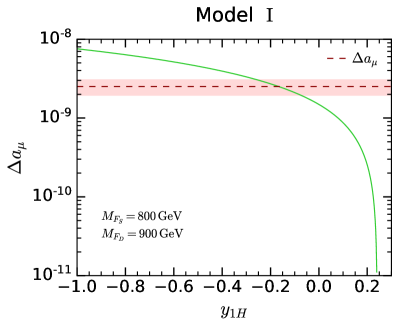
In this section we compute the DM interaction cross sections in Model I. In Fig. 1(a), we show $\Delta a_{\mu}$ as a function of the DM mass $M_{\chi_{1}}$ for $y_{1H}=0.2$ and $-0.2$ in the magenta and cyan solid lines, respectively. The other parameters are fixed to be $y_{2H}=0.3$, $y_{1}=y_{2}=\lambda_{L}=\lambda_{L}^{\prime}=0.5$, $M_{F_{D}}/M_{F_{S}}=1.1$, and $M_{\tilde{L}}/M_{F_{S}}=1.2$. With this parameter choice, we have a singlet-like DM candidate since $M_{F_{S}}<M_{F_{D}}$. The horizontal dashed line indicates the measured value of $\Delta a_{\mu}$ in Eq. (1), with its error indicated by the red band. We see that for $y_{1H}=-0.2$ this model can explain the observed discrepancy in the muon $g-2$ if the DM mass is $\simeq 800$ GeV. It is also shown in Ref. [49] that the thermal relic abundance of $\chi_{1}$ can coincide with the observed DM density with this size of DM mass. Since the new particles in this model are not charged under SU(3)_C, they safely evade the current LHC limits for their masses $\gtrsim 400$ GeV [167]. For the case where $y_{1H}=0.2$, the predicted values of $\Delta a_{\mu}$ are always below the experimental value. To examine the dependence on $y_{1H}$, in Fig. 1(b), we plot $\Delta a_{\mu}$ as a function of $y_{1H}$. For this plot we have fixed the parameters to $M_{F_{S}}=800~{}\mathrm{GeV}$, $M_{F_{D}}=900~{}\mathrm{GeV}$, $M_{\tilde{L}}=1000~{}\mathrm{GeV}$, $y_{1}=y_{2}=\lambda_{L}=\lambda_{L}^{\prime}=0.5$, and $y_{2H}=0.3$. This figure shows that $\Delta a_{\mu}$ decreases as $y_{1H}$ increases, and becomes negative for $y_{1H}\gtrsim 0.25$.

(a) DM mass dependence

(b) $y_{1H}$ dependence

Figure 2: The DM-nucleon SI scattering cross sections as functions of (a) the DM mass $M_{\chi_{1}}$ and (b) $y_{1H}$. The rest of the parameters are fixed as per in Fig. 1. The red shaded area is excluded by the PandaX4T experiment [168] and the yellow shaded region corresponds to the neutrino floor [169].

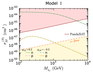
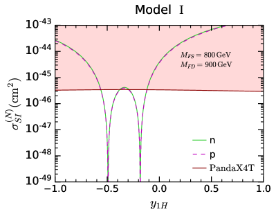
Fig. 2 shows the DM-nucleon SI scattering cross sections as functions of the DM mass $M_{\chi_{1}}$ (Fig. 2(a)) and $y_{1H}$ (Fig. 2(b)). The rest of the parameters are fixed as per in Fig. 1. The red shaded area is excluded by the PandaX4T experiment [168] and the yellow shaded region is out of reach of the present detection strategy due to the neutrino background—the so-called neutrino floor [169]. From these plots, we see that for $y_{1H}=+0.2$, the SI scattering cross section is too large to evade the current experimental limit for $M_{\chi_{1}}\simeq 1~{}\rm TeV$. For $y_{1H}=-0.2$, on the other hand, the SI cross section is much smaller than the current limit, almost on the border of the neutrino floor for $M_{\chi_{1}}\simeq 1\,\rm TeV$. This indicates that it is difficult to test this case in the next-generation DM direct detection experiments.

(a) DM mass dependence

(b) $y_{1H}$ dependence

Figure 3: The DM-nucleon SD scattering cross sections as functions of (a) the DM mass $M_{\chi_{1}}$ and (b) $y_{1H}$. The rest of the parameters are fixed as per in Fig. 1. The blue shaded area is excluded by the XENON1T experiment [170]. The horizontal red band represents the threshold cross section for neutron obtained in Refs. [126, 128], $\sigma_{\mathrm{th}}\simeq[1.7\times 10^{-45},1.4\times 10^{-44}]\,~{}\mathrm{cm}^{2}$.

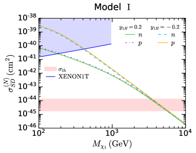
In Fig. 3, the DM-nucleon SD scattering cross sections are shown as functions of the DM mass $M_{\chi_{1}}$ (Fig. 3(a)) and $y_{1H}$ (Fig. 3(b)) with the same parameter choice as in Fig. 1. The blue shaded region is excluded by XENON1T [170] for neutron. We also show the threshold cross section for DM interactions with neutron obtained in Refs. [126, 128], $\sigma_{\mathrm{th}}\simeq[1.7\times 10^{-45},1.4\times 10^{-44}]\,~{}\mathrm{cm}^{2}$, in the horizontal red band. As seen from these plots, the SD scattering cross sections are predicted to be smaller than the XENON1T limit [170] in the parameter regions where the muon $g-2$ discrepancy can be explained. These cross sections are much larger than the threshold cross section $\sigma_{\mathrm{th}}$, and therefore the singlet-like DM candidate in Model I is efficiently captured by NSs.

(a) DM mass dependence

(b) $y_{1H}$ dependence

Figure 4: The DM-muon scattering cross sections as functions of (a) the DM mass $M_{\chi_{1}}$ and (b) $y_{1H}$. The rest of the parameters are fixed as per in Fig. 1. $E_{\mu}$ is varied in the range $[m_{\mu},m_{\mu}/\sqrt{B(R_{\mathrm{NS}})}]$ for $M_{\mathrm{NS}}=1.5~{}M_{\odot}$ and $R_{\mathrm{NS}}=12.593$ km and the resultant change in the cross section is indicated by the band. The horizontal red dashed line shows the threshold cross section for muon, $\sigma_{\mathrm{th}}\simeq 8\times 10^{-44}~{}\mathrm{cm}^{2}$ [127].

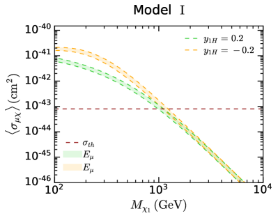
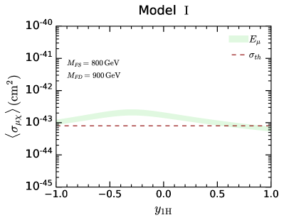
We also compute the DM-muon scattering cross sections adopting the same parameters as in Fig. 1. In this work, we fix the NS mass and radius to be $M_{\mathrm{NS}}=1.5~{}M_{\odot}$ and $R_{\mathrm{NS}}=12.593$ km, respectively, which give $B(R_{\mathrm{NS}})=0.648$ in Eq. (31). The DM-muon scattering cross section is shown in Fig. 4. As we noted in Sec. 5.3, we vary $E_{\mu}$ in the range $[m_{\mu},m_{\mu}/\sqrt{B(R_{\mathrm{NS}})}]$, and the resultant change in the cross section is indicated by the band. We find that the cross section is larger for larger $E_{\mu}$. The horizontal red dashed line shows the threshold cross section for muon, $\sigma_{\mathrm{th}}\simeq 8\times 10^{-44}~{}\mathrm{cm}^{2}$ [127]. We see that the DM-muon scattering cross section also exceeds the threshold cross section in the parameter range motivated by the muon $g-2$ anomaly. Finally, we see in Fig. 4(b) that the DM-muon scattering cross section rarely depends on the coupling $y_{1H}$, in contrast to the DM-nucleon scattering.

6.2 Model I (doublet-like)

(a) DM mass dependence

(b) $y_{1H}$ dependence

Figure 5: $\Delta a_{\mu}$ as a function of (a) the DM mass $M_{\chi_{1}}$ for $y_{1H}=\pm 0.2$, $M_{F_{S}}/M_{F_{D}}=1.1$, and $M_{\tilde{L}}/M_{F_{D}}=1.2$; (b) $y_{1H}$ for $M_{F_{D}}=800~{}\mathrm{GeV}$, $M_{F_{S}}=900~{}\mathrm{GeV}$, and $M_{\tilde{L}}=1000\,\rm GeV$. The rest of the parameters are set to be $y_{1}=y_{2}=\lambda_{L}=\lambda_{L}^{\prime}=0.5$ and $y_{2H}=0.3$. The horizontal dashed line indicates the measured value of $\Delta a_{\mu}$, with its error indicated by the red band.

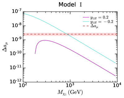
Next, we consider the case where $M_{F_{D}}<M_{F_{S}}$, i.e., the DM is doublet-like. In Fig. 5(a), we show $\Delta a_{\mu}$ as a function of the DM mass $M_{\chi_{1}}$ for $y_{1H}=0.2$ and $-0.2$ in the magenta and cyan solid lines, respectively, with $M_{F_{S}}/M_{F_{D}}=1.1$ and $M_{\tilde{L}}/M_{F_{D}}=1.2$. In Fig. 5(b), we plot $\Delta a_{\mu}$ as a function of $y_{1H}$ for $M_{F_{D}}=800~{}\mathrm{GeV}$, $M_{F_{S}}=900~{}\mathrm{GeV}$, and $M_{\tilde{L}}=1000~{}\mathrm{GeV}$. The rest of the parameters in these figures are fixed to be $y_{1}=y_{2}=\lambda_{L}=\lambda_{L}^{\prime}=0.5$ and $y_{2H}=0.3$. The horizontal dashed line indicates the measured value of $\Delta a_{\mu}$ in Eq. (1), with its error indicated by the red band. The behavior of $\Delta a_{\mu}$ is similar to that in Fig. 1 and a negative value of $y_{1H}$ and $\sim 1\,\rm TeV$ DM mass can explain the observed discrepancy in the muon $g-2$.

(a) DM mass dependence

(b) $y_{1H}$ dependence

Figure 6: The DM-nucleon SI scattering cross sections as functions of (a) the DM mass $M_{\chi_{1}}$ and (b) $y_{1H}$. The rest of the parameters are fixed as in Fig. 5. The red shaded area is excluded by the PandaX4T experiment [168] and the yellow shaded region corresponds to the neutrino floor [169].

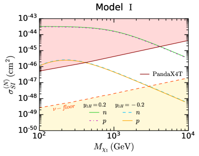
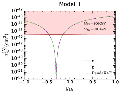
The DM-nucleon SI scattering cross sections are shown as functions of the DM mass $M_{\chi_{1}}$ and $y_{1H}$ in Fig. 6(a) and Fig. 6(b), respectively. The rest of the parameters are fixed as in Fig. 5. The red shaded region represents the PandaX4T bound [168] and the yellow shaded region corresponds to the neutrino floor [169]. We see that the behavior of the SI scattering cross sections for $y_{1H}=+0.2$ is similar to that in Fig. 2(a). For $y_{1H}=-0.2$, on the other hand, the SI cross sections are predicted to be larger than those for the singlet-like case, and within reach of future DM direct detection experiments for the DM mass $\sim 1\,\rm TeV$.

(a) DM mass dependence

(b) $y_{1H}$ dependence

Figure 7: The DM-nucleon SD scattering cross sections as functions of (a) the DM mass $M_{\chi_{1}}$ and (b) $y_{1H}$. The rest of the parameters are fixed as in Fig. 5. The blue shaded area is excluded by the XENON1T experiment [170]. The horizontal red band represents the threshold cross section for neutron obtained in Refs. [126, 128].

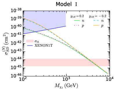
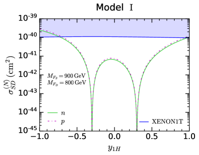
In Fig. 7, the DM-nucleon SD scattering cross sections are shown as functions of the DM mass $M_{\chi_{1}}$ (Fig. 7(a)) and $y_{1H}$ (Fig. 7(b)) with the same parameter choice as in Fig. 5. The blue shaded region is excluded by XENON1T [170] for neutron and the horizontal red band represents the threshold cross section for neutron obtained in Refs. [126, 128]. We see that the behavior of the SD cross sections is similar to that in Fig. 7 and the XENON1T limit is evaded in the $g-2$ favored parameter regions. The DM is efficiently captured by NSs for $M_{\chi_{1}}\lesssim 3\,\rm TeV$.

(a) DM mass dependence

(b) $y_{1H}$ dependence

Figure 8: The DM-muon scattering cross sections as functions of (a) the DM mass $M_{\chi_{1}}$ and (b) $y_{1H}$. The rest of the parameters are fixed as per in Fig. 5. $E_{\mu}$ is varied in the range $[m_{\mu},m_{\mu}/\sqrt{B(R_{\mathrm{NS}})}]$ for $M_{\mathrm{NS}}=1.5~{}M_{\odot}$ and $R_{\mathrm{NS}}=12.593$ km and the resultant change in the cross section is indicated by the band. The horizontal red dashed line shows the threshold cross section for muon, $\sigma_{\mathrm{th}}\simeq 8\times 10^{-44}~{}\mathrm{cm}^{2}$ [127].

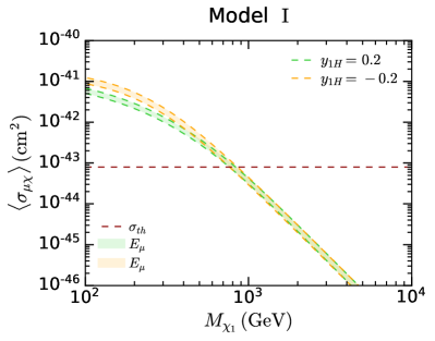
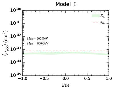
Figure 8 shows the DM-muon scattering cross sections, where the parameters are fixed as in Fig. 5. We again vary $E_{\mu}$ in the range $[m_{\mu},m_{\mu}/\sqrt{B(R_{\mathrm{NS}})}]$, for the same NS configuration, which is indicated by the band. The horizontal red dashed line shows the threshold cross section for muon, $\sigma_{\mathrm{th}}\simeq 8\times 10^{-44}~{}\mathrm{cm}^{2}$ [127]. The DM-muon scattering cross section is predicted to be smaller than that in the singlet-like DM case and nearly equal to the threshold cross section in the $g-2$ favored parameter range.

6.3 Model II

(a) $\Delta a_{\mu}$

(b) DM-muon scattering cross section

Figure 9: (a) $\Delta a_{\mu}$ as a function of the DM mass $M_{F_{S}}$. The horizontal dashed line indicates the measured value of $\Delta a_{\mu}$, with its error indicated by the red band. (b) DM-muon scattering cross section as a function of the DM mass $M_{F_{S}}$. $E_{\mu}$ is varied in the range $[m_{\mu},m_{\mu}/\sqrt{B(R_{\mathrm{NS}})}]$ for $M_{\mathrm{NS}}=1.5~{}M_{\odot}$ and $R_{\mathrm{NS}}=12.593$ km and the resultant change in the cross section is indicated by the band. The horizontal red dashed line shows the threshold cross section for muon, $\sigma_{\mathrm{th}}\simeq 8\times 10^{-44}~{}\mathrm{cm}^{2}$ [127]. We set $M_{\tilde{\bar{e}}}/M_{F_{S}}=1.1$, $M_{\tilde{L}}/M_{F_{S}}=1.2$, $a_{H}=M_{F_{S}}/2$, and $y_{1}=y_{2}=\lambda_{L}=\lambda_{\bar{e}}=\lambda_{L}^{\prime}=0.5$.

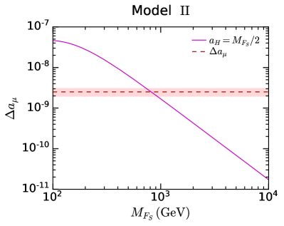
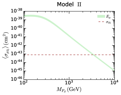
Finally, we study Model II. As discussed in Sec. 4 and Sec. 5.2, the DM-nucleon scattering is induced at the loop level in this case. As a result, the SI scattering cross section is too small to be probed in future DM direct searches and the SD scattering cross section lies below the threshold cross section in the parameter regions of our interest. We thus consider only $\Delta a_{\mu}$ and the DM-muon scattering cross section for Model II, which are shown as functions of the DM mass in Fig. 9(a) and Fig. 9(b), respectively. We set $M_{\tilde{\bar{e}}}/M_{F_{S}}=1.1$, $M_{\tilde{L}}/M_{F_{S}}=1.2$, $a_{H}=M_{F_{S}}/2$, and $y_{1}=y_{2}=\lambda_{L}=\lambda_{\bar{e}}=\lambda_{L}^{\prime}=0.5$ in both of the plots. The observed deviation in the muon $g-2$ can be explained for the DM mass $\simeq 800~{}\rm GeV$ with this parameter choice. As shown in Ref. [50], the observed DM density can be explained with this size of the DM mass, without conflicting with the LHC limits. For this DM mass, the DM-muon scattering cross section is much larger than the threshold cross section, as illustrated in Fig. 9(b). Consequently, in Model II, the DM efficiently accumulates in NSs through the DM-muon scattering, not via the DM-nucleon scattering as in Model I. Given that it is very difficult to probe this DM candidate in DM direct detection experiments and the LHC experiments, the DM search using the NS temperature observation plays an important role in testing this scenario in the future.

7 Conclusion and discussion

We have studied two representative DM models, Model I and II, where WIMP DM particles have renormalizable couplings to muons. In both of these models, the experimental value of the muon $g-2$ can be explained with a DM mass of $\sim 1~{}\mathrm{TeV}$. Such a heavy DM particle, as well as heavier colorless states in the models, is beyond the reach of the LHC experiments. In Model I, the SI DM-nucleon scattering cross section is predicted to be generically rather large, but in the muon $g-2$ favored parameter regions, it is found to be much smaller than the current experimental limit and may be probed in future DM direct detection experiments. The SD DM-nucleon scattering cross section is larger than the threshold cross section. On the other hand, in Model II, both the SI and SD DM-nucleon scattering cross sections are highly suppressed, and it is hard to probe this model in DM direct detection experiments. However, we find that even in this case the DM particles efficiently accumulate in NSs since the DM-muon scattering cross section is sufficiently larger than the threshold cross section. As a result, in both of these models, the DM capture in NSs is effective and the DM heating operates maximally. Our study thus indicates that the temperature observation of old NSs provides a promising way of testing the WIMP DM models for the muon $g-2$ discrepancy.

Although we have considered only simple setups in this paper, we expect that the same conclusion holds in a variety of more realistic WIMP DM models. For example, in the framework of SUSY, the bino-slepton system provides a setup similar to Model II. As demonstrated in Ref. [60], this system can explain the muon $g-2$ discrepancy and the observed DM density with a $\sim 100$ GeV bino DM and sleptons. The DM-muon coupling in this case is given by the hypercharge gauge coupling, $g^{\prime}\simeq 0.36$, which is smaller than $y_{1}=y_{2}=0.5$ taken in Fig. 9. However, the bino DM mass is smaller than the favored value of $M_{F_{S}}$ in Fig. 9 by a factor of $\sim 8$, and therefore the DM-muon scattering cross section is much larger than that in Model II. This simple estimate shows that we can test the SUSY explanations of the muon $g-2$ discrepancy by means of the search of the DM heating in NSs. Such a model-specific study is beyond the scope of this paper, and we defer it to another occasion.

Appendix

Appendix A Interactions in the mass eigenbasis

In this Appendix, we summarize the interaction terms expressed in terms of mass eigenfields.

A.1 Model I

A.1.1 Gauge interactions

The interactions of the new particles with a photon are

$$\mathcal{L}_{A} =e\overline{\psi^{-}}\gamma^{\mu}\psi^{-}A_{\mu}+e\widetilde{e}^{*}i\overleftrightarrow{\partial^{\mu}}\widetilde{e}A_{\mu}~{},$$ (A.1)

where $e>0$ is the electric charge of positron, $A\overleftrightarrow{\partial^{\mu}}B\equiv A(\partial^{\mu}B)-(\partial^{\mu}A)B$, and we introduce the four-component Dirac notation,

$$\psi^{-}\equiv\begin{pmatrix}\xi_{D^{-}}\\ \eta^{\dagger}_{D^{+}}\end{pmatrix}~{}.$$ (A.2)

For the couplings with a $Z$ boson, only the dark matter-$Z$ coupling is relevant for our discussion:

$$\mathcal{L}_{{\mathrm{DM-}}Z}=-\frac{g_{Z}}{4}\left[\left|\left(V_{\chi}\right)_{21}\right|^{2}-\left|\left(V_{\chi}\right)_{31}\right|^{2}\right]\overline{\psi^{0}_{1}}\gamma^{\mu}\gamma_{5}\psi^{0}_{1}Z_{\mu}~{},$$ (A.3)

where $g_{Z}\equiv\sqrt{g^{\prime 2}+g^{2}}$ with $g^{\prime}$ and $g$ the U(1)_Y and SU(2)_L gauge coupling constants, respectively, and $\psi^{0}_{i}$ $(i=1,2,3)$ are four-component Majorana fermions defined by

$$\psi^{0}_{i}\equiv\begin{pmatrix}\chi_{i}\\ \chi_{i}^{\dagger}\end{pmatrix}~{}.$$ (A.4)

A.1.2 Yukawa interactions

In the unitary gauge

$$H=\frac{1}{\sqrt{2}}\begin{pmatrix}0\\ v+h\end{pmatrix}~{},$$ (A.5)

the Yukawa interactions are written as

$$\mathcal{L}_{\mathrm{Yukawa}}= -\frac{h}{\sqrt{2}}\overline{\psi^{0}_{i}}\left[\left(C_{\chi hL}\right)_{ij}P_{L}+\left(C_{\chi hR}\right)_{ij}P_{R}\right]\psi_{j}^{0}$$

$$-\left\{\overline{\psi^{0}_{i}}\left[y_{1}\left(V_{\chi}\right)_{1i}P_{L}+y_{2}^{*}\left(V_{\chi}\right)^{*}_{2i}P_{R}\right]\mu\,\widetilde{e}^{*}+\mathrm{h.c.}\right\}$$

$$-\left[y_{1}\left(V_{\chi}\right)_{1i}\overline{\psi^{0}_{i}}P_{L}\nu\widetilde{\nu}^{*}-y_{2}\bar{\mu}P_{L}\psi^{-}\widetilde{\nu}+\mathrm{h.c.}\right]~{},$$ (A.6)

with $P_{L/R}\equiv(1\mp\gamma_{5})/2$ and

$$\left(C_{\chi hL}\right)_{ij} \equiv\left(V_{\chi}\right)_{1i}\left[y_{1H}\left(V_{\chi}\right)_{2j}+y_{2H}\left(V_{\chi}\right)_{3j}\right]~{},\qquad\left(C_{\chi hR}\right)_{ij}\equiv\left(C_{\chi hL}\right)_{ji}^{*}~{}.$$ (A.7)

A.2 Model II

A.2.1 Gauge interactions

For interactions with a photon, we have

$$\mathcal{L}_{A} =e\sum_{i=1,2}\widetilde{e}_{i}^{*}i\overleftrightarrow{\partial^{\mu}}\widetilde{e}_{i}A_{\mu}~{},$$ (A.8)

while for those with a $Z$-boson,

$$\mathcal{L}_{Z} =\frac{g_{Z}}{2}\widetilde{\nu}^{*}i\overleftrightarrow{\partial^{\mu}}\widetilde{\nu}Z_{\mu}+g_{Z}\left[-\frac{1}{2}\left(U_{e}^{*}\right)_{1i}\left(U_{e}\right)_{1j}+\sin^{2}\theta_{W}\delta_{ij}\right]\widetilde{e}_{i}^{*}i\overleftrightarrow{\partial^{\mu}}\widetilde{e}_{j}Z_{\mu}$$ (A.9)

where $\theta_{W}$ is the weak mixing angle.

A.2.2 Yukawa interactions

The Yukawa interactions in Model II are

$$\mathcal{L}_{\mathrm{Yukawa}}= -\left\{\overline{\psi^{0}}\left[y_{1}\left(U_{e}\right)_{1i}^{*}P_{L}+y_{2}^{*}\left(U_{e}\right)^{*}_{2i}P_{R}\right]\mu\,\widetilde{e}_{i}^{*}+\mathrm{h.c.}\right\}$$

$$-\left[y_{1}\overline{\psi^{0}}P_{L}\nu\widetilde{\nu}^{*}+\mathrm{h.c.}\right]~{},$$ (A.10)

where $\psi^{0}$ is a four-component Majorana fermion defined by

$$\psi^{0}\equiv\begin{pmatrix}\chi_{S}\\ \chi_{S}^{\dagger}\end{pmatrix}~{}.$$ (A.11)

A.2.3 Scalar trilinear interaction

In the unitary gauge (A.5), the scalar trilinear coupling is obtained from Eq. (15) and Eq. (16) as

$$\mathcal{L}_{\mathrm{tri}} =-\left(C_{h\widetilde{e}}\right)_{ij}h\widetilde{e}_{i}^{*}\widetilde{e}_{j}-v(\lambda_{L}-\lambda_{L}^{\prime})h\left|\widetilde{\nu}\right|^{2}~{},$$ (A.12)

where

$$\left(C_{h\widetilde{e}}\right)_{ij} \equiv\frac{1}{\sqrt{2}}\left[a_{H}\left(U_{e}\right)^{*}_{2i}\left(U_{e}\right)_{1j}+a_{H}^{*}\left(U_{e}\right)^{*}_{1i}\left(U_{e}\right)_{2j}\right]$$

$$+v\left[(\lambda_{L}+\lambda_{L}^{\prime})\left(U_{e}\right)_{1i}^{*}\left(U_{e}\right)_{1j}+\lambda_{\bar{e}}\left(U_{e}\right)_{2i}^{*}\left(U_{e}\right)_{2j}\right]~{}.$$ (A.13)

Appendix B Amplitudes for the DM–$\mu$ scattering

In this section, we show the expressions for the scattering amplitudes in Model I and II in Sec. B.1 and Sec. B.2, respectively. We expand the invariant scattering amplitude as in Eq. (42):

$$\frac{1}{4}\sum_{\mathrm{spins}}|\mathcal{A}|^{2}\simeq\alpha_{0}+\alpha_{1}\,(-t)~{},$$ (B.1)

and give the expressions of $\alpha_{0}$ and $\alpha_{1}$. We take account of the hierarchy, $\bar{s}\simeq M_{\mathrm{DM}}^{2}\gg\bar{s}-M_{\mathrm{DM}}^{2}\simeq 2E_{\chi}E_{\mu}\gg|t|,E_{\mu}^{2}$, and keep only the leading order terms, which turn out to be $\mathcal{O}(E_{\mu}^{2}/E_{\chi}^{2})$.

B.1 Model I

$$\alpha_{0}=\frac{1}{2\left(M_{\tilde{e}}^{2}-M_{\chi_{1}}^{2}\right)^{2}} \Bigl{[}\left(s-M_{\chi_{1}}^{2}\right)^{2}\left\{\left|y_{1}(V_{\chi})_{11}\right|^{2}+\left|y_{2}(V_{\chi})_{21}\right|^{2}\right\}^{2}$$

$$+16m_{\mu}^{2}M_{\chi_{1}}^{2}\left\{\mathrm{Re}\left[y_{1}y_{2}(V_{\chi})_{11}(V_{\chi})_{21}\right]\right\}^{2}$$

$$+2m_{\mu}^{2}M_{\chi_{1}}^{2}\left\{\left|y_{1}(V_{\chi})_{11}\right|^{4}+\left|y_{2}(V_{\chi})_{21}\right|^{4}\right\}$$

$$-2\left|y_{1}(V_{\chi})_{11}\right|^{2}\left|y_{2}(V_{\chi})_{21}\right|^{2}\left\{(s-M_{\chi_{1}}^{2})^{2}-4m_{\mu}^{2}M_{\chi_{1}}^{2}\right\}$$

$$-4m_{\mu}^{2}M_{\chi_{1}}^{2}\mathrm{Re}\left\{y_{1}^{2}y_{2}^{2}(V_{\chi})_{11}^{2}(V_{\chi})_{21}^{2}\right\}\Bigr{]}~{}.$$ (B.2)

$$\alpha_{1} =\frac{M_{\chi_{1}}^{2}\left\{\left|y_{1}(V_{\chi})_{11}\right|^{2}+\left|y_{2}(V_{\chi})_{21}\right|^{2}\right\}^{2}}{2\left(M_{\tilde{e}}^{2}-M_{\chi_{1}}^{2}\right)^{2}}~{}.$$ (B.3)

B.2 Model II

$$\alpha_{0}=\sum_{i=1,2}\frac{1}{(M_{F_{S}}^{2}-M_{e_{i}}^{2})(M_{F_{S}}^{2}-M_{e_{j}}^{2})} \times$$

$$\times\Bigg{[}\frac{1}{2}(M_{F_{S}}^{2}-s)^{2} \big{[}y_{1}^{4}|(U_{e})_{1i}|^{2}|(U_{e})_{1j}|^{2}+y_{2}^{4}|(U_{e})_{2i}|^{2}|(U_{e})_{2j}|^{2}\big{]}$$

$$+m_{\mu}^{2}M_{F_{S}}^{2}\Big{[}3 y_{1}^{2}y_{2}^{2}|(U_{e})_{1i}|^{2}|(U_{e})_{2j}|^{2}+3y_{1}^{2}y_{2}^{2}|(U_{e})_{1j}|^{2}|(U_{e})_{2i}|^{2}$$

$$+y_{1}^{4}|(U_{e})_{1i}|^{2}|(U_{e})_{1j}|^{2}+y_{2}^{4}|(U_{e})_{2i}|^{2}|(U_{e})_{2j}|^{2}$$

$$+2y_{1}^{2}y_{2}^{2}\mathrm{Re}[(U_{e})_{1i}(U_{e}^{\ast})_{1j}(U_{e}^{\ast})_{2i}(U_{e})_{2j}]$$

$$+2y_{1}^{2}y_{2}^{2}\mathrm{Re}[(U_{e})_{1i}(U_{e})_{1j}(U_{e}^{\ast})_{2i}(U_{e}^{\ast})_{2j}]\Big{]}\Bigg{]}$$ (B.4)

$$\alpha_{1}= \sum_{i=1,2}\frac{M_{F_{S}}^{2}}{2(M_{F_{S}}^{2}-M_{e_{i}}^{2})(M_{F_{S}}^{2}-M_{e_{j}}^{2})}\times$$

$$\times\Bigg{[}y_{1}^{4}|(U_{e})_{1i}|^{2}|(U_{e})_{1j}|^{2}+y_{2}^{4}|(U_{e})_{2i}|^{2}|(U_{e})_{2j}|^{2}+2\mathrm{Re}[(U_{e})_{1i}(U_{e}^{\ast})_{1j}(U_{e}^{\ast})_{2i}(U_{e})_{2j}]\Bigg{]}$$ (B.5)

References

- [1] Muon g-2 Collaboration, Measurement of the Positive Muon Anomalous Magnetic Moment to 0.46 ppm, Phys. Rev. Lett. 126 (2021) 141801 [arXiv:2104.03281].
- [2] T. Aoyama et al., The anomalous magnetic moment of the muon in the Standard Model, Phys. Rept. 887 (2020) 1–166 [arXiv:2006.04822].
- [3] M. Davier, A. Hoecker, B. Malaescu, and Z. Zhang, Reevaluation of the hadronic vacuum polarisation contributions to the Standard Model predictions of the muon and using newest hadronic cross-section data, Eur. Phys. J. C77 (2017) 827 [arXiv:1706.09436].
- [4] A. Keshavarzi, D. Nomura, and T. Teubner, Muon and : a new data-based analysis, Phys. Rev. D97 (2018) 114025 [arXiv:1802.02995].
- [5] G. Colangelo, M. Hoferichter, and P. Stoffer, Two-pion contribution to hadronic vacuum polarization, JHEP 02 (2019) 006 [arXiv:1810.00007].
- [6] M. Hoferichter, B.-L. Hoid, and B. Kubis, Three-pion contribution to hadronic vacuum polarization, JHEP 08 (2019) 137 [arXiv:1907.01556].
- [7] M. Davier, A. Hoecker, B. Malaescu, and Z. Zhang, A new evaluation of the hadronic vacuum polarisation contributions to the muon anomalous magnetic moment and to , Eur. Phys. J. C80 (2020) 241 [arXiv:1908.00921]. [Erratum: Eur. Phys. J. C80, 410 (2020)].
- [8] A. Keshavarzi, D. Nomura, and T. Teubner, The of charged leptons, and the hyperfine splitting of muonium, Phys. Rev. D101 (2020) 014029 [arXiv:1911.00367].
- [9] A. Kurz, T. Liu, P. Marquard, and M. Steinhauser, Hadronic contribution to the muon anomalous magnetic moment to next-to-next-to-leading order, Phys. Lett. B734 (2014) 144–147 [arXiv:1403.6400].
- [10] Fermilab Lattice, LATTICE-HPQCD, MILC Collaboration, Strong-Isospin-Breaking Correction to the Muon Anomalous Magnetic Moment from Lattice QCD at the Physical Point, Phys. Rev. Lett. 120 (2018) 152001 [arXiv:1710.11212].
- [11] Budapest-Marseille-Wuppertal Collaboration, Hadronic vacuum polarization contribution to the anomalous magnetic moments of leptons from first principles, Phys. Rev. Lett. 121 (2018) 022002 [arXiv:1711.04980].
- [12] RBC, UKQCD Collaboration, Calculation of the hadronic vacuum polarization contribution to the muon anomalous magnetic moment, Phys. Rev. Lett. 121 (2018) 022003 [arXiv:1801.07224].
- [13] ETM Collaboration, Electromagnetic and strong isospin-breaking corrections to the muon from Lattice QCD+QED, Phys. Rev. D99 (2019) 114502 [arXiv:1901.10462].
- [14] E. Shintani and Y. Kuramashi, Study of systematic uncertainties in hadronic vacuum polarization contribution to muon with 2+1 flavor lattice QCD, Phys. Rev. D100 (2019) 034517 [arXiv:1902.00885].
- [15] Fermilab Lattice, LATTICE-HPQCD, MILC Collaboration, Hadronic-vacuum-polarization contribution to the muon’s anomalous magnetic moment from four-flavor lattice QCD, Phys. Rev. D101 (2020) 034512 [arXiv:1902.04223].
- [16] A. Gérardin, et al., The leading hadronic contribution to from lattice QCD with flavours of O() improved Wilson quarks, Phys. Rev. D100 (2019) 014510 [arXiv:1904.03120].
- [17] C. Aubin, et al., Light quark vacuum polarization at the physical point and contribution to the muon , Phys. Rev. D101 (2020) 014503 [arXiv:1905.09307].
- [18] D. Giusti and S. Simula, Lepton anomalous magnetic moments in Lattice QCD+QED, PoS LATTICE2019 (2019) 104 [arXiv:1910.03874].
- [19] P. Masjuan and P. Sánchez-Puertas, Pseudoscalar-pole contribution to the : a rational approach, Phys. Rev. D95 (2017) 054026 [arXiv:1701.05829].
- [20] G. Colangelo, M. Hoferichter, M. Procura, and P. Stoffer, Dispersion relation for hadronic light-by-light scattering: two-pion contributions, JHEP 04 (2017) 161 [arXiv:1702.07347].
- [21] M. Hoferichter, B.-L. Hoid, B. Kubis, S. Leupold, and S. P. Schneider, Dispersion relation for hadronic light-by-light scattering: pion pole, JHEP 10 (2018) 141 [arXiv:1808.04823].
- [22] A. Gérardin, H. B. Meyer, and A. Nyffeler, Lattice calculation of the pion transition form factor with Wilson quarks, Phys. Rev. D100 (2019) 034520 [arXiv:1903.09471].
- [23] J. Bijnens, N. Hermansson-Truedsson, and A. Rodríguez-Sánchez, Short-distance constraints for the HLbL contribution to the muon anomalous magnetic moment, Phys. Lett. B798 (2019) 134994 [arXiv:1908.03331].
- [24] G. Colangelo, F. Hagelstein, M. Hoferichter, L. Laub, and P. Stoffer, Longitudinal short-distance constraints for the hadronic light-by-light contribution to with large- Regge models, JHEP 03 (2020) 101 [arXiv:1910.13432].
- [25] V. Pauk and M. Vanderhaeghen, Single meson contributions to the muon‘s anomalous magnetic moment, Eur. Phys. J. C74 (2014) 3008 [arXiv:1401.0832].
- [26] I. Danilkin and M. Vanderhaeghen, Light-by-light scattering sum rules in light of new data, Phys. Rev. D95 (2017) 014019 [arXiv:1611.04646].
- [27] F. Jegerlehner, The Anomalous Magnetic Moment of the Muon, Springer Tracts Mod. Phys. 274 (2017) 1–693.
- [28] M. Knecht, S. Narison, A. Rabemananjara, and D. Rabetiarivony, Scalar meson contributions to from hadronic light-by-light scattering, Phys. Lett. B787 (2018) 111–123 [arXiv:1808.03848].
- [29] G. Eichmann, C. S. Fischer, and R. Williams, Kaon-box contribution to the anomalous magnetic moment of the muon, Phys. Rev. D101 (2020) 054015 [arXiv:1910.06795].
- [30] P. Roig and P. Sánchez-Puertas, Axial-vector exchange contribution to the hadronic light-by-light piece of the muon anomalous magnetic moment, Phys. Rev. D101 (2020) 074019 [arXiv:1910.02881].
- [31] G. Colangelo, M. Hoferichter, A. Nyffeler, M. Passera, and P. Stoffer, Remarks on higher-order hadronic corrections to the muon , Phys. Lett. B735 (2014) 90–91 [arXiv:1403.7512].
- [32] T. Blum, et al., The hadronic light-by-light scattering contribution to the muon anomalous magnetic moment from lattice QCD, Phys. Rev. Lett. 124 (2020) 132002 [arXiv:1911.08123].
- [33] T. Aoyama, M. Hayakawa, T. Kinoshita, and M. Nio, Complete Tenth-Order QED Contribution to the Muon , Phys. Rev. Lett. 109 (2012) 111808 [arXiv:1205.5370].
- [34] T. Aoyama, T. Kinoshita, and M. Nio, Theory of the Anomalous Magnetic Moment of the Electron, Atoms 7 (2019) 28.
- [35] A. Czarnecki, W. J. Marciano, and A. Vainshtein, Refinements in electroweak contributions to the muon anomalous magnetic moment, Phys. Rev. D67 (2003) 073006 [hep-ph/0212229]. [Erratum: Phys. Rev. D73, 119901 (2006)].
- [36] C. Gnendiger, D. Stöckinger, and H. Stöckinger-Kim, The electroweak contributions to after the Higgs boson mass measurement, Phys. Rev. D88 (2013) 053005 [arXiv:1306.5546].
- [37] K. Melnikov and A. Vainshtein, Hadronic light-by-light scattering contribution to the muon anomalous magnetic moment revisited, Phys. Rev. D70 (2004) 113006 [hep-ph/0312226].
- [38] Muon g-2 Collaboration, Final Report of the Muon E821 Anomalous Magnetic Moment Measurement at BNL, Phys. Rev. D 73 (2006) 072003 [hep-ex/0602035].
- [39] S. Borsanyi et al., Leading hadronic contribution to the muon magnetic moment from lattice QCD, Nature 593 (2021) 51–55 [arXiv:2002.12347].
- [40] C. Lehner and A. S. Meyer, Consistency of hadronic vacuum polarization between lattice QCD and the R-ratio, Phys. Rev. D 101 (2020) 074515 [arXiv:2003.04177].
- [41] A. Crivellin, M. Hoferichter, C. A. Manzari, and M. Montull, Hadronic Vacuum Polarization: versus Global Electroweak Fits, Phys. Rev. Lett. 125 (2020) 091801 [arXiv:2003.04886].
- [42] A. Keshavarzi, W. J. Marciano, M. Passera, and A. Sirlin, Muon and connection, Phys. Rev. D 102 (2020) 033002 [arXiv:2006.12666].
- [43] E. de Rafael, Constraints between and , Phys. Rev. D 102 (2020) 056025 [arXiv:2006.13880].
- [44] B. Malaescu and M. Schott, Impact of correlations between and on the EW fit, Eur. Phys. J. C 81 (2021) 46 [arXiv:2008.08107].
- [45] L. Di Luzio, A. Masiero, P. Paradisi, and M. Passera, New physics behind the new muon -2 puzzle?, arXiv:2112.08312 (2021).
- [46] G. Colangelo, M. Hoferichter, and P. Stoffer, Constraints on the two-pion contribution to hadronic vacuum polarization, Phys. Lett. B 814 (2021) 136073 [arXiv:2010.07943].
- [47] S. Kanemitsu and K. Tobe, New physics for muon anomalous magnetic moment and its electroweak precision analysis, Phys. Rev. D 86 (2012) 095025 [arXiv:1207.1313].
- [48] K. Kowalska and E. M. Sessolo, Expectations for the muon g-2 in simplified models with dark matter, JHEP 09 (2017) 112 [arXiv:1707.00753].
- [49] L. Calibbi, R. Ziegler, and J. Zupan, Minimal models for dark matter and the muon g2 anomaly, JHEP 07 (2018) 046 [arXiv:1804.00009].
- [50] J. Kawamura, S. Okawa, and Y. Omura, Current status and muon explanation of lepton portal dark matter, JHEP 08 (2020) 042 [arXiv:2002.12534].
- [51] S.-I. Horigome, T. Katayose, S. Matsumoto, and I. Saha, Leptophilic fermion WIMP: Role of future lepton colliders, Phys. Rev. D 104 (2021) 055001 [arXiv:2102.08645].
- [52] G. Arcadi, L. Calibbi, M. Fedele, and F. Mescia, Muon and -anomalies from Dark Matter, Phys. Rev. Lett. 127 (2021) 061802 [arXiv:2104.03228].
- [53] Y. Bai and J. Berger, Muon in Lepton Portal Dark Matter, arXiv:2104.03301 (2021).
- [54] P. Athron, et al., New physics explanations of in light of the FNAL muon measurement, JHEP 09 (2021) 080 [arXiv:2104.03691].
- [55] J. T. Acuña, P. Stengel, and P. Ullio, A Minimal Dark Matter Model for Muon g-2 with Scalar Lepton Partners up to the TeV Scale, arXiv:2112.08992 (2021).
- [56] T. Ghosh, C. Kelso, J. Kumar, P. Sandick, and P. Stengel in 2022 Snowmass Summer Study. 2022. arXiv:2203.08107.
- [57] J. L. Lopez, D. V. Nanopoulos, and X. Wang, Large (g-2)-mu in SU(5) x U(1) supergravity models, Phys. Rev. D 49 (1994) 366–372 [hep-ph/9308336].
- [58] U. Chattopadhyay and P. Nath, Probing supergravity grand unification in the Brookhaven g-2 experiment, Phys. Rev. D 53 (1996) 1648–1657 [hep-ph/9507386].
- [59] T. Moroi, The Muon anomalous magnetic dipole moment in the minimal supersymmetric standard model, Phys. Rev. D 53 (1996) 6565–6575 [hep-ph/9512396]. [Erratum: Phys.Rev.D 56, 4424 (1997)].
- [60] M. Endo, K. Hamaguchi, S. Iwamoto, and T. Kitahara, Supersymmetric interpretation of the muon anomaly, JHEP 07 (2021) 075 [arXiv:2104.03217].
- [61] S. Iwamoto, T. T. Yanagida, and N. Yokozaki, Wino-Higgsino dark matter in MSSM from the anomaly, Phys. Lett. B 823 (2021) 136768 [arXiv:2104.03223].
- [62] Y. Gu, N. Liu, L. Su, and D. Wang, Heavy bino and slepton for muon anomaly, Nucl. Phys. B 969 (2021) 115481 [arXiv:2104.03239].
- [63] W. Yin, Muon anomaly in anomaly mediation, JHEP 06 (2021) 029 [arXiv:2104.03259].
- [64] F. Wang, L. Wu, Y. Xiao, J. M. Yang, and Y. Zhang, GUT-scale constrained SUSY in light of new muon measurement, Nucl. Phys. B 970 (2021) 115486 [arXiv:2104.03262].
- [65] M. Abdughani, et al., A common origin of muon anomaly, Galaxy Center GeV excess and AMS-02 anti-proton excess in the NMSSM, Sci. Bull. 66 (2021) 1545 [arXiv:2104.03274].
- [66] J. Cao, J. Lian, Y. Pan, D. Zhang, and P. Zhu, Improved (g - 2)μ measurement and singlino dark matter in -term extended -NMSSM, JHEP 09 (2021) 175 [arXiv:2104.03284].
- [67] M. Chakraborti, S. Heinemeyer, and I. Saha, The new “MUON G-2” result and supersymmetry, Eur. Phys. J. C 81 (2021) 1114 [arXiv:2104.03287].
- [68] M. Ibe, S. Kobayashi, Y. Nakayama, and S. Shirai, Muon in Gauge Mediation without SUSY CP Problem, arXiv:2104.03289 (2021).
- [69] P. Cox, C. Han, and T. T. Yanagida, Muon g-2 and coannihilating dark matter in the minimal supersymmetric standard model, Phys. Rev. D 104 (2021) 075035 [arXiv:2104.03290].
- [70] S. Heinemeyer, et al., The new result and the SSM, Eur. Phys. J. C 81 (2021) 802 [arXiv:2104.03294].
- [71] S. Baum, M. Carena, N. R. Shah, and C. E. M. Wagner, The tiny (g-2) muon wobble from small- supersymmetry, JHEP 01 (2022) 025 [arXiv:2104.03302].
- [72] H.-B. Zhang, C.-X. Liu, J.-L. Yang, and T.-F. Feng, Muon anomalous magnetic dipole moment in the SSM, arXiv:2104.03489 (2021).
- [73] W. Ahmed, et al., The natural explanation of the muon anomalous magnetic moment via the electroweak supersymmetry from the GmSUGRA in the MSSM, Phys. Lett. B 827 (2022) 136879 [arXiv:2104.03491].
- [74] A. Aboubrahim, M. Klasen, and P. Nath, What the Fermilab muon 2 experiment tells us about discovering supersymmetry at high luminosity and high energy upgrades to the LHC, Phys. Rev. D 104 (2021) 035039 [arXiv:2104.03839].
- [75] M. Chakraborti, L. Roszkowski, and S. Trojanowski, GUT-constrained supersymmetry and dark matter in light of the new determination, JHEP 05 (2021) 252 [arXiv:2104.04458].
- [76] H. Baer, V. Barger, and H. Serce, Anomalous muon magnetic moment, supersymmetry, naturalness, LHC search limits and the landscape, Phys. Lett. B 820 (2021) 136480 [arXiv:2104.07597].
- [77] W. Altmannshofer, S. A. Gadam, S. Gori, and N. Hamer, Explaining (g 2)μ with multi-TeV sleptons, JHEP 07 (2021) 118 [arXiv:2104.08293].
- [78] A. Aboubrahim, P. Nath, and R. M. Syed, Yukawa coupling unification in an SO(10) model consistent with Fermilab (g 2)μ result, JHEP 06 (2021) 002 [arXiv:2104.10114].
- [79] M. Chakraborti, S. Heinemeyer, and I. Saha in International Workshop on Future Linear Colliders. 2021. arXiv:2105.06408.
- [80] M.-D. Zheng and H.-H. Zhang, Studying the anomalies and in -parity violating MSSM framework with the inverse seesaw mechanism, Phys. Rev. D 104 (2021) 115023 [arXiv:2105.06954].
- [81] K. S. Jeong, J. Kawamura, and C. B. Park, Mixed modulus and anomaly mediation in light of the muon g 2 anomaly, JHEP 10 (2021) 064 [arXiv:2106.04238].
- [82] Z. Li, G.-L. Liu, F. Wang, J. M. Yang, and Y. Zhang, Gluino-SUGRA scenarios in light of FNAL muon g – 2 anomaly, JHEP 12 (2021) 219 [arXiv:2106.04466].
- [83] J. S. Kim, D. E. Lopez-Fogliani, A. D. Perez, and R. R. de Austri, The new (g2) and right-handed sneutrino dark matter, Nucl. Phys. B 974 (2022) 115637 [arXiv:2107.02285].
- [84] J. Ellis, J. L. Evans, N. Nagata, D. V. Nanopoulos, and K. A. Olive, Flipped , Eur. Phys. J. C 81 (2021) 1079 [arXiv:2107.03025].
- [85] A. Aboubrahim, M. Klasen, P. Nath, and R. M. Syed 2021. arXiv:2107.06021.
- [86] Y. Nakai, M. Reece, and M. Suzuki, Supersymmetric alignment models for (g 2)μ, JHEP 10 (2021) 068 [arXiv:2107.10268].
- [87] T. Li, J. A. Maxin, and D. V. Nanopoulos, Spinning no-scale -SU(5) in the right direction, Eur. Phys. J. C 81 (2021) 1059 [arXiv:2107.12843].
- [88] J. L. Lamborn, T. Li, J. A. Maxin, and D. V. Nanopoulos, Resolving the (g 2)μ discrepancy with –SU(5) intersecting D-branes, JHEP 11 (2021) 081 [arXiv:2108.08084].
- [89] J. Ellis, J. L. Evans, N. Nagata, D. V. Nanopoulos, and K. A. Olive, Flipped SU(5) GUT phenomenology: proton decay and , Eur. Phys. J. C 81 (2021) 1109 [arXiv:2110.06833].
- [90] M. Chakraborti, S. Heinemeyer, I. Saha, and C. Schappacher, and SUSY Dark Matter: Direct Detection and Collider Search Complementarity, arXiv:2112.01389 (2021).
- [91] M. I. Ali, M. Chakraborti, U. Chattopadhyay, and S. Mukherjee, Muon and Electron Anomalies with Non-Holomorphic Interactions in MSSM, arXiv:2112.09867 (2021).
- [92] M. E. Gomez, Q. Shafi, A. Tiwari, and C. S. Un, Muon g-2, Neutralino Dark Matter and Stau NLSP, arXiv:2202.06419 (2022).
- [93] M. Chakraborti, S. Iwamoto, J. S. Kim, R. Masełek, and K. Sakurai, Supersymmetric explanation of the muon g-2 anomaly with and without stable neutralino, arXiv:2202.12928 (2022).
- [94] K. Agashe, M. Ekhterachian, Z. Liu, and R. Sundrum, Sleptonic SUSY: From UV Framework to IR Phenomenology, arXiv:2203.01796 (2022).
- [95] M. Endo, et al. in 2022 Snowmass Summer Study. 2022. arXiv:2203.07056.
- [96] S. Chigusa, T. Moroi, and Y. Shoji, Upper bound on the smuon mass from vacuum stability in the light of muon anomaly, arXiv:2203.08062 (2022).
- [97] J. Cao, J. Lian, Y. Pan, Y. Yue, and D. Zhang, Impact of recent (g 2)μ measurement on the light CP-even Higgs scenario in general Next-to-Minimal Supersymmetric Standard Model, JHEP 03 (2022) 203 [arXiv:2201.11490].
- [98] Planck Collaboration, Planck 2018 results. VI. Cosmological parameters, Astron. Astrophys. 641 (2020) A6 [arXiv:1807.06209]. [Erratum: Astron.Astrophys. 652, C4 (2021)].
- [99] I. Goldman and S. Nussinov, Weakly Interacting Massive Particles and Neutron Stars, Phys. Rev. D 40 (1989) 3221–3230.
- [100] C. Kouvaris, WIMP Annihilation and Cooling of Neutron Stars, Phys. Rev. D 77 (2008) 023006 [arXiv:0708.2362].
- [101] G. Bertone and M. Fairbairn, Compact Stars as Dark Matter Probes, Phys. Rev. D 77 (2008) 043515 [arXiv:0709.1485].
- [102] C. Kouvaris and P. Tinyakov, Can Neutron stars constrain Dark Matter?, Phys. Rev. D 82 (2010) 063531 [arXiv:1004.0586].
- [103] A. de Lavallaz and M. Fairbairn, Neutron Stars as Dark Matter Probes, Phys. Rev. D 81 (2010) 123521 [arXiv:1004.0629].
- [104] D. G. Yakovlev, K. P. Levenfish, and Y. A. Shibanov, Cooling neutron stars and superfluidity in their interiors, Phys. Usp. 42 (1999) 737–778 [astro-ph/9906456].
- [105] D. G. Yakovlev, A. D. Kaminker, O. Y. Gnedin, and P. Haensel, Neutrino emission from neutron stars, Phys. Rept. 354 (2001) 1 [astro-ph/0012122].
- [106] D. G. Yakovlev and C. J. Pethick, Neutron star cooling, Ann. Rev. Astron. Astrophys. 42 (2004) 169–210 [astro-ph/0402143].
- [107] D. Page, J. M. Lattimer, M. Prakash, and A. W. Steiner, Minimal cooling of neutron stars: A New paradigm, Astrophys. J. Suppl. 155 (2004) 623–650 [astro-ph/0403657].
- [108] D. Page, J. M. Lattimer, M. Prakash, and A. W. Steiner, Neutrino Emission from Cooper Pairs and Minimal Cooling of Neutron Stars, Astrophys. J. 707 (2009) 1131–1140 [arXiv:0906.1621].
- [109] A. Y. Potekhin, J. A. Pons, and D. Page, Neutron stars - cooling and transport, Space Sci. Rev. 191 (2015) 239–291 [arXiv:1507.06186].
- [110] M. Baryakhtar, J. Bramante, S. W. Li, T. Linden, and N. Raj, Dark Kinetic Heating of Neutron Stars and An Infrared Window On WIMPs, SIMPs, and Pure Higgsinos, Phys. Rev. Lett. 119 (2017) 131801 [arXiv:1704.01577].
- [111] J. P. Gardner et al., The James Webb Space Telescope, Space Sci. Rev. 123 (2006) 485 [astro-ph/0606175].
- [112] J. Bramante, A. Delgado, and A. Martin, Multiscatter stellar capture of dark matter, Phys. Rev. D 96 (2017) 063002 [arXiv:1703.04043].
- [113] N. Raj, P. Tanedo, and H.-B. Yu, Neutron stars at the dark matter direct detection frontier, Phys. Rev. D 97 (2018) 043006 [arXiv:1707.09442].
- [114] C.-S. Chen and Y.-H. Lin, Reheating neutron stars with the annihilation of self-interacting dark matter, JHEP 08 (2018) 069 [arXiv:1804.03409].
- [115] N. F. Bell, G. Busoni, and S. Robles, Heating up Neutron Stars with Inelastic Dark Matter, JCAP 09 (2018) 018 [arXiv:1807.02840].
- [116] R. Garani, Y. Genolini, and T. Hambye, New Analysis of Neutron Star Constraints on Asymmetric Dark Matter, JCAP 05 (2019) 035 [arXiv:1812.08773].
- [117] D. A. Camargo, F. S. Queiroz, and R. Sturani, Detecting Dark Matter with Neutron Star Spectroscopy, JCAP 09 (2019) 051 [arXiv:1901.05474].
- [118] N. F. Bell, G. Busoni, and S. Robles, Capture of Leptophilic Dark Matter in Neutron Stars, JCAP 06 (2019) 054 [arXiv:1904.09803].
- [119] K. Hamaguchi, N. Nagata, and K. Yanagi, Dark Matter Heating vs. Rotochemical Heating in Old Neutron Stars, Phys. Lett. B 795 (2019) 484–489 [arXiv:1905.02991].
- [120] R. Garani and J. Heeck, Dark matter interactions with muons in neutron stars, Phys. Rev. D 100 (2019) 035039 [arXiv:1906.10145].
- [121] J. F. Acevedo, J. Bramante, R. K. Leane, and N. Raj, Warming Nuclear Pasta with Dark Matter: Kinetic and Annihilation Heating of Neutron Star Crusts, JCAP 03 (2020) 038 [arXiv:1911.06334].
- [122] A. Joglekar, N. Raj, P. Tanedo, and H.-B. Yu, Relativistic capture of dark matter by electrons in neutron stars, Phys. Lett. B (2020) 135767 [arXiv:1911.13293].
- [123] W.-Y. Keung, D. Marfatia, and P.-Y. Tseng, Heating neutron stars with GeV dark matter, JHEP 07 (2020) 181 [arXiv:2001.09140].
- [124] K. Yanagi, Thermal Evolution of Neutron Stars as a Probe of Physics beyond the Standard Model, arXiv:2003.08199 (2020).
- [125] A. Joglekar, N. Raj, P. Tanedo, and H.-B. Yu, Dark kinetic heating of neutron stars from contact interactions with relativistic targets, Phys. Rev. D 102 (2020) 123002 [arXiv:2004.09539].
- [126] N. F. Bell, G. Busoni, S. Robles, and M. Virgato, Improved Treatment of Dark Matter Capture in Neutron Stars, JCAP 09 (2020) 028 [arXiv:2004.14888].
- [127] N. F. Bell, G. Busoni, S. Robles, and M. Virgato, Improved Treatment of Dark Matter Capture in Neutron Stars II: Leptonic Targets, JCAP 03 (2021) 086 [arXiv:2010.13257].
- [128] F. Anzuini, et al., Improved treatment of dark matter capture in neutron stars III: nucleon and exotic targets, JCAP 11 (2021) 056 [arXiv:2108.02525].
- [129] Y.-P. Zeng, X. Xiao, and W. Wang, Constraints on Pseudo-Nambu-Goldstone dark matter from direct detection experiment and neutron star reheating temperature, Phys. Lett. B 824 (2022) 136822 [arXiv:2108.11381].
- [130] J. Bramante, B. J. Kavanagh, and N. Raj, Scattering searches for dark matter in subhalos: neutron stars, cosmic rays, and old rocks, arXiv:2109.04582 (2021).
- [131] P. Tinyakov, M. Pshirkov, and S. Popov, Astroparticle Physics with Compact Objects, Universe 7 (2021) 401 [arXiv:2110.12298].
- [132] T. N. Maity and F. S. Queiroz, Detecting bosonic dark matter with neutron stars, Phys. Rev. D 104 (2021) 083019 [arXiv:2104.02700].
- [133] M. Fujiwara, K. Hamaguchi, N. Nagata, and J. Zheng, Capture of Electroweak Multiplet Dark Matter in Neutron Stars, arXiv:2204.02238 (2022).
- [134] C. Ilie, J. Pilawa, and S. Zhang, Comment on “Multiscatter stellar capture of dark matter”, Phys. Rev. D 102 (2020) 048301 [arXiv:2005.05946].
- [135] J. Hisano, K. Ishiwata, N. Nagata, and T. Takesako, Direct Detection of Electroweak-Interacting Dark Matter, JHEP 07 (2011) 005 [arXiv:1104.0228].
- [136] J. Hisano, K. Ishiwata, and N. Nagata, QCD Effects on Direct Detection of Wino Dark Matter, JHEP 06 (2015) 097 [arXiv:1504.00915].
- [137] M. A. Shifman, A. I. Vainshtein, and V. I. Zakharov, Remarks on Higgs Boson Interactions with Nucleons, Phys. Lett. B 78 (1978) 443–446.
- [138] J. Ellis, N. Nagata, and K. A. Olive, Uncertainties in WIMP Dark Matter Scattering Revisited, Eur. Phys. J. C 78 (2018) 569 [arXiv:1805.09795].
- [139] M. Pato, F. Iocco, and G. Bertone, Dynamical constraints on the dark matter distribution in the Milky Way, JCAP 12 (2015) 001 [arXiv:1504.06324].
- [140] N. F. Bell, et al., Nucleon Structure and Strong Interactions in Dark Matter Capture in Neutron Stars, Phys. Rev. Lett. 127 (2021) 111803 [arXiv:2012.08918].
- [141] A. Y. Potekhin, D. A. Zyuzin, D. G. Yakovlev, M. V. Beznogov, and Y. A. Shibanov, Thermal luminosities of cooling neutron stars, Mon. Not. Roy. Astron. Soc. 496 (2020) 5052–5071 [arXiv:2006.15004].
- [142] Cooling neutron stars, http://www.ioffe.ru/astro/NSG/thermal/cooldat.html.
- [143] O. Kargaltsev, G. G. Pavlov, and R. W. Romani, Ultraviolet emission from the millisecond pulsar j0437-4715, Astrophys. J. 602 (2004) 327–335 [astro-ph/0310854].
- [144] R. P. Mignani, G. G. Pavlov, and O. Kargaltsev, A possible optical counterpart to the old nearby pulsar J0108-1431, Astron. Astrophys. 488 (2008) 1027 [arXiv:0805.2586].
- [145] M. Durant, et al., The spectrum of the recycled PSR J0437-4715 and its white dwarf companion, Astrophys. J. 746 (2012) 6 [arXiv:1111.2346].
- [146] B. Rangelov, et al., Hubble Space Telescope Detection of the Millisecond Pulsar J21243358 and its Far-ultraviolet Bow Shock Nebula, Astrophys. J. 835 (2017) 264 [arXiv:1701.00002].
- [147] G. G. Pavlov, et al., Old but still warm: Far-UV detection of PSR B0950+08, Astrophys. J. 850 (2017) 79 [arXiv:1710.06448].
- [148] V. Abramkin, G. G. Pavlov, Y. Shibanov, and O. Kargaltsev, Thermal and Nonthermal Emission in the Optical-UV Spectrum of PSR B0950+08*, Astrophys. J. 924 (2022) 128 [arXiv:2111.08801].
- [149] K. Yanagi, N. Nagata, and K. Hamaguchi, Cooling Theory Faced with Old Warm Neutron Stars: Role of Non-Equilibrium Processes with Proton and Neutron Gaps, Mon. Not. Roy. Astron. Soc. 492 (2020) 5508–5523 [arXiv:1904.04667].
- [150] D. Gonzalez and A. Reisenegger, Internal Heating of Old Neutron Stars: Contrasting Different Mechanisms, Astron. Astrophys. 522 (2010) A16 [arXiv:1005.5699].
- [151] A. Reisenegger, Deviations from chemical equilibrium due to spindown as an internal heat source in neutron stars, Astrophys. J. 442 (1995) 749 [astro-ph/9410035].
- [152] P. Haensel, Non-equilibrium neutrino emissivities and opacities of neutron star matter, Astron. Astrophys. 262 (1992) 131–137.
- [153] E. Gourgoulhon and P. Haensel, Upper bounds on the neutrino burst from collapse of a neutron star into a black hole, Astron. Astrophys. 271 (1993) 187.
- [154] R. Fernandez and A. Reisenegger, Rotochemical heating in millisecond pulsars. Formalism and non-superfluid case, Astrophys. J. 625 (2005) 291–306 [astro-ph/0502116].
- [155] L. Villain and P. Haensel, Non-equilibrium beta processes in superfluid neutron star cores, Astron. Astrophys. 444 (2005) 539 [astro-ph/0504572].
- [156] C. Petrovich and A. Reisenegger, Rotochemical heating in millisecond pulsars: modified Urca reactions with uniform Cooper pairing gaps, Astron. Astrophys. 521 (2010) A77 [arXiv:0912.2564].
- [157] C.-M. Pi, X.-P. Zheng, and S.-H. Yang, Neutrino Emissivity of Non-equilibrium beta processes With Nucleon Superfluidity, Phys. Rev. C 81 (2010) 045802 [arXiv:0912.2884].
- [158] N. González-Jiménez, C. Petrovich, and A. Reisenegger, Rotochemical heating of millisecond and classical pulsars with anisotropic and density-dependent superfluid gap models, Mon. Not. Roy. Astron. Soc. 447 (2015) 2073 [arXiv:1411.6500].
- [159] M. A. Alpar, D. Pines, P. W. Anderson, and J. Shaham, Vortex creep and the internal temperature of neutron stars. I - General theory, Astrophys. J. 276 (1984) 325–334.
- [160] N. Shibazaki and F. K. Lamb, Neutron star evolution with internal heating, Astrophys. J. 346 (1989) 808–822.
- [161] K. A. van Riper, R. I. Epstein, and G. S. Miller, Soft X-ray pulses from neutron star glitches, Astrophys. J. 381 (1991) L47–L50.
- [162] H. Umeda, N. Shibazaki, K. Nomoto, and S. Tsuruta, Thermal evolution of neutron stars with internal frictional heating, Astrophys. J. 408 (1993) 186–193.
- [163] K. Van Riper, B. Link, and R. Epstein, Frictional heating and neutron star thermal evolution, Astrophys. J. 448 (1995) 294 [astro-ph/9404060].
- [164] M. B. Larson and B. Link, Superfluid friction and late-time thermal evolution of neutron stars, Astrophys. J. 521 (1999) 271 [astro-ph/9810441].
- [165] M. E. Gusakov, E. M. Kantor, and A. Reisenegger, Rotation-induced deep crustal heating of millisecond pulsars, Mon. Not. Roy. Astron. Soc. 453 (2015) L36–L40 [arXiv:1507.04586].
- [166] C. Alexandrou, et al., Nucleon axial, tensor, and scalar charges and -terms in lattice QCD, Phys. Rev. D 102 (2020) 054517 [arXiv:1909.00485].
- [167] ATLAS Collaboration, Search for electroweak production of charginos and sleptons decaying into final states with two leptons and missing transverse momentum in TeV collisions using the ATLAS detector, Eur. Phys. J. C 80 (2020) 123 [arXiv:1908.08215].
- [168] PandaX-4T Collaboration, Dark Matter Search Results from the PandaX-4T Commissioning Run, Phys. Rev. Lett. 127 (2021) 261802 [arXiv:2107.13438].
- [169] J. Billard et al., Direct Detection of Dark Matter – APPEC Committee Report, arXiv:2104.07634 (2021).
- [170] XENON Collaboration, Constraining the spin-dependent WIMP-nucleon cross sections with XENON1T, Phys. Rev. Lett. 122 (2019) 141301 [arXiv:1902.03234].
- [171] PICO Collaboration, Dark Matter Search Results from the Complete Exposure of the PICO-60 C3F8 Bubble Chamber, Phys. Rev. D 100 (2019) 022001 [arXiv:1902.04031].