Approximation of Generating Function Barcode for Hamiltonian Diffeomorphisms
Abstract
Persistence modules and barcodes are used in symplectic topology to define various invariants of Hamiltonian diffeomorphisms, however numerical methods for computing these barcodes are not yet well developed. In this paper we define one such invariant called the generating function barcode of compactly supported Hamiltonian diffeomorphisms of by applying Morse theory to generating functions quadratic at infinity associated to such Hamiltonian diffeomorphisms and provide an algorithm (i.e a finite sequence of explicit calculation steps) that approximates it.
1 Introduction and main results
Started by Polterovich and Shelukhin [16], it is by now standard to use the language of persistence modules [28] to describe the structure of action filtered Floer homologies associated to a Hamiltonian diffeomorphism (e.g. [1, 8, 11, 16, 15, 18, 20, 24, 27] ). One useful ingredient in the theory of persistence modules is that they are determined by a barcode which is a multiset of intervals bounded from below, and multiplicities . The isometry theorem [3] of persistence modules states that the interleaving distance between two persistence modules, which is a metric calculated from algebraic properties, equals the bottleneck distance between their barcodes, which is a combinatorial metric which measures the minimal distance one is required to move the endpoints of one barcode in order to obtain the other. As of now it is not known how to explicitly calculate the barcode of a filtered Hamiltonian Floer homology of a Hamiltonian diffeomorphism except in very few specific examples.
In this paper we consider the generating function homology [23] of compactly supported Hamiltonian diffeomorphisms , which is a notion closely related to Floer homology, and we construct an appropriate barcode. We then describe a finite time algorithm to calculate such barcodes up to an arbitrarily small error with respect to the bottleneck distance.
An important feature of generating functions for is the existence of composition formulas, attributed to Chekanov and appearing in [6], that allow one to explicitly obtain generating functions for by knowing such functions for that satisfy . Taking large enough one may assume that for all , is -small, which means that its generating function takes a simpler form with no auxiliary variables (cf. Section 2.2 below). Our main result uses this fact to construct an algorithm for calculating the barcode associated to the filtered generating function homology of a general compactly supported Hamiltonian diffeomorphism.
Theorem 1.1.
Let be compactly supported small Hamiltonian diffeomorphisms, and let . Then there exists a finite time algorithm that gets as input the values of the generating functions of applied to an appropriate finite sample, and returns a barcode whose bottleneck distance from the barcode of is bounded above by . Moreover, if one fixes and the bounds on the -norms and the radius of the support of , then the time complexity bound of the algorithm (i.e. bound on the number of operations needed to compute all steps) is polynomial in .
The diagram in Figure 1 lays out the theoretical construction of the generating funtion barcodes (left hand side) along the approximation algorithm (right hand side). It is important to note that while the suggested algorithm is only capable of calculating relatively simple examples as of now, it is meant to be seen more as a ”proof of concept”, in the sense that it demonstrates the computability of such barcodes in symplectic topology and may be vastly improved in future research.
We conclude the paper by offering an implementation of the suggested algorithm in a special case, where the generating functions of Hamiltonian diffeormophisms close to the identity may be themselves approximated (see Section 4). Namely, we consider the class of Hamiltonian diffeomorphisms of given by compositions of time- maps of Hamiltonian flows generated by autonomous radial Hamiltonian functions. We note that even this simple construction of composing autonomous radial Hamiltonians can achieve very complicated dynamics, in which finding the barcode is considered very hard. We offer a computation example (see Section 4.4) where the barcode of such composition is indeed well approximated.
Structure of the paper
In Section 2 we go over the relevant background and constructions needed to define GF-barcodes. In Section 3 we prove Theorem 1.1 by showing how GF-Barcodes can be numerically approximated. In Section 4 we discuss the implementation of the algorithm for autonomous radial Hamiltonian functions in .
Acknowledgements
This paper is a part of the second author’s thesis, carried out under the supervision of Prof. Leonid Polterovich and Prof. Lev Buhovsky at Tel-Aviv university. We thank them both for many meaningful discussions and for their original ideas motivating this project. The authors also wish to thank Prof. Yoel Shkolnisky from the applied math department of Tel-Aviv university for his kind assistance with computational issues. The first author is partially supported by the European Research Council grant No. 637386. The second author is supported by ISF grant numbers 1102/20 and 2026/17.
2 Preliminaries
2.1 From to exact Lagrangian submanifolds of
Let us recall how to associate a Lagrangian submanifold of to compactly supported Hamiltonian diffeomorphisms on .
-
1.
Let . Denote the coordinate functions of with respect to the coordinates by and its graph by , i.e
-
2.
We consider the product space with coordinates and endow it with the symplectic form . This space (sometimes called a twisted product) is denoted by . Note that the diagonal
is a Lagrangian submanifold and therefore also the graph of , since is the image of a Lagrangian under a symplectomorphism.
-
3.
Next, we can globally identify with via the symplectomorphism
where the equivalence is done through the standard scalar product of . sends the diagonal to and we denote
so is a Lagrangian submanifold of . Note that if is -small then is a graph of an exact -form.
-
4.
Finally, since is compactly supported, coincides with outside the compact support and thus coincides with outside a compact set, so we may consider as a subset of the cotangent bundle over the compactification , we keep the notation for the Lagrangian .
The following is a well known argument so we mention it here without proof (see [13, example 3.4.14] for the first part and [13, remark 9.4.7]).
Lemma 2.1.
The mapping is well defined. Furthermore, is Hamiltonian isotopic to and (non-degenerate) fixed points of correspond to (transversal) intersection of .
Remark.
The construction in Lemma 2.1 depends on the global identification of with , which does not exist for general symplectic manifolds. However, Weinstein’s Lagrangian neighborhood theorem states that any Lagrangian has a tubular neighborhood in which is symplectomorphic to a tubular neighborhood of the -section in [13, theorem 3.4.13]. In particular, a neighborhood of the diagonal is symplectomorphic to a neighborhood of the -section so the association of the Lagrangian to also holds in case is a general closed symplectic manifold as long as is close to , which is the case for example when is close to the identity in the topology.
2.2 Generating functions of Lagrangian submanifolds
Remark.
The term generating functions appears in more than one way in symplectic topology, in different contexts this term has a slightly different meaning and definition (even though all describe the same general idea), see for example [13, chapter 9] or [2, section 48]. Our approach uses the concept of generating function associated to a Lagrangian submanifold in a cotangent bundle (sometimes referred to as a variational family, see [13, section 9.4]). These generating functions were initially defined on a vector bundle with infinite dimensional fibers but approximation methods revealed the existence of such functions with finite dimensional domains (see for example [25]).
Let , note that if is sufficiently -small then its graph projects diffeomorphically on the diagonal and so the submanifold is the graph of some exact -form , seen as a section and so it is natural to define a generating function of as follows.
Definition 2.2.
For such that is the graph of some -form , we call the function which satisfies a generating function of .
In order to define generating functions for not necessarily -small Hamiltonian diffeomorphisms, we follow an idea which goes back to Hörmander (see [10]) and later developed by Viterbo in [25], which roughly means that even though a certain Lagrangian may not be the graph of a -form, increasing the dimension of the function’s domain allows one to define a more complicated generating function that recovers .
Definition 2.3.
Let be a smooth manifold, a function defined on the vector bundle () is called a generating function of a Lagrangian submanifold if
| (1) | ||||
| (2) |
In case for some Hamiltonian diffeomorphism , we call the generating function of .
The first condition implies that the set of fiber critical points is a smooth submanifold of , then we associate to each an element (sometimes called the Lagrange multiplier of ) such that
where is a lift of to , i.e such that . The fact that implies that the map do not depend on the choice of lift and we denote by the map whose image is an exact Lagrangian generated by in the sense of Definition 2.3. Moreover, note that just as in the case of Definition 2.2, if a function generate the Lagrangian in the sense of Definition 2.3 then non-degenerate critical points still correspond to transversal intersection of , which is an important property of these generating functions, as they relate the Morse homology of to periodic orbits and action spectrum of (when ).
Remark.
Since this paper concerns only with , we only give the definition for generating functions of Lagrangian submanifolds as functions defined on the trivial bundle , but it is worth mentioning that in fact this construction generalizes to functions on fiber bundles which are not trivial (or even finite dimensional). This general approach allows us to view the action functional associated to a Hamiltonian as a kind of infinite dimensional generating function defined on the set of paths in which starts at the -section (see [13, example 9.4.8]). Then, the Lagrangian defined by this generating function is exactly the image of the -section under the Hamiltonian flow generated by . This observation was used by Viterbo [25], Laudenbach, Sikorav [12] and Chaperon [6] to construct finite dimensional generating function by using discrete approximation of the paths on which the action functional operates.
Note that If is a generating function of defined on the vector bundle , then any which is obtained from by one of the following operations (which we shall call basic operations), is also a generating function of
-
•
(Addition of a constant) for some .
-
•
(Fiber preserving diffeomorphism) where satisfies .
-
•
(Stabilization) where is a non-degenerate quadratic form.
Next we follow [23] to define a condition which controls how a generating function behaves at infinity.
Definition 2.4.
A generating function is called asymptotically quadratic at infinity if there exists a function which is a non-degenerate quadratic form in each fiber, such that for each ,
Remark.
In some texts, the asymptotically quadratic at infinity property is called almost quadratic at infinity and when the function is independent of the base variable this generating function is called “special”. Théret shows in [21, 24] that every generating function can be made special through basic operations.
Note that the three basic operations preserves the condition of being asymptotically quadratic at infinity and we call two generating function of equivalent, if they can be made equal after a succession of basic operations. The following theorem was proved by Viterbo in [25] (see also Théret in [22]).
Theorem 2.5 (Viterbo’s Uniqueness Theorem).
Let be a closed manifold and let be a Hamiltonian flow in , . Then all generating functions of which are asymptotically quadratic at infinity are equivalent.
A key feature of the following definition is that one is able to approximate these kinds of generating functions numerically.
Definition 2.6.
A generating function is called quadratic at infinity if outside a compact set , where is a non-degenerate quadratic form. We shall abbreviate the name of such functions as GFQI. The index of is called the quadratic index of and in case is the euclidean space, a pair of radii such that are called quadratic radii of .
It holds that any asymptotically quadratic at infinity generating function can be made a GFQI using basic operations (see [21]), however the proof involves a more theoretic argument and since we require an explicit expression we later use a slightly different approach in order to turn a generating function which is asymptotically quadratic at infinity (with some extra conditions) into a GFQI. Later on we show how one can construct a GFQI for but it’s worth mentioning at this point that their existence in general is a result by Laudenbach and Sikorav (see [12], [19]).
These steps conclude the construction of a GFQI associated to a compactly supported Hamiltonian diffeomorphism of , since the uniqueness result requires the base manifold to be compact, we extend to the compactification in a natural way by setting . We denote by from now on.
Remark.
An interesting property of this function is that non-degenerate critical points correspond to transversal intersections of with , which in turn correspond to fixed points of , moreover, after normalization we also get that critical values of correspond to the action spectrum of . These properties allows us to define a meaningful invariant for by considering the Morse homology of , which is described in the next subsection.
Let us finish this subsection by explicitly defining a generating function for where is the composition of several all of which are small, in terms of the generating functions associated to . This is done using a composition formula which is attributed to Chekanov and appears in [6].
Proposition 2.7 (Chekanov’s formula).
Let and assume is generated by and is generated by . Then, is generated by
Where we denote and .
Remark.
Note that one may associate a generating function to every , since where is a Hamiltonian flow we may take a sequence of times and break into the composition
so when is large enough we get that is close enough to the identity so that there exists a corresponding generating function without auxiliary variables (see Proposition 4.1 below).
2.3 Generating function homology
Let , then has a (unique, up to equivalence) GFQI, where and we consider the homology of sublevel sets of as in Morse theory. Though is defined on a non compact space, the quadratic at infinity condition allows us to define a relative version for the homology of sublevel sets due to the nature of gradient flow arguments in Morse theory.
Definition 2.8.
Let be a Lagrangian submanifold which coincides with the -section outside a compact set of and assume generates , then we call a normalized generating function of if the critical value of associated to the intersection of outside this compact set is .
Following [23] we give the next definition.
Definition 2.9.
For , let be a normalized GFQI with quadratic part , extend to and let such that are not critical values of . The GF-homology groups of with respect to are
where and is the index of .
In this paper we use homology with coefficients in and the uniqueness given by Theorem 2.5 implies that is well defined, as proved in [23, lemma 3.6]:
Proposition 2.10.
is independent on the choice of normalized GFQI for .
Remark.
The groups are indeed invariant to conjugation, i.e for there is an induced isomorphism
Though this is not the focus of this paper, its worth noting that Viterbo used this invariance together with a partial order on (which translates to partial order of the generating functions) to define Symplectic homology groups associated to open sets in which is invariant under symplectic transformations, further details can be found in [25] and [23]. We give this remark to emphasize a motivation of being able to calculate explicitly.
Recall that in classical Morse theory, two sublevel sets and of a Morse function such that is compact and contains no critical points are diffeomorphic. Roughly the same argument applies in the case of a GFQI even though the function is not compactly supported, if we consider such that lies entirely inside the region where is a quadratic form , then even though is not compact, it is given explicitly by and so for general we split into the quadratic part and the non-quadratic part (which is compactly supported) so the following holds.
Lemma 2.11.
Let and let , if the interval does not contain any spectral value of (i.e the action of fixed points of ), then
Proof.
Let be a normalized GFQI of with quadratic part , recall that where denotes the sub-level set with value and . Let such that the interval does not intersect the action spectrum of , since the action spectrum of is equal to the set of critical values of we get that does not contain any critical points, we want to define a map that takes the pair to the pair and is homotopic to the identity through maps that preserves . We follow the classical arguments (see [14, section 3]) of Morse theory and define a -parameter group of diffeomorphisms which takes to , then we use this group to define the desired homotopy.
Note that the Morse theory arguments require the set to be compact which is not the case here since this set is unbounded on the fibers. So, we consider a compactification of as the space , even though the function cannot be continuously extended to , it is equal to outside a compact set of so the vector field (defined away from critical points of ) is in fact outside a compact set and since is a non-degenerate quadratic form, this vector field can be smoothly extended to by . Now, the set is compact, we denote by a compact neighborhood of and consider a smooth function such that
The vector field is then well defined on and vanishes outside a compact set, so it generates a flow such that (see [14, lemma 2.4]). We define a map by
then since whenever , the curves stay inside for and . Note that for all so the map is our desired homotopy between and therefore they induce the same map on relative homology , thus
which concludes the proof. ∎
Finally, is a GFQI so it has quadratic radii such that is equal to a non-degenerate quadratic form outside (and recall that ). We compose with a linear fiber preserving diffeomorphism such that in the new coordinates of we have
where as before, is the quadratic index of (which is the index of ) and we call the function in these new coordinated a diagonalized GFQI. We may also assume that is large enough so that
| (3) |
or in other words, that the radius along the fibers is large enough such that the sublevel sets for do not intersect . According to Lemma 2.11, the groups are all the same for such (and is fixed) so we denote by the set for and accordingly
| (4) |
2.4 Generating function barcode
Following [17], we introduce the concept of persistence modules which is an algebraic tool introduced by G. Carlsson and A. Zamorodian [28] that allows one to measure how the groups associated to change as a function of , then we use barcodes to associate a combinatorial object to this persistence module.
We first recall some of the basic definitions in the theory of persistence modules and barcodes:
Definition 2.12.
A persistence module (abbreviated as p.m) is a pair , where is a collection of finite dimensional vector spaces over a field , and is a collection of linear maps such that
-
1.
(Persistence) The collection satisfies for any ,
-
2.
For all but a finite number of points there exists a neighborhood of , such that is an isomorphism for any in ,
-
3.
(Semicontinuity) For any and any sufficiently close to , the map is an isomorphism,
-
4.
There exists some , such that for any .
Example 2.13 (Interval modules).
For any interval where , the persistence module defined as
is called an interval module.
Example 2.14.
Another example of a p.m which is important to us is given by Morse theory, given a closed manifold and a Morse function we define a p.m by setting (note that we take here sub-level sets with strict inequality, this is done in order to satisfy semicontinuity). Then for the inclusions induce linear maps in homology so defines a p.m.
Interval modules serve as the “basic blocks” in the sense that every other p.m decomposes into a direct sum of such interval modules. In order to make sense of this decomposition we need to define morphisms between persistence modules and the notion of isomorphism:
Definition 2.15.
A p.m morphism is a collection of linear maps that satisfies for all .
Two p.m and are then called isomorphic and denoted if there exists two p.m morphisms and such that and . A key feature of p.m is that it can be expressed as a sum of intervals modules (with different powers), this is called the normal form theorem and it appears e.g. in [17].
Theorem 2.16 (Normal form theorem).
Let be a persistence module. Then there exists a finite collection of pair-wise distinct intervals () with their multiplicities , such that
Moreover, this identification is unique up to permutations.
In order to define a metric on the space of p.m we first establish the concept of ”shifts”.
Example 2.17 (Shifted p.m).
Let be a p.m and , the -shift of , denoted by , is a p.m defined by: and .
Note that for a p.m and , the collection defines a p.m morphism , which is called the -shift morphism. Furthermore, if is a p.m morphism, we denote by the morphism such that .
Definition 2.18.
Given , two persistence modules and are called -interleaved if there exist morphisms and such that the following diagrams commutes
we refer to and as -interleaving morphisms.
Such exists if and only if the spaces and are isomorphic and it also satisfies the properties needed to define a pseudo-metric on the space of (isomorphism classes of) persistence modules with isomorphic by:
Definition 2.19.
The interleaving distance between two p.m with is
.
Then is an actual metric, i.e does not vanish on non-isomorphic p.m. See [17, section 1.3] for more details.
Definition 2.20.
A barcode is a finite collection of intervals where (called bars) with multiplicities . We view as a multi-set of intervals where each appears times.
In view of Theorem 2.16 we may associate a unique barcode to every (isomorphism class of) p.m , called the barcode of . Moreover, the space of barcodes (with the same amount of infinite bars) carries a metric called the bottleneck distance and denoted by (see [17] for the exact definition) which makes the space of barcodes with the same amount of infinite bars a metric space and the normal form theorem gives a map
furthermore, this map is in fact an isometry:
Theorem 2.21 (Isometry theorem).
For any two p.m with , the barcodes satisfy
In our context, we use persistence modules to define the change of as a function of , we then approximate it using finite samples and using the language of barcodes with bottleneck distance we can quantify the error of our approximation.
Recall the groups from Equation 4. We wish to define a p.m associated to a Hamiltonian diffeomorphism like we did in Example 2.14 which measures how these groups change as a function of . Note that the homotopy type of is the same as of , where denotes the topological disc of dimension , and the homotopy type of (which is the same as ) is obtained by gluing along , so when (i.e, when ) we get
which by the Künneth formula (our homology groups are taken over the field ) is equal to . So, we see that when these groups recreate the original base manifold on which is defined since is compactly supported and we view it as a diffeomorphism of preserving the point at .
Definition 2.22.
Let such that all fixed points of are non-degenerate, the GF-barcode is the barcode associated to the p.m given by
defined for and extended by semicontinuity for all . Where , is a normalized GFQI of with quadratic index .
The barcode is thus our desired invariant which concludes the construction of the GF-Barcode.
3 The approximation algrorithm
In this section we prove Theorem 1.1 by showing how the GF-Barcode of a Hamiltonian diffeomorphism can be numerically approximated.
Definition.
Let . A sample of with mesh parameter is the restriction , which is considered as a finite set when is compactly supported.
The following theorem is essentially the same as Theorem 1.1 but with slightly more details.
Theorem 3.1.
There exists an algorithm which takes as input samples of functions with mesh parameter , such that each is a generating functions of
and returns a barcode such that
where the constant depends only on .
Furthermore, for fixed the time complexity bound of the algorithm (i.e a bound on the number of operations needed to compute all steps) is polynomial in , and for fixed the time complexity grows as .
Given samples of functions with mesh parameter (i.e the restriction ) such that generates we lay out the steps needed to approximate the GF-Barcode of . Going over the definition of GF-Barcodes presented previously, we address the following issues in this section:
-
•
Obtaining an explicit expression for an asymptotically quadratic at infinity generating function of by using a composition formula (see Proposition 2.7).
-
•
Making the generating function into a GFQI in an explicit way and calculating its quadratic radii by using an interpolation argument (see Lemma 3.2).
-
•
Showing that GF homology groups may be calculated from the restriction of the GFQI to a compact domain inside its quadratic radii using Morse theoretic arguments (see Lemma 3.3).
-
•
Constructing a cell complex approximating the domain of our GFQI and computing its boundary matrices using standard algebraic topology tools.
-
•
Filtering the cell complex according to the samples of our GFQI on its -skeleton and permuting the boundary matrices according to the filtration.
-
•
Extracting a barcode out of the boundary matrices using a matrix reduction process and bounding its bottleneck distance from the desired barcode.
3.1 Composition formula
We start by showing how one can explicitly obtain a generating function asymptotically quadratic at infinity using generating functions of -small Hamiltonian diffeomorphisms in . We use Proposition 2.7 to get a generating function for by induction and get the following expression.
| (5) |
Where we denote for .
We consider the fiber preserving diffeomorphism given by
then still generates and is given by
For later convenience, we denote by a second fiber preserving diffeomorphism given by
We obtain a generating function given by
| (6) |
where
and still generates . It follows that the partial derivatives of in the fiber direction are
so we get a bound on by
Finally, Since all generates we know which gives the uniform bound (over )
So is indeed asymptotically quadratic at infinity.
3.2 Obtaining a GFQI
After obtaining an expression for which is asymptotically quadratic at infinity, we wish to obtain an explicit expression for a GFQI out of .
We use the following argument due to Viterbo (see [26]), essentially, we explicitly find a radius (in the fiber direction) outside of which there are no fiber-critical points and then interpolates the original generating function with the quadratic form in a way that does not create any new fiber-critical points, thus preserving the generated Lagrangian.
Lemma 3.2.
Let be an asymptotically quadratic at infinity generating function and for each let where is the matrix such that and is the bound of , then the function has no fiber-critical points outside a ball of radius in the fiber . Furthermore, if is independent of the base variable, is bounded uniformly over and , then the function
| (7) |
generates the same Lagrangian as , where is a smooth step function with sufficiently small derivative, and outside a ball of radius in the fiber direction.
Proof.
Let be an asymptotically quadratic at infinity generating function with quadratic part , the first part of the lemma is proven by the following claim.
Claim.
For each , Let , where is the matrix such that and is the bound on . Then
Proof of claim.
Let such that , then we have
since . ∎
Next, assuming is independent of the base variable and , we set then by the first part of the lemma we know that does not have any fiber critical points (in all fibers) outside a ball of radius . Further assuming we denote
and take a smooth function such that
where for . Then we consider the function
which clearly identifies with outside of a ball of radius in the fiber direction.
Claim.
.
Proof of claim.
Let such that , then we have
Note that , then satisfies
and so we indeed get
∎
Finally, this claim shows that identifies with on the set of fiber critical points , so they generate the same Lagrangian which concludes the proof. ∎
In our context, we denote
then is a uniform bound on , is independent of the base variable, and since all are compactly supported inside a ball of radius and satisfy we have
so we denote
and define to be a smooth function which is equal to
outside a small neighborhood of and thus Lemma 3.2 implies that the function given by Equation 7 is a GFQI which identifies with outside a ball of radius in the fiber direction. Finally, we denote
and claim that outside a ball of radius . indeed, for each , if we denote then and we get
so since contains the compact support of we see that vanishes outside a ball of radius . It follows that for such that and we have the following two options:
-
1.
, which means that there exists a coordinate such that therefore for all
-
2.
, which means that there exists a coordinate such that therefore for all
So, in both cases we see that for all and thus . This shows that outside , the function becomes just and therefore it is indeed a GFQI with quadratic radii , in order to make sure the fiber radius also satisfies Equation 3 we set
this concludes the construction of a GFQI of that has quadratic radii explicitly given as functions of and .
3.3 GF homology on a compact domain
Our next goal is to show that is equal to the relative homology of sublevel sets of restricted to a compact set, so we may approximate it numerically. This is done by following the classical construction described by Milnor (see [14, section 3]) which relates the homotopy type of sublevel sets near a critical level of a compact manifold to the Morse index of the function, then in our case (which is not compact), considering the compact domain where is not quadratic as a kind of ”critical set” and relating the homotopy type of sublevel sets to those of the part which intersects the compact domain.
Recall that our GFQI is defined on a vector bundle , then for , we examine a single fiber and introduce the following notations:
| (8) |
Then, following similar arguments as in [14, section 3], we show that is a deformation retract of and use excision to remove the set which is a deformation retract of an excisable set, thus getting
| (9) |
Finally, Equation 9 implies that all the ”interesting” data required to calculate is contained in a compact set and we also show that these deformations always preserve . So, since outside the level sets of are all the same we may deform all fibers simultaneously which leads us to the desired result.
Lemma 3.3.
Let be a diagonalized GFQI for with quadratic radii and quadratic index . Then for large enough (i.e, under the assumption in Equation 3), we have
where and are as in Definition 2.9.
Proof.
Recall the following notations:
Then, let and set , we start with a single fiber and show that the set is a deformation retract of by considering a ”bump” function such that
and . We define a function by and denote its sub-level sets by . Now, the result follows from a series of claims:
Claim.
and .
Proof of claim.
From the definition of it follows that and thus which proves the first part. For the second part, If then and so
thus as claimed. ∎
Claim.
has no critical points in .
Proof of claim.
Differentiating gives
and since and we see that has a critical point only at the origin which as we saw in the last claim satisfies and so has no critical points in . ∎
Claim.
is a deformation retract of .
Proof of claim.
Following the same argument as in the proof of Lemma 2.11 (which are basically the classical Morse theory arguments as in [14, section 3]), the set has no critical points and outside a compact set, so we consider the compactification and take a compact neighborhood of (which is now compact), then the vector field for a smooth function that vanish outside and is equal to on is equal to near so it can be smoothly extended to by and we get a smooth vector field that vanishes outside a compact set. This vector field then generates a flow that satisfied as long as and is stationary at , so and we define the map by
which is a retraction of onto as claimed. ∎
Claim.
is a deformation retract of .
Proof of claim.
We first note that the reverse flow from the previous claim takes to (when ) and it is generated by the vector field as long as so it also satisfies
Next, since is a diagonalized non-degenerate quadratic form we also have so we conclude that
which means that and thus the values of decreases along the deformation from to . Now we take the deformation and restrict it to the set , since this flow is a deformation retract onto which contains the ball then we know that all points inside are stationary and therefore the restriction to only moves points where so we may say that this flow also decreases . We deduce that for all , . Finally, we see that and of course so we can say that is a deformation retract of as claimed. ∎
Claim.
is a deformation retract of .
Proof of claim.
We define the following function by
and using we define a retraction by
| (10) |
which satisfies the following properties.
Note that
thus as claimed. ∎
Claim.
is a deformation retract of .
Proof.
For the deformation defined in Equation 10 we have for all that since in this region, and for we have
so since in this case and we get
So, we see that decreases along the deformation and thus we can restrict it to and get a deformation onto as claimed. ∎
Combining these claims, we see that indeed is a deformation retract of which in turn is a deformation retract of . Then, as we mentioned in Equation 9, we use excision to remove the set which is a deformation retract of an excisable set thus getting
We can now use all the deformations above for the entire bundle since they all preserve and outside this ball the sets are the same for all whenever (of course we also have that the sets is the same for all fibers since they are always outside by Equation 3), so we get
which proves the lemma. ∎
With this Lemma we see that in order to calculate , one only needs to know the function on a compact set, which is then possible to approximate using a finite sample.
3.4 Step 1 - Constructing a cell complex
Since identifies with the quadratic form outside we may consider as a function on instead of our domain . Then the idea is to start with two lattices in and , define cubical complexes from these lattices which are ”close” to and , use algebraic tools to manipulate the cellular complexes into the desired quotient and product, so we get a finite cellular complex homotopic to where is as in Equation 8 and this homotopy is also close ot the identity.
-
1.
For the vertex set
consider the full cubical complex generated by the vertex set with the lattice structure of . We denote the cells of as and recall that the chain complex of the cellular homology is given by
and we view as the space generated by the indexing set from now on. The matrices representing the boundary operators with respect to the basis and may be computed explicitly using the Cellular Boundary Formula (see [9, 140]). We denote these matrices as as well.
-
2.
For the sub-complex , we denote the cells of as and compute the matrices representing the maps
defined by the quotient map . Then, the matrices are the boundary matrices of the chain complex whose homology is . We denote the indexing sets for the cells of as for .
-
3.
For the vertex set
consider the full cubical complex generated by the vertex set with the lattice structure of . We denote the cells of as , and the matrices representing the boundary operators
of the chain complex whose homology is with respect to the basis and may be computed explicitly using the cellular boundary formula. We denote these matrices as as well.
-
4.
For the sub-complex which consists of all cells whose vertices belong to
we denote the cells of as and restrict the matrices to
So the restricted matrices represent the boundary operators of the relative chain complex whose homology is with respect to the basis and . We denote the indexing sets as .
-
5.
Following a special case of [9, theorem A.6] we see that where and is the homology associated to the chain complex
so the matrices representing the operators with respect to the basis and are given by the block matrix
After obtaining these boundary matrices, we claim that the pair of cell complexes is homotopic to our desired domain via homotopy equivalences which are close to the identity in the following sense.
Lemma 3.4.
The pairs and satisfy
-
1.
,
-
2.
is homotopic to via homotopy equivalences
that satisfy and descends to a homotopy equivalence on the quotient
-
3.
is homotopic to via homotopy equivalences
which satisfies .
Proof.
-
1.
Note that in our notations
so all top dimensional cells in are simply -dimensional cubes with edges of length , which means that the maximal diameter of such cells is exactly .
-
2.
Since is defined as the full cubical complex induced by the lattice structure of with all vertices contained in , it clearly holds that . We define two homotopies on :
-
•
such that and is a radial function that acts increasingly (in variable ) on each ray and such that for all .
-
•
such that and is a radial function that acts decreasingly (in variable ) on each ray and such that for all .
Note that since the homotopies are radial functions which act monotonically (in ) on each ray then and so we get that the desired homotopy equivalences
that indeed satisfy .
Finally, in order to show these maps descends to homotopy equivalences on the quotients we need the following claim, the proof of which is omitted for brevity but essentially only uses elementary topological arguments.
Claim.
Let be a topological space and let be subspaces of . If is a subspace such that
(11) (12) then is homotopy equivalent to .
Thus, the homotopies show that through maps that send into itself and that through maps that send into itself, so and satisfy the assumptions Equation 11,Equation 12 in the previous claim therefore they descend to the quotient and we get homotopy equivalences
ad claimed.
-
•
-
3.
Since the complex is defined same as is also clearly holds that , and the same construction gives homotopy equivalences
that satisfy , so by definition of the sub complex and the subset we get that and , which proves the Lemma.
∎
So, we conclude that the following maps are homotopy equivalences of our domain and
3.5 Step 2 - Filtering the complex
Once we have a cell complex which approximates our domain, we wish to sample the generating function on this complex to get a barcode related to sub-level sets - we claim that this barcode is close in bottleneck distance to the barcode defined in the smooth setting. To make this more precise we start by introducing the notions of filtered chain complex and the persistent homology it induces, following [17, section 6.2] we define everything on the chain level and so we may later use the relative chain complex as in our case.
Definition 3.5.
A filtered chain complex is a chain complex along with a sequence of increasing sub-complexes called a filtration
such that the differential preserves the filtration, i.e for all .
Let be a bounded chain complex of finite type with maximal dimension and for each , let be a chosen (finite and unordered) basis for . Denote and , if is a function defined on the basis of then may be extended to all chains in by
| (13) |
The function is called monotonic if it is decreasing with respect to the operation of , i.e for all , the nature of the function’s extension from to implies that its enough to check monotonicity on basis elements, i.e for all . For we set
and denote as before. Since is a finite set, the function only takes values in where so we have a sequence of chain complexes
such that for all . We conclude that a function gives rise to a filtered chain complex this way and we say this filtration is induces by the function and a preferred basis .
Assume form now on that all homology groups are taken with coefficients, then this filtration defines a p.m by considering the homology of sub-complexes with the morphisms induced by inclusions , since the function only takes on a finite number of values this p.m is given by a finite sequence (in each degree)
where we denote and for brevity. Let , we say that is born at level if and we say dies entering level if it merges with an ”older” class when moving from to , i.e if but .
Remark.
In some computational topology texts (such as [7]) the previous construction takes a slightly different form, the basis is often considered as a simplicial complex and so the function defines a sequence of increasing simplicial complexes which is referred to as a filtered complex. This filtered complex corresponds to a sequence of homology groups connected by morphisms (induced by inclusions) and thus defines persistent homology groups as the images of these morphisms between each two levels of the filtration, this notion corresponds to our persistence modules. Finally, a persistent diagram is used to visualize the data and read information about the persistent homology, this corresponds to our barcode.
Going back to our setting, we use the input samples along with the expression obtained for the GFQI in Equation 7 to get a sample of on a compact set (therefore the sample is finite), i.e we have
which means we have a sample of on the set of vertices
which descends to a sample of on since outside and we get a sample of that induces a filtration on the chain complex
| (14) |
the homology of which is , by extending this sample to a function on the set of basis elements
defined recursively as
so we get a function defined on the set of cells in that is decreasing along boundaries of cells.
This collection of cells serve as a basis for the vector spaces in the chain complex associated to the relative homology given by Equation 14, and since decreases along boundaries, the extension of to the entire vector space (defined by Equation 13) produces a monotonic function and we get a filtered chain complex induced by with a preferred basis given by the cells of and we say this filtration is induced by . We can now define a p.m as follows.
Definition 3.6.
Let and let be a GFQI of with quadratic radii and quadratic index . Assume that the cell complexes and satisfy the assumptions in Lemma 3.4, then the approximated persistence module is the p.m associated to the filtered chain complex Equation 14 with grading shifted by , preferred basis given by all cells in and the filtration induced by .
We conclude that is then the p.m associated to the chain complex whose boundary matrices are , filtered by and with grading shifted by . We permute the rows and columns of all matrices according to the ordering of basis elements given by the values of and re-denote the new matrices as .
3.6 Step 3 - Extracting the barcode
Finally, after permuting the rows and columns of all boundary matrices according to the filtration induced by our generating function, we wish the extract the barcode associated to the p.m from the data encoded in these matrices and claim it is close in bottleneck distance to our desired barcode, for this we first describe a process called matrix reduction which enables one to read the barcode of a filtered chain complex from its boundary matrices.
Given a filtered chain complex with preferred basis , the p.m has a barcode denoted and we show how this barcode can be explicitly recovered from the matrix of the boundary operator with respect to the basis with an appropriate ordering. This can be done by turning the matrix to reduced form.
Definition 3.7.
Let be a matrix with coefficients. For every non zero column , the pivot index denoted is the maximal index such that and is called reduced if no two columns has the same pivot index.
We shall next give a way of obtaining reduced form of by a product with a triangular matrix, note that zero columns correspond to cycles (since their boundary is empty) and non-zero columns represent boundaries (since they contain the result of operating on the -th column of ). We explain here the procedure of defining the compatible ordering on and reducing the matrix of in order to read the desired barcode.
-
1.
We start by ordering the basis elements for each degree in ascending order according to their value (in case of equality the order is arbitrary). So we get sequences such that
then we put all basis elements in one sequence ordered by degree and then by the internal order, we get the sequence
-
2.
Denote by the matrix with coefficients associated to the operator with respect to this ordered basis (i.e ). The boundary of every basis element is recorded in its column and note that since , is in fact a block matrix where each block is upper triangular and corresponds to .
-
3.
We reduce the matrix by adding columns from left to right - at the -th column, we check if there exists a column such that , in which case we add column to column . Note that this pivot indices can only be the same for columns of the same degree since they represent a boundary element, furthermore, because this matrix is over , addition decreases the value of . We continue checking for columns with until the first columns form a reduced sub-matrix.
Note that since we only perform column operations by degree and from left to right, the matrix which encodes these operations is a block matrix with upper triangular blocks that has non zero diagonal, and so we get that this reduced form is given by . is also a block matrix, we denote its blocks by for . Furthermore, for non-zero columns in we denote by the maximal index with .
-
4.
After is reduced this way, its columns represent the boundaries of chains where and we look at all pairs of chains such that . Note that in this case column in must be zero and we get since belongs to the boundary of , we call such a pair essential if .
-
5.
For each degree , we denote the interval whenever the pair is essential and for all degrees we denote the rays whenever column of is zero and for any .
Lemma 3.8.
The barcode containing all intervals and () is equal to .
Proof.
For each degree , the barcode consists of intervals associated to linearly independent generators of the homology groups , we shall show that for every these generators correspond to chains derived from the intervals and which contains .
First, note that for we have the change of basis from to which is done by a triangular matrix with non zero diagonal so the vectors are all linearly independents. Moreover, the extension of from to given by Equation 13 implies that
and since our ordering of assures us that as long as both has the same degree, we see that in fact and conclude the space is generated by the chains with and also by the chains with . We consider the following chains in when .
and when we set
So, all chains are linearly independent cycles and in all cases we have . Let , we claim that the set
is a basis of . Then, the interval modules generated by this basis correspond to parts of the direct sum in the p.m so the degree part of the barcode is exactly given by the intervals .
We prove the claim: since are all cycles, we just need to show that and is not a boundary if and only if or . We split into two cases:
-
1.
If , then . So, the addition of marks the birth of this cycle at level and the addition of marks the death of this cycle (it becomes a boundary) when entering level - more precisely, we have
-
•
if and only if is a cycle in ,
-
•
if and only if is a boundary in .
The former holds since implies that (it is always a cycle) and implies . The latter holds since implies so is a boundary and if then and so the cycle cannot be a boundary of any ”younger” cycle in , indeed, using the fact that forms a basis of and by our ordering we have for all , we assume
then since we know that so some of the chains must be non-zero and thus they have unique pivot indices , it follows that one of these indices must be equal to , which contradicts the fact that the matrix is reduced.
-
•
-
2.
If for all and , then (or in case ). So, the addition of marks the birth of this cycle at level and this cycle never died since it is not the boundary of any -chain, so we have
-
•
if and only if is a cycle in which is not a boundary.
This holds since implies the and implies , then it is a cycle by our assumption and it cannot be a boundary since is not a pivot index of any chain.
-
•
Thus, we showed that in both cases, is a generator of if and only if there exists such that and or when and which exactly means that for an essential pair , or when is a cycle, as claimed. ∎
During this process we used the pairing between chains and given by the pivot index, it is not clear up front why this pairing is well defined and does not depend on the reduced form of but it is indeed the case as stated by the pairing lemma [7, 183]:
Proposition 3.9 (Pairing lemma).
The pairing is unique in the sense that it does not depends on the reduced form obtained from by left to right column operations.
With Lemma 3.8 we see that the barcode of a filtered chain complex can be explicitly computed and next we conclude the argument by defining a filtered complex whose barcode approximates .
Remark.
The procedure outlined here for the reduction of a boundary matrix is referred to as the standard reduction technique in computational topology - this process can be explained and visualized geometrically in a simple way. It’s worth mentioning that an alternative construction is available, which turns into a jordan basis by an upper triangular change of basis, this construction is more algebraic but does not use any ”heavy” tools and is outlined in [17, section 6.2].
Furthermore, many improvements over the standard reduction technique exists, see for example [4] for an implementation of several such reduction techniques. Even though some of these improvements have better running times in special cases, the worst case complexity remains cubic (in the number of basis elements), as is the standard reduction.
Using this on the boundary matrices gives the barcode associated to and we bound the bottleneck distance of this barcode from using the following lemma, which bounds the interleaving distance of from .
Lemma 3.10.
Let and let be a GFQI of with quadratic radii . Assume that the cell complexes and satisfy the assumptions in Lemma 3.4 and denote
Then, for all , the persistence modules and are -interleaved.
Proof.
The approximated p.m is given by the p.m associated to the homology of the filtered chain complex
with the filtration induced by which is an extension of from the set of vertices to all cells taken as the maximal value over all vertices contained in each cell, i.e for , the spaces are the homology associated to the chain complex
| (15) |
Recall that we have for cell complexes satisfying the assumption of Lemma 3.4 and for every point we denote by the cell which (in case we just have ). We then consider the extension as a function defined on the total space by setting
and for we denote by then is a sub-complex of which contains for all and the space is exactly the homology associated to the chain complex in Equation 15 so we see that in fact . We further introduce the following notations.
-
•
The -cells of are denoted by and -cells of by .
-
•
The -cells of are and the -cells are
-
•
The -cells of are denoted by and the -cells of by .
-
•
The -cells of are then or .
-
•
The -cells of are thus or .
-
•
By definition of as a function on the total space, each point has a vertex such that , we denote this vertex as .
-
•
Note that is a -cell of which takes one of two forms:
in both cases we denote the vertex as .
-
•
When we have and the vertex might still take on both forms (that depends on how close is to the boundary and on the values of near ). In both cases, there exists a vertex such that and . We denote the vertex as .
-
•
When , the vertex must be of the form and is no longer well defined (since it depends on the choice of representative for ), but in this case, the quadratic at infinity nature of implies that .
Let , we are now ready to show that and are -interleaved. Note that Lemma 3.3 implies the p.m is given by the collection
where we view as a function on which by Equation 3 takes its minimum on the set so we set
and recall the p.m is given by the collection
We shall show that the maps and given by Lemma 3.4 induces -interleaving morphisms between these persistence modules. Starting with
let , we show that by relating the value of to the value of on the vertex and then bounding the distence between this vertex and by using the bound on and the diameter of the complex.
Because of the quotient is involved, this argument has some technicalities to work out such as when the vertex or the image has multiple representatives in the quotient so formally we have to consider several different cases:
-
1.
If , then and we have the vertex such that
and . We further consider two sub-cases, according to the form of the vertex :
-
(a)
If , then so we have
and we then consider two (final) sub-cases, according to the image of under the homotopy equivalence given by Lemma 3.4:
-
i.
If , then since is a homotopy rel we have so and so the inequality
holds since by Lemma 3.4 we have . Thus, using the Lipshitz property of we get
-
ii.
If , then the expression is no loner well defined since , but we do know that before taking the quotient we have
and since the value of does not depend on the quotient (rather only on ) we again see that
-
i.
-
(b)
If we may still say that since therefore and so in particular , we get
and both sub-cases follow in the same way.
-
(a)
-
2.
If , the vertex is no longer well defined but still satisfies
since is a vertex that belongs to the same cell as in . The vertex must be of the form since is contained in the sub-complex , so we also still have
Finally must lie in therefore and so it’s enough to know that to get
So we indeed see that if then and since the map sends to we get a well defined map
which then induces a map in relative homology , this maps clearly commutes with the morphisms and induced by inclusions and so it defines a persistence morphism
Next we use a similar argument to show the map
also satisfies that , this is again done by comparing the value of on to the value of on the vertex then bounding the distance from this vertex to by as before. Recall that is not the inverse of but rather the map such that and is the map induced on the quotient by . We show the concrete construction as before for completeness and since there are fewer cases to consider, let , then:
-
1.
If , then and the point is well defined so like our previous notations, there exists a vertex such that
and . Moreover, since the value of is independent of the choice different representatives for the class we get
which is then bounded by
-
2.
If , then and by the assumptions on we get therefore also , so and we have
So, we see that if then and since the map sends to we get a well defined map
which induces a map in relative homology , where as before, this map commutes with the morphisms induced by inclusions and therefore defines a persistence morphism
Finally, we claim that the morphisms are indeed -interleaving morphisms, as the following diagrams show:
since and , they induce isomorphism in homology and therefore we indeed get commutativity in the above diagrams, which concludes the proof. ∎
We then conclude the algorithm by gathering all boundary matrices into one matrix ordered by degree, then using reduction algorithms, such as the standard reduction described earlier (see [4] for an implementation of several such reduction algorithms), we get a boundary matrix which is a reduced form of and the barcode obtained from as in Lemma 3.8 is then the output of the algorithm. Note that by the isometry theorem (Theorem 2.21), we have
Thus, according to Lemma 3.10 we have and we turn to bound this distance. From now on, we denote by constants independent of and , which may not all be the same.
Claim.
for a constant which depends only on .
Proof.
Using Equation 7 we see that
therefore, since
we differentiate all to get
and using we see that
generates so we know that and is a diagonalized non-degenerate quadratic form, which means that for
We bound and by
| (16) |
and plugging in these bounds gives
which proves the claim. ∎
Remark.
For completeness, we state that calculating the constants, may be given by
| (17) |
3.7 Complexity analysis
We move on to analyze the time complexity of the suggested algorithm. We offer a rather basic complexity analysis which bounds the count of operations needed for each step of the algorithm.
Starting from the last step of the algorithm, reduction of the boundary matrix in step 3 has a worst case running time of , where is the number of cells in which corresponds to the number of columns in the matrix (see [4]). We estimate the number of cells in the following claim:
Claim.
The number of cells in the complex , denoted by , satisfies
Proof.
In our notations is given by
Note that and is the number of points in and respectively and using Equation 16 we see the radius satisfies
The number of integer points inside a -dimensional ball is estimated by the ball’s volume, so using the classical estimate for the volume of given by we have
Next, the number of -cells in the full cubical complex generated by the vertices in (or ) may be estimated by considering each -cell as a vertex in (or ) together with a choice of (unsigned) directions out of (or ) possible choices, some of these cells might not be contained inside (or ) and so wont be -cells in (or ), but we get a close upper bound by
The sets are then the indices of -cells in the quotient which gives the same asymptotic bound on as and the sets are the indices of all -cells in where , therefore we also get the same asymptotic bound for as . We conclude that the number of cells in satisfies
| (18) |
which proves the claim. ∎
Thus, the number of operations needed for step 3 is of order , which as we shall explain next, is the dominant term in the complexity of the algorithm.
In step 2, sampling the generating function on all cells recursively requires operations since we need to iterate over all -cells and maximize the value over the boundary of each cell, i.e we need (an upper bound of) operations for each cell which gives
Then, sorting the columns of the boundary matrix requires operations (via typical sorting algorithms), so we see that the complexity of step 3 indeed dominates that of step 2.
Finally, we estimate the number of operations required in step 1 in order to construct the boundary matrix :
-
1.
operations to determine the vertices inside out of all possible vertices in , then another
operation to construct the boundary matrices since each -cell has boundary terms. So, computation of all requires operations.
-
2.
The construction of quotient matrices require operations each to determine weather each cell is contained in or not, then the matrix is computed by matrix multiplication which requires operations (using naive matrix multiplication algorithms), since the matrix has columns and rows and the number of rows in equals the number of cells in , which is bounded by . So, computation of all requires operations.
-
3.
Following the same argument as in the first phase, determining the vertices in requires operations, then another
operations to construct the boundary matrices . So, computation of al matrices requires operations.
-
4.
The restriction of to the cells contained in requires operations to determine which cells are in and eliminate these columns and rows from each . So, computation of all requires operations.
-
5.
The boundary matrices are computed by blocks where each block is given by and where , so using basic complexity estimates for the Kronecker product of matrices (given by for two matrices of size and ) we get an upper bound on the number of needed operations by
which means we may bound (rather wastefully, but as we see it is still not the main term in the overall complexity) the number of operations needed to compute all by
So, we conclude that computation of requires operations.
We add up all three steps of the algorithm to see the main time complexity term is given in step 3, as the boundary matrix reduction, which has time complexity bound of
proving the desired complexity bound.
Remark.
As the complexity is super exponential in the number of -small diffemorphisms in the composition, one needs to make vast improvements to the suggested implementation for large . We believe there is some room for that as the number of cells in the cell complex used by our implementation is undoubtedly larger than needed, and one possible direction may be to reduce the number of cells significantly in such a way that the topology of the sub level sets would not change, for example by taking different sizes of cells depending on the features of the generating functions (e.g smaller cells near critical points and larger cells away from them), but this is outside the scope of this paper.
Moreover, our current implementation has heavy memory requirements that should be traded for prolonged running time, this will allow us to compute more examples though we believe that without further improvements this issue alone will not make a significant change on the type of examples we could compute.
4 Implementation for 2-dimensional radial functions
The suggested algorithm in the proof of Theorem 3.1 assumes the input is given as samples of functions , each generating some . While this result allows us to view the GF-Barcode as an invariant which can be numerically approximated, it is still not quite useful if one wishes to approximate GF-Barcodes of specific Hamiltonian diffeomorphisms since finding and computing samples of such generating functions is not explicit.
In this section we look at a certain class of Hamiltonian diffeomorphisms of , namely compositions of time- maps of Hamiltonian flows generated by autonomouss radial Hamiltonian functions given as a radial profile and a center point, i.e
where
For this class of Hamiltonian diffeomorphisms we offer an implementation that numerically approximate generating functions without auxiliary variables and then uses the suggested algorithm from Theorem 3.1 to approximate their GF-Barcode.
4.1 Hamiltonian diffeomorphism from radial profile
Let such that is supported on , and let , define the Hamiltonian function , then the Hamiltonian flow generated by is given by
| (19) |
where denotes the rotation map by angle . We can bound the and distance of from the identity using and by
| (20) |
and in case has a generating function we can use the explicit expression of to approximate .
Recall that if is sufficiently close to the identity in the topology then it has a generating function without auxiliary variables, in particular is small and so the function is invertible for every (since is non-singular), we denote its inverse by and we get the relation which allows us to use the coordinates instead of - the existence of generating function for such follows from this observation and is described in the following proposition ([13, lemma 9.2.1]).
Proposition 4.1.
Let such that for all , then there exists a function such that .
In particular, given a such profile function described earlier, if then the corresponding indeed has a generating function .
4.2 Approximation of generating functions
This special case of generating functions for small Hamiltonian diffeomorphisms also satisfies the Hamilton-Jacobi equation - this is a classical result that appears in many places (see [5, prop’ 3.1A] for exmaple) and we state it here in order to obtain an expression for such generating functions.
Proposition 4.2 (Hamilton-Jacobi).
Let be a Hamiltonian flow starting at the identity and generated by the Hamiltonian function . If is a smooth family of generating functions with such that generates (in the sense of Definition 2.2), then satisfies Hamilton-Jacobi equation
Thus, if is the time- map of a Hamiltonian flow generated by then its generating function is given by the following.
| (21) |
where and satisfies .
Note that for each the function is the inverse of and so
which means that given and , one can numerically solve the inverse function problem
by minimizing the function in a ball of radius around with a maximal error denoted , so we get an approximation satisfying
Finally, we can formalize an approximation of in our case by:
Lemma 4.3.
Let such that . Assume has a generating function and that the Hamiltonian path is generated by an autonomous Hamiltonian , for denote by the function
where and satisfies , then
Proof.
Let , we use the expression of the generating function given by Equation 21 to bound the distance by
and
Next, we differentiate w.r.t to get
so
and since , the restriction also satisfies therefore
and we get
Finally, since satisfies and we get
so all together we get
proving the Lemma. ∎
4.3 Implementation steps
We now outline the implementation of the radial profile algorithm as follows, for , assume we are given the following input
that satisfies for all
and also
We use the following computation steps in order to obtain a barcode:
-
1.
Set by
therefore and the Hamiltonian flow generated by is given by Equation 19 with bounds on the distance of from the identity given by Equation 20 so according to Proposition 4.1, we know that each has a generating function .
is supported in so denoting we have , thus is indeed given by a finite composition of Hamiltonian diffeomorphisms from each having a generating function without auxiliary variables, as the suggested algorithm from Theorem 3.1 states.
-
2.
For each and for each , we go over all and numerically solve the inverse function problem
inside with maximal error , where . We denote the solution as and set
so by Lemma 4.3, we get functions satisfying
-
3.
Following the initial steps of the algorithm suggested in Theorem 3.1 (i.e Section 3.1 and Section 3.2), we obtain an expression for a function such that
where is a GFQI of .
-
4.
We apply the barcode calculation algorithm on to get a barcode with an additional error term coming from so according to Theorem 3.1 we finally have
where is given by Equation 17.
4.4 Example
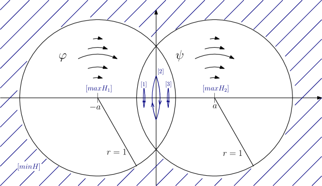
In this section we offer a few examples in which our implementation computes the GF-barcode for a composition of two compactly supported Hamiltonian diffeomorphisms of generated by radial Hamiltonian functions with different centers and the results indeed give good approximation of the conjectured barcode.
Let and and consider the profile function with derivative which is a smooth version of the function depicted in Figure 2 and satisfies .


We denote two center points by and two radial Hamiltonian functions that generate flows compactly supported inside and respectively. Recall that in this case and we call the scaling factor of this example. In order to ensure these diffeomorphisms poses simple generating functions and to enable realistic running time and memory requirements we take .
The diffeomorphism has a trivial fixed point at and has a trivial fixed point at , we denote them as and respectively. Since we treat our domain as the compactification , the diffeomorphisms and also have a common trivial fixed point at denoted by . Furthermore, due to the symmetry of this setup one may also estimate additional fixed points in the overlap of both supports, we think of these fixed points as periodic orbits of the concatenation and number them by their position along the horizontal axis as shown in Figure 3. Note that the total number of periodic orbits depends on the distance and on the scaling factor .
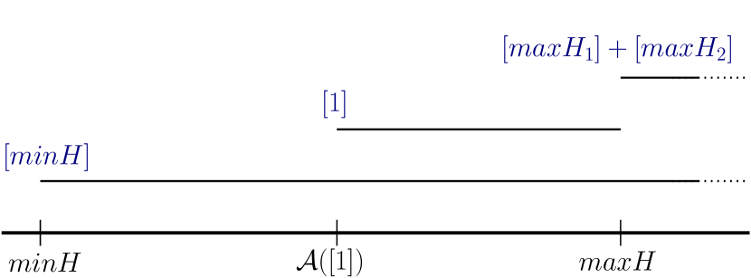
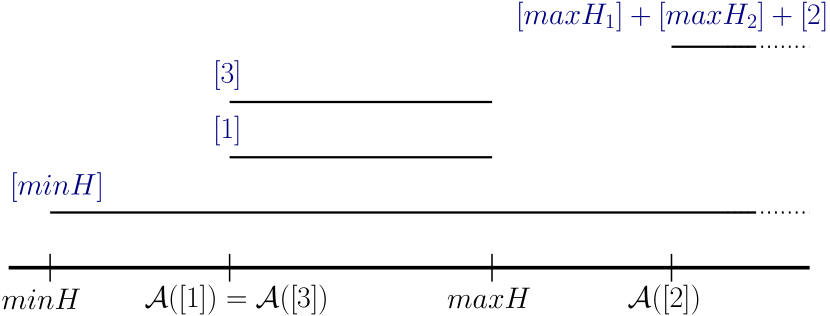
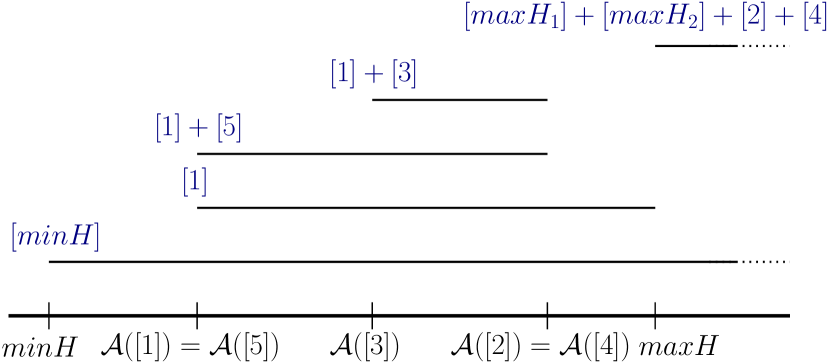
We estimate the actions of each periodic orbit and deduce their Conley-Zehnder indices (see [17, Section 8.1]), then we compile this information into a conjectured barcode for different values of , resulting in possible cases, described in Figure 4. Note that bars correspond to homology classes represented by chains of critical points of the generating function, considered as the fixed points denoted earlier.
Finally, we compute these examples using the suggested implementation of our algorithm with different mesh parameters and scaling factors yielding barcodes whose bottleneck distances to the conjectured barcodes are then measured relative to the scaling factor . The results are given in Table 1 for a specific choice of scaling factor () and mesh parameter () but we mention that these results are consistent through other viable choices of parameters as well.
| Case of | Estimated | ||
| Case II | |||
| Case III | |||
| Case IV | |||
| Case I |
Hence the approximated barcodes are indeed quite accurate and the error in bottleneck distance is actually much smaller than the one given by our theoretical bound in these examples which in all cases was after normalization by the scaling factor .
Remark.
It would be interesting to implement practically our algorithm for larger values of and .
References
- [1] D. Alvarez-Gavela et al. “Embeddings of free groups into asymptotic cones of Hamiltonian diffeomorphisms” In Journal of Topology and Analysis 11.02, 2019, pp. 467–498 DOI: 10.1142/S1793525319500213
- [2] V.I. Arnold “Mathematical methods of classical mechanics” Springer, 1989
- [3] Ulrich Bauer and Michael Lesnick “Induced matchings and the algebraic stability of persistence barcodes” In J. Comput. Geom. 6.2, 2015, pp. 162–191
- [4] Ulrich Bauer, Michael Kerber, Jan Reininghaus and Hubert Wagner “Phat—persistent homology algorithms toolbox” In J. Symbolic Comput. 78, 2017, pp. 76–90 DOI: 10.1016/j.jsc.2016.03.008
- [5] Misha Bialy and Leonid Polterovich “Geodesics of Hofer’s metric on the group of Hamiltonian diffeomorphisms” In Duke Math. J. 76.1, 1994, pp. 273–292 DOI: 10.1215/S0012-7094-94-07609-6
- [6] Marc Chaperon “Phases génératrices en géométrie symplectique” talk:7 In Les rencontres physiciens-mathématiciens de Strasbourg -RCP25 41 Institut de Recherche Mathématique Avancée - Université Louis Pasteur, 1990 URL: http://www.numdam.org/item/RCP25_1990__41__191_0
- [7] Herbert Edelsbrunner and John L. Harer “Computational topology” An introduction American Mathematical Society, Providence, RI, 2010, pp. xii+241
- [8] M. Fraser “Contact spectral invariants and persistence” In Preprint arXiv:1502.05979, 2015
- [9] Allen Hatcher “Algebraic topology” Cambridge University Press, Cambridge, 2002, pp. xii+544
- [10] Lars Hörmander “Fourier integral operators. I” In Acta Math. 127.1-2, 1971, pp. 79–183 DOI: 10.1007/BF02392052
- [11] Asaf Kislev and Egor Shelukhin “Bounds on spectral norms and barcodes” In Geom. Topol. 25.7, 2021, pp. 3257–3350 DOI: 10.2140/gt.2021.25.3257
- [12] François Laudenbach and Jean-Claude Sikorav “Persistance d’intersection avec la section nulle au cours d’une isotopie hamiltonienne dans un fibré cotangent” In Invent. Math. 82.2, 1985, pp. 349–357 DOI: 10.1007/BF01388807
- [13] Dusa McDuff and Dietmar Salamon “Introduction to symplectic topology”, Oxford Graduate Texts in Mathematics Oxford University Press, Oxford, 2017, pp. xi+623 DOI: 10.1093/oso/9780198794899.001.0001
- [14] J. Milnor “Morse theory”, Based on lecture notes by M. Spivak and R. Wells. Annals of Mathematics Studies, No. 51 Princeton University Press, Princeton, N.J., 1963, pp. vi+153
- [15] L. Polterovich, E. Shelukhin and V. Stojisavljević “Persistence modules with operators in Morse and Floer theory” In Mosc. Math. J. 17.4, 2017, pp. 757–786
- [16] Leonid Polterovich and Egor Shelukhin “Autonomous Hamiltonian flows, Hofer’s geometry and persistence modules” In Selecta Mathematica 22.1, 2016, pp. 227–296 DOI: 10.1007/s00029-015-0201-2
- [17] Leonid Polterovich, Daniel Rosen, Karina Samvelyan and Jun Zhang “Topological persistence in geometry and analysis” American Mathematical Soc., 2020
- [18] Egor Shelukhin “On the Hofer-Zehnder conjecture” In Preprint arXiv:1905.04769, 2019
- [19] Jean-Claude Sikorav “Problèmes d’intersections et de points fixes en géométrie hamiltonienne” In Comment. Math. Helv. 62.1, 1987, pp. 62–73 DOI: 10.1007/BF02564438
- [20] Bret Stevenson “A quasi-isometric embedding into the group of Hamiltonian diffeomorphisms with Hofer’s metric” In Israel J. Math. 223.1, 2018, pp. 141–195 DOI: 10.1007/s11856-017-1612-x
- [21] David Théret “Utilisation des fonctions generatrices en geometrie symplectique globale”, 1996
- [22] David Théret “A complete proof of Viterbo’s uniqueness theorem on generating functions” In Topology Appl. 96.3, 1999, pp. 249–266 DOI: 10.1016/S0166-8641(98)00049-2
- [23] Lisa Traynor “Symplectic homology via generating functions” In Geom. Funct. Anal. 4.6, 1994, pp. 718–748 DOI: 10.1007/BF01896659
- [24] Michael Usher and Jun Zhang “Persistent homology and Floer–Novikov theory” In Geom. Topol. 20.6, 2016, pp. 3333–3430 DOI: 10.2140/gt.2016.20.3333
- [25] Claude Viterbo “Symplectic topology as the geometry of generating functions” In Math. Ann. 292.4, 1992, pp. 685–710 DOI: 10.1007/BF01444643
- [26] Claude Viterbo “An introduction to symplectic topology through sheaf theory” In Preprint, 2011
- [27] Jun Zhang “-cyclic persistent homology and Hofer distance” In J. Symplectic Geom. 17.3, 2019, pp. 857–927 DOI: 10.4310/JSG.2019.v17.n3.a7
- [28] Afra Zomorodian and Gunnar Carlsson “Computing persistent homology” In Discrete Comput. Geom. 33.2, 2005, pp. 249–274 DOI: 10.1007/s00454-004-1146-y