Rethinking Visual Geo-localization for Large-Scale Applications

Abstract

Visual Geo-localization (VG) is the task of estimating the position where a given photo was taken by comparing it with a large database of images of known locations. To investigate how existing techniques would perform on a real-world city-wide VG application, we build San Francisco eXtra Large, a new dataset covering a whole city and providing a wide range of challenging cases, with a size 30x bigger than the previous largest dataset for visual geo-localization. We find that current methods fail to scale to such large datasets, therefore we design a new highly scalable training technique, called CosPlace, which casts the training as a classification problem avoiding the expensive mining needed by the commonly used contrastive learning. We achieve state-of-the-art performance on a wide range of datasets and find that CosPlace is robust to heavy domain changes. Moreover, we show that, compared to the previous state-of-the-art, CosPlace requires roughly 80% less GPU memory at train time, and it achieves better results with 8x smaller descriptors, paving the way for city-wide real-world visual geo-localization. Dataset, code and trained models are available for research purposes at https://github.com/gmberton/CosPlace.

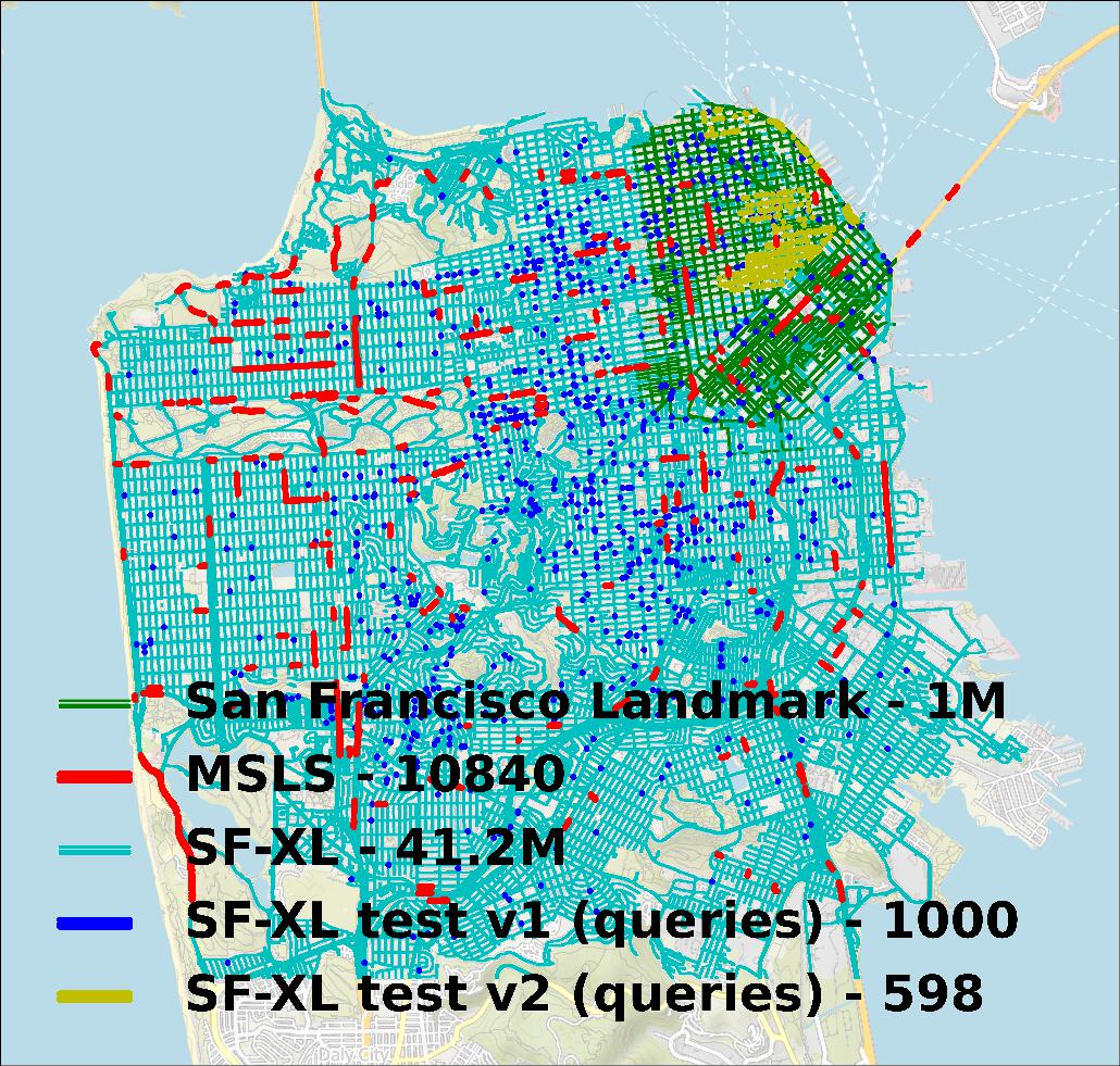
Figure 1: Map of various datasets on the city of San Francisco. Previous datasets only cover a sector of the city (green points) or are sparse (red points). SF-XL densely covers the whole city and provides a realistic case-study for large-scale applications.

1 Introduction

Visual geo-localization (VG), also known as visual place recognition [1] or image localization [32], is a staple of computer vision [47, 1, 46, 15, 21, 48, 54] and robotics research [9, 11, 10, 17, 26, 22] and it is defined as the task of coarsely recognizing the geographical location where a photo was taken, usually with a tolerance of few meters [1, 27, 32, 18, 5, 24, 50]. This task is commonly approached as an image retrieval problem where the query to be localized is compared to a database of geo-tagged images: the most similar images retrieved from the database, together with their metadata, represent the hypotheses of the query’s geographical location. In particular, all recent VG methods are learning-based and use a neural network to project the images into an embedding space that well represents the similarity of their locations, and that can be used for the retrieval.

So far, research on VG has focused on recognizing the location of images in moderately sized geographical areas (e.g., a neighborhood). However, real-world applications of this technology, such as autonomous driving [15] and assistive devices [12], are posed to operate at a much larger scale (e.g., cities or metropolitan areas), thus requiring massive databases of geo-tagged images to execute the retrieval. Having access to such massive databases, it would be advisable to use them also to train the model rather than just for the execution of the retrieval (inference). This idea requires us to rethink VG, addressing the two following limitations.

Non-representative datasets. The current datasets for VG are not representative of realistic large-scale applications, because they are either too small in the geographical coverage [1, 46, 34, 19, 7] or too sparse [50, 13, 33, 2] (see Fig. 1 for an example of these limitations). Moreover, current datasets follow the common practice of splitting the collected images into geographically disjoint sets for training and inference. However, this practice does not find a correspondence in the real world where one would likely opt to use images from the target geographical area to train the model. Considering also the cost of collecting the images, it would be advisable to use the whole database also for training.

Scalability of training. Having access to a massive amount of data raises the question of how to use it effectively for training. All the recent state-of-the-art methods in VG use contrastive learning [1, 27, 18, 32, 50, 21, 37, 36, 5, 24] (mostly relying on a triplet loss), which heavily depends on mining of negative examples across the training database [1]. This operation is expensive, and it becomes prohibitive when the database is very large. Lightweight mining strategies that explore only a small pool of samples can reduce the duration of the mining phase [50], but they still result in a slow convergence and possibly less effective use of the data.

Contributions. In this paper, we address these two limitations with the following contributions:

• A new large-scale and dense dataset, called San Francisco eXtra Large (SF-XL), that is roughly 30x bigger than what is currently available (see Fig. 1). The dataset includes crowd-sourced (i.e., multi-domain) queries that make for a challenging problem.

• A procedure that uses a classification task as a proxy to train the model that is used at inference to extract discriminative descriptors for the retrieval. We call this method CosPlace. CosPlace is remarkably simple, it does not necessitate to mine negative examples, and it can effectively learn from massive collections of data.

Through extensive experimental validation, we demonstrate that not only CosPlace requires roughly 80% less GPU memory at train time than current SOTA, but also that a simple model trained with CosPlace on SF-XL surpasses the SOTA while using 8x smaller embeddings. Additionally, we show that this model generalizes far better to other datasets.

2 Related work

Visual geo-localization as image retrieval. Visual geo-localization is commonly approached as an image retrieval problem, with a retrieved image deemed correct if it is within a predefined range (usually 25 meters) from the query’s ground truth position [1, 27, 32, 18, 5, 50]. All recent VG methods perform the retrieval using learned embeddings that are produced by a feature extraction backbone equipped with a head that implements some form of aggregation or pooling, the most notable being NetVLAD [1]. These architectures are trained via contrastive learning, typically using a triplet loss [1, 27, 50, 21, 37, 36, 5, 24] and leveraging the geo-tags of the database images as a form of weak supervision to mine negative examples [1]. There are various alternatives to this scheme, such as the Stochastic Attraction-Repulsion Embedding (SARE) loss [32], which allows to efficiently use multiple negatives at once, while keeping the training methodology from [1]. Another solution is presented in [18], and it achieves new state-of-the-art results by computing the loss not only over the full images but also over cleverly mined crops. Despite the variations, all these methods suffer from poor train-time scalability caused by expensive mining techniques. The problem of scalability also arises at test time, and it relates to the size of the descriptors, which impacts the required memory and the retrieval time. Although the dimensionality of NetVLAD descriptors can be reduced using PCA, this leads to a degradation of results  [1], hence works like [18, 32] prefer to keep a high dimensionality of 4096. Alternatively, other works drop NetVLAD and instead use pooling [40] to build smaller embeddings.

Visual geo-localization as classification. An alternative approach to visual geo-localization is to consider it a classification problem [52, 42, 35, 25, 30]. These works build on the idea that two images coming from the same geographical region, although representing different scenes, are likely to share similar semantics, such as architectural styles, types of vehicles, vegetation, etc. In practice, these methods divide the geographical area of interest in cells and group the database of images in classes according to their cell. This formulation allows to scale the problem to the whole globe, but at the cost of reduced accuracy in the estimates because each class can span many kilometers. Therefore, these methods are not used to perform geo-localization when the estimates require tolerance of a few meters.

Relation to prior works. In this work, we propose a new approach to VG that combines the advantages of both retrieval (tolerance of a few meters) and classification (high scalability). Our method uses a classification task as a proxy to train the model without requiring any mining. This makes it possible to train with massive datasets, unlike the solutions that use contrastive learning [1, 27, 50, 21, 37, 36, 5, 24]. At test time, the trained model is used to extract image descriptors and perform a classic retrieval. While CosPlace might appear similar to previous classification-based works [52, 42, 35, 25, 30], given that they also partition a map into classes, there are substantial differences. These prior works tackle the task of global classification and group images within very large cells (up to hundreds of kilometers wide), building on the idea that nearer scenes have similar semantics (e.g. if two images are from China, they might both depict Chinese ideograms). On the other hand, our partitioning strategy is designed to leverage the availability of dense data and ensure that if two images are from the same class, they visualize the same scene. Moreover, unlike [52, 42, 35, 25, 30], once trained our method can be used to perform geo-localization through image retrieval on any given geographical area.

3 The San Francisco XL dataset

There are numerous datasets for VG (see Tab. 1), but none of them reflects the scenario in which the geo-localization must be performed in a large environment and with few meters of tolerance: some datasets are limited to a small geographical area [1, 46, 5, 7] whereas others do not densely cover the area [50, 19, 13, 33, 2, 41]. The San Francisco Landmark Dataset [8] partially overcomes these limitations, but it does not cover the whole city, nor has long-term temporal variations, which are essential for robustly training a neural network [1]. Here we propose the first city-wide, dense, and temporally variable dataset: San Francisco eXtra Large (SF-XL).

Dataset # images Scenario Appearance Changes Dense Coverage 6 DoF Poses Urban Suburban Weather Long-term Day/Night Intrinsics KITTI [19] 13k ✓ ✓ ✗ ✗ ✗ ✗ ✗ ✓ Eynsham [13] 48k ✓ ✓ ✗ ✗ ✗ ✗ ✗ ✗ St Lucia [34] 33k ✗ ✓ ✗ ✗ ✗ ✗ ✓ ✗ NCLT [7] 3.8M ✓ ✗ ✗ ✗ ✗ ✗ ✓ ✓ Oxford RobotCar [33] 27k ✓ ✓ ✓ ✓ ✓ ✗ ✗ ✓ CMU [2] 128k ✓ ✓ ✓ ✓ ✗ ✗ ✗ ✓ Pittsburgh250k [1] 278k ✓ ✗ ✗ ✓ ✗ ✗ ✓ ✗ TokyoTM/247 [46] 189k ✓ ✗ ✗ ✓ ✓ ✓ ✓ ✗ MSLS [50] 1.7M ✓ ✓ ✓ ✓ ✓ ✓ ✗ ✗ San Francisco Landmark [8] 1.1M ✓ ✗ ✗ ✗ ✗ ✓ ✓ ✓ Aachen [41] 4k ✓ ✗ ✗ ✗ ✓ ✓ ✗ ✓ SF-XL (Ours) 41.2M ✓ ✓ ✓ ✓ ✓ ✓ ✓ ✓

Table 1: Comparison of various VG datasets.

Database. Like other datasets used in this task [1, 46, 5, 29, 55, 56], SF-XL’s database is created from Google StreetView imagery. We collected 3.43M equirectangular panoramas (360° images) and split them horizontally in 12 crops, following [46, 1]. This results in a total of 41.2M images (some examples are presented in Fig. 9). Each crop is labeled with 6 DoF information (which includes GPS and heading). The images were taken between 2009 and 2021, thus providing an abundance of long-term temporal variations.

Besides scale and density, SF-XL differs from previous datasets [1, 46, 50, 5] in that the database is not split in geographically non-overlapping subsets for training, validation and testing. We argue that such division of the database does not reflect the reality of applications that may use VG. In fact, when tasked with building a VG application for a large geographical area, one would likely opt to train a neural network on the imagery of such area rather than additionally collecting images from a disjointed one (perhaps adjacent).

To this end, we use the 41.2M images as a training set, which therefore covers the whole area of San Francisco. While at test time, we could use the whole database of 41.2M images for the retrieval, this would be prohibitive for research purposes because extracting the descriptors for all the images on a single GPU requires days. Therefore, we use as test time database only the 2.8M images from the year 2013, which still cover the whole SF-XL geographical area, We found this choice to be a good solution because the set of images is small enough to be a feasible research option for testing but large enough to simulate a real-world scenario and prevent the bad practice of validating or tuning hyperparameters on the test set (as it would take too long to validate on it every epoch).

Finally, for validation, we use a small set of images scattered through the whole city, made of 8k database images and 8k queries.

Queries. While previous methods require the train set to be split into database and queries, CosPlace does not need this distinction. For this reason, we release the training set as a whole, and we believe that methods relying on database/queries splits for training (e.g., [1, 27, 32, 18, 37, 36, 53]) should choose the split that best suits their needs, given that this choice can heavily influence the results (see in Tab. 3 the difference in results between the third and fourth row as an example of this phenomenon).

SF-XL SF-XL SF-XL test v1 SF-XL test v2 (Train) (Val) (Test) (Test) Database 41.2M 8k 2.8M 2.8M Queries 8k 1000 598

Table 2: Number of images for each subset of SF-XL. The train set is not split into database and queries.

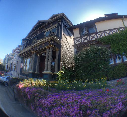
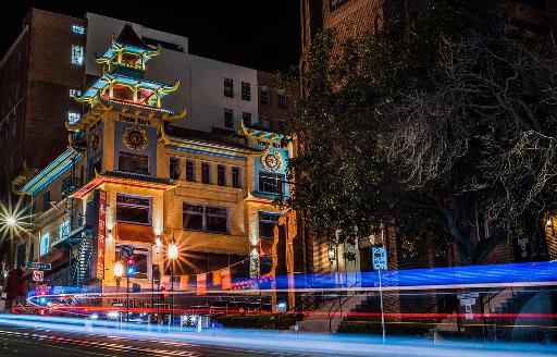
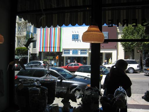
Figure 2: Examples of queries from SF-XL’s test set v1

Concerning the test queries, we believe that they should not be from the same domain as the database, because in most real-world scenarios test time queries could come from unseen domains. This is also in agreement with what is done in the San Francisco Landmark Dataset [8] and Tokyo 24/7 [46]. Hence, in SF-XL we include two different sets of test queries:

• test set v1: a set of 1000 images collected from Flickr (similarly to Oxford5k [38], Paris6k [39], Sfm120k [40]). Given the inaccurate GPS coordinates of Flickr imagery, all the images in this set were hand-picked, and their location has been manually verified. We also made sure to blur out faces and plate numbers to anonymize the pictures. These images are very diverse and have a wide range of viewpoint and illumination (day/night) changes (see Fig. 2);

• test set v2: a set of 598 images from the queries of the San Francisco Landmark Dataset [8], for which the 6 DoF coordinates have been generated by [48]. Given that it provides 6 DoF labels, this set can also be used for large-scale pose estimation.

Tab. 2 presents a summary of SF-XL, while further information about it are in Appendix A.

4 Method

Given that a city-wide dataset requires millions of images (Sec. 3) and that visual geo-localization is by nature a large-scale task, we believe that a proper method for VG should be highly scalable, both at train and at test time. We find that current (and previous) state of the art [1, 27, 32, 18] lacks these important qualities:

• at train time, they require to periodically compute the features of all database images and keep them in a cache: this results in a space and time complexity of $\mathcal{O}(n)$, which is suitable only for small datasets;

• these methods [1, 27, 32, 18] rely on a NetVLAD layer [1] or its variants [27], which produce high dimensional vectors and require large amounts of memory for inference (given that database descriptors should be kept in memory for efficient retrieval). As an example, a VGG-16 with NetVLAD produces vectors of dimension 32k, which for a 10M database would require $32\text{k}\cdot 10\textrm{M}\cdot 4\textrm{B}=1220\textrm{GB}$ of memory. Smaller embeddings are usually obtained with reduction techniques such as PCA, although using dimensions lower than 4096 leads to a rapid decline of results [1, 37, 36, 57].

To reduce train time complexity we take inspiration from the domain of face recognition, where cosFace [49] and arcFace [14] are key in achieving state-of-the-art results [44]. These losses require the training set to be divided into classes; however, in VG the label space is continuous (GPS coordinates and optionally heading/orientation information), making it not straightforward to divide it into discrete classes.

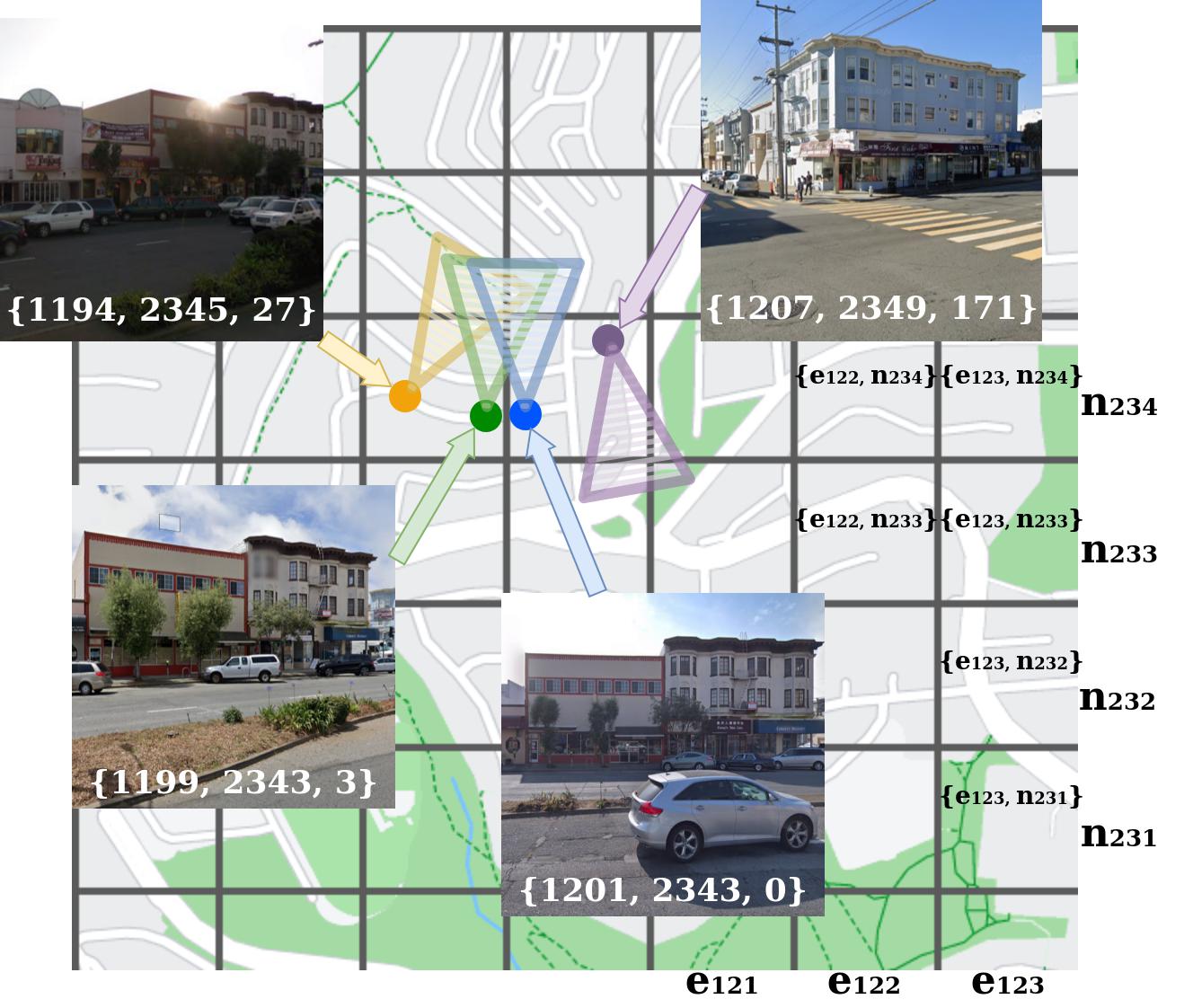
Figure 3: Grid of the map showing how cells are formed based on UTM coordinates. Each cell (of side lenght $M$) is identified by a pair of values (for readability only a few are shown on the right). On each of the four images is written its triplet $\{\textit{UTM east},\textit{UTM north},\textit{heading}\}$ in white between braces. Within any given cell there are images with very different headings/orientations (see the two images on the right), which should belong to different classes, hence the split of each cell into multiple classes according to their heading. We also see that the two images at the bottom, although representing the same scene/building, belong to different cells (and therefore to different classes), and this would be confusing for a naive classification-based algorithm.

4.1 Splitting the dataset into classes

A naive approach to divide the database into classes would be to split it into square geographical cells (see Fig. 3), using UTM coordinates $\{\textit{east},\textit{north}\}$, and further slice each cell into a set of classes according to each image’s orientation/heading $\{\textit{heading}\}$. Formally, the set of images assigned to the class $C_{e_{i},n_{j},h_{k}}$ would be

where $M$ and $\alpha$ are two parameters (respectively in meters and degrees) that determine the extent of each class in position and heading. While this solution creates a set of classes from a VG dataset, it has a big limitation: nearly identical images (e.g., taken with the same orientation but a few centimeters apart) may be assigned to different classes due to quantization errors (see Fig. 3), which would confuse a classification-based training algorithm.

To overcome this limitation, we propose not to train the model using all the classes at once, but just groups of non-adjacent classes (two classes are adjacent if an infinitesimal difference in position or heading can bring an image from one class to the other). Intuitively, these groups, which we call CosPlace Groups, are akin to separate datasets and our proposed training procedure (explained later in Sec. 4.2) iterates over them, one at a time. We generate groups by fixing the minimum spatial separation that two classes of the same group should have, either in terms of translation or orientation. For this purpose, we introduce two hyperparameters: $N$ controls the minimum number of cells between two classes of the same group, and $L$ is the equivalent for the orientation (see Fig. 4 for a visual description). Formally, we define the CosPlace Group $G_{uvw}$ as the set of classes defined as follows

$$\scalebox{0.95}{$G_{uvw}$} =\big{\{}C_{e_{i}n_{j}h_{k}}:(e_{i}\bmod N=u)\;\land$$ (2)

$$\land\;(n_{j}\bmod N=v)\land\left(h_{k}\bmod L=w\right)\big{\}}$$

By construction, CosPlace Groups are disjoint sets of classes from Eq. 1 with the following properties:
Property 1: each class belongs to exactly one group.
Property 2: within a given group, if two images belong to different classes they are at least $M\cdot(N-1)$ meters apart or $\alpha\cdot(L-1)$ degrees apart (see Fig. 4);
Property 3: the total number of CosPlace Groups is $N\times N\times L$.
Property 4: no two adjacent classes can belong to the same group (unless $N=1$ or $L=1$).

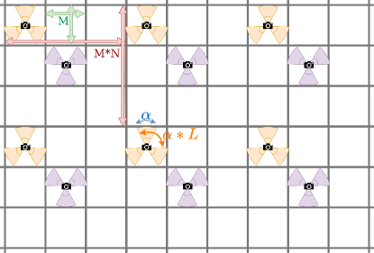
Figure 4: Visual representation of CosPlace groups. The orange triangles represent one of the $N\times N\times L$ different groups, while the purple triangles represent another group. For clarity, only two groups are shown (namely $G_{000}$ and $G_{111}$). Each triangle represents one class, which contains all images within the respective cell with the proper orientation. The meaning for each of the four hyperparameters that define how groups are built (i.e., $M$, $\alpha$, $N$ and $L$) is visually shown. In the figure, $\alpha=60\degree,N=3,L=2$. The total number of groups with this configuration is therefore $3\times 3\times 2=18$, and each cell contains 6 classes from 2 groups.

4.2 Training the network

We will now describe how the CosPlace Groups are used to train the model. We take inspiration from the Large Margin Cosine Loss (LCML) [49] also known as cosFace [49, 44, 51], which has shown remarkable results in face recognition [44] and landmark retrieval [51]. Nonetheless, vanilla LCML cannot be applied directly to any VG dataset, given that images are not split into a finite number of classes. However, with the proposed partitioning of the dataset, we can perform LCML sequentially over each CosPlace group (where each group can be considered as a separate dataset) and iterate over the many groups. We call this training procedure CosPlace. As the LCML relies on a fully connected layer with output dimensionality equal to the number of classes, CosPlace requires one fully connected layer per group: these layers are then discarded for validation/test. Note that not all groups must necessarily be used for training, as one could simply use a single group and ignore the others; however, the full ablation at Fig. 10 shows that using more than one group helps achieve better results. Therefore, we train sequentially over the groups. Formally, for each group:

$$\mathcal{L}_{\textit{cosPlace}}=\mathcal{L}_{\textit{lmcl}}(G_{uvw})$$ (3)

where $\mathcal{L}_{\textit{lmcl}}$ is the LCML loss as defined in [49], $u\in\{0,\ldots,N\}$, $v\in\{0,\ldots,N\}$, $W\in\{0,\ldots,L\}$. In practice, we train one epoch on $G_{000}$, the next one on $G_{001}$, and so on, iterating over the groups. The remarkable advantage of this procedure w.r.t. the methods based on contrastive losses commonly used in visual geo-localization, is that no mining nor caching is required, making it a much more scalable option. At validation and test time, we use the model not to classify the query, but rather to extract image descriptors as in [49] for a classic retrieval over the database. This allows for the model to be used also on other datasets from unseen geographical areas (see Tab. 3).

5 Experiments

5.1 Implementation details

Architecture. CosPlace is architecture-agnostic, i.e. it can be applied on virtually any image-based model. For most experiments, we rely on a simple network made of a standard CNN backbone followed by a GeM pooling and a fully connected layer with output dimension 512. Note that such a simple architecture is in contrast with the trend of the last five years of research in Visual Geo-localization [1, 27, 32, 18, 37, 53, 36], where the architectures rely on a more complex (w.r.t. our architecture) NetVLAD layer [1], and some even add a number of blocks on top of it [27, 37, 36], resulting in heavier and slower architectures. Given that previous methods rely on a VGG-16 backbone [1, 27, 32, 18, 37, 36, 53, 57], we use a VGG-16 in Sec. 5.2, for fair comparisons with other methods. For our ablations and preliminary experimentations, we relied on a ResNet-18, which achieves similar results to the VGG-16 at a fraction of the training time and memory requirements. In Fig. 5 and Sec. B.3.1, we investigate the use of more recent backbones (ResNets [23] and transformer-based [16, 20]) with varying output dimensionality, finding that CosPlace reaches encouraging results with a wide variety of architectures and thus demonstrates a great flexibility. For example, we find that CosPlace with a ResNet-101 backbone and 128-D descriptors outperforms current SOTA, which uses 4096-D descriptors.

Training. Regarding hyperparameters, we set $M=10$ meters, $\alpha=30\degree$, $N=5$ and $L=2$. We define an epoch as 10k iterations over a group. We perform an epoch over the first group, then an epoch over the second group and so on, for a total of 50 epochs (i.e., 500k iterations with batch size of 32). To ensure that the same group is seen more than once during training, we use only 8 of the $N\times N\times L$ (i.e., $5\times 5\times 2=50$) groups. Validation is performed after each epoch, and once training is finished, testing is performed using the model that obtained the best performance on the validation set. In Sec. B.2, we provide further implementation details, and we discuss how CosPlace not only reduces the number of hyperparameters in comparison to previous VG methods but also that the ones it introduces have an intuitive meaning (see Fig. 4).

With respect to NetVLAD-based methods [1, 27, 32, 18, 37, 53, 36], which represent the entirety of the state of the art of the past five years, our method does not require multiple steps, whereas the NetVLAD layer requires for features clusters to be computed before starting to train the network, and, optionally, PCA to be computed afterwards.

5.2 Comparison with other methods

In this section, we compare CosPlace with previous methods in visual geo-localization. For a proper assessment of the results, we test on 7 datasets, namely Pitts250k [1], Pitts30k [1], Tokyo 24/7 [46], St Lucia [34], Mapillary Street Level Sequences (MSLS) [50], and our proposed SF-XL test v1 and SF-XL test v2. Of these datasets, MSLS and St Lucia are composed of frontal view images taken with cars, while the rest rely on Google StreetView imagery to build the database. For MSLS, given that the test set labels have not been publicly released yet, we test on the validation set as in [21, 4]. As a metric, we use the recall@N with a 25 meters threshold, i.e., the percentage of queries for which at least one of the first N predictions is within a 25 meters distance from the query, following standard procedure [1, 27, 32, 18, 5, 21, 3, 50].

We perform experiments with NetVLAD [1], CRN [27], GeM [40], SARE [32] and SFRS [18]. These methods are trained on the popular Pitts30k [1] dataset, and we apply color jittering for all, following SFRS. Although for some of them, it is intractable to train on a large-scale dataset such as MSLS or SF-XL (e.g., SFRS’s code relies on pairwise distance computation in features space between any pair of query-database image, which makes space and time complexity grow quadratically with the number of images), we are able to train GeM and NetVLAD also on MSLS and SF-XL using the partial mining from [50], which scales to larger datasets. With this mining technique, we perform training with two different database/queries splits of SF-XL (note that previous methods, unlike CosPlace, require the dataset to be split): SF-XL* uses images after 2010 as queries, and the rest as database, while SF-XL** uses images after 2015 as queries and before 2015 as database (resulting in a denser database). We also report results with other methods such as SPE-VLAD [53], SRALNet [36], APPSVR [37] and APANet [57], although the code for these works is not publicly available and we could not independently reproduce the results.

Method Desc. dim. Train set Pitts250k Pitts30k Tokyo 24/7 MSLS St Lucia Average R@1 R@5 R@1 R@5 R@1 R@5 R@1 R@5 R@1 R@5 R@1 R@5 NetVLAD [1] 32768 Pitts30k 85.9$\pm$ 0.3 93.6$\pm$ 0.2 86.1$\pm$ 0.1 94.1$\pm$ 0.3 62.2$\pm$ 0.7 75.4$\pm$ 0.5 54.8$\pm$ 1.1 66.6$\pm$ 1.0 70.8$\pm$ 0.5 81.8$\pm$ 0.7 72.0 82.3 NetVLAD [1] 32768 MSLS 79.7$\pm$ 0.8 90.2$\pm$ 0.9 80.9$\pm$ 1.4 90.6$\pm$ 1.2 63.6$\pm$ 1.1 77.5$\pm$ 1.2 75.4$\pm$ 0.4 84.2$\pm$ 0.2 92.8$\pm$ 0.4 97.6$\pm$ 0.3 78.5 88.0 NetVLAD [1] 32768 SF-XL* 81.5$\pm$ 0.1 90.8$\pm$ 0.3 82.1$\pm$ 0.2 91.5$\pm$ 0.2 66.3$\pm$ 0.4 78.2$\pm$ 0.5 59.3$\pm$ 0.8 68.7$\pm$ 0.7 80.6$\pm$ 0.5 90.7$\pm$ 0.8 74.0 84.0 NetVLAD [1] 32768 SF-XL** 76.2$\pm$ 0.3 88.8$\pm$ 0.4 78.8$\pm$ 0.4 90.0$\pm$ 0.4 56.2$\pm$ 0.8 67.7$\pm$ 0.9 51.4$\pm$ 0.9 60.7$\pm$ 0.7 78.5$\pm$ 0.6 88.3$\pm$ 0.8 68.2 79.1 CRN [27] 32768 Pitts30k 87.0$\pm$ 0.4 94.5$\pm$ 0.1 86.3$\pm$ 0.4 94.6$\pm$ 0.4 62.8$\pm$ 0.5 77.4$\pm$ 0.8 57.6$\pm$ 0.3 70.4$\pm$ 0.8 70.9$\pm$ 0.7 82.8$\pm$ 0.7 72.9 83.9 SPE-VLAD [53] † 32768 Pitts30k - - - 89.2 - 63.9 - - - - - - SARE [32] 4096 Pitts30k 88.0$\pm$ 0.6 94.8$\pm$ 0.3 87.2$\pm$ 0.8 93.9$\pm$ 0.3 74.8$\pm$ 3.0 84.3$\pm$ 1.6 62.4$\pm$ 2.9 73.2$\pm$ 2.8 72.7$\pm$ 2.6 86.0$\pm$ 2.0 77.0 86.4 SFRS [18] 4096 Pitts30k 90.1$\pm$ 0.3 95.8$\pm$ 0.2 88.7$\pm$ 0.3 94.2$\pm$ 0.1 78.5$\pm$ 0.8 87.3$\pm$ 0.5 62.8$\pm$ 0.8 73.0$\pm$ 0.8 72.5$\pm$ 3.6 85.4$\pm$ 3.2 78.5 87.1 SRALNet [36] † 4096 Pitts30k 87.8 94.8 - - 72.1 83.2 - - - - - - APPSVR [37] † 4096 Pitts30k 88.8 95.6 87.4 94.3 77.1 85.7 - - - - - - GeM [40] 512 Pitts30k 75.3$\pm$ 0.2 88.4$\pm$ 0.3 77.9$\pm$ 0.4 90.5$\pm$ 0.3 46.4$\pm$ 0.9 65.3$\pm$ 0.7 51.8$\pm$ 0.9 64.4$\pm$ 0.9 59.9$\pm$ 1.6 76.3$\pm$ 2.0 62.3 77.0 GeM [40] 512 MSLS 65.3$\pm$ 1.2 81.0$\pm$ 1.6 71.6$\pm$ 2.1 85.1$\pm$ 1.9 44.9$\pm$ 1.7 62.6$\pm$ 1.2 66.7$\pm$ 0.7 78.9$\pm$ 0.5 84.6$\pm$ 1.1 93.3$\pm$ 0.7 66.6 80.2 GeM [40] 512 SF-XL* 64.7$\pm$ 0.8 81.4$\pm$ 0.8 67.8$\pm$ 0.6 83.6$\pm$ 0.7 37.9$\pm$ 2.3 51.0$\pm$ 2.1 46.8$\pm$ 2.1 58.1$\pm$ 1.2 68.5$\pm$ 2.4 82.7$\pm$ 1.8 57.1 71.4 APANet [57] † 512 Pitts30k 83.7 92.6 - - 67.0 81.0 - - - - - - CosPlace (Ours) 512 SF-XL 89.7$\pm$ 0.0 96.4$\pm$ 0.2 88.5$\pm$ 0.2 94.5$\pm$ 0.0 82.8$\pm$ 0.9 90.0$\pm$ 0.6 79.5$\pm$ 0.1 87.2$\pm$ 0.2 94.3$\pm$ 0.4 97.4$\pm$ 0.3 87.0 93.1

Table 3: Comparisons of various methods on popular datasets. Two values of recalls are used as metric (R@1, R@5), with threshold distance for positives of 25 meters. Results rely on a CNN with a VGG-16 backbone, and are averaged over 3 runs with seeds 0, 1 and 2. * images taken after 2010 are used as queries, and the rest as database. ** images taken after 2015 are used as queries, and the rest as database. †these results could not be independently verified given that no public code implementation is available and we were unable to reproduce the results. The results (when available) were taken from the respective papers.

Method Desc. dim. Train set SF-XL test v1 SF-XL test v2 R@1 R@5 R@10 R@1 R@5 R@10 NetVLAD [1] 32768 Pitts30k 40.0 48.8 52.8 71.1 82.4 84.8 NetVLAD [1] 32768 MSLS 22.9 32.0 37.1 48.2 64.7 69.7 NetVLAD [1] 32768 SF-XL* 38.3 47.4 51.7 70.7 83.4 87.0 NetVLAD [1] 32768 SF-XL** 28.4 38.6 43.1 60.9 74.6 78.6 CRN [27] 32768 Pitts30k 45.8 56.9 60.7 76.4 85.3 87.8 SARE [32] 4096 Pitts30k 45.5 56.5 60.0 78.8 87.6 90.5 SFRS [18] 4096 Pitts30k 51.2 62.2 66.6 83.1 90.5 93.5 GeM [40] 512 Pitts30k 21.7 30.3 34.4 43.1 63.7 69.2 GeM [40] 512 MSLS 8.1 15.6 20.2 29.3 46.3 53.8 GeM [40] 512 SF-XL* 9.8 17.6 21.2 34.8 55.5 63.0 CosPlace (Ours) 512 SF-XL 64.7 73.3 76.6 83.4 91.6 94.1

Table 4: Comparisons on SF-XL test v1 and SF-XL test v2.

Discussion of results. Results are reported in Tab. 3 and Tab. 4, and all rely on VGG-16-based architectures. The results can be summarized in a few points:
- CosPlace achieves best results on average, outperforming the second-best method by 8.5% of R@1 averaged over five datasets.
- CosPlace shows strong robustness to datasets coming from other sources. On the other hand, other methods either perform well on datasets with StreetView-sourced database (i.e., Pitts30k, Pitts250k, Tokyo 24/7) or on datasets with frontal view images (i.e., MSLS and St Lucia). For example, the best performing method on MSLS and St Lucia, namely NetVLAD trained on MSLS, falls short of 10.0% of recall@1 on Pitts250k w.r.t. CosPlace; similarly, the best performing on Pitts30k, namely SFRS trained on Pitts30k, is outperformed by CosPlace by 21.8% on St Lucia.
- While other methods fail to reach competitive results with compact descriptors, we find that CosPlace reaches state-of-the-art with 512-D outputs, paving the way for scalable, robust, and efficient real-world applications. In Sec. B.3.2, we provide additional results by applying PCA to high-dimensionality descriptors.
- Methods besides CosPlace do not benefit from training on SF-XL. This is likely due to the partial mining [50] (given that standard mining [1] is unfeasible on a large scale).
- For methods other than CosPlace, the way database and queries are partitioned in the training set makes a big difference: training on SF-XL* versus SF-XL**, which use different database/queries partitions, achieve quite different results. This is not a problem for CosPlace since it does not need a database/queries split for training.

Fairness of comparisons. While it can be argued that comparisons in Tab. 3 and Tab. 4 are not fair, given that most other methods are trained on Pitts30k, and CosPlace on a much larger dataset, we want to point out that i) CosPlace cannot be trained on Pitts30k nor MSLS (given that they lack heading labels), and ii) training previous state-of-the-art methods [32, 18] on SF-XL would require a huge amount of resources, and it is practically unfeasible: computing the cache (which contains all database and queries descriptors) involves a forward pass on 40M images, with a memory requirement of 5TB, and it would have to be computed periodically every 1000 iterations.

With these considerations in mind, we were able to use the partial mining method from [50] to train GeM and NetVLAD, which have already been shown to perform competitively with such mining [50], whereas more modern techniques, such as SARE [32] or SFRS [18], cannot be used with partial mining without requiring significant changes to their algorithm. However, the fact that GeM and NetVLAD do not benefit from training on the larger scale of SF-XL proves that our superior results do not come simply from the dataset size and that the proposed algorithm is needed to succeed in city-wide geo-localization.

Moreover, following [1, 27, 32, 18, 37, 36, 53] we did not use as comparisons re-ranking based methods [21, 6, 3, 45], given that they perform an extra post-processing step, while methods like CosPlace simply rely on a more efficient retrieval through a nearest neighbor search.

5.3 Computational efficiency

Train-time memory footprint. Compared to previous methods that use a triplet loss and require to keep the descriptors for each image [1, 32, 18] (or a large number of them [50]) in a cache, CosPlace circumvents this by posing the problem as a classification task without mining/caching. This effectively means that it can scale to very large datasets, whereas previous works [1, 32, 18, 53, 37, 36] would require massive amounts of memory to train on large-scale datasets. Note that a cache for a large dataset could be extremely memory demanding: NetVLAD descriptors for an image weigh about $32\textrm{k}\cdot 4\textrm{B}=128\textrm{KB}$, while a JPEG image of dimension $480\times 640$ is about 70KB; therefore, the cache for a whole dataset is almost twice as heavy as the dataset itself.

GPU requirements. While previous state of the art (i.e., SFRS [18]) requires four 11GB GPUs to train, CosPlace is much lighter. Using the same backbone (a VGG-16 [43]), we only require 7.5 GB on a single GPU to obtain the results shown in Tab. 3 and Tab. 4.

Descriptors dimension. Since the advent of the groundbreaking NetVLAD paper [1], state of the art relied on the NetVLAD layer [1, 27, 32, 18], which produces high-dimensional descriptors. Considering that the compactness of the descriptors is perhaps one of the most important factors when choosing an algorithm in the real world (given that for efficient retrieval, all database descriptors should be kept in memory), we produce much more compact vectors w.r.t. previous methods. For instance, while [1, 27] use the full NetVLAD dimension of 32k, and [32, 18] reduce it to 4k, CosPlace achieves SOTA results with a dimension of just 512. Moreover, in Fig. 5 and Sec. B.3.1, we investigate how results depend on the dimensionality of the descriptors (and the underlying backbones), showing that CosPlace with a ResNet-101 and 128-D descriptors outperforms previous SOTA.

Training and testing speed. The network takes roughly one day to train on SF-XL, similarly to SFRS’s [18] training time on Pitts30k. At test time, with a VGG-16-based model, a V100 GPU is able to extract descriptors for 80 images per second, although we find that the speed largely depends on the backbone and is very similar among the methods of Tab. 3, given that all rely on a VGG-16. However, for large-scale datasets, the time required for the k-Nearest Neighbors search dwarfs the extraction time (considering a real-world scenario where database descriptors are extracted offline). Given that exhaustive kNN’s execution time linearly depends on the dimensionality of the descriptors, our 512-D network is 8 times faster than 4096-D SFRS for inference on large datasets and 64 times faster than 32k-D NetVLAD.

M (meters) $\alpha$ (degrees °) N L SF-XL val set 10 360 1 1 85.8 10 360 5 1 88.5 10 30 5 1 88.2 10 30 1 2 77.1 10 30 5 2 90.9

Table 5: Ablation. Recall@1 with varying values of hyperparameters $M$, $\alpha$, $N$ and $L$. The bottom row represents CosPlace, and the other rows represent CosPlace without some components: for example using $\alpha=360\degree$ means that heading labels are not used (i.e. all images within any given cell belong to the same class); similarly using $N=1$ and $L=1$ means that all classes belong to the same group (and only one group exists, resulting in no group separation). A more thorough ablation is in the appendix.

5.4 Ablation

Hyperparameters. To better understand how the choices made in Sec. 4 impact the results, we perform a series of experiments, reported in Tab. 5. The results show that any naive split of the dataset into classes fails to achieve competitive results. The fact that the last row (which represents the only experiment computed without any intra-group adjacent classes) achieves considerably better results than the other rows clearly proves the benefit of using CosPlace groups.

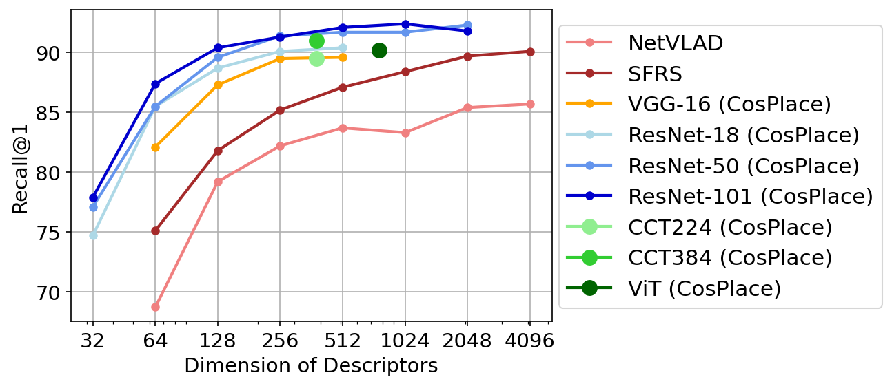
Figure 5: Results on Pitts250k of CosPlace using different backbones and dimensionality of descriptors, compared with SFRS and NetVLAD trained on Pitts30k.

Backbones and descriptors dimensionality. In Fig. 5, we explore the use of different backbones, such as ResNets [23] and Transformers [16, 20]. We find that CosPlace performs well with a variety of backbones, with no need to apply any changes to hyperparameters or layers. This is in contrast with NetVLAD-based architectures (e.g. ResNets followed by NetVLAD perform best when the backbone is cropped at the fourth residual layer instead of the last one [4]). Given that, when using CosPlace, ResNets outperform the VGG-16 while generally being faster and requiring less memory, we believe that future works should move away from the outdated use of VGG-16 backbones towards more efficient ResNets. More details and results on different backbones and descriptors dimensionality are in Sec. B.3.1.

5.5 Limitations

Heading labels. Unlike previous VG methods, which solely rely on GPS/UTM coordinates, we also take advantage of heading labels. This is a drawback of CosPlace, although we argue that heading labels are really inexpensive, and just like GPS coordinates, they can be collected simply through a sensor, without requiring any manual annotation whatsoever. However, some commonly used datasets such as Pitts30k and MSLS do not provide heading labels for their images, making CosPlace not trainable on such datasets.

# images Pitts250k Pitts30k Tokyo 24/7 MSLS St Lucia 5.6M 90.4 89.5 81.6 81.8 98.8 120k 86.0 85.9 67.9 73.3 96.7 12k 82.1 82.9 61.3 66.2 91.2 1.2k 73.3 75.9 45.7 55.0 85.2

Table 6: Limited downward scalability. The first column represents the number of images which are effectively used at training time (sampled from SF-XL), and the other columns show the recall@1 on multiple datasets.

Limited downward scalability. Although CosPlace has been designed for a large-scale dataset, in this paragraph we investigate how the use of a smaller training dataset influences the results. In Tab. 6, we show how recalls vary for logarithmically decreasing sizes of the training dataset. We find that CosPlace needs a large number of training images to reach SOTA performance, and therefore it is not suited to be used for training on small datasets.

6 Conclusions

In this work, we study the task of visual geo-localization (VG) in large-scale applications. Using the newly proposed San Francisco eXtra Large (SF-XL) dataset, we find that current methods based on contrastive learning are hardly scalable to train on large quantities of data. To address this problem, we propose a new method, CosPlace, which allows us to train on large quantities of data efficiently. We demonstrate that very simple architectures trained on SF-XL using CosPlace can surpass the current state of the art while using an 8x smaller descriptor. Most importantly, CosPlace is remarkably simple, needs much less training resources than the contrastive-based approaches, and generalizes extremely well to other domains. Although CosPlace has some limitations, i.e., it is not suited for training on small datasets nor datasets without orientation labels, it paves the way for a new strategy to tackle VG in large-scale applications.

Acknowledgements. We acknowledge the CINECA award under the ISCRA initiative, for the availability of high performance computing resources.This work was supported by CINI.

Appendix

In the following, Appendix A provides additional information on San Francisco eXtra Large (SF-XL), Sec. B.1 presents a thorough ablation over all CosPlace hyperparameters, and Sec. B.2 provides further implementation details on CosPlace. Finally, in Sec. B.3, we provide a large set of extra results, comprising experiments on changing the backbones and the descriptors dimensionality, and further comparisons with other methods.

Appendix A Further information on SF-XL

General information. In Fig. 6 we show the density of the training set (i.e. number of panoramas within each cell), in Fig. 7 is its temporal distribution, and in Fig. 8 we show the temporal variability of SF-XL test v1’s queries. The StreetView images composing the train set, val set and test database, are $512\times 512$ images cropped from 360° panoramas.

SF-XL test v1. While the database from SF-XL test v1 is very homogeneous, given that StreetView images are all taken at daytime with the same camera and good weather, the queries present large degrees of domain changes: there are night images, grayscale, with heavy changes in viewpoint and occlusions. Coming from the crowd-sourced platform Flickr, these queries are collected by a large number of users, also ensuring variety in the typologies of cameras. We resized these images so that their shorter side is 480 pixels. In Fig. 9, we show more examples of queries, besides the ones shown in Fig. 2 of the main paper.

SF-XL test v2. While the database of SF-XL test v2 is the same as SF-XL test v1, the two sets use different queries. With the advantage of having 6 DoF labels, SF-XL test v2 can also be used for pose estimation. The downside of this set is the homogeneity among its images, given that almost all are taken during sunny days, with clear views and without heavy occlusions. Some examples of the queries are shown in Fig. 9.

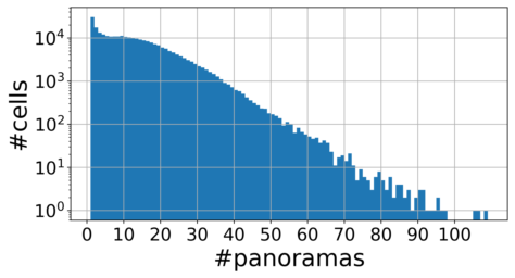
Figure 6: Histogram showing how many cells contain a given number of panorama. We can see that cells with only one panorama (which are discarded at train time as explained in Sec. B.2) are the most common. Note that the y axis is in logarithmic scale. The side of each cell (i.e. the hyperparameter $M$) is $M=10$ meters, as in our final experiments.

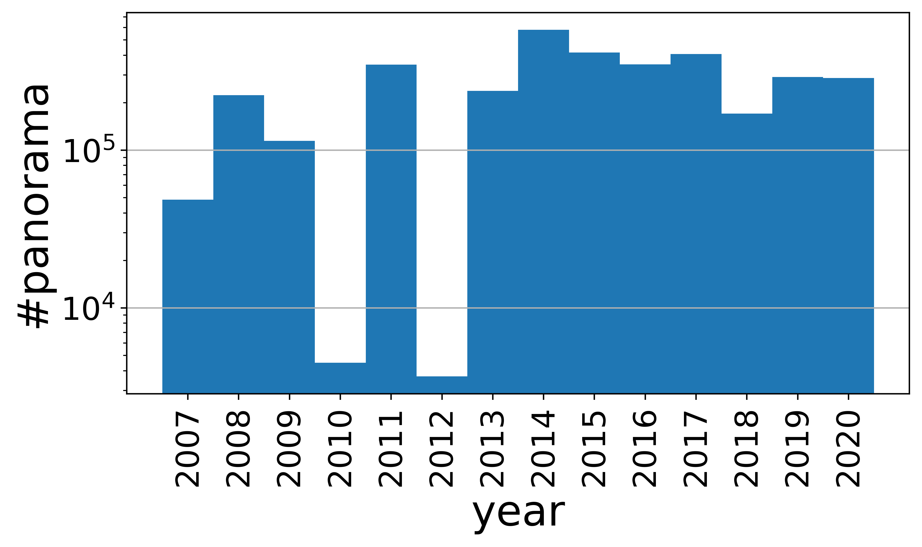
Figure 7: Number of 360°panorama of SF-XL for each given year.

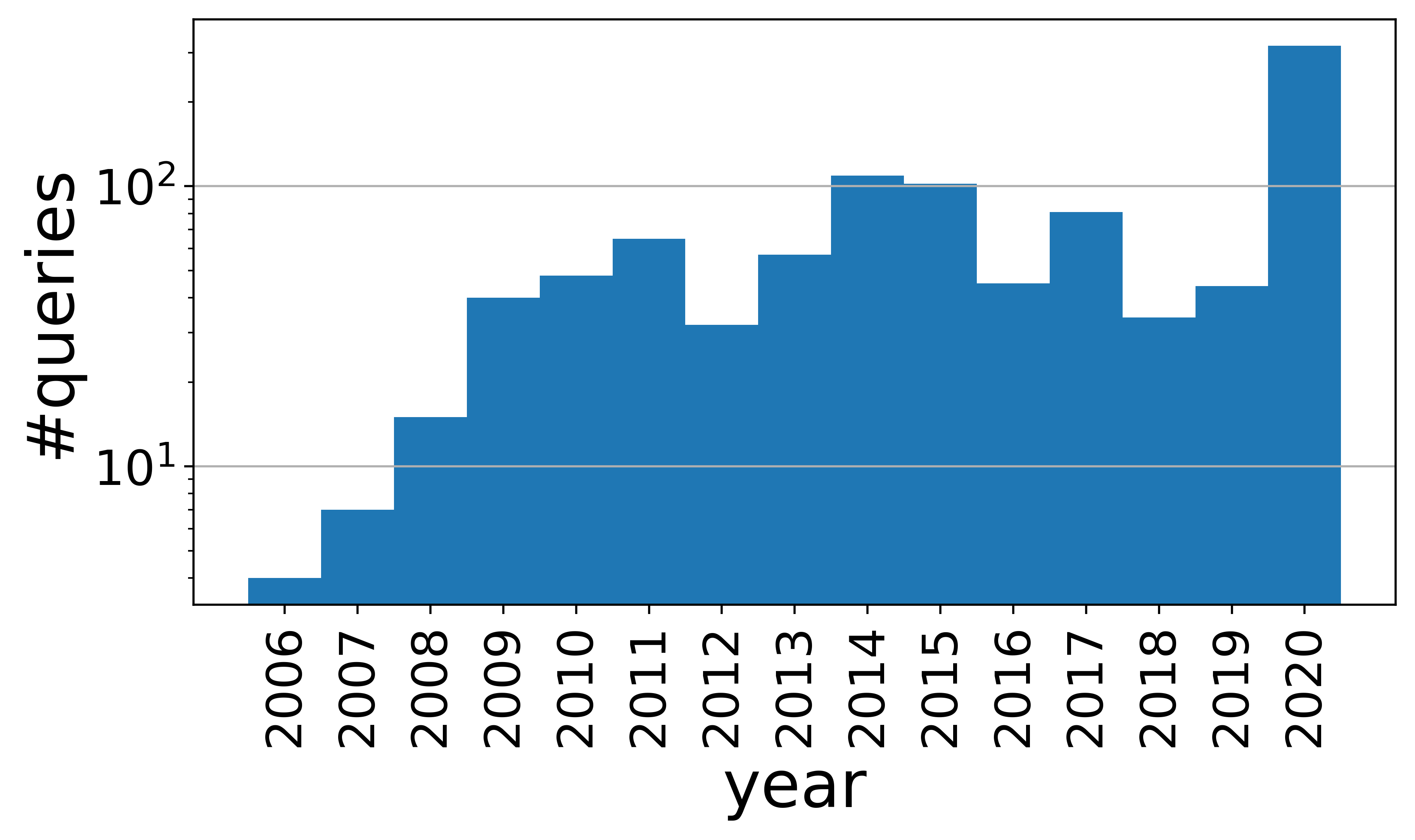
Figure 8: Number of queries from SF-XL test v1 for each given year.

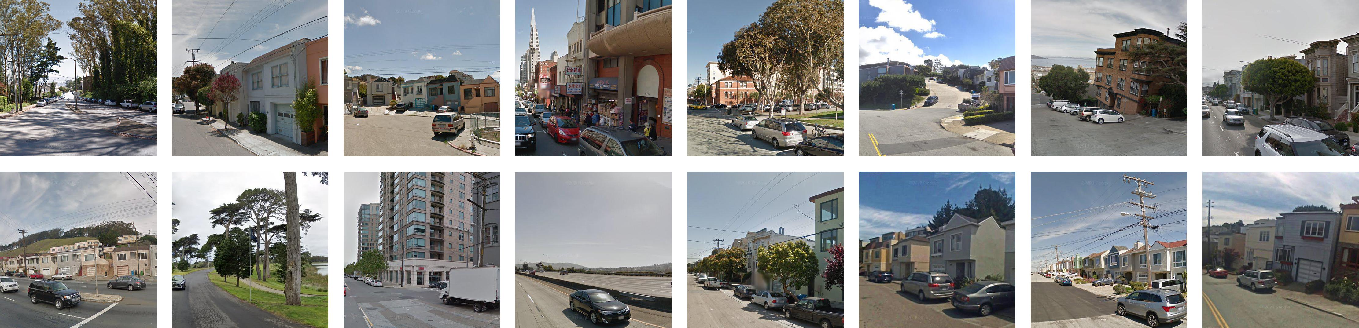
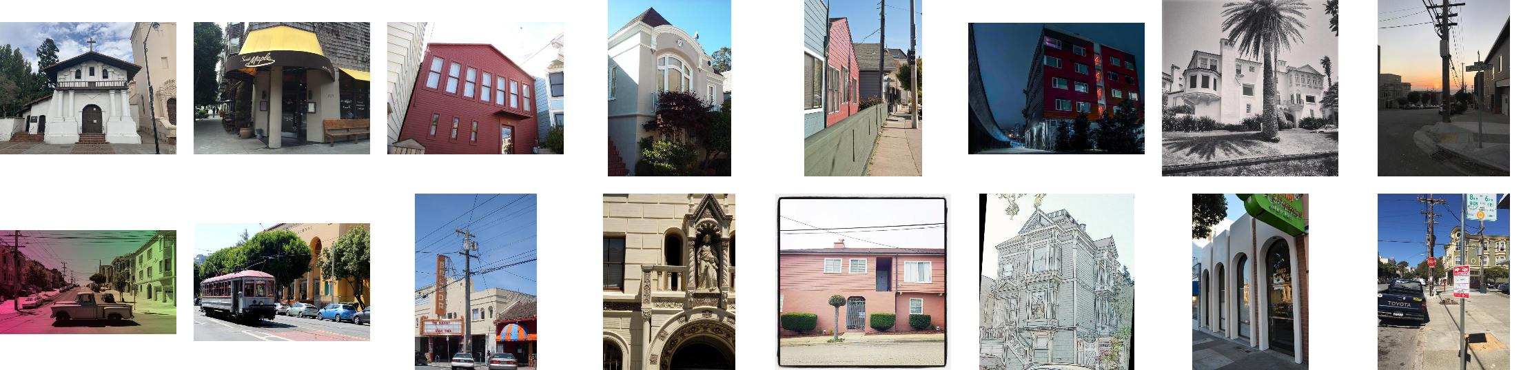
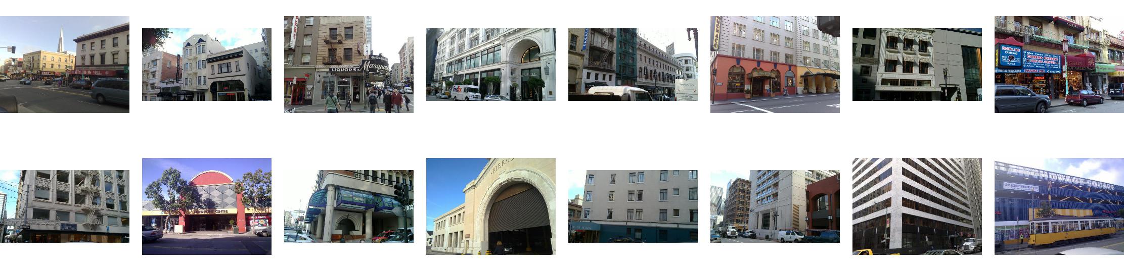
Figure 9: Examples from SF-XL. The first two rows of images are from the train set, the next two from the queries of SF-XL test v1, and the last two rows from the queries of SF-XL test v2.

   

   

Appendix B Experiments

B.1 Further ablations

In this section, we provide further results obtained by changing the hyperparameters of CosPlace to better understand their correlations to the final results.

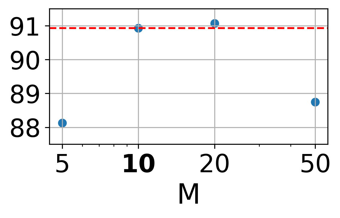
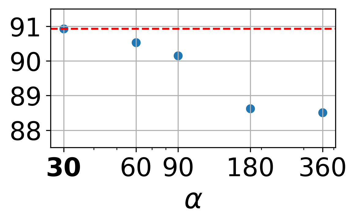
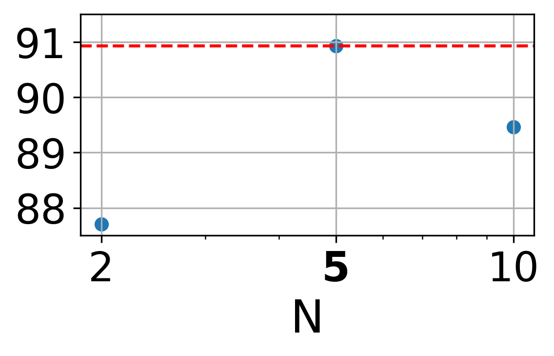
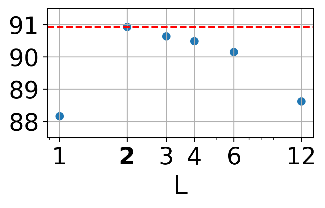
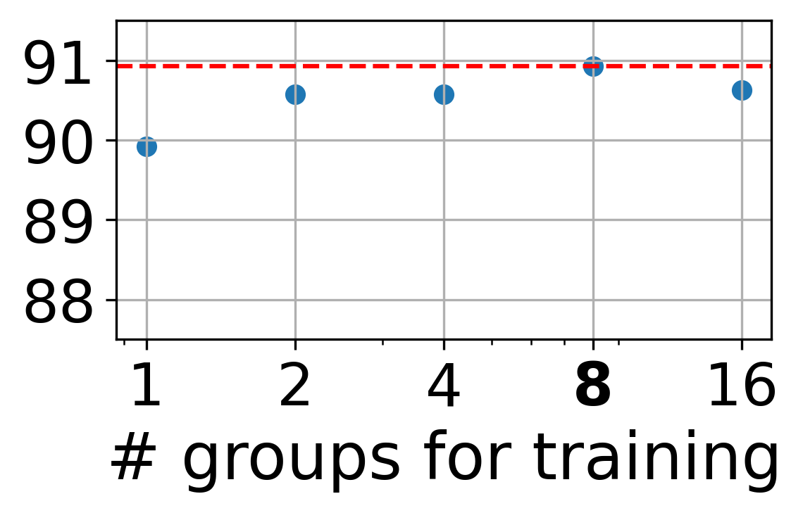
Figure 10: Full ablation on each hyperparameter. On the x axis are values for the hyperparameters, and on the y axis their respective recall@1 on the SF-XL val set, computed with a ResNet-18. Values in bold are the chosen ones for all experiments besides ablations, and the red line represents their recall@1.

In Fig. 10 we report an extensive ablation obtained by changing the parameters used to split the dataset into groups and classes, namely $M$, $\alpha$, $N$ and $L$, as well as using a different number of groups for training. Among other results, we see in the rightmost plot that using just a single group for training the model leads to a drop in recall@1 of just 1%, and that the optimal results are achieved using 8 of the 50 groups.

To better understand the importance that the GeM pooling [40] has within the architecture used for CosPlace, we provide a set of experiments by replacing it with the average or max pooling in Tab. 7. From the table, we can see that CosPlace would outperform the previous state-of-the-art even with a standard architecture used for classification, made of a CNN backbone, a max pooling, and a fully connected layer.

Pooling Pitts250k Pitts30k Tokyo 24/7 MSLS St Lucia Average 88.5 87.6 73.7 78.5 98.7 Max 90.8 89.3 78.1 80.5 98.7 GeM 90.4 89.5 81.6 81.8 98.8

Table 7: Ablation over different pooling layers. This table shows results obtained by replacing the GeM layer with a max or average pooling. Results refer to the recall@1 obtained with a ResNet-18.

B.2 Further implementation details

Regarding CosPlace training, to ensure that each class is well represented, only cells with at least 10 panoramas are considered for training, effectively discarding about 15% of the images. The hyperparameters of $M=10$, $\alpha=30$, $N=5$, and $L=2$ lead to the creation of 50 groups, where each group ends up with roughly 35k classes, and each class contains on average 19.8 images. As explained in the main paper, we only train on 8 (out of 50) groups, which together contain roughly 5.6M images. Note that the total size of the SF-XL training set is 41.2M (i.e., we only use 13.6% of the images), meaning that train-time scalability is a factor that can still be vastly improved in future works.

We use the Adam optimizer [28] with a learning rate of 0.00001, and a batch size of 32 images. We use color jittering as in [18]. For results to be fair with [18], which uses a smart region cropping method, we also employ random cropping. Finally, the margin of the cosFace loss is set to 0.40.

Number of hyperparameters. Although CosPlace introduces a considerable amount of hyperparameters, we also note that there is no more need for many other ones used in previous state-of-the-art methods [1, 32, 18], such as the number of negatives per query (usually set to 10), refresh rate of the cache (1000), pool size of randomly sampled negatives (1000), threshold distance for train-time potential positives (10 meters) and the number of cluster in NetVLAD layer (64). Moreover, the intuitive meaning of the hyperparameters in CosPlace in comparison to the less obvious mining hyperparameters makes it easier to set them using common sense: for example, it is clear that a small $M$ (or $\alpha$) leads to little intra-class spatial variations, while a large $M$ (or $\alpha$) may cause two images of the same class to be too different; similarly, using a small value for $N$ leads to a higher similarity between inter-class (but same group) images, while using a very high $N$ leads to classes being very geographically spread out, which can be a problem with smaller datasets (because groups would have few classes).

B.3 Exploratory experiments

B.3.1 Further results on backbones and descriptors dimensionality.

Given that previous methods (as recent as 2021) in Visual geo-localization rely on relatively old VGG-16 [43] or AlexNet [31] backbones [1, 27, 32, 18, 57, 36, 37], we believe that this is widening an already large gap between research and real-world applications, where one would want to obtain the best possible results with the lowest computational complexity. To narrow such a gap, we investigate how the use of more recent backbones can enhance CosPlace and lead to better results, smaller descriptors, and faster computation. To this end, we train CosPlace using a number of backbones, namely VGG-16 [43], ResNet-18, ResNet-50, ResNet-101 [23], ViT [16], CCT224 and CCT384 [20]. All CNN backbones (i.e., VGG-16 and ResNets) are followed by a GeM pooling [40] and a fully connected layer, Moreover, we experiment with various powers of 2 (from 32-D to 2048-D) as output dimension. Regarding transformers-based neural networks, we use the 384-D SeqPool output of CCT as descriptors, and for ViT, we obtain the 768-D output by feeding the CLS token to a multi-layer perceptron with tanh, following its original implementation [16]. Preliminary results showed that directly using ViT’s CLS token led to lower recalls.

Results from Fig. 11 clearly show that CosPlace presents encouraging results regardless of the depth of the backbone, and we argue that future works should focus on more modern architectures, such as the ResNets, which are generally faster, lighter and achieve comparable or better results than the commonly used VGG-16. We also see that CosPlace is able to reach remarkable recalls and robustness with very low dimensions; for example, we see that any 128-D architecture trained with CosPlace outperforms 4096-D NetVLAD (which is trained on Pitts30k) on any test dataset.

While transformers achieve lower results, we want to point out that we used the same hyperparameters for all experiments (e.g., same learning rate and optimizer), and we believe that performing a proper hyperparameter tuning independently for each backbone can increase the results shown in Fig. 11, at the cost of a large number of experiments. Moreover, while we used a resolution of $512\times 512$ for CNNs, transformers require a smaller size, respectively $224\times 224$ for ViT and CCT224, and $384\times 384$ for CCT384, and this can provide a further explanation of the lower results with transformers.

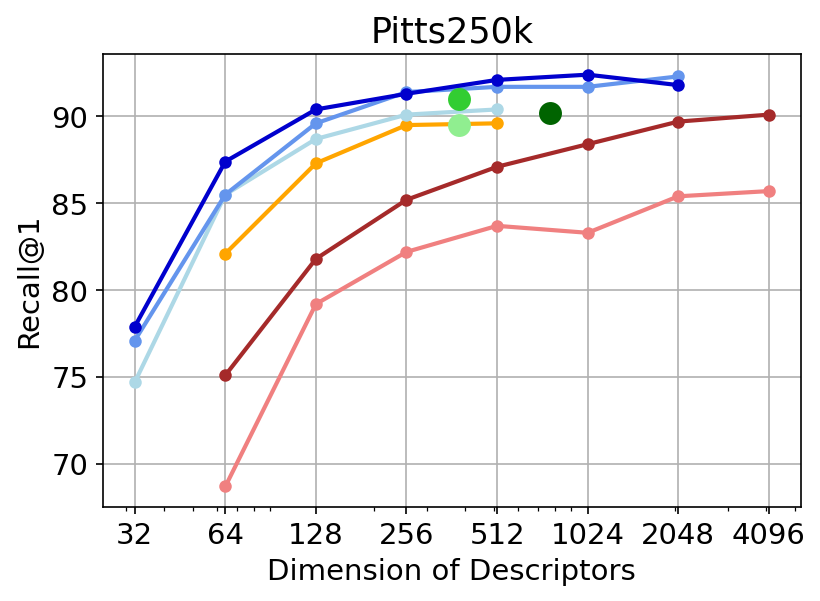
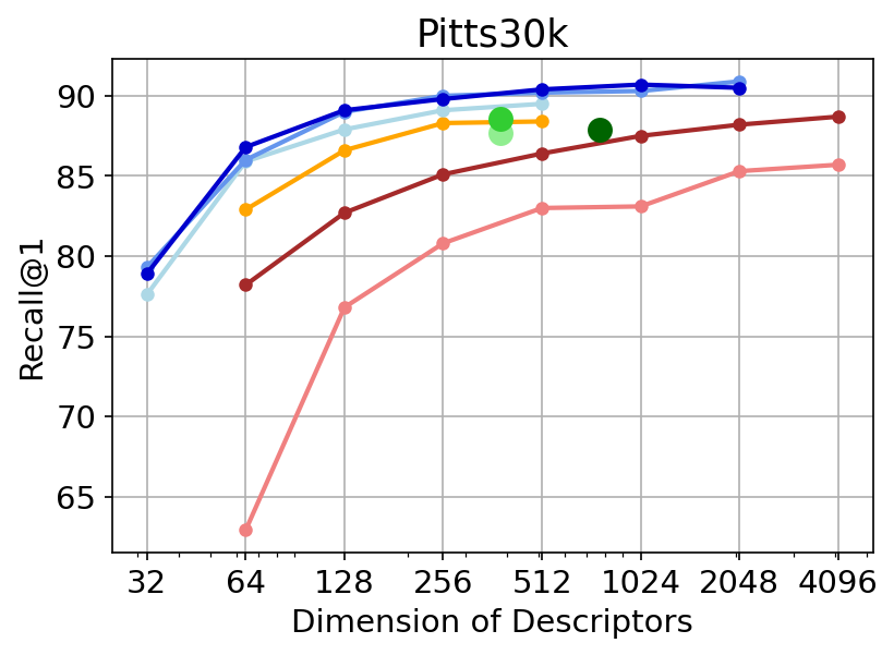
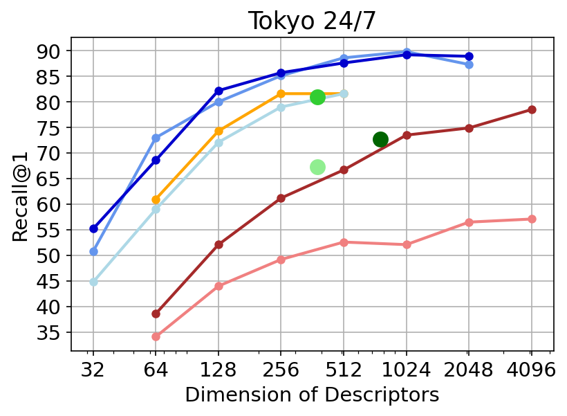
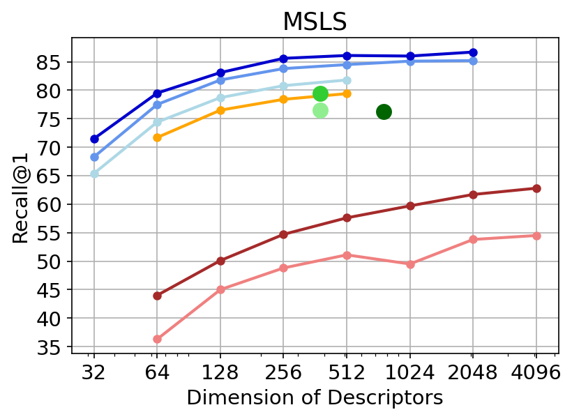
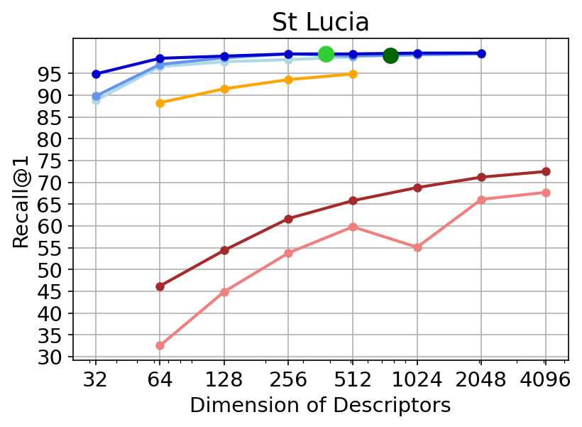
Figure 11: Further results on backbones and descriptors dimensionality. Results on a number of datasets of CosPlace using different backbones and dimensionalities, compared with SFRS and NetVLAD trained on Pitts30k.

Method Desc. dim. Train set Pitts250k Pitts30k Tokyo 24/7 MSLS St Lucia R@1 R@5 R@1 R@5 R@1 R@5 R@1 R@5 R@1 R@5 GeM [40] 512 Pitts30k 75.3$\pm$ 0.2 88.4$\pm$ 0.3 77.9$\pm$ 0.4 90.5$\pm$ 0.3 46.4$\pm$ 0.9 65.3$\pm$ 0.7 51.8$\pm$ 0.9 64.4$\pm$ 0.9 59.9$\pm$ 1.6 76.3$\pm$ 2.0 GeM [40] 512 MSLS 65.3$\pm$ 1.2 81.0$\pm$ 1.6 71.6$\pm$ 2.1 85.1$\pm$ 1.9 44.9$\pm$ 1.7 62.6$\pm$ 1.2 66.7$\pm$ 0.7 78.9$\pm$ 0.5 84.6$\pm$ 1.1 93.3$\pm$ 0.7 GeM [40] 512 SF-XL* 64.7$\pm$ 0.8 81.4$\pm$ 0.8 67.8$\pm$ 0.6 83.6$\pm$ 0.7 37.9$\pm$ 2.3 51.0$\pm$ 2.1 46.8$\pm$ 2.1 58.1$\pm$ 1.2 68.5$\pm$ 2.4 82.7$\pm$ 1.8 NetVLAD [1] 512 Pitts30k 83.7$\pm$ 0.3 92.8$\pm$ 0.1 83.0$\pm$ 0.2 92.6$\pm$ 0.3 52.6$\pm$ 1.1 70.9$\pm$ 1.2 51.1$\pm$ 1.0 63.5$\pm$ 0.8 59.8$\pm$ 0.5 74.5$\pm$ 1.2 NetVLAD [1] 512 MSLS 74.6$\pm$ 1.3 86.8$\pm$ 1.2 77.0$\pm$ 0.9 88.6$\pm$ 1.2 50.5$\pm$ 2.2 65.1$\pm$ 1.7 72.6$\pm$ 0.5 83.0$\pm$ 0.3 92.6$\pm$ 0.6 97.1$\pm$ 0.4 NetVLAD [1] 512 SF-XL* 77.5$\pm$ 0.5 88.5$\pm$ 0.2 79.7$\pm$ 0.3 90.0$\pm$ 0.4 53.0$\pm$ 0.9 70.2$\pm$ 0.5 53.1$\pm$ 3.2 64.2$\pm$ 2.2 78.7$\pm$ 1.6 88.1$\pm$ 1.8 CRN [27] 512 Pitts30k 84.6$\pm$ 0.6 93.6$\pm$ 0.3 84.3$\pm$ 0.2 92.7$\pm$ 0.2 53.4$\pm$ 0.5 70.6$\pm$ 0.8 54.1$\pm$ 0.6 66.1$\pm$ 0.6 56.6$\pm$ 2.7 75.5$\pm$ 2.9 APANet [57] † 512 Pitts30k 83.7 92.6 - - 67.0 81.0 - - - - SARE [32] 512 Pitts30k 84.3$\pm$ 0.7 92.6$\pm$ 0.4 84.7$\pm$ 0.7 92.6$\pm$ 0.5 62.0$\pm$ 0.6 74.9$\pm$ 0.4 55.8$\pm$ 3.3 67.8$\pm$ 3.3 63.4$\pm$ 3.0 79.0$\pm$ 1.9 SFRS [18] 512 Pitts30k 87.1$\pm$ 0.4 94.6$\pm$ 0.2 86.4$\pm$ 0.5 93.8$\pm$ 0.2 66.7$\pm$ 1.0 79.6$\pm$ 0.9 57.6$\pm$ 1.1 68.9$\pm$ 1.0 65.8$\pm$ 3.1 80.1$\pm$ 2.3 SRALNet [36] † 512 Pitts30k 84.8 93.5 - - 60.6 76.5 - - - - APPSVR [37] † 512 Pitts30k 85.3 94.0 - - 62.0 76.5 - - - - CosPlace (Ours) 512 SF-XL 89.3$\pm$ 0.2 96.2$\pm$ 0.3 88.5$\pm$ 0.1 94.5$\pm$ 0.2 82.2$\pm$ 0.5 88.9$\pm$ 0.9 79.6$\pm$ 0.5 87.2$\pm$ 0.4 94.1$\pm$ 0.8 97.4$\pm$ 0.1

Table 8: Comparisons of various methods on popular datasets with 512-D descriptors. This table is the equivalent of Tab. 3 in the main paper, but here all descriptors have the same dimensionality.

Method Desc. dim. Train set SF-XL test v1 SF-XL test v2 R@1 R@5 R@10 R@1 R@5 R@10 GeM 512 Pitts30k 21.7 30.3 34.4 43.1 63.7 69.2 GeM 512 MSLS 8.1 15.6 20.2 29.3 46.3 53.8 GeM 512 SF-XL* 9.8 17.6 21.2 34.8 55.5 63.0 NetVLAD 512 Pitts30k 27.4 38.1 43.6 66.7 79.3 82.9 NetVLAD 512 MSLS 14.5 21.0 28.9 40.5 59.7 64.4 NetVLAD 512 SF-XL* 25.4 32.9 40.5 66.9 78.6 82.8 CRN 512 Pitts30k 31.4 43.0 49.7 68.2 81.3 83.3 SARE 512 Pitts30k 30.8 42.1 46.5 69.2 81.1 83.1 SFRS 512 Pitts30k 35.6 49.7 54.8 78.1 88.5 91.3 CosPlace (Ours) 512 SF-XL 65.1 73.6 77.6 83.4 92.1 94.8

Table 9: Comparisons of various methods on SF-XL test v1 and SF-XL test v2 with 512-D descriptors. This table is the equivalent of Tab. 4 in the main paper.

B.3.2 Comparison with other methods using same descriptors dimensionality.

Given that CosPlace uses much lower dimensionality of descriptors, in Tab. 8 and Tab. 9 we report the equivalent experiments of Tab. 3 and Tab. 4 of the main paper, but using the same (512) dimensionality for all methods. We can see that in this scenario, the advantages of CosPlace w.r.t. previous works are even more noticeable.

B.3.3 Comparison with models trained on Google Landmark.

In Tab. 10, we compare models trained using CosPlace on SF-XL with models trained on two popular landmark retrieval (LR) datasets, namely the Google Landmark (GLD) and SfM120k [40]. Models trained on GLD and SfM120k are downloaded from the official repository of [40] , which relied on a triplet loss for training. CosPlace can’t be used on such landmark retrieval datasets, as they lack GPS coordinates and heading labels.

Note that these experiments are not aimed at providing a rigorous comparison of CosPlace vs triplet losses or SF-XL vs standard retrieval datasets, given that the underlying tasks (i.e. VG and LR) present many differences; we just want to provide an intuition on how popular models trained for LR fare on VG datasets.

Training Dataset	Backbone	Pitts250k	Pitts30k	Tokyo 24/7	MSLS	St Lucia
SfM120k	ResNet-50	84.5	83.4	75.2	64.5	73.9
GLD	ResNet-50	85.8	84.1	77.8	69.5	77.3
SF-XL	ResNet-50	92.3	90.9	87.3	85.2	99.5
SfM120k	ResNet-101	85.0	83.9	77.5	64.7	76.3
GLD	ResNet-101	86.9	85.1	77.8	72.4	83.4
SF-XL	ResNet-101	91.8	90.5	88.9	86.7	99.7

Table 10: Comparison with models trained on large landmark retrieval datasets. The models trained on SF-XL is trained with CosPlace, while models trained on GLD and SfM120k rely on a triplet loss. All models are equivalent (i.e. ResNets followed by a GeM pooling and a fully connected layer with output dimensionality 512).

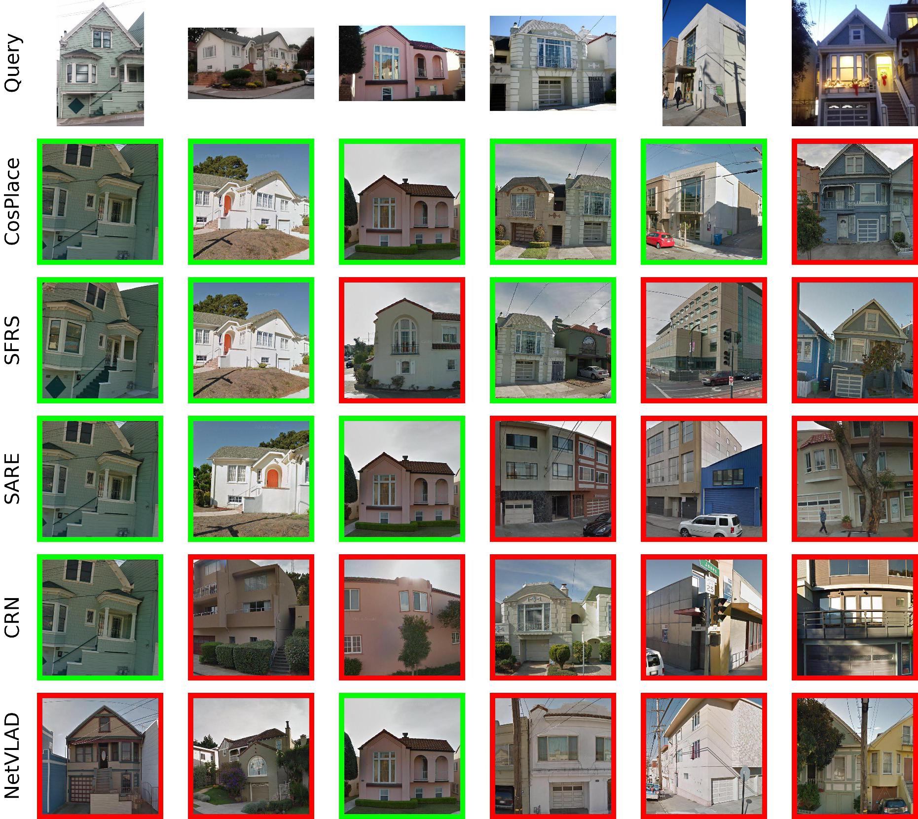
Figure 12: Qualitative comparisons of retrieved images for a number of methods.

B.3.4 Comparison with other methods: qualitative results.

Figure 12 shows some qualitative results of retrieved images with CosPlace compared to previous SOTA methods such as NetVLAD [1], CRN [27], SARE [32] and SFRS [18].

References

- [1] Relja Arandjelović, Petr Gronat, Akihiko Torii, Tomas Pajdla, and Josef Sivic. NetVLAD: CNN architecture for weakly supervised place recognition. IEEE Transactions on Pattern Analysis and Machine Intelligence, 40(6):1437–1451, 2018.
- [2] Aayush Bansal, Hernán Badino, and Daniel F. Huber. Understanding how camera configuration and environmental conditions affect appearance-based localization. In 2014 IEEE Intelligent Vehicles Symposium Proceedings, Dearborn, MI, USA, June 8-11, 2014, pages 800–807. IEEE, 2014.
- [3] Gabriele Berton, Carlo Masone, Valerio Paolicelli, and Barbara Caputo. Viewpoint invariant dense matching for visual geolocalization. In IEEE International Conference on Computer Vision, pages 12169–12178, October 2021.
- [4] Gabriele Berton, Riccardo Mereu, Gabriele Trivigno, Carlo Masone, Gabriela Csurka, Torsten Sattler, and Barbara Caputo. Deep visual geo-localization benchmark. In Proceedings of the IEEE Conference on Computer Vision and Pattern Recognition, 2022.
- [5] Gabriele Berton, Valerio Paolicelli, Carlo Masone, and Barbara Caputo. Adaptive-attentive geolocalization from few queries: A hybrid approach. In IEEE Winter Conference on Applications of Computer Vision, pages 2918–2927, January 2021.
- [6] B. Cao, A. Araujo, and J. Sim. Unifying deep local and global features for image search. In European Conference on Computer Vision, pages 726–743. Springer Int. Publishing, 2020.
- [7] N. Carlevaris-Bianco, A. K. Ushani, and R. M. Eustice. University of Michigan North Campus long-term vision and lidar dataset. The International Journal of Robotics Research, 35(9):1023–1035, 2016.
- [8] D. M. Chen, G. Baatz, K. Köser, S. S. Tsai, R. Vedantham, T. Pylvänäinen, K. Roimela, X. Chen, J. Bach, M. Pollefeys, B. Girod, and R. Grzeszczuk. City-scale landmark identification on mobile devices. In IEEE Conference on Computer Vision and Pattern Recognition, pages 737–744, 2011.
- [9] Z. Chen, A. Jacobson, N. Sünderhauf, B. Upcroft, L. Liu, C. Shen, I. Reid, and M. Milford. Deep learning features at scale for visual place recognition. In 2017 IEEE International Conference on Robotics and Automation, pages 3223–3230, 2017.
- [10] Z. Chen, L. Liu, I. Sa, Z. Ge, and M. Chli. Learning context flexible attention model for long-term visual place recognition. IEEE Robotics and Automation Letters, 3(4):4015–4022, 2018.
- [11] Z. Chen, F. Maffra, I. Sa, and M. Chli. Only look once, mining distinctive landmarks from ConvNet for visual place recognition. In 2017 IEEE/RSJ International Conference on Intelligent Robots and Systems, pages 9–16, 2017.
- [12] R. Cheng, K. Wang, J. Bai, and Z. Xu. Unifying visual localization and scene recognition for people with visual impairment. IEEE Access, 8:64284–64296, 2020.
- [13] M. Cummins and P. Newman. Highly scalable appearance-only slam - FAB-MAP 2.0. In Robotics: Science and Systems, 2009.
- [14] Jiankang Deng, J. Guo, and S. Zafeiriou. ArcFace: Additive angular margin loss for deep face recognition. In IEEE Conference on Computer Vision and Pattern Recognition, pages 4685–4694, 2019.
- [15] A.-D. Doan, Y. Latif, T.-J. Chin, Y. Liu, T.-T. Do, and I. Reid. Scalable place recognition under appearance change for autonomous driving. In IEEE International Conference on Computer Vision, pages 9319–9328, October 2019.
- [16] Alexey Dosovitskiy, Lucas Beyer, Alexander Kolesnikov, Dirk Weissenborn, Xiaohua Zhai, Thomas Unterthiner, Mostafa Dehghani, Matthias Minderer, Georg Heigold, Sylvain Gelly, Jakob Uszkoreit, and Neil Houlsby. An Image is Worth 16x16 Words: Transformers for Image Recognition at Scale. ArXiv, abs/2010.11929, 2021.
- [17] S. Garg, N. Suenderhauf, and M. Milford. Semantic–geometric visual place recognition: a new perspective for reconciling opposing views. The International Journal of Robotics Research, 2019.
- [18] Yixiao Ge, Haibo Wang, Feng Zhu, Rui Zhao, and Hongsheng Li. Self-supervising fine-grained region similarities for large-scale image localization. In Andrea Vedaldi, Horst Bischof, Thomas Brox, and Jan-Michael Frahm, editors, Computer Vision – ECCV 2020, pages 369–386, Cham, 2020. Springer International Publishing.
- [19] A Geiger, P Lenz, C Stiller, and R Urtasun. Vision meets robotics: The KITTI dataset. The International Journal of Robotics Research, 32(11):1231–1237, 2013.
- [20] Ali Hassani, Steven Walton, Nikhil Shah, Abulikemu Abuduweili, Jiachen Li, and Humphrey Shi. Escaping the Big Data Paradigm with Compact Transformers. ArXiv, abs/2104.05704, 2021.
- [21] Stephen Hausler, Sourav Garg, Ming Xu, Michael Milford, and Tobias Fischer. Patch-netvlad: Multi-scale fusion of locally-global descriptors for place recognition. In IEEE Conference on Computer Vision and Pattern Recognition, pages 14141–14152, 2021.
- [22] S. Hausler, A. Jacobson, and M. Milford. Multi-process fusion: Visual place recognition using multiple image processing methods. IEEE Robotics and Automation Letters, 4(2):1924–1931, 2019.
- [23] K. He, X. Zhang, S. Ren, and J. Sun. Deep residual learning for image recognition. In IEEE Conference on Computer Vision and Pattern Recognition, pages 770–778, 2016.
- [24] Sarah Ibrahimi, Nanne van Noord, Tim Alpherts, and Marcel Worring. Inside out visual place recognition. In British Machine Vision Conference, 2021.
- [25] Mike Izbicki, Evangelos Papalexakis, and Vassilis Tsotras. Exploiting the earth’s spherical geometry to geolocate images. In Ulf Brefeld, Élisa Fromont, Andreas Hotho, Arno J. Knobbe, Marloes H. Maathuis, and Céline Robardet, editors, Machine Learning and Knowledge Discovery in Databases - European Conference, ECML PKDD 2019, Würzburg, Germany, September 16-20, 2019, Proceedings, Part II, volume 11907 of Lecture Notes in Computer Science, pages 3–19. Springer, 2019.
- [26] A. Khaliq, S. Ehsan, Z. Chen, M. Milford, and K. McDonald-Maier. A holistic visual place recognition approach using lightweight CNNs for significant viewpoint and appearance changes. IEEE Transactions on Robotics, 36(2):561–569, 2020.
- [27] Hyo Jin Kim, Enrique Dunn, and Jan-Michael Frahm. Learned contextual feature reweighting for image geo-localization. In IEEE Conference on Computer Vision and Pattern Recognition, pages 3251–3260, 2017.
- [28] Diederik Kingma and Jimmy Ba. Adam: A method for stochastic optimization. International Conference on Learning Representations, 12 2014.
- [29] J. Knopp, J. Sivic, and T. Pajdla. Avoiding confusing features in place recognition. In Proceedings of the European Conference on Computer Vision, 2010.
- [30] Giorgos Kordopatis-Zilos, Panagiotis Galopoulos, S. Papadopoulos, and Y. Kompatsiaris. Leveraging efficientnet and contrastive learning for accurate global-scale location estimation. ACM International Conference on Multimedia Retrieval, 2021.
- [31] A. Krizhevsky, I. Sutskever, and G. E. Hinton. ImageNet classification with deep convolutional neural networks. In F. Pereira, C. J. C. Burges, L. Bottou, and K. Q. Weinberger, editors, Advances in Neural Information Processing Systems 25, pages 1097–1105. Curran Associates, Inc., 2012.
- [32] Liu Liu, Hongdong Li, and Yuchao Dai. Stochastic Attraction-Repulsion Embedding for Large Scale Image Localization. In IEEE International Conference on Computer Vision, 2019.
- [33] W. Maddern, G. Pascoe, C. Linegar, and P. Newman. 1 Year, 1000km: The Oxford RobotCar Dataset. The International Journal of Robotics Research, 2017.
- [34] Michael Milford and G. Wyeth. Mapping a suburb with a single camera using a biologically inspired slam system. IEEE Transactions on Robotics, 24:1038–1053, 2008.
- [35] Eric Müller-Budack, Kader Pustu-Iren, and Ralph Ewerth. Geolocation estimation of photos using a hierarchical model and scene classification. In Computer Vision - ECCV 2018 - 15th European Conference, Munich, Germany, September 8-14, 2018, Proceedings, Part XII, volume 11216 of Lecture Notes in Computer Science, pages 575–592. Springer, 2018.
- [36] Guohao Peng, Yufeng Yue, Jun Zhang, Zhenyu Wu, Xiaoyu Tang, and Danwei Wang. Semantic reinforced attention learning for visual place recognition. In IEEE International Conference on Robotics and Automation, pages 13415–13422. IEEE, 2021.
- [37] Guohao Peng, Jun Zhang, Heshan Li, and Danwei Wang. Attentional pyramid pooling of salient visual residuals for place recognition. In IEEE International Conference on Computer Vision, pages 885–894, October 2021.
- [38] James Philbin, Ondrej Chum, Michael Isard, Josef Sivic, and Andrew Zisserman. Object retrieval with large vocabularies and fast spatial matching. In IEEE Conference on Computer Vision and Pattern Recognition. IEEE Computer Society, 2007.
- [39] James Philbin, Ondrej Chum, Michael Isard, Josef Sivic, and Andrew Zisserman. Lost in quantization: Improving particular object retrieval in large scale image databases. In IEEE Conference on Computer Vision and Pattern Recognition, June 2008.
- [40] F. Radenović, G. Tolias, and O. Chum. Fine-tuning CNN Image Retrieval with No Human Annotation. IEEE Transactions on Pattern Analysis and Machine Intelligence, 2018.
- [41] Torsten Sattler, Tobias Weyand, Bastian Leibe, and Leif Kobbelt. Image retrieval for image-based localization revisited. In IEEE Conference on Computer Vision and Pattern Recognition, 2012.
- [42] Paul Hongsuck Seo, Tobias Weyand, Jack Sim, and Bohyung Han. Cplanet: Enhancing image geolocalization by combinatorial partitioning of maps. In ECCV, 2018.
- [43] Karen Simonyan and Andrew Zisserman. Very deep convolutional networks for large-scale image recognition. In International Conference on Learning Representations, 2015.
- [44] Yash Srivastava, Vaishnav Murali, and Shiv Ram Dubey. A performance comparison of loss functions for deep face recognition, 2019.
- [45] Fuwen Tan, Jiangbo Yuan, and Vicente Ordonez. Instance-level image retrieval using reranking transformers. In IEEE International Conference on Computer Vision, 2021.
- [46] A. Torii, R. Arandjelović, J. Sivic, M. Okutomi, and T. Pajdla. 24/7 place recognition by view synthesis. IEEE Transactions on Pattern Analysis and Machine Intelligence, 40(2):257–271, 2018.
- [47] A. Torii, J. Sivic, M. Okutomi, and T. Pajdla. Visual place recognition with repetitive structures. IEEE Transactions on Pattern Analysis and Machine Intelligence, 37(11):2346–2359, 2015.
- [48] A. Torii, Hajime Taira, Josef Sivic, M. Pollefeys, M. Okutomi, T. Pajdla, and Torsten Sattler. Are large-scale 3d models really necessary for accurate visual localization? IEEE Transactions on Pattern Analysis and Machine Intelligence, 43:814–829, 2021.
- [49] Hao Wang, Yitong Wang, Zheng Zhou, Xing Ji, Dihong Gong, Jingchao Zhou, Zhifeng Li, and Wei Liu. Cosface: Large margin cosine loss for deep face recognition. In IEEE Conference on Computer Vision and Pattern Recognition, pages 5265–5274. Computer Vision Foundation / IEEE Computer Society, 2018.
- [50] Frederik Warburg, Soren Hauberg, Manuel Lopez-Antequera, Pau Gargallo, Yubin Kuang, and Javier Civera. Mapillary street-level sequences: A dataset for lifelong place recognition. In IEEE Conference on Computer Vision and Pattern Recognition, June 2020.
- [51] Tobias Weyand, A. Araújo, Bingyi Cao, and Jack Sim. Google landmarks dataset v2 – a large-scale benchmark for instance-level recognition and retrieval. In IEEE Conference on Computer Vision and Pattern Recognition, pages 2572–2581, 2020.
- [52] Tobias Weyand, Ilya Kostrikov, and James Philbin. Planet - photo geolocation with convolutional neural networks. In European Conference on Computer Vision, 2016.
- [53] Jun Yu, Chaoyang Zhu, Jian Zhang, Qingming Huang, and Dacheng Tao. Spatial pyramid-enhanced netvlad with weighted triplet loss for place recognition. IEEE Transactions on Neural Networks and Learning Systems, 31(2):661–674, 2020.
- [54] Mubariz Zaffar, Sourav Garg, Michael Milford, Julian Kooij, David Flynn, Klaus McDonald-Maier, and Shoaib Ehsan. VPR-Bench: An open-source visual place recognition evaluation framework with quantifiable viewpoint and appearance change. International Journal of Computer Vision, 129(7):2136–2174, 2021.
- [55] A.R. Zamir and M. Shah. Image geo-localization based on multiple nearest neighbor feature matching using generalized graphs. IEEE Transactions on Pattern Analysis and Machine Intelligence, PP(99):1–1, 2014.
- [56] Eyasu Zemene, Yonatan Tariku, Haroon Idrees, Andrea Prati, Marcello Pelillo, and Mubarak Shah. Large-scale image geo-localization using dominant sets. CoRR, abs/1702.01238, 2017.
- [57] Yingying Zhu, Jiong Wang, Lingxi Xie, and Liang Zheng. Attention-based pyramid aggregation network for visual place recognition. In 2018 ACM Multimedia Conference on Multimedia Conference, MM 2018, Seoul, Republic of Korea, October 22-26, 2018, pages 99–107. ACM, 2018.