Variable mass accretion and failed wind explain changing look phenomena in NGC 1365

Changing look active galactic nuclei (CLAGNs) show complex nature in their X-ray spectral shape and line of sight column density variation. The physical mechanisms responsible for these variations are unclear. Here, we study the spectral properties of a CLAGN, NGC 1365 using combined XMM-Newton and NuSTAR observations to understand the CL behavior. The model fitted mass accretion rate varied between $0.003\pm 0.001$ and $0.009\pm 0.002$ $\dot{M}_{\rm Edd}$ and the dynamic corona changed from $28\pm 3$ to $10\pm 1$ $r_{g}$. We found that the variable absorption column density correlates with the mass accretion rate and the geometry of the corona. The derived wind velocity was sufficiently low compared to the escape velocity to drive the wind away from the disc for the epochs when column densities were high. This suggests that the high and variable absorption can be due to failed winds from the disc. Our estimated ratio of mass outflow to inflow rate from the inner region of the disc lies between $0.019\pm 0.006$ and $0.12\pm 0.04$. From spectral fitting of the combined data, we found the mass of the central black hole to be constant $4.38\pm 0.34-4.51\pm 0.29\times 10^{6}M_{\odot}$, consistent with earlier findings. The confidence contours of $N_{H}$ with other model parameters show that the model fitted parameters are robust and non-degenerate. Our study construed that the changing accretion rate, which is a fundamental physical quantity and the geometry of the corona driving the CL phenomena in NGC 1365. The physical picture considered in this work connects both variable continuum and variable absorbing medium scenarios.

1 Introduction

An active galactic nucleus (AGN) is powered by the matter accreting onto the central supermassive black hole (SMBH) at the center of a galaxy. The radiation coming from the accreting AGN systems shows complex features in their X-ray spectra. The components (e.g. hard, soft, or soft excess etc.) of the spectra come from different regions within the system. Some fraction of the hard radiation heats up the disc and generates emission lines, while some fraction gets absorbed by different clouds at the line of sight (LOS). The variable absorption of the continuum coming from the central inner disc can be due to the presence of variable clouds or due to the winds from the disc.

The X-ray absorbing column density changes dramatically by an order of magnitude over a few years in different Seyfert galaxies (Risaliti et al., 2002), which disfavors the homogeneous nature of the absorbers. Changing look (CL) AGN are those sources that show extreme variation in the column density of the X-ray absorber, with rapid transitions between Compton-thin (N${}_{H}<10^{24}$ cm^-2) and Compton-thick (N${}_{H}>10^{24}$ cm^-2) regimes (e.g. Ricci et al., 2016). CLAGN though first discovered serendipitously (LaMassa et al., 2015) are now considered as a separate class of AGN that transit from type 1 to 2 and vice versa within a timescale of decades or years (Veron et al., 1980; Maiolino & Rieke, 1995a; Denney et al., 2014; Yang et al., 2018; Kim et al., 2018). In Ricci et al. (2020), the CL phenomena was shown for 1ES 1927+654 can be due to rapid changes in the innermost regions of accreting SMBHs.

According to models, the timescale of CL phenomenon within months or years can be due to the variation in absorbing material that appears and disappears along the LOS, this supports the quick variation in column density (Risaliti et al., 2009). On the contrary, many CLAGNs showed little variation in column density (McElroy et al., 2016; Noda & Done, 2018), therefore CL nature could also be due to other physical processes within the system. The weak or low optical polarization of CLAGNs suggests that the transition from type 1 to type 2 can not be attributed to the putative dust obscuration (e.g. Hutsemékers et al., 2019). The mid-infrared and optical analysis of Sheng et al. (2017) do not favor the obscuration scenario and support that the CL may be caused by the intrinsic variation of accretion process. The work of Noda & Done (2018) suggests CL as accretion process originated phenomenon where radiation pressure should be more important compared to gas pressure. The radiation pressure driven instability is also a possibility to explain the observed timescale of CL phenomenon (Śniegowska & Czerny, 2019).

NGC 1365 is a Seyfert 1.8 (Maiolino & Rieke, 1995b) galaxy at z=0.0055 with a $10^{6.5}M_{\odot}$ BH (Risaliti et al., 2009). Combes et al. (2019) estimated the mass of $3.98\times 10^{6}M_{\odot}$ from the molecular gas dynamics using ALMA data. This spiral galaxy is intensely studied by Lindblad (1999, for a review). The source is a CLAGN due to its Compton-thin to Compton-thick transition, that can be due to variation in the LOS absorber rather than to extreme intrinsic emission variability (Matt et al., 2003; Risaliti et al., 2005). The spectral components of NGC 1365 in X-ray consists of several distinct features e.g. Compton hump $>10$ keV, soft excess at low energy (below 3 keV), strong absorption features, relativistic iron and emission lines. The source also has bi-conical outflow from the nucleus (Edmunds et al., 1988). Sandqvist et al. (1995) suggested that the AGN has a weak radio jet in this source. A [O III] line is seen in the outflow (Storchi-Bergmann & Bonatto, 1991; Veilleux et al., 2003; Sharp & Bland-Hawthorn, 2010). The emission lines observed for this source are dominated by collisionally ionized gas (Guainazzi et al., 2009), however, it can also be hybrid (photoionised+collisionally ionised; Whewell et al., 2016, used XMM-Newton and Chandra data). NGC 1365 has some important characteristics, when it is observed in the Compton-thin state, its X-ray spectrum shows the presence of strong absorption lines due to Fe xxv(both the He-$\alpha$ and He-$\beta$) and Fexxvi(both the Ly$\alpha$ and Ly$\beta$ components); these lines are blue shifted by v$\sim$3000 km s^-1 (Risaliti et al., 2005; Brenneman et al., 2013). These features can be originated due to the presence of highly ionised outflowing wind and possibly originated from the accretion disc. All these features are occasionally observed in Seyfert galaxies, however, it is unlikely to see all of them in a single source. Later, Connolly et al. (2014) examined that the long-term variability of the X-ray absorber could be originated from the changes in mass accretion rate of NGC 1365. The analysis of Suzaku observation of the source suggested the presence of a partial covering and ionized absorber using photoionisation models (Gofford et al., 2013, 2015). Braito et al. (2014) evidenced that two ionised absorbers were needed to fit the RGS spectra of XMM-Newton and detected a possible P-Cygni profile of the Mg XII Ly$\alpha$ line which is associated with mildly ionized absorber indicative of a wide angle outflowing wind. At the same time, using the Chandra data, Nardini et al. (2015) estimated the location of the photoionised gas based on some evidence of broadening of the emission lines. The central active nucleus is surrounded by a molecular torus with both narrow and broad emission line components in the emitted spectrum and relativistic iron line (Risaliti et al., 2009). The variable absorbing medium along the LOS was observed by (Rivers et al., 2015) using combined XMM-Newton and NuSTAR data. The relativistic line feature estimates the maximal spin of the BH $>0.97$ (Walton et al., 2014). Kara et al. (2015) estimated soft lag due to the presence of eclipsing cloud along the line of sight using NuSTAR observations. The star formation and gas accretion to the central object were studied using near-infrared (NIR) data by Fazeli et al. (2019) and Gao et al. (2021) to check for more recent star formation activities and outflow structure of the source.

Despite the source has been studied extensively in different energy bands, the understanding of CL phenomena is still lacking due to shortcoming of physical picture in earlier studies. Most of them phenomenologically explained that the variable column density is due to the appearance/disappearance of some clouds along the LOS and none of the previous studies self-consistently considered the accretion-ejection scenario to take into account for the CL phenomena. Therefore, in this work, we aim to address that phenomena after estimating fundamental physical quantities of accretion e.g. mass accretion rate, corona geometry etc., considering the beforehand observational characteristics such as Compton hump, jets, winds, and variable continuum in NGC 1365 system. For that, we used joint XMM-Newton and NuSTAR data during 2012 and 2013. This paper is organized as follows: in Section 2 we explain the observations and data reduction procedures, in Section 3, we discuss the modelling, various analysis, and data fitting carried out using different models. A brief conclusion is given in the final Section.

2 Observation and Data analysis

We used joint XMM-Newton and NuSTAR (Harrison et al., 2013) observations of NGC 1365 during 2012 and 2013. The log of observations is given in Table 1.

Table 1: Log of observations. Here, X=6000204600, and Y=0692840 are the initials of the observation IDs.

NuSTAR	Exp.	XMM-Newton	Exp.	Epoch	Date	MJD
	(ks)		(ks)
X3	41	Y201	118	A	2012-07-26	56134
X5	66	Y301	108	B	2012-12-24	56285
X7	74	Y401	93	C	2013-01-23	56315
X9	70	Y501	116	D	2013-02-12	56335

To analyze the XMM-Newton data, we used the Science Analysis System (SAS) version 19.1.0 and followed the standard procedures given in the SAS data analysis threads. We first reprocessed the Observation Data Files (ODF) using the epproc routine to generate the calibrated and concatenated event lists. We filtered the concatenated event lists to remove the periods of high background activity. We then extracted the source and background spectra using the evselect routine. We used a circular region of radius $32^{\prime\prime}$ for both the source and the background. The background region was in the same CCD but away from the contamination of the point sources. We used rmfgen and arfgen tasks to generate the redistribution matrices (.rmf) and the ancillary (.arf) files. Finally, we rebinned the spectra using the task specgroup to have at least 25 counts in each bin.

The NuSTAR data were extracted using the standard NUSTARDAS v1.3.1 software. We ran nupipeline task to produce cleaned event lists and nuproducts to generate the spectra. We used a region of $80^{\prime\prime}$ for the source and $100^{\prime\prime}$ for the background using ds9. The data were grouped by grppha command, with a minimum of 30 count in each bin. For the analysis of each epoch of observation, we used the data of joint XMM-Newton and NuSTAR in the energy range of 0.5$-$75 keV.

We used XSPEC (Arnaud, 1996) version 12.11.0 for spectral analysis. Each epoch of observation was fitted using an accretion disc based two component advective flow (TCAF Chakrabarti & Titarchuk (1995)) model including jet (JeTCAF Mondal & Chakrabarti (2021)). The present model takes into account the radiation processes at the base of the jet, discussed later in detail. We used the absorption model TBABS(Wilms et al., 2000) for the Galactic absorption, keeping the hydrogen column density fixed to $1.3\times 10^{22}$cm^-2 (Kalberla et al., 2005) during the fitting. We used chi-square statistics for the goodness of the fitting. We employed source redshift here and left $N_{H}$ as a free parameter to estimate the absorbing column density responsible for the overall spectral distortion.

3 Modelling

For the spectral fitting, we used the accretion-ejection based JeTCAF model (Mondal & Chakrabarti, 2021) along with multiplicative models e.g. partial covering fraction absorption (ZPCFABS), and Gaussian absorption line (GABS). The JeTCAF  model geometry and flow configuration is illustrated in Figure 1. In this model, the accretion disc has two components, one is a Keplerian disc sitting at the equatorial plane which is the source of soft photons, and a sub-Keplerian halo (hot component) sitting above and below the Keplerian disc. The second component forms the shock in accretion disc (Chakrabarti, 1989) after satisfying Rankine-Hugoniot conditions. This shocked region behaves as the centrifugal pressure supported boundary layer (CENBOL) of the corona. The same region is also producing thermally driven jets. Matter falling onto the black hole, piles up inside the shocked (post-shock) region. The JeTCAF  model takes into account the radiation mechanisms at the base of the jet and the bulk motion effect by the outflowing jet on the emitted spectra. This model requires six parameters (if the mass is considered as a free parameter) which are (i) mass of the BH ($M_{\rm BH}$), (ii) disc accretion rate ($\dot{m}_{\rm d}$), (iii) halo accretion rate ($\dot{m}_{\rm h}$), (iv) size of the dynamic corona or the location of the shock ($X_{\rm s}$ in $r_{g}=2GM_{\rm BH}/c^{2}$ unit), (v) shock compression ratio ($R$), and (vi) ratio of the solid angle subtended by the outflow to the inflow ($f_{\rm col}=\Theta_{o}/\Theta_{\rm in}$).

The emergent spectrum from JeTCAF has four components, (1) multicolour blackbody spectrum which is coming from the disc, (2) the hard radiation; from the upscattering of the soft photons from the disc by the hot corona, (3) the second hard component at the shoulder of the black body bump is due to scattering of soft photons from the disc by the base of the jet, (4) downscattering of hard radiation from the corona by the bulk motion of the jet produces excess above 10 keV (Titarchuk & Shrader, 2005; Mondal & Chakrabarti, 2021). This component also fits the Compton hump that are observed in reflection models. The current JeTCAF  model is an updated version (including jet) of TCAF  model, which has been successfully applied to low mass black hole X-ray binaries (Debnath et al., 2014; Mondal et al., 2014b; Mondal & Chakrabarti, 2019, and references therein) and to AGNs (e.g. Nandi et al., 2019; Mondal & Stalin, 2021) to fit their spectra and to infer the underlying accretion dynamics. In this model the same corona, which is producing hard radiation, also launching jet at its base. The jet/mass outflow rate is coming after solving a series of coupled hydrodynamic equations, thus, it naturally connects disc and jet. As NGC 1365 evidenced the presence of both accretion discs, jets/outflows and Compton hump $>10$keV, therefore, it is worth applying JeTCAF  model to study the CL phenomena. For the first time, we are applying JeTCAF  model as a physical model to understand the CL phenomena, and we believe it has the potential to explore the observed accretion-ejection features in NGC 1365. We note that, the present model does not include detailed line emission/absorption properties.

The spectrum of NGC 1365 showed complex features including distortions between 3-7 keV, which can be due to varying absorber covering the source, that substantially changes the shape of the spectrum below 10  keV (Risaliti et al., 2009). It also showed broadening of Fe line $\sim$6 keV in combined XMM-Newton and NuSTAR data due to relativistic effects near the inner region of the disc (Risaliti et al., 2013). Below $\sim 3$ keV energy, the XMM-Newton data showed diffuse thermal contribution and significant excess below $\sim$2 keV, the origin of which is not clear yet. However, it can be originated by the up-scattering of seed photons from the disc by some warm, optically thick medium (see for recent study Mehdipour et al., 2021, and references therein). As the current JeTCAF model does not include relativistic effects, therefore for the skewing and broadening of the Fe line shapes near the innermost region of the disc, we used GAUSS model to take into account those effects. Furthermore, we focus on the accretion parameters and the geometrical configuration of the corona that generate variable emission, which can be successfully obtained by analyzing the combined XMM-Newton and NuSTAR data in the range of 0.4-75 keV. In this range all spectra showed both emission and absorption features, those are taken into account by GAUSS and GABS models. One Gaussian component is used at $\sim 6.4$ keV for FeK line and the second one is used at $\sim 0.8$ keV to fit the broad line feature at low energy. The other two/three Gaussian components are applied at different energy regions throughout the spectra, however, all are used below 6 keV. The origin of (Soft) Gaussian components below 2 keV is not clear yet, however, it can be originated from distant reflection (Baloković et al., 2018). ZPCFABS model is used for addressing the source intrinsic absorption, partial covering and to estimate the column density along the LOS. The complete model reads in XSPEC as
TBABS*ZPCFABS*GABS[2]*(GAUSS[4-5]+JeTCAF).

The ZPCFABS  model is not a good representation for an ionizing medium, as it does not include the effects of ionization, to generate the emission/absorption lines. For the ionization rate estimation, freely available photoionization software (e.g. cloudy or xstar etc.) can be appropriate, as extensively discussed in the literature (see Gofford et al., 2013; Braito et al., 2014; Gofford et al., 2015, and references therein). However, the current paper aims to quantify the accretion-ejection parameters assuming that accretion rate and corona properties might be triggering CL phenomena, therefore the detailed ionization modelling is beyond the scope of the paper.

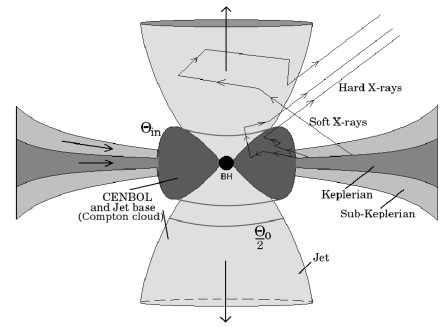
Figure 1: Illustration of the JeTCAF model. The zig-zag arrows show the scattering of photons from the disc and jet. The $\Theta_{o}$ and $\Theta_{\rm in}$ are the solid angle subtended by the outflow and inflow. The figure is adopted from Mondal & Chakrabarti (2021).

4 Results and Discussions

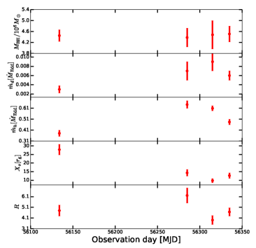
Figure 4: Variation of JeTCAF model fitted parameters with observational epochs.

Figure 2 shows the spectral fitting to the data for four epochs. In all the spectra, we found complex features including absorption lines, skewing of FeK line, soft excess, and some excess at high energies, which can be due to the bulk motion of the outflowing material from the central region or can be due to reflection (as reported by Rivers et al., 2015, and references therein). The model fitted parameters are given in Table 2. The variation of the JeTCAF model fitted parameters are shown in Figure 4. The top panel shows the variation of mass which is constant during the observation period, as expected, however, other parameters changed significantly from second top to bottom panel. The disc or Keplerian accretion rate was $\leq$ 1% of the Eddington rate, however, changed significantly between epochs A to D (second panel). Braito et al. (2014) estimated the mass accretion rate for this source, which is a factor few higher than our estimates. It can be due to either strong dependence of their estimates on the ionized winds and the covering factor they used in their model or due to using higher mass of the BH ($10^{7}M_{\odot}$) and a different accretion efficiency (0.06). The low-angular momentum, hot flow rate was always higher than the Keplerian one. We also noticed that the size of the dynamic corona shrunk from 28 to 10 $r_{g}$. As the size of the corona was changed significantly, and the disc accretion rate was low compared to the halo accretion rate, these are the indication of hard/intermediate spectral state, if the spectra of AGN allow a similar classification as in low mass black hole binaries. Our model fitted shock compression ratio ($R$) varies between 3.9 to 6.2. As the presence of jet was confirmed from [OIII] line that the source has bi-conical outflows (Edmunds et al., 1988), we therefore estimated the mass outflow/inflow rate (dimensionless quantity) using the relation, $R_{\dot{m}}=\frac{\dot{M}_{\rm out}}{\dot{M}_{\rm tot}}=f_{\rm col}f_{0}^{3/2}\frac{R}{4}exp\left[\frac{3}{2}-f_{0}\right]$, where, $f_{\rm 0}=\frac{R^{2}}{R-1}$ (Chakrabarti, 1999), $\dot{M}_{\rm tot}=(\dot{m}_{d}+R\times\dot{m}_{h})$ (Mondal et al., 2014a), and $\dot{M}_{\rm out}$ is the mass outflow rate in $M_{\odot}yr^{-1}$ respectively. The $f_{\rm col}$ value varied between 0.22 to 0.4 (column 7 in Table 2. Our calculated values lie in the range between $0.019\pm 0.006$ to $0.12\pm 0.04$. This gives the mass outflow rate $\sim 0.047$ M_⊙ yr^-1, which is in agreement ($\sim 0.067$ M_⊙ yr^-1) to the independent optical and Chandra imaging studies(Venturi et al., 2018) and the XMM-Newton-RGS data analysis (Braito et al., 2014).

Treating BH mass as a free parameter in JeTCAF we found BH mass is constant (see Figure 4) during the combined XMM and NuSTAR data fitting, that comes out to be $4.38\pm 0.34-4.51\pm 0.29\times 10^{6}M_{\odot}$, closely matches ($4.47\times 10^{6}M_{\odot}$) with the estimation by Onori et al. (2017) and from the molecular gas dynamics ($3.98\times 10^{6}M_{\odot}$) using ALMA data by Combes et al. (2019).

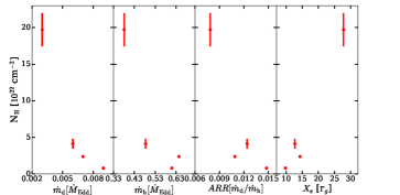
Figure 5: $N_{\rm H}$ decreases with increasing accretion rates, and an opposite profile is observed with the geometry of the corona.

In addition to accretion disc parameters, the ZPCFABS model fitted $N_{\rm H}$ varied (in column 8 of Table 2) by more than an order of magnitude between epochs A to C, and the partial covering fraction ($c_{f}$) was relatively high (see column 9) in all four epochs, however, constant within the error bar. The variation of $N_{\rm H}$ with JeTCAF model parameters are shown in Figure 5. The left panel shows its variation with $\dot{m}_{\rm d}$. A similar variation is observed with the halo rate and accretion rate ration (ARR=disc rate/halo rate). This relative ratio of accretion rates is an indicator of the ratio of disc and corona flux contribution. As the ratio is always $<1$, implies dominant contribution of hot flow rate; thus the radiation coming from the corona is hard. It is quite certain that changing the geometry and accretion flow properties can change the intensity of the radiation emitting from the corona, since it reprocesses photons from the underlying accretion flow. This radiation when falling onto the disc can also influence the disc mass outflow, thus the column density, which can be seen from other panels in Figure 5. The confidence contours of $N_{H}$ with JeTCAF model parameters are shown in Figure 3 in subsection 4.1, which show that the parameters are non-degenerate and robust.

Table 2: Best fitted model parameters are provided in this table. Here, N_H and c_f are hydrogen column density and dimensionless covering fraction. $E_{a}$ and $\sigma_{a}$ are the absorption line energy and width. The superscripts 1 and 2 correspond to the absorption line 1 and 2.

Epoch	$M_{\rm BH}$	$\dot{m}_{\rm d}$	$\dot{m}_{\rm h}$	$X_{\rm s}$	R	$f_{\rm col}$	$N_{H}$	cf	$E_{a}^{1}$	$\sigma_{a}^{1}$	$E_{a}^{2}$	$\sigma_{a}^{2}$	$\chi_{\rm r}^{2}/dof$
	$\times 10^{6}M_{\odot}$	$\dot{M}_{\rm Edd}$	$\dot{M}_{\rm Edd}$	$r_{\rm g}$			$\times 10^{22}$ cm-2		keV	keV	keV	keV
A	$4.45\pm 0.21$	$0.003\pm 0.001$	$0.381\pm 0.028$	$27.8\pm 3.1$	$4.80\pm 0.52$	$0.39\pm 0.08$	$19.72\pm 2.27$	$0.79\pm 0.17$	$2.04\pm 0.12$	$0.91\pm 0.13$	$6.71\pm 0.08$	$0.17\pm 0.06$	641/506
B	$4.38\pm 0.34$	$0.007\pm 0.001$	$0.643\pm 0.034$	$14.3\pm 1.9$	$6.21\pm 0.51$	$0.22\pm 0.03$	$2.38\pm 0.15$	$0.77\pm 0.03$	$2.50\pm 0.02$	$0.11\pm 0.03$	$6.78\pm 0.02$	$0.19\pm 0.02$	1101/704
C	$4.48\pm 0.52$	$0.009\pm 0.002$	$0.609\pm 0.022$	$9.8\pm 1.2$	$3.91\pm 0.42$	$0.38\pm 0.11$	$0.80\pm 0.18$	$0.89\pm 0.08$	$1.87\pm 0.06$	$1.74\pm 0.07$	$6.76\pm 0.02$	$0.21\pm 0.03$	1214/707
D	$4.51\pm 0.29$	$0.006\pm 0.001$	$0.484\pm 0.024$	$12.7\pm 1.6$	$4.67\pm 0.38$	$0.40\pm 0.09$	$4.13\pm 0.67$	$0.87\pm 0.04$	$2.26\pm 0.15$	$0.75\pm 0.10$	$6.62\pm 0.15$	$0.12\pm 0.19$	959/688

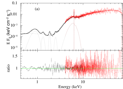
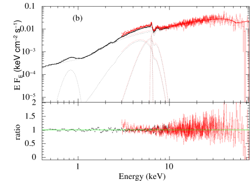
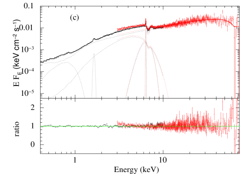
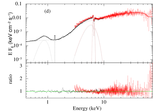
Figure 2: JeTCAF model fitted 0.4$-$75.0 keV spectra for all four epochs of NGC 1365 during XMM-Newton and NuSTAR era. Here, (a-d) corresponds to epochs A to D. The different Gaussian lines are used for emission/excess at different energy range including at $\sim$6.4 keV. The model fits show the absorption line and spectral shape change in each epoch, along with a PCygni profile in the FeK band.

4.1 Robustness of model parameters

Figure 3 shows the confidence contours of $N_{H}$ with other JeTCAF  model parameters. We have used steppar command in XSPEC to generate these plots. Different model parameters are labelled in x-axis. Three different contour colors (red, green, and blue) correspond to one, two, and three sigma confidence level. It is also the same as $\Delta\chi^{2}$ fit statistics of 2.3, 4.61, and 9.21. The correlation of $N_{H}$ with model parameters are clearly visible from the contour plots. The uncertainty of $N_{H}$ fits within 0.6 dex for 2 sigma confidence level. The other parameters assess better precision. The correlations are clear, which show that there is no obvious degeneracy between parameters and the solution is robust.

The top panel shows direct correlation of $N_{H}$, with M_BH, $\dot{m}_{d}$, and $\dot{m}_{h}$, implies that if these parameters value increase, continuum luminosity will also increase, therefore continuum driven wind will also contain more material along the LOS. However, in the case of $X_{s}$ is opposite, as it anti-correlates with the disc accretion rate. In the case of R (up to the strong shock condition value, which is 4; see Chakrabarti, 1999) and $f_{col}$, increase in both the parameters, increase the luminosity contribution from the jet, therefore the wind material launching along the LOS will increase. This gives a positive correlation. We note that in the case of, $f_{col}$ the contour is not closed at its higher value side (the upper limit of the grid value for this parameter is 0.5), this can be an artefact. Our continuum driven wind launching correlation study agrees with the work by Gofford et al. (2015, and references therein), where authors studied (anti)correlation of continuum luminosity with different physical quantities of the wind applicable for a large sample.

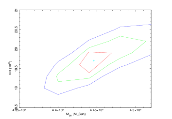
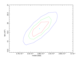
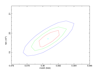
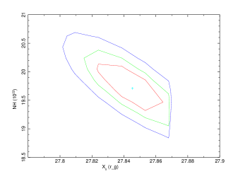
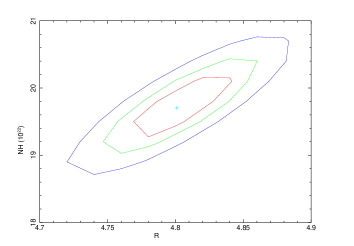
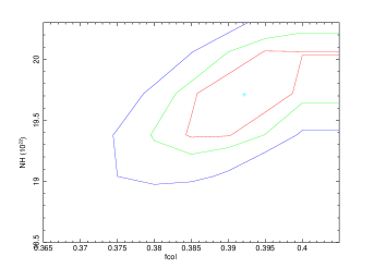
Figure 3: Confidence contour of $N_{H}$ with different continuum model parameters for the epoch A. Three different contour colors show the confidence level of one (red), two (green), and three sigma (blue). Here, x-labels follow the parameter notations used in Table 2, e.g. mdotd, mdoth, and fcol represents $\dot{m}_{d}$, $\dot{m}_{h}$, and $f_{col}$ respectively.

As an additional test, we used photoionization simulation to predict absorption and emission line spectra for the modeled intrinsic spectral energy distributions (SEDs) shown in Figure 6. The SED includes both disc (UV/optical photons), corona, and the jet component (hard X-ray) as discussed in section 3. In JeTCAF model, we compute the EUV photons considering the disc to be multi-temperature at each radius. At the zeroth iteration, the flux emitted from the disc is purely Keplerian (Shakura & Sunyaev, 1973). These seed photons are getting upscattered by the hot corona. As the iterations go on, the interception of corona photons by the disc is taken into consideration, which modifies the original disc temperature. In order to estimate the transmitted spectrum that an observer can measure along the LOS, we performed the numerical simulation of radiation transfer using the photoionization code cloudy17.02 (Ferland et al., 2017). The essential parameters: the spectral energy distribution (SED), gas density $n_{\rm H}$, column density $N_{\rm H}$ are adopted in such a way that satisfies the spectral fitting from Table 2. The illuminating SEDs used in cloudy are the JeTCAF model component from Fig. 2 fitted for each epoch (excluding the other components). The gas density values $n_{\rm H}=2.65\times 10^{10}$, $1.73\times 10^{11}$,$1.47\times 10^{11}$ and $1.01\times 10^{11}$ cm^-3 are taken for the epochs A to D respectively.

Likewise, the column density values, $N_{\rm H}$= $1.97\times 10^{23}$, $2.38\times 10^{22}$, $0.8\times 10^{22}$ and $4.13\times 10^{22}$ cm^-2 are adopted from Column 8 of the Table 2 for the epochs A to D respectively. The models are computed for the two representative cases of ionization parameter $\xi$=$10^{2}$ and $10^{3}$ erg cm s^-1 respectively. The $N_{H}$ and $\xi$ values fall within the range estimated in the literature (Gofford et al., 2013; Walton et al., 2014; Braito et al., 2014, and references therein). The $N_{H}$ values presently obtained are approximated values, as the fit does not consider ionization effects to the continuum. In all of these simulations, we considered the Solar values of the chemical composition, default in cloudy adopted from Grevesse & Sauval (1998). In order to account for the effects of micro-turbulence in absorption-emission lines, typical turbulent velocity $v_{\rm turb}=1000$ kms^-1 is used. Here we are not estimating or quantifying the turbulent velocity rather considering a typical value as a test case to generate the observed lines, however, for a detailed study for this effect we refer the work by Gofford et al. (2013). Note that, only the classical approach of one dimensional radiation transfer with plane-parallel open geometry without the inclusion of relativistic effects are considered. For the details of cloudy applications in various AGN environments and generic definitions of parameters used, we refer the reader to the relevant literature (for e.g. Adhikari et al., 2015, 2019; Adhikari, 2019) and cloudy documentation Hazy files.

The transmitted spectra zoomed in the band $6-9$ keV are presented in the Fig. 7. The results from cloudy simulations show absorption in the region around 6.4 keV, which is similar to that seen in the observed spectra shown in Fig. 2. The change in the spectral shapes, reflected in the illuminating SEDs in cloudy, during the transition from epoch A to epoch D also changes the extent of Fe absorption. For the lowest value of mass accretion rate (0.003 $\dot{M}_{\rm Edd}$) in epoch A, there is a considerable amount of Fe absorption, and it becomes weak as the accretion rate becomes maximum (0.009 $\dot{M}_{\rm Edd}$) in epoch C. This result from basic simulations in cloudy nicely corroborates with the observed features of absorption presented in Fig. 2. However, the emission lines observed are somehow skewed or broadened by the general relativistic (GR) effects of the highly spinning source. These effects are not included in cloudy spectra and thus several components of narrow emission lines are present in Fig. 7. We noticed that the energy at which the absorption is significant depends on the adopted value of the $\xi$ in the photoionization models. The increase in $\xi$ allows for the ionization of the Fe to higher levels and as a result significant absorption towards the higher energy bands are seen. We note that the current CLOUDY modelling is to check whether the model SEDs for a given ionization parameter and turbulent velocity can generate emission and absorption lines similar to what is observed for NGC  1365 or not. However, the current approach does not measure the $\xi$ parameter robustly, it requires a detailed study. We plan to address this issue with grid of photoionization simulations with variations in ionization parameter in the future work.

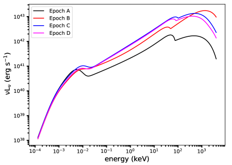
Figure 6: The incident SEDs used in cloudy models for the four epochs considered here. The SEDs are computed using the JeTCAF model which includes relevant physical processes in the accretion disc. The EUV flux is computed assuming the disc is emitting modified multi-color blackbody photons from each radius of the disc.

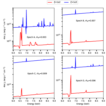
Figure 7: The simulated spectra zoomed between $6$ to $9$ keV for four different epochs using cloudy photoionization code. The evolution of the absorption properties with the change in the disc mass accretion rates (as seen from the fitted data) are plotted in each panel. The red and blue lines correspond to $\xi=$ 100 and 1000 respectively. The micro-turbulence of $v_{\rm turb}=1000$ km s^-1 is used in the simulations for all epochs.

4.2 Failed wind scenario

We consider here the case of the absorber is being associated with the outflowing matter. One of the most prominent outflowing region within AGNs is the broad line region (BLR), it is also one of the candidate to host intervening matter. Studies of warm absorbers (WA) observed at X-rays consider disc outflow or BLR as a source of absorption (Maiolino et al., 2010; Risaliti et al., 2011) or at least one of its component (like NGC 5548 case described by Kaastra et al., 2014). Also, torus can be responsible for part of absorption (Mrk 509 study by Kaastra et al., 2012). The expected ionization parameter value suggested here, ${\rm log}\ \xi\sim 2-3$, agrees with the values expected at the BLR position. Thus, we give here theoretical consideration of the BLR-like outflow. One of the possible outflow scenario is the failed radiatively driven outflow (FRADO) model, which clearly connects the BLR with the underlying accretion disc (Czerny & Hryniewicz, 2011).

We assume that the wind moves away from the disc with constant speed $v_{\rm w}$, in the form of a partial thin spherical shell at a distance $R_{\rm BLR}$ from the central source, the amount of mass per unit time carried out by the wind is:

$$\dot{M}_{\rm w}=\mu m_{p}N_{\rm H}v_{\rm w}R_{\rm BLR}\Omega,$$ (1)

where, $\mu=1.4$, $m_{p}=1.67\times 10^{-24}$ gm, $\Omega=\pi/2$ (Maiolino & Rieke, 1995a), and $R_{\rm BLR}$ are the mean atomic mass per proton, proton mass, typical value of the solid angle subtended by the outflow, and the radius of the BLR respectively. From our spectral fitting, we found that $N_{\rm H}$ decreases with increasing $\dot{m}_{\rm d}$, follows the relation $\mathcal{N}\dot{m}_{\rm d}^{-\beta}$. For NGC 1365, $\mathcal{N}\sim 1.5\times 10^{17}$ cm^-2 and $\beta$, $2.43\pm 0.15$.

To estimate the radial position of the outflowing matter we used an empirical relation based on reverberation mapping results for nearby AGNs (ie. Bentz et al., 2009) which is supported and explained by the FRADO model. The BLR radius can be estimated from Czerny & Hryniewicz (2011),

$$\log R_{\rm BLR}=1.538\pm 0.027+0.5\log L_{44,5100}$$ (2)

where $R_{\rm BLR}$ is in light days and $L_{44,5100}$ is the monochromatic luminosity at 5100 Å ($\lambda L_{\lambda}$) measured in units of $10^{44}$ erg s^-1. We can translate $L_{44,5100}$ to the bolometric luminosity using the relation $L_{\rm bol}=10.33L_{\rm 5100}$ (Richards et al., 2006). The $L_{\rm bol}$ is calculated using the relation $\eta\dot{m}_{d}c^{2}$, where, $\eta=0.1$ is considered. Our estimated values for $R_{\rm BLR}$ (in cm) using Equation 2 are, {$3.61\times 10^{15}$, $5.47\times 10^{15}$, $6.27\times 10^{15}$, and $5.14\times 10^{15}$} for the epochs A to D are consistent with the literature.

As the radiation from the central region falls onto the wind, and considering that on average each emitted photon scatters about once before escaping to infinity, this suggests that the total wind momentum must be of the order of the photon momentum (King, 2010) can be written as

$$\dot{M}_{\rm w}v_{\rm w}\simeq\frac{L_{\rm bol}}{c},$$ (3)

here $c$ is the speed of light.

After solving few steps, we find the equation for the wind velocity as,

$$v_{\rm w}=\frac{L_{\rm bol}^{0.5}\dot{m}_{\rm d}^{\beta/2}}{(\mathcal{N}cm_{p}R_{\rm BLR}\mu\Omega)^{1/2}}=30\left(\frac{L_{\rm bol}\dot{m}_{\rm d}^{\beta}}{\mathcal{N}R_{\rm BLR}}\right)^{1/2}\leavevmode\nobreak\ \leavevmode\nobreak\ \text{km}\leavevmode\nobreak\ \leavevmode\nobreak\ \text{s}^{-1}.$$ (4)

Our estimated wind velocities for all four epochs from A to D are: 1445, 4978, 7235, and 4001 km s^-1 respectively. The estimated wind velocities fall in the range reported in earlier studies on continuum driven wind launching (see Gofford et al., 2013; Braito et al., 2014; Gofford et al., 2015, and references therein). In epochs A and D, the velocity values are less than the wind terminal velocity attained maximum (5748 and 4839 km  s^-1 estimated using $\sqrt{2GM_{\rm BH}/R_{\rm BLR}}$, here, G = Gravitational constant). For the epoch B, wind velocity is comparable with its terminal velocity (4623 km  s^-1) of the wind. This failed wind behaves as a cloud shielding the central emission. However, in epoch C wind velocity higher than the terminal velocity (4365 km  s^-1) can help to drive the material away from the disc, therefore, much less column density was observed. A similar scenario was studied earlier for a low mass black hole binaries (Miller et al., 2020).

From the model fits, the high absorption; variable column density along the LOS, which we argue could be due to the failed wind above the disc surface. The disc accretion rate was low, implies the radiative pressure was also low, therefore the wind launched from the disc could stay in place and the matter was not pushed by the radiation to outer radii. In addition, strong ionizing radiation or outflows (which often is observed in the hard or intermediate spectral states, when accretion rate is low) from the central region of the disc itself can over ionize the wind from the disc, that can prevent the wind being driven away from the disc, therefore its velocity decreases (for an extensive study in Proga & Kallman, 2004). On the other hand, the failed wind BLR model suggests that the outflow velocity scales with the accretion rate. This happens because of its strong connection with the underlying accretion disc. As the dusty matter is pushed away from the disc atmosphere by the radiation from the underlying disc and later is exposed to the central radiation, which breaks its driving force or pushes it away stronger to the outer radii (Naddaf et al., 2021). There are other physical mechanisms that can produce different emission/absorption lines in AGN environment, recently discussed in Laha et al. (2021, for a review).

5 Conclusions

In this paper, we study the changing look active galactic nucleus NGC 1365 using accretion-ejection model including absorption and line emission in order to understand the maximum possible underlying physical processes behind this changing look phenomenon. From our analysis, we conclude that:

• The accretion rates and their ratio, and the size of the dynamic corona varied significantly during the observation period.

• The compression ratio of the shock at the boundary layer of the dynamic corona lies between 3.9 to 6.2, which is used to estimate the mass outflow rate from the dynamic corona. The maximum outflow rate estimated is $\sim 12\%$ of the inflow rate. This confirms the previous findings that the outflows are present in the system.

• The geometry/size of the dynamic corona is also responsible for variable luminosity, that correlates with the hydrogen column density along the line of sight.

• The accretion-ejection model fitted mass is placed within a range between $4.38\pm 0.34-4.51\pm 0.29\times 10^{6}M_{\odot}$, remarkably matches with the estimation by Onori et al. (2017).

• The presence of prominent absorption line and high hydrogen column density is due to low mass accretion rate. The low accretion rate is not able to generate enough pressure to push the matter farther out from the disc (consistent with recent simulation by Naddaf et al., 2021), therefore, it blocks the radiation coming from the inner region. This is also evidenced from the cloudy simulations, where absorption features are stronger (at the highest $N_{\rm H}$) for the low mass accretion state. This explains the “failed wind” scenario due to low wind velocity.

• We studied the correlation between $N_{H}$ with other model fitted continuum parameters (see subsection 4.1) and found that they are consistent with the physical picture of the model and agree with the earlier works on continuum driven wind launching (Gofford et al., 2015, and references therein).

• Therefore, CLAGNs can show significant variability if the accretion rate and the corona geometry change substantially.