Flux and spectral variability of Mrk 421 during its moderate activity state using NuSTAR: Possible accretion disc contribution?

Abstract

Context. The X-ray emission in BL Lac objects is believed to be dominated by synchrotron emission from their relativistic jets. However, when the jet emission is not strong, one could expect signatures of X-ray emission from inverse Compton scattering of accretion disc photons by hot and energetic electrons in the corona. Moreover, the observed X-ray variability can also originate in the disc, and gets propagated and amplified by the jet.

Aims. Here, we present results on the BL Lac object Mrk 421 using the Nuclear Spectroscopic Telescope Array data acquired during 2017 when the source was in a moderate X-ray brightness state. For comparison with high jet activity state, we also considered one epoch data in April 2013 when the source was in a very high X-ray brightness state. Our aim is to explore the possibility of the signature of accretion disc emission in the overall X-ray emission from Mrk 421 and also examine changes in accretion parameters considering their contribution to spectral variations.

Methods. We divided each epoch of data into different segments in order to find small scale variability. Data for all segments were fitted using simple powerlaw model. We also fitted the full epoch data using the two component advective flow model to extract the accretion flow parameters. Furthermore, we estimated the X-ray flux coming from the different components of the flow using the lowest normalization method and analysed the relations between them. For consistency, we performed the spectral analysis using available models in the literature.

Results. The simple powerlaw function does not fit the spectra well, and a cutoff needs to be added. The spectral fitting of the data using the two component advective flow model shows that the data can be explained with a model where (a) the size of the dynamic corona at the base of the jet from $\sim 28$ to $10\leavevmode\nobreak\ r_{s}$, (b) the disc mass accretion rate from 0.021 to 0.051 $\dot{M}_{\rm Edd}$, (c) the halo mass accretion rate from 0.22 to 0.35 $\dot{M}_{\rm Edd}$, and (d) the viscosity parameter of the Keplerian accretion disc from 0.18 $-$ 0.25. In the assumed model, the total flux, disc and jet flux correlate with the radio flux observed during these epochs.

Conclusions. From the spectral analysis, we conclude that the spectra of all the epochs of Mrk 421 in 2017 are well described by the accretion disc based two component accretion flow model. The estimated disc and jet flux relations with radio flux show that accretion disc can contribute to the observed X-ray emission, when X-ray data (that covers a small portion of the broad band spectral energy distribution of Mrk 421) is considered in isolation. However, the present disc based models are disfavoured with respect to the relativistic jet models when considering the X-ray data in conjunction with data at other wavelengths.

1 Introduction

Active galactic nuclei (AGN) harbour a supermassive black hole at their center. They emit X-rays from their very central region and are believed to be powered by accretion of matter onto supermassive black holes ($\sim 10^{6}-10^{10}M_{\odot}$) located at the centre. The process of accretion leads to AGN emitting copious amount of radiation (luminosity $\sim 10^{42}-10^{48}$ erg s^-1) as well as producing a variety of highly energetic phenomena (Lynden-Bell, 1969; Shakura & Sunyaev, 1973; Rees, 1984). A majority of AGN emit little to very low radio-emission and are called radio-quiet AGN, while a minority emit ample radiation in the radio band and are called radio-loud AGN (Kellermann et al., 1989). However, recently, it has been proposed that AGN can be better divided based on their physical differences (Padovani, 2017) into non-jetted AGN (ones that lack strong relativistic jets) and jetted AGN (ones with strong relativistic jets). Among the jetted AGN are blazars, a peculiar category characterised by an extreme flux variations across the entire electromagnetic spectrum over a range of timescales from minutes to days (Wagner & Witzel, 1995; Ulrich et al., 1997), flat spectra in the radio band, and high optical polarization and polarization variability (Angel & Stockman, 1980; Andruchow et al., 2005; Rakshit et al., 2017). Such characteristics are now attributed to their relativistic jets oriented close to the line of sight to the observer and are subjected to Doppler boosting.

Blazars are divided into two categories, namely, flat spectrum radio quasars (FSRQs) and BL Lac objects (BL Lacs). This division is historically based on the presence or absence of emission lines in the spectra of those objects. FSRQs have emission lines in their optical/infrared spectra, while BL Lacs have either weak emission lines (equivalent width $<$ 5 Å) or featureless spectra (Urry & Padovani, 1995). It is now believed that FSRQs are powerful sources with strong relativistic jets and powered by the standard optically thick and geometrically thin accretion disc. On the other hand, BL Lacs are weak sources with radiatively inefficient and geometrically thin accretion disc. In such discs, the reduced ultra-violet (UV) emission might not be able to photo-ionise the broad line region (BLR) leading to weak or absent broad emission lines in BL Lacs (Ghisellini, 2019).

Alternatively, the weakness or absence of emission lines in the spectra of BL Lacs could be understood in the context of the continuum getting enhanced due to Doppler boosting, and becoming dominant during the increased jet activity of BL Lacs. It has been shown by Foschini (2012) that the faint lines detected in BL Lacs could be due to the combined effect of the boosted jet emission and a weak accretion disc. Removal of the contribution of the boosted jet emission to the continuum leads to emission lines in BL Lacs having FWHM similar to that of other AGN. This finding leads to hypothesize that during the low jet activity or faint state of BL Lacs, the observed X-ray emission could have significant contribution from the inverse Compton (IC) scattering of soft photons from the accretion disc off the “hot corona”, in addition to the synchrotron emission from the relativistic jet. According to Ghisellini et al. (2011) a physical distinction between FSRQs and BL Lacs can be made based on the ratio of the luminosity of the BLR to the Eddington luminosity ($L_{\rm BLR}/L_{\rm Edd}$) with FSRQs having $L_{\rm BLR}/L_{\rm Edd}$ greater than 5 $\times$ $10^{-5}$ compared to BL Lacs.

The broad band spectral energy distribution (SED) of blazars, shows two prominent peaks, one peaking around radio-optical-X-ray frequencies and the other one peaking at X-ray to GeV $\gamma$-ray energies. In the leptonic scenario of emission from blazar jets, the low energy peak is attributed to synchrotron emission process, while the high energy peak is attributed to IC process. Also, based on the location of the synchrotron peak in the SED, blazars are further divided in low synchrotron peaked (LSP; $\nu_{\rm peak}<10^{14}$ Hz), intermediate synchroton peaked (ISP; $\nu_{\rm peak}=10^{14-15}$ Hz) and high synchrotorn peaked (HSP; $\nu_{\rm peak}>10^{15}$ Hz) blazars. The observed X-ray emission in blazars is mostly by synchrotron or synchrotron self Compton (SSC) processes, and thus jet dominated. Therefore, the X-ray flux variations in them are believed to be due to their relativistic jets. However, in the non-jetted category of AGN such as Seyfert galaxies the observed X-ray emission is predominantly due to inverse Compton scattering of optical/UV photons from the accretion disc by energetic electrons in the corona and thus the X-ray flux variations in them is attributed to the accretion disc (Haardt & Maraschi, 1993).

In the faint or low jet activity state of FSRQs, prominent accretion disc emission is seen in the broad band SED (Raiteri et al., 2009) in many sources and therefore in their faint state, their observed X-ray emission could also have a contribution from the accretion disc/corona. Similarly, in the case of BL Lacs too, continuum emission is dominated by non-thermal emission from their relativistic jets. However, occasionally broad emission lines are seen in their optical spectra which suggests that the BLR is photoionised by the accretion disc emission. Emission lines (though weak) are seen in many BL Lac objects (Raiteri et al., 2009; Vermeulen et al., 1995; Corbett et al., 2000; Stocke et al., 2011). Also, broad emission lines are seen in many $\gamma$-ray detected BL Lacs (Shaw et al., 2013), a large fraction of them belonging to the LSP and ISP category. Recently, from X-ray observations carried out on the BL Lac object Mrk 421 Chatterjee et al. (2018) found a break in the power spectral density, which the authors attributed to the influence of the disc onto the jet emission from Mrk 421. In the X-ray light curves of many blazars, log normal (LN) flux distribution is observed similar to that seen in Seyfert galaxies (Ackermann et al., 2015; Sinha et al., 2016) which again argues for the contribution from the accretion disc to the observed X-ray emission of blazars. According to Wandel & Urry (1991), the observed UV and X-ray emission from BL Lacs can come from accretion disc. They were able to fit the observed UV and soft X-ray spectrum of the BL Lac object PKS 2155$-$304 using accretion disc spectra. Also Grandi & Palumbo (2004); Zdziarski & Grandi (2001) found the signature of accretion disc emission in the X-ray spectra of the blazar 3C 273 and rthe adio galaxy 3C 120. However, this model of Wandel & Urry (1991) was not supported by Smith & Sitko (1991), who from optical polarimetric observations on the BL Lac PKS 2155$-$304, claimed to have found no observational evidence for the contribution of the accretion disc to the observed UV and optical continuum. A long term multi-wavelength lightcurve and SEDs study showed that the data fits well with the LN model, inferred the lognormality character might have originated from the disc and amplified by the jet (Kapanadze et al., 2020; Acciari et al., 2021).

Mrk 421 (z = 0.03 de Vaucouleurs et al. 1991) is one of the closest BL Lac objects hosted in an elliptical galaxy at a distance of 140 Mpc ($H_{0}$= 71 km $s^{-1}$ $Mpc^{-1}$, $\Omega_{m}$ =0.27, $\Omega_{\Lambda}$ = 0.73) and hosting a 4$\times$ $10^{8}$ $M_{\odot}$ black hole (BH) at the center (Wagner, 2008). The SED of Mrk 421 has the classical two-peak shape (Urry & Padovani, 1995; Ulrich et al., 1997) and it has been studied extensively in a broad energy band ranging from radio to very high energy $\gamma$-rays (Fossati et al., 2008; Abdo et al., 2011; Shukla et al., 2012; Aleksić et al., 2015). Most of the observed properties of Mrk 421 are understood to arise from a relativistic jet at a small angle along our line of sight (Urry & Padovani, 1995). There are frequent multiwavelength (MWL) campaigns on this object to understand its multiscale variability (Macomb et al., 1995; Gupta et al., 2004; Acciari et al., 2009; Paliya et al., 2015; Pandey et al., 2017, and references therein). It is an HSP BL Lac and is also the first extra-galactic source detected in TeV $\gamma$-rays (Punch et al., 1992). As suggested by several studies, the X-ray spectra of HBLs are curved and described well with the log-parabola model (Massaro et al., 2004; Tramacere et al., 2007), where the photon index is not a constant, rather varies with logarithmic energy. In 2006, the source was observed with a peak flux of $\sim 85$ mCrab in the 2$-$10 keV band, indicating that the first peak of SED occurred at an energy beyond 10 keV (Tramacere et al., 2009; Ushio et al., 2009). Again, in 2013 April, Mrk 421 was observed to undergo a major X-ray outburst and was extensively studied by multiple observational facilities, including the Nuclear Spectroscopic Telescope Array (NuSTAR) and Swift satellites. Mrk421 showed very high optical emission during its historically low X-ray emission during January-February 2013 and the presence of multiple compact regions contributing to the broadband emission during low-activity states was suggested by Baloković et al. (2016). On the contrary, low optical emission during high X-ray emission was also reported during in February 2010 by (Abeysekara et al., 2020). Therefore, the optical and X-ray emission are found to show different behaviour (Carnerero et al., 2017). A MWL study has been performed using the radio to TeV energy band data, very recently, where the authors studied (anti)correlation between optical and hard X-ray energy bands (MAGIC Collaboration et al., 2021). Also, it has been studied for its X-ray and $\gamma$-ray flux variability characteristics (Kapanadze et al., 2016; Rani et al., 2017, 2019; Rajput et al., 2020).

A huge amount of MWL data available on BL Lacs are well explained assuming the centre is viewed along the jet. In such a view, though the jet emission significantly gets Doppler boosted, one can also see the central region of BL Lacs. Therefore, it is quite natural to expect contributions of both the accretion disc in the UV/optical emission and corona in the observed X-rays. When the jet emission dominates, it might not be possible to find the signature of the accretion disc/corona in the continuum emission from BL Lacs. However, when the jet is less active, emission from accretion disc/corona could form a significant component of the observed continuum emission. Weak (equivalent width $<$ 1 Å) and narrow FWHM = $300\pm 30$ km/sec) Ly$\alpha$ emission line has been seen in Mrk 421 by Stocke et al. (2011). The weakness of the Ly$\alpha$ line in Mrk 421 could be due to the combined effects of (a) the Doppler boosting of the continuum emission by the relativistic jet that is closely aligned with the observer and (b) weak accretion disc. Taking Doppler boosting into account, the intrinsic FWHM of Ly$\alpha$ line in Mrk 421 was found to be similar to other AGN (Foschini, 2012). These observations clearly demonstrate that during the faint state of BL Lacs, the accretion disc/corona emission too can be an important contributor to the observed X-ray emission, however, might not dominate the non-thermal emission from the jet. In a detailed multiwavelength study by Acciari et al. (2021) showed that the flux distributions of Mrk 421 in radio and soft X-rays are better described with a Gaussian function, while in the optical, hard X-rays, high energy and VHE $\gamma$-rays are preferably described with a LN distribution. Such distribution of flux implies that the emission is being powered by a multiplicative process rather than an additive one. In addition, Chakrabarti & D’Silva (1994) mentioned that very high energy $\gamma$-rays from blazars could be due to Fermi acceleration taking place at the surface of the CENtrifugal pressure supported BOundary Layer (CENBOL) of a thick disc. Here, CENBOL behaves like a dynamical corona also a base of the jet (see Mondal & Chakrabarti, 2021). At this point, it is worth questing whether a static corona or normal corona can explain the same behaviour? The answer is no, as the normal corona cannot remain hot for ages unless heated by some underlying heating mechanism. It has been observed that spectral index steepens with age (Saikia et al., 2016, and references therein), because jets are not reheated and only cools down with age. Therefore, it is essential to consider a dynamical advective halo or dynamic corona to replenish the electrons. Considering the above observed and theoretical constraints, in this work, we aimed to fit the observed X-ray spectra of Mrk 421 during its moderately X-ray brightness state with disc based models to derive various disc parameters which could provide useful inputs into the accretion characteristics of Mrk 421. However, we note that in the literature, X-ray emission from Mrk 421 is explained by processes that do not arise from the disc (MAGIC Collaboration et al., 2021, and references therein). This paper is organized as follows: in Section 2 we explain the observations and data reduction procedures, in Section 3, we discuss the various analysis carried out on the data sets. The conclusions are given in the final Section.

2 Observation and data reduction

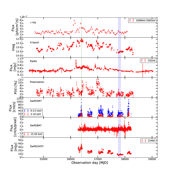
Figure 1: Long term flux and polarization variation of the source. From top, we show the flux variation in the $\gamma$-ray, optical and radio bands. The bottom panel shows the variation in the degree of polarization (%) in the optical V-band.The blue dashed lines show the epochs of NuSTAR observations studied here. The green dotted line correspond to data taken during April 2013. The bottom three panels show the fluxes from the Swift observation. The X-ray and UV light curves are taken from Arbet-Engels et al. (2021).

Mrk 421 was in its moderate brightness state in the radio (a proxy for jet emission) during 2017 and high brightness state during 2013. We show in Figure 1, its MWL light curves, that include the one month binned $\gamma$-ray light curve for the energy range 100 MeV to 200 GeV from the Fermi Gamma-ray Space Telescope, the optical V-band light curve from Steward Observatory (Smith et al., 2009) and the 15 GHz radio light curve from the Owens Valley Radio Observatory (OVRO; Richards et al. 2011). The V-band light curve was directly taken from Steward archives and we have not done host galaxy correction to the photometric points. Also shown in the same figure is the degree of polarization in the optical V-band. From the soft X-ray light curve from the Swift/XRT and the hard X-ray light curve from the Swift/BAT (Arbet-Engels et al., 2021) it is evident that Mrk 421 was in a moderate X-ray brightness state during the year 2017 compared to previous years. The vertical dotted lines in Figure 1 show the epochs considered in the present paper. Analysis of the X-ray data available during the low jet activity state of the source through accretion disc based models fits to the observed X-rays could be a way to derive various accretion disc parameters of the source. We therefore searched the archives of the NuSTAR (Harrison et al. 2013) for the availability of X-ray data and could find four epochs of both data available during the same period. For comparison, we also selected one epoch during 2013, when the source was in a bright jet activity state that yielded high and variable X-ray and $\gamma$-ray emission (Paliya et al., 2015; Acciari et al., 2020). The details of the observations are given in Table 1. The flux of the source in the optical, X-ray, and $\gamma$-ray bands and the optical polarization during those four epochs are given in Table 2. From Table 2, it is to be noted that though the source is detected in the $\gamma$-ray band with good test statistics (TS) values, it is in a relatively quiescent state (see Figure 1).

Considering the historic brightness state of the source, it is likely that the source is in a relatively faint state in the optical in 2017. Carnerero et al. (2017) presented the optical light curves during 2008 - 2015 in R-band. The lowest brightness state was in 2008, when the R-band brightness was  13.5 mag. The R-band brightness during the four epochs range between 13.09 and 13.32 mag, which suggest that during the four epochs considered in this work, the R-band brightness is close to the historic faint state of Mrk 421. Low optical emission can always be not a proxy for low X-ray emission as a flare in X-ray can have no corresponding flare in the optical. In such cases, the optical and X-ray emission may not be co-spatial (Carnerero et al., 2017). On the contrary, there can be instances of an optical flare with no counterpart in the X-ray band. Also, the multi-band flux variability characteristics of blazars are highly complex, as revealed from recent observations Rajput et al. (2019, 2020, 2021). However, inspection of Figure 1 indicate that the source is in a relatively faint state across different bands of the electromagnetic spectrum during 2017. Thus, during 2017, the contribution of relativistic jet to the total emission in the optical/UV/X-ray may be relatively lower compared to the high jet activity state in 2013.

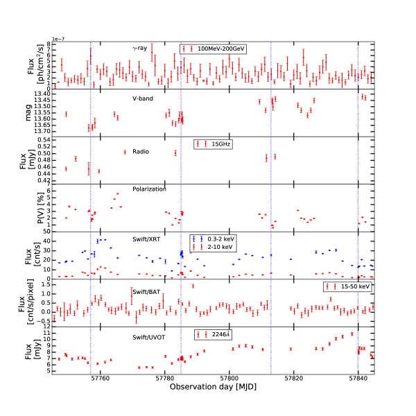
Figure 2: Zoomed version of Figure 1, depicting clearly the brightness states of the four epochs analysed in this work.

The baseline gamma-ray flux (Figure 1) is $\sim 2\times 10^{-7}$ ph cm^-2 s^-1. During epochs C and D, the gamma-ray activity state is also close to this value. Considering the X-ray light curves from December 2012 - April 2018, the minimum 0.3-2 keV X-ray flux was 5.71 ph s^-1 and the maximum 0.3-2 keV X-ray flux was 117.44 ph s^-1. During January - December 2017, the minimum and maximum flux values were 8.84 and 41.64 ph s^-1 respectively. During the epochs analysed in this work, the flux values ranged between 13.27 and 26.73 ph s^-1 (Table 2). The source is thus not in the faintest X-ray state; however, the X-ray flux values are much weaker than other times and hence the contribution of jet emission during these four epochs is relatively lower compared to other epochs. Also, during the period the $\gamma$-ray, optical and X-ray variations are correlated, and they are also at the moderate brightness states. Between epoch E (historic bright state; fluxes are given in subsection 3.4) and D, the soft flux has decreased by 5.8 times, and the hard (2-10 keV) flux has decreased by 22.6 times. The reduction of hard flux between E and D is much larger, followed by soft X-ray. This points to relatively lower dominance of jet emission in epoch D compared to E and emerging contribution of UV emission from the accretion disc. Between epochs B and D, the hard X-ray flux has decreased by a factor of $\sim 3.5$, while the UV flux has increased by a factor of 1.2. The moderate brightness state in the optical, $\gamma$-ray and radio bands along with low optical polarization in comparison to the polarization at the high X-ray brightness state in 2013 (see Figure 1 and Figure 2) indicates that the jet activity in Mrk 421 during 2017 is likely to be lower. The $\gamma$-ray lightcurve in Figure 2 is one day binned. There are also reports in the literature that point to varied correlation between optical flux and degree of optical polarization (Gaur et al., 2012; Pandey et al., 2021).

Models available in the literature on polarization in blazars point to shock propagation through twisted fields inside the jet being the cause of the changes in polarization (Blandford & Königl, 1979; Lyutikov et al., 2005; Marscher et al., 2008; Itoh et al., 2016, and references therein). In the present study, of the four epochs considered, in three epochs namely A to C, the source was at a moderate X-ray brightness state, and larger than the typical average X-ray brightness over a quiescent 4-5 months period (Abdo et al., 2011). But during epoch D, the X-ray brightness of the source was lower than the typical average quiescent brightness. Also, multi-band SED modelling coupled with other analysis point to the presence of multiple emission zones that give rise to the observed emission even during the quiescent state (Baloković et al., 2016). Such multiple emission regions contributing to the overall observed emission too will give rise to the low level of optical polarisation typically observed in this source, except during instances that are close to flaring episodes. Given the presence of multiple emission regions contributing to the observed broad band emission during the quiescent state of Mrk 421, we aim to explore the possibility that there is disc emission in the observed X-ray spectrum and under this hypothesis deduce various accretion parameters of the source. We therefore aim to use the Two Component Advective Flow Two Component Advective Flow (tcaf; Chakrabarti & Titarchuk, 1995) model on the four sets of data analysed in this work. However, we note that multi-band SED fitting of the observations both in quiescent and flaring states invoke SSC processes for the observed X-rays. Recently Jana et al. (2017) estimated jet flux from tcaf model for systems where the lowest contribution can be treated from the disc only (and that too not boosted by Doppler effect) while the brightest part will have both the disc and the jet. Figure 3 shows the optical spectra of the source taken from the Steward Observatory (Smith et al., 2009) archives for the epochs considered in this present study. The combined spectrum of the four epochs is shown in black. The positions of the H$\alpha$ and H$\beta$ lines are marked with vertical dashed lines and zoomed at the upper and lower corners. The emission lines are not visible in the optical spectra taken during those four epochs using a moderate size optical telescope. This indicates that even in the moderate X-ray brightness state, the Doppler boosted jet emission dominates to swamp the emission lines. Alternatively, high S/N observations with larger aperture telescopes, might have detected faint emission lines. The NuSTAR data were extracted using the standard NUSTARDAS v1.3.1 software. We ran nupipeline task to produce cleaned event lists and nuproducts to generate the spectra. We used a region of $30^{\prime\prime}$ for the source and $50^{\prime\prime}$ for the background using ds9. The data were grouped by grppha command, with a minimum of 30 counts rate per energy bin. The same binning was used for all the observations.

As blazar variability timescales can range from hours to minutes depending on the underlying physical processes (Aharonian et al., 2007; Paliya et al., 2015), we split each epoch of observation into different segments, with each segment containing $\sim 1.8$ ksec of data. This division of the data into segments is to investigate spectral variations in hourly time scale. For that purpose, first we made our own GTI files for each time range using the gtibuild task in SAS environment and used those GTI files during the pipeline extraction (same as in Mondal & Chakrabarti, 2019). As the data quality in each segment is highly noisy above 20 keV, for the analysis of the data pertaining to each segment we used the data in the energy range of 3$-$20 keV. However, considering each epoch of observation as unique, the data is of good S/N up to 60 keV, and therefore, for analysis of each epoch of observation we used the data in the energy range of 3$-$60 keV. For spectral analysis of the data, we used XSPEC (Arnaud, 1996) version 12.11.0. Each segment of the data was fitted using the simple power-law (pl) model, while each epoch of observation was fitted using an accretion disc based tcaf model and the thermal Comptonization model thcomp and the pl model. We used the absorption model ${\it tbabs}$ (Wilms et al., 2000) with the Galactic hydrogen column density fixed at 1.5$\times$ 10²⁰ atoms cm^-2 (Elvis et al., 1989; Kalberla et al., 2005) throughout the analysis.

Table 1: Log of observations.

OBSID	Epoch	Date	MJDstart	MJDend	Exposure (s)
60202048002	A	03-01-2017	57756.99385	57757.52163	23691
60202048004	B	31-01-2017	57784.99038	57785.55288	21564
60202048006	C	28-02-2017	57812.92441	57813.49733	23906
60202048008	D	27-03-2017	57839.91052	57840.63969	31228
60002023031	E	14-04-2013	56396.90355	56397,29939	15605

Table 2: Flux and polarization values of Mrk 421 during the epochs studied in this work. The $\gamma$-ray fluxes are in units of 10^-7 ph cm^-2 sec^-1. The optical flux and polarization measurements during ^a and ^b belong to 27 February 2017 and 28 March 2017. The Soft and Hard represent the Swift/XRT 0.3-2 keV and 2-10 keV band fluxes.

Epoch	Date	$\gamma$-ray	TS	Radio	V-band		R-band	Soft	Hard	UV	Hard/Soft
		flux		mJy	(mag)	pol. (%)	(mag)	ph$s^{-1}$	ph$s^{-1}$	ph$s^{-1}$
A	03 Jan. 2017	3.4	97	$0.46\pm 0.02$	$13.67\pm 0.03$	$2.98\pm 0.06$	$13.32\pm 0.03$	$26.68\pm 0.26$	$6.42\pm 0.07$	$--$	0.24
B	31 Jan. 2017	2.1	29	$0.50\pm 0.01$	$13.61\pm 0.02$	$1.31\pm 0.06$	$13.26\pm 0.02$	$26.73\pm 1.78$	$6.46\pm 0.77$	$7.05\pm 0.11$	0.24
C	28 Feb. 2017	6.9	19	$0.49\pm 0.01$	$13.55\pm 0.02^{a}$	$2.52\pm 0.06^{a}$	$13.19\pm 0.03$	$25.48\pm 0.85$	$6.46\pm 0.42$	$--$	0.25
D	27 Mar. 2017	2.7	11	$0.48\pm 0.01$	$13.42\pm 0.02^{b}$	$1.43\pm 0.05^{b}$	$13.09\pm 0.02$	$13.27\pm 0.44$	$1.88\pm 0.26$	$8.71\pm 0.21$	0.14

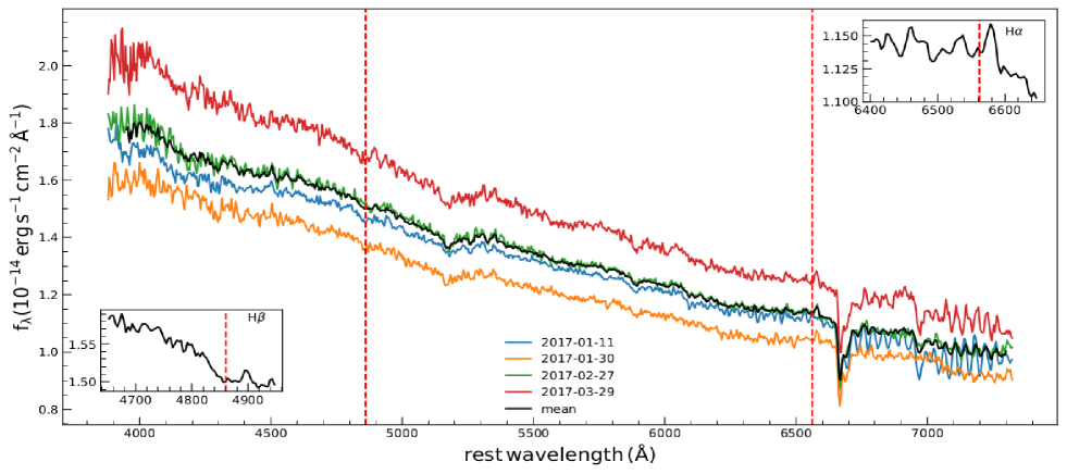
Figure 3: Optical spectra taken from Steward Observatory during the same observation period as considered in NuSTAR analysis. Four different colors correspond to four epochs considered for X-ray analysis and the black curve shows the combined spectrum. Zoomed regions around H$\alpha$ and H$\beta$ lines are also shown at the top right and bottom left.

3 Spectral analysis

3.1 Model fits to the spectra

First, we carried out simple pl model fits to each segment of the data in all the epochs. The tbabs*pl model fits the data satisfactorily, with reduced $\chi_{r}^{2}$ between 0.5$-$1.5. The model parameters and the reduced $\chi_{r}^{2}$ for all the segments are given in Table 3. Secondly, for all the data in each epoch of observations, we extracted the spectra in the 3$-$60 keV band and fitted them with both accretion disc and thermal Comptonization models.

For the data belonging to each epoch of NuSTAR, fitting the spectra with the phenomenological pl model (tbabs*pl), was found not to be satisfactory with $\chi_{r}^{2}>1.2$ (see Table 4), except for epoch D, where it was unity. We further fit the NuSTAR data using cutoffpl model, which returns a good fit with $\chi_{r}^{2}\sim 1$. We hypothesize this as a signature of a multiprocess system where disc and jet both can contribute. It is worth mentioning that considering the MWL observation up to TeV band requires synchrotron process based models to fit and infer the data and variability, which are believed to be originated from the jet (see MAGIC Collaboration et al., 2021, for a very recent study). Also, in the literature, the X-ray spectrum in blazars are known to derive from the conventional power law form with a tendency of show curvature, which is generally attributed to synchrotron cooling break (see Gaur, 2020, and references therein).

In the literature about blazars, curved X-ray spectra are common and normally used whenever the X-ray instrumental resolution allows to detect such curvature(see e.g., Massaro et al., 2004). Here we provide a different view based on the discussions in the literature (see earlier sections) that variability originated in the disc can be amplified by the jet. Hence, following our hypothesis, where the accretion disc-based model can be applied to Mrk 421 data during its low or moderate jet activity state. We therefore used the thermal Comptonization model thcomp (Zdziarski et al., 2020) along with partial ionization zxipcf (Reeves et al., 2008) and diskbb as tbabs*zxipcf*thcomp*diskbb to fit the NuSTAR data, which returned good fits. For proper representation and estimation of parameters of the thcomp model, we used “energies” command to extend the energy range from 0.01 to 1000 keV. During the fitting we kept the ionization rate (log $\xi$) to 0.0 for the zxipcf model and the scattering fraction ($f_{\rm sc}$) was kept fixed at 1 for all epochs for the thcomp model. Addition of diskbb provided the temperature of the disc ($T_{\rm in}$) which was found to be reasonable (see Table 5). For epoch D, the partial covering factor ($C_{f}$) was the lowest $0.07$ and the temperature of the corona was the lowest among the four epochs. This implies increased generation of disc photons, which on getting inverse Compton scattered by the hot electrons in the corona cooled the corona down. This is also consistent with the lowest-flux state of the source at epoch D. We found temperature of the corona with values of 144$\pm$46, 55$\pm$8, 51$\pm$9, and 27$\pm$5 keV for epochs A, B, C, and D respectively, thus decreasing. We thus found the temperature of the corona to decrease from epoch A to D. The results of the best fitted model parameters are given in Table 5. From the diskbb model fitted norm we estimated $R_{\rm in}$/$r_{\rm s}$, which comes out to be 57, 25, 17, and 2 for epochs A to D. The estimated values are significant and as per our hypothesis, this could be a signature of the presence of possibly a truncated disc component.

Further, to study the accretion flow parameters and geometrical variation of the flow and its contribution to the spectrum, we fitted the four observations in the 3$-$60 keV band using the physical tcaf model. For spectral fitting, we ran the source code directly in XSPEC as a local model. The tcaf model (Chakrabarti & Titarchuk, 1995) can successfully fit the X-ray data on low mass X-ray binaries (Debnath et al. 2014, and references therein; Mondal et al. 2014, and references therein; Iyer et al. 2015, and references therein; Debnath et al. 2015, and references therein) and AGN (Mandal & Chakrabarti, 2008; Nandi et al., 2019; Mondal & Stalin, 2021), and has been used to infer the outburst behaviour as well as the variability properties of compact objects. This model requires five parameters, namely, (i) mass of the black hole ($M_{\rm BH}$), (ii) disc accretion rate ($\dot{m}_{d}$), (iii) halo accretion rate ($\dot{m}_{h}$), (iv) shock location, which is the boundary of the CENBOL (Chakrabarti (1989), $X_{s}$ in unit of $r_{s}$, where $r_{s}$ is the Schwarzschild radius, $2GM_{\rm BH}/c^{2}$), and (v) shock compression ratio ($R$). For tcaf model fits, we froze the mass of the BH at $4\times 10^{8}$ M_⊙ (Wagner, 2008), which gives $r_{s}=1.2\times 10^{14}\text{cm}$. The quality of fits for all epochs appear to be good with the reduced $\chi_{r}^{2}$ ranging from 0.9 to 1.1. It can be seen that the accretion rate of the disc component varies in the range from 0.02$-$0.05$\dot{M}_{\rm Edd}$ and the halo accretion rate varies from 0.22$-$0.35$\dot{M}_{\rm Edd}$. Increase of the disc accretion rate leads to increase in the number of soft photons. This cools the corona by inverse Compton scattering, thus causing the inner edge of the disc to move inward from $\sim 20$ to $10r_{s}$. The results of the tbabs*zxipcf*tcaf model fits are given in Figure 4. From the parameters obtained from tbabs*zxipcf*tcaf fits to the data we derived post-facto values of $kT_{e}$ of 189, 55, 38, and 20 keV for epochs A, B, C, and D respectively. We are not using any simple equation to calculate $kT_{e}$ in the source code, which depends on all input parameters. Therefore, estimating error is beyond the scope of this paper.

Thus, from the fitting of four epochs of data with both thcomp and tcaf models we infer the following (i) tcaf model alone is a good representation of the observations in the full energy band, proving different accretion flow parameters, (ii) the thermal Comptonization thcomp model along with diskbb well fits the data providing values of the temperature the corona, photon index, and the temperature of the disc, (iii) the nature of variation of $kT_{e}$ is in agreement with the variation in mass accretion rate, (iv) the highest accretion rate obtained for the epoch D from tcaf is in agreement with the lowest flux, and shock compression ratio observed, (v) the adequacy of non-magnetic disc models to fit the data, can be the signature of low magnetic field.

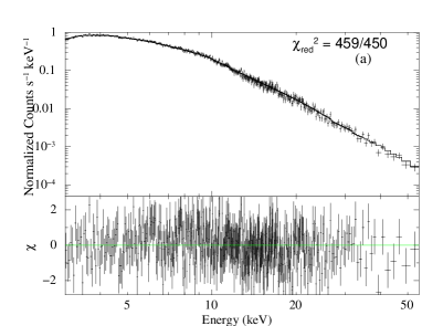
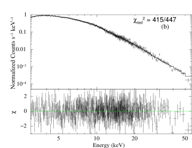
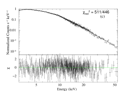
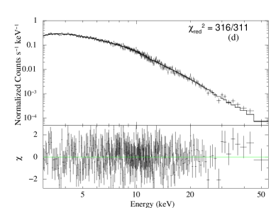
Figure 4: The 3$-$60 keV spectra fitted with tbabs*zxipcf*tcaf model along with the residuals. The panels (a)-(d) correspond to the data acquired at epochs A, B, C and D respectively.

3.2 Photon index and spectral flux

On hourly time scales, the photon index ($\Gamma_{\rm PL}$) is found to vary between $2.2$ and $3.0$ ($\Delta\Gamma=0.8$) within a span of 83 days from epoch A to D. We note that $\Gamma_{\rm PL}$ was always high, which implies that the source was in a high/soft spectral state. The very low flux spectrum with high $\Gamma_{\rm PL}$ belongs to epoch D. Figure 5, left panel shows the variation of $\Gamma_{\rm PL}$ with segments of every epoch of observation. Significant change in $\Gamma_{\rm PL}$ was observed during epoch D. On each epoch of observation, the source exhibited small scale fluctuations in $\Gamma_{\rm PL}$. The green shaded band shows the error bar and black vertical lines show transition in each epoch. To check the behaviour of $\Gamma_{\rm PL}$ of all the segments with the total flux in the 3$-$20 keV band, we plotted the variation of $\Gamma_{\rm PL}$ with the total flux $F_{3-20\leavevmode\nobreak\ keV}$ in Figure 5. We fitted the observed data points in the $\Gamma$ vs. flux diagram using a linear function of the form $\Gamma=a\times F_{3-20keV}+b$, taking into account the errors in both $\Gamma$ and flux following Press et al. (1992). This fitting gave a significant negative correlation between $\Gamma$ and flux with a correlation co-efficient of $-$0.860, i.e. the value of photon index decreases with increasing flux indicating a ‘harder when brighter’ trend in the 3$-$20 keV band. The same behaviour has also been observed using the same data by MAGIC Collaboration et al. (2021). Such behaviour is more often seen in the HSP category of blazars (Giommi et al., 1990; Pian et al., 1998). Mrk 421 is an HSP blazar and the harder when brighter trend could be most likely due to change in the power-law component of the relativistic jet (Rani et al., 2017). However, such harder when brighter trend in the X-ray band can also be due to processes related to the accretion disc /corona as discussed towards the end of the next section.

Table 3: Results of tbabs*pl model fits to each segment from epoch A to D. The fluxes are in units of $10^{-10}\text{erg}\text{cm}^{-2}\text{s}^{-1}$. Here, $\Gamma_{\rm PL}$ is the powerlaw photon index.

Epoch	Seg. No.	MJDstart	MJDend	$\Gamma_{\rm PL}$	$F_{3-10\text{keV}}$	$F_{10-20\text{keV}}$	$F_{3-20\text{keV}}$	HR	$\chi_{r}^{2}/dof$
	1	57756.99385	57757.03783	$2.413\pm 0.029$	$2.423\pm 0.003$	$0.937\pm 0.001$	$3.360\pm 0.006$	$0.387\pm 0.001$	1.0/158
	2	57757.03783	57757.08181	$2.473\pm 0.038$	$2.472\pm 0.005$	$0.901\pm 0.001$	$3.374\pm 0.012$	$0.364\pm 0.001$	0.8/99
	3	57757.08181	57757.12580	$2.375\pm 0.022$	$2.623\pm 0.001$	$1.053\pm 0.014$	$3.676\pm 0.005$	$0.401\pm 0.005$	1.2/208
	4	57757.12580	57757.16978	$2.373\pm 0.031$	$2.805\pm 0.003$	$1.128\pm 0.008$	$3.933\pm 0.005$	$0.402\pm 0.003$	0.9/154
	5	57757.16978	57757.21376	$2.391\pm 0.028$	$2.829\pm 0.001$	$1.118\pm 0.001$	$3.947\pm 0.005$	$0.395\pm 0.001$	0.9/161
A	6	57757.21376	57757.25774	$2.405\pm 0.022$	$2.793\pm 0.008$	$1.089\pm 0.004$	$3.883\pm 0.005$	$0.390\pm 0.002$	1.0/207
	7	57757.25774	57757.30172	$2.392\pm 0.034$	$2.889\pm 0.009$	$1.140\pm 0.005$	$4.029\pm 0.002$	$0.395\pm 0.002$	1.0/123
	8	57757.30172	57757.34570	$2.404\pm 0.022$	$3.075\pm 0.008$	$1.200\pm 0.007$	$4.275\pm 0.009$	$0.390\pm 0.002$	1.0/202
	9	57757.34570	57757.38968	$2.401\pm 0.024$	$3.131\pm 0.002$	$1.224\pm 0.006$	$4.355\pm 0.011$	$0.391\pm 0.002$	0.9/186
	10	57757.38968	57757.43367	$2.446\pm 0.036$	$2.977\pm 0.010$	$1.114\pm 0.013$	$4.091\pm 0.002$	$0.374\pm 0.005$	0.8/123
	11	57757.43367	57757.47765	$2.479\pm 0.021$	$2.992\pm 0.007$	$1.084\pm 0.006$	$4.077\pm 0.011$	$0.362\pm 0.002$	1.2/213
	12	57757.47765	57757.52163	$2.411\pm 0.022$	$2.883\pm 0.009$	$1.117\pm 0.004$	$4.000\pm 0.005$	$0.387\pm 0.002$	1.0/209
	13	57784.99038	57785.03725	$2.368\pm 0.027$	$3.186\pm 0.002$	$1.287\pm 0.005$	$4.473\pm 0.004$	$0.404\pm 0.002$	1.2/181
	14	57785.03725	57785.08413	$2.306\pm 0.030$	$3.439\pm 0.015$	$1.477\pm 0.004$	$4.916\pm 0.004$	$0.429\pm 0.002$	0.9/146
	15	57785.08413	57785.13100	$2.341\pm 0.022$	$3.408\pm 0.005$	$1.415\pm 0.005$	$4.824\pm 0.002$	$0.415\pm 0.002$	1.0/199
	16	57785.13100	57785.17788	$2.341\pm 0.036$	$3.403\pm 0.008$	$1.411\pm 0.009$	$4.814\pm 0.003$	$0.415\pm 0.003$	0.9/106
	17	57785.17788	57785.22475	$2.256\pm 0.026$	$3.440\pm 0.007$	$1.549\pm 0.004$	$5.000\pm 0.004$	$0.450\pm 0.001$	1.1/173
	18	57785.22475	57785.27163	$2.337\pm 0.022$	$3.619\pm 0.004$	$1.507\pm 0.014$	$5.126\pm 0.010$	$0.416\pm 0.004$	1.1/208
B	19	57785.27163	57785.31850	$2.314\pm 0.030$	$3.537\pm 0.009$	$1.507\pm 0.006$	$5.045\pm 0.005$	$0.426\pm 0.002$	0.8/154
	20	57785.31850	57785.36538	$2.299\pm 0.026$	$3.449\pm 0.005$	$1.491\pm 0.005$	$4.939\pm 0.004$	$0.432\pm 0.002$	1.0/177
	21	57785.36538	57785.41225	$2.432\pm 0.022$	$3.259\pm 0.010$	$1.237\pm 0.006$	$4.496\pm 0.001$	$0.380\pm 0.002$	1.0/199
	22	57785.41225	57785.45913	$2.470\pm 0.045$	$3.025\pm 0.012$	$1.105\pm 0.010$	$4.130\pm 0.023$	$0.365\pm 0.004$	0.8/75
	23	57785.45913	57785.50600	$2.520\pm 0.022$	$2.542\pm 0.004$	$0.884\pm 0.003$	$3.426\pm 0.018$	$0.348\pm 0.001$	1.1/200
	24	57785.50600	57785.55288	$2.509\pm 0.020$	$2.127\pm 0.002$	$0.747\pm 0.002$	$2.874\pm 0.008$	$0.351\pm 0.001$	1.1/241
	25	57812.92441	57812.96848	$2.566\pm 0.022$	$2.510\pm 0.005$	$0.834\pm 0.003$	$3.345\pm 0.011$	$0.332\pm 0.001$	1.0/189
	26	57812.96848	57813.01255	$2.443\pm 0.040$	$2.565\pm 0.003$	$0.963\pm 0.007$	$3.528\pm 0.014$	$0.375\pm 0.003$	0.6/86
	27	57813.01255	57813.05662	$2.548\pm 0.028$	$2.301\pm 0.001$	$0.775\pm 0.005$	$3.080\pm 0.006$	$0.337\pm 0.002$	0.7/162
	28	57813.05662	57813.10069	$2.462\pm 0.026$	$2.577\pm 0.003$	$0.950\pm 0.001$	$3.526\pm 0.004$	$0.369\pm 0.001$	0.9/171
	29	57813.10069	57813.14476	$2.476\pm 0.039$	$2.773\pm 0.018$	$1.008\pm 0.002$	$3.781\pm 0.022$	$0.364\pm 0.002$	0.9/98
	30	57813.14476	57813.18883	$2.396\pm 0.021$	$2.968\pm 0.008$	$1.166\pm 0.005$	$4.134\pm 0.014$	$0.393\pm 0.002$	1.2/215
	31	57813.18883	57813.23291	$2.387\pm 0.030$	$2.951\pm 0.003$	$1.170\pm 0.002$	$4.121\pm 0.009$	$0.396\pm 0.001$	1.0/148
C	32	57813.23291	57813.27698	$2.418\pm 0.032$	$2.978\pm 0.006$	$1.146\pm 0.002$	$4.124\pm 0.002$	$0.385\pm 0.001$	0.9/136
	33	57813.27698	57813.32105	$2.448\pm 0.023$	$3.389\pm 0.002$	$1.265\pm 0.003$	$4.654\pm 0.008$	$0.373\pm 0.001$	1.1/198
	34	57813.32105	57813.36512	$2.440\pm 0.035$	$3.515\pm 0.006$	$1.323\pm 0.002$	$4.839\pm 0.031$	$0.376\pm 0.001$	1.1/118
	35	57813.36512	57813.40919	$2.489\pm 0.025$	$3.432\pm 0.013$	$1.232\pm 0.001$	$4.664\pm 0.021$	$0.359\pm 0.001$	1.1/183
	36	57813.40919	57813.45326	$2.472\pm 0.023$	$3.568\pm 0.009$	$1.301\pm 0.003$	$4.869\pm 0.010$	$0.365\pm 0.001$	0.9/191
	37	57813.45326	57813.49733	$2.406\pm 0.017$	$3.919\pm 0.006$	$1.525\pm 0.005$	$5.444\pm 0.017$	$0.389\pm 0.001$	1.2/244
	38	57839.91052	57839.95341	$2.938\pm 0.067$	$0.576\pm 0.001$	$0.131\pm 0.003$	$0.707\pm 0.002$	$0.227\pm 0.005$	0.9/39
	39	57839.95341	57839.99630	$2.985\pm 0.106$	$0.589\pm 0.001$	$0.130\pm 0.005$	$0.717\pm 0.002$	$0.221\pm 0.008$	1.5/19
	40	57839.99630	57840.03920	$2.789\pm 0.069$	$0.612\pm 0.004$	$0.163\pm 0.001$	$0.767\pm 0.008$	$0.266\pm 0.002$	1.0/46
	41	57840.03920	57840.08209	$2.778\pm 0.086$	$0.601\pm 0.009$	$0.161\pm 0.003$	$0.763\pm 0.001$	$0.268\pm 0.006$	0.8/28
	42	57840.08209	57840.12498	$2.688\pm 0.073$	$0.640\pm 0.001$	$0.188\pm 0.002$	$0.829\pm 0.001$	$0.294\pm 0.003$	0.8/30
	43	57840.12498	57840.16787	$2.731\pm 0.048$	$0.697\pm 0.004$	$0.196\pm 0.002$	$0.886\pm 0.005$	$0.281\pm 0.003$	0.9/72
	44	57840.16787	57840.21077	$2.521\pm 0.069$	$0.750\pm 0.002$	$0.261\pm 0.002$	$1.011\pm 0.008$	$0.348\pm 0.003$	1.1/37
	45	57840.21077	57840.25366	$2.522\pm 0.052$	$0.785\pm 0.001$	$0.272\pm 0.001$	$1.057\pm 0.003$	$0.346\pm 0.001$	1.1/61
D	46	57840.25366	57840.29655	$2.609\pm 0.048$	$0.765\pm 0.006$	$0.244\pm 0.002$	$1.009\pm 0.005$	$0.319\pm 0.004$	1.0/73
	47	57840.29655	57840.33944	$2.869\pm 0.074$	$0.836\pm 0.003$	$0.205\pm 0.002$	$1.040\pm 0.009$	$0.245\pm 0.003$	0.5/129
	48	57840.33944	57840.38234	$2.673\pm 0.040$	$0.951\pm 0.004$	$0.284\pm 0.003$	$1.235\pm 0.002$	$0.299\pm 0.003$	0.9/104
	49	57840.38234	57840.42523	$2.523\pm 0.045$	$1.093\pm 0.005$	$0.380\pm 0.003$	$1.472\pm 0.003$	$0.348\pm 0.003$	1.2/77
	50	57840.42523	57840.46812	$2.667\pm 0.052$	$1.141\pm 0.001$	$0.343\pm 0.003$	$1.484\pm 0.002$	$0.301\pm 0.003$	0.9/59
	51	57840.46812	57840.51101	$2.633\pm 0.035$	$1.138\pm 0.001$	$0.353\pm 0.004$	$1.491\pm 0.007$	$0.310\pm 0.004$	1.2/121
	52	57840.51101	57840.55391	$2.604\pm 0.059$	$1.109\pm 0.001$	$0.355\pm 0.003$	$1.464\pm 0.007$	$0.320\pm 0.003$	0.9/47
	53	57840.55391	57840.59680	$2.590\pm 0.041$	$1.175\pm 0.001$	$0.381\pm 0.001$	$1.556\pm 0.394$	$0.324\pm 0.001$	0.9/88
	54	57840.59680	57840.63969	$2.588\pm 0.033$	$1.186\pm 0.004$	$0.386\pm 0.002$	$1.572\pm 0.006$	$0.325\pm 0.002$	1.0/133

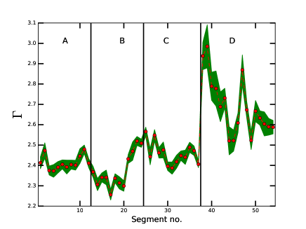
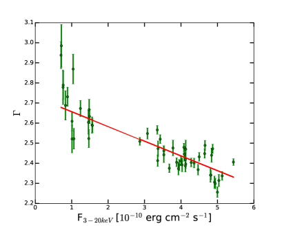
Figure 5: Variation of $\Gamma_{\rm PL}$ with segment number (left panel). The green shaded band is the one $\sigma$ error region and the black lines show the transition from one observation to the other. The right panel shows the $\Gamma_{\rm PL}$ variation with total flux. The red solid line is the weighted linear least square fit to the data. Both panels show a significant change in $\Gamma_{\rm PL}$ from 2.2 to 3.0 in about 83 days.

Table 4: Best fitting parameters and fluxes for the models tbabs*pl to NuSTAR. Here, flux is in $10^{-10}$ erg cm²sec^-1 unit.

Epoch	MJDstart	MJDend	$\Gamma_{\rm PL}$	$F_{\rm 3-60keV}$	$\chi_{r}^{2}/dof$
A	57756.99385	57757.52163	$2.436\pm 0.006$	$5.166\pm 0.017$	1.2/456
B	57784.99038	57785.55288	$2.421\pm 0.006$	$5.547\pm 0.006$	1.4/452
C	57812.92441	57813.49733	$2.488\pm 0.006$	$5.335\pm 0.022$	1.5/451
D	57839.91052	57840.63969	$2.661\pm 0.011$	$1.430\pm 0.001$	1.0/316

Table 5: Parameters of tbabs*zxipcf*thcomp*diskbb model fits to the spectra. Here, $C_{\rm f}$ is the partial covering fraction, $kT_{e}$, and $\Gamma$ are the temperature of the corona and photon index of the spectrum respectively. $T_{\rm in}$ and N_dbb are the temperature and normalization of the diskbb model component.

Epoch	MJDstart	MJDend	$C_{\rm f}$	$kTe$	$\Gamma$	$T_{\rm in}$	Ndbb	$\chi_{r}^{2}/dof$
				[keV]		[keV]	$\times 10^{13}$
A	57756.99385	57757.52163	$0.26\pm 0.02$	$144\pm 46$	$2.49\pm 0.06$	$0.07\pm 0.02$	$3.13\pm 1.02$	1.0/451
B	57784.99038	57785.55288	$0.33\pm 0.07$	$55\pm 8$	$2.53\pm 0.09$	$0.08\pm 0.02$	$0.61\pm 0.17$	0.9/448
C	57812.92441	57813.49733	$0.3\pm 0.03$	$51\pm 9$	$2.6\pm 0.1$	$0.08\pm 0.02$	$0.26\pm 0.05$	1.1/446
D	57839.91052	57840.63969	$0.07\pm 0.01$	$27\pm 5$	$2.58\pm 0.07$	$0.09\pm 0.02$	2.9e$-$3$\pm$3e$-$4	1.0/312

Table 6: Results of tbabs*zxipcf*tcaf model fits to the spectra. $\dot{m}_{\rm d}$, and $\dot{m}_{\rm h}$ represent tcaf model fitted sub-Keplerian (halo) and Keplerian (disc) rates in Eddington rate unit respectively. $X_{s}$ (in Schwarzchild radius $r_{s}$), and $R$ are the model fitted shock location and shock compression ratio values respectively. $N_{t}$ is the model normalization. Fluxes are in $10^{-10}$ ergs cm^-2 s^-1.

MJDstart	MJDend	$C_{\rm f}$	$\dot{m}_{\rm d}$	$\dot{m}_{\rm h}$	$X_{\rm s}$	R	$N_{t}\times 10^{4}$	$F_{\rm tot}$	$F_{\rm disk}$	$F_{\rm jet}$	$\chi_{r}^{2}$
57756.99385	57757.52163	$0.31\pm 0.03$	$0.021\pm 0.002$	$0.221\pm 0.011$	$19.77\pm 3.79$	$1.91\pm 0.31$	$1.36\pm 0.18$	$5.09\pm 0.02$	$1.61\pm 0.01$	$3.48\pm 0.02$	1.0/450
57784.99038	57785.55288	$0.36\pm 0.04$	$0.028\pm 0.002$	$0.232\pm 0.012$	$9.80\pm 1.61$	$2.42\pm 0.53$	$2.02\pm 0.31$	$5.30\pm 0.01$	$1.25\pm 0.01$	$4.05\pm 0.01$	0.9/447
57812.92441	57813.49733	$0.24\pm 0.03$	$0.035\pm 0.003$	$0.278\pm 0.045$	$10.81\pm 2.02$	$2.23\pm 0.32$	$1.35\pm 0.22$	$5.16\pm 0.02$	$1.71\pm 0.01$	$3.44\pm 0.03$	1.1/446
57839.91052	57840.63969	$0.06\pm 0.01$	$0.051\pm 0.013$	$0.346\pm 0.031$	$9.90\pm 1.68$	$1.72\pm 0.13$	$0.42\pm 0.03$	$1.41\pm 0.01$	$1.41\pm 0.01$	$-$	1.0/311

3.3 X-ray variability

To quantify the X-ray flux variation, we used the excess variance or the fractional variability amplitude $F_{\rm{var}}$ (Edelson et al., 1996; Nandra et al., 1997; Vaughan et al., 2003). $F_{\rm{var}}$ is the variance after subtracting the contribution expected from measurement errors and is defined as

$$\centering{}F_{\rm{var}}=\sqrt{{S^{2}-{\bar{\sigma^{2}}_{\rm{err}}}\over\bar{x}^{2}}}\@add@centering$$ (1)

where ${\bar{x}^{2}}=\sum_{i=1}^{N}{x_{i}/N}$ is the arithmetic mean of $x_{i}$. ${S^{2}}$ and $\overline{\sigma_{\rm err}^{2}}$ are the sample variance of the light curve and mean square error associated with the measured fluxes $x_{i}$ respectively.

$$\centering S^{2}=\frac{1}{N-1}\sum_{i=1}^{N}(x_{i}-\bar{x})^{2},\@add@centering$$ (2)

$$\overline{\sigma_{\rm err}^{2}}=\frac{1}{N}\sum_{i=1}^{N}\sigma^{2}_{\rm{err,i}}$$ (3)

Using Eq. (1), we calculated the fractional variability amplitude for each segment of observations and the measurement uncertainties of $F_{\rm{var}}$ were estimated following Vaughan et al. (2003)

$$\centering{}\text{err}(F_{\rm{var}})=\sqrt{\Bigg{(}\sqrt{1\over{2N}}{\overline{\sigma_{\rm err}^{2}}\over{{\bar{x}}^{2}}{F_{\rm{var}}}}\Bigg{)}^{2}+\Bigg{(}\sqrt{\overline{\sigma_{\rm err}^{2}}\over{N}}{1\over\bar{x}}\Bigg{)}^{2}}\@add@centering$$ (4)

The results of the variability analysis are listed in Table 7. We found the amplitude of the flux variations to increase from epoch A to epoch D and the highest flux variations were seen in epoch D.

Table 7: Flux variability characteristics for each epoch of Mrk 421.

OBS ID	Epoch	$F_{\rm{var}}\pm\text{err}(F_{\rm{var}})$
		3$-$10 keV	10$-$20 keV	3$-$20 keV
60202048002	A	0.079$\pm$0.001	0.085$\pm$0.002	0.080$\pm$0.001
60202048004	B	0.139$\pm$0.001	0.203$\pm$0.002	0.156$\pm$0.001
60202048006	C	0.163$\pm$0.001	0.187$\pm$0.001	0.168$\pm$0.001
60202048008	D	0.272$\pm$0.001	0.353$\pm$0.002	0.276$\pm$0.021

In the observed period presented here, the hardness ratio (HR) was calculated for each segment from the pl model fitted spectra for the energy range 3$-$20 keV. In our case $HR=\frac{F_{10-20keV}}{F_{3-10keV}}$, where, $F_{10-20keV}$ and $F_{3-10keV}$ are the flux in hard and soft energy bands. In Figure 6, we show the HR variation with total observed flux. In $\sim$83 days, HR changed by a factor of more than 2, and during the fourth epoch (2017 March 27), the source had the lowest hard flux. We performed the weighted least square fitting to the observed data points in the HR v/s flux diagram. We found a strong positive correlation between the HR and total flux. We obtained a correlation coefficient of 0.874 which also indicates that our spectrum become harder as the flux increases, confirming the results which are interpreted from photon index vs. flux diagram (Figure 5). It can also be seen from Table 3 that there is a noticeable transition in flux in all energy bands. Between epoch C and epoch D the brightness in the soft band reduced by a factor of 7 in magnitude, whereas in the hard band the brightness dropped by a factor of 12. This large jump in flux between epoch C and D also implies that the corona which reprocesses soft photons from the Keplerian disc and scatters them as hard radiation has significantly cooled down, therefore can not produce enough hard radiation, and the source moved to lower flux state. This abrupt change in the flux is a signature of (a) sudden change in flow configuration, which means viscosity has changed suddenly (Mondal et al., 2017) or (b) appearance of some absorbers. The significant change in CENBOL geometry consistent with the flux variation can also be seen from the tcaf model fitted parameters, where the size of the CENBOL has changed by a factor of $\sim 2$. Also, this is consistent with the estimated decrease in the temperature of the corona from epochs A to D. From Table 7, it is evident that hard X-rays are more variable than the soft X-rays. This might be indicative of more complex dependence of variability on energy and other physical mechanisms. The difference between soft and hard X-ray variability could be, for example, related to the size of the emitting region, or the corona and thus the cooling effect. There are arguments in the literature on the similar observational flux variability characteristics noticed here. If the high-energy electron cloud is located at the inner edge of the accretion disc, which is the Comptonizing corona in our case or above its inner part (Zdziarski et al., 1999), and the low-energy emitting region is associated to some outflow from the disc or a second cloud with lower temperature (Petrucci et al., 2013), then the hard flux could be more variable than the soft flux. This could explain both the harder when brighter trend in the spectra and the hotter when brighter trend in the corona of Mrk 421.

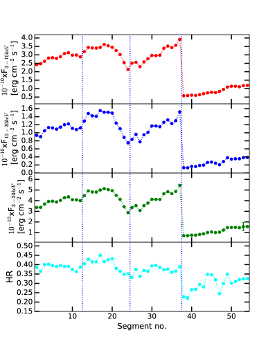
Figure 6: Variation of the soft (3$-$10 keV), hard (10$-$20 keV) and total (3$-$20 keV) fluxes and hardness ratio (HR).

3.4 Contribution of the jet to spectral flux

In this section, we compare the spectral fitting with the accretion disc model to estimate the contribution from both disc and jet. To investigate the relative importance of jet emission over the accretion disc emission in Mrk 421 as well as to compare the parameters obtained from spectral fits to the data acquired during 2017, we identified one NuSTAR data (OBSID = 60002023031, hereinafter Epoch E) observed on 14 April 2013. The source was in a very active state in $\gamma$-rays, optical and X-rays during epoch E, and the X-ray emission during this epoch is expected to be dominated by the emission from the relativistic jet. The R-band, the Swift/XRT soft and hard bands, and UV fluxes are $11.90\pm 0.03$ (mag), $77.41\pm 0.26$, $50.62\pm 0.18$, and $30.97\pm 0.74$ in ph s^-1 unit respectively. The hardness ratio (hard/soft flux) was 0.65 during this epoch. We fitted the spectra obtained during Epoch E, with pl, thcomp and tcaf. The pl was not found to be useful, and indeed, returned a poor fit with $\chi_{r}^{2}$ of 3.7 during epoch E, while tcaf fits well ($\chi_{r}^{2}$ of 1.18) the data with $\dot{m}_{d}=0.43$, $\dot{m}_{h}=0.304$, $X_{s}=27.47$, and $R=2.82$. The normalization from tcaf fit was found to increase by a factor of about 60 times, compared to the normalization obtained during epoch D, when the source was in the lowest flux state in X-rays among all the epochs analysed here. The total X-ray flux was also high with the value $27.57\times 10^{-10}$ ergs cm^-2 s^-1. In Figure 7 we show the tcaf model fitted spectrum when the normalization is free (in panel a) and for an average normalization (in panel b) obtained from the fit of other epochs. The panel (b) does not fit the data very well when the normalization for the fit is frozen to the average value obtained from the relatively low flux data (epochs A-D) fitting. Moreover, it shows that the spectrum is softening gradually, this can be due to the cooling effect in jet and can be well explained by the logpar model, often used for this source. Therefore, our comparative fitting of the less and very active jet epochs shows that the disc could be present, however, might be weak and subdominant. We also point out that multi-band data from UV/optical, X-ray, and $\gamma$ gathered during the same epochs analysed in this work was equally fit with synchrotron and SCC models (MAGIC Collaboration et al., 2021). It is to be noted that for moderately emitting X-ray jets, tcaf is enough to fit, since tcaf uses cylindrical geometry for interception flux calculations. For computation of average optical depth, tcaf code does not use a slab geometry given in Sunyaev & Titarchuk (1980) rather it uses a spherical geometry. In both the cases, the centrifugal force supported torus and matter inside the funnel of the torus which constitutes the pre-jet matter till the sonic surface) were taken care of while computing the intercepted photons. For consistency, we checked that the thcomp also fits the data well with $kT_{\rm e}=24\pm 6$ keV and $\Gamma=2.41\pm 0.05$.

As the normalization is a scale factor which depends on the source distance and its inclination, therefore it is constant between epochs for a particular source. If its value changes drastically, this could point to an additional emission process contributing to the observed X-ray, for example, emission from the jet. Therefore, the normalization can also be a probe to estimate the flux contributions from both the disc and jet. This has been successfully applied to black hole binary systems (Jana et al., 2017, and others). As Mrk 421 is a jetted candidate, we applied that finding for this candidate as a case study. Considering that in the lowest normalization epoch, the flux contribution is mainly from the disc, and increasing norm implies an excess contribution from the jet in addition to the disc contribution. Therefore, the total flux $F_{\rm total}$ can be written as the sum of disc and jet, as below:

$$F_{\rm total}=F_{\rm disk}+F_{\rm jet}.$$ (5)

Here, $F_{\rm disk}$ can be obtained by using the lowest norm in epoch D to all other epochs and the jet contribution can be estimated by subtracting the lowest flux contribution from the disc from the total flux in Table 6 (in Column 8 when the norm is free). Therefore, for this epoch, F_jet is zero. This is also reflected in the third panel of Figure 8.

For all the epochs, we show in Figure 8 the relation ($ax^{b}$) between the radio flux (a proxy for jet emission) against the X-ray emission coming from different components of the accretion-jet system. The three panels in Figure 8 show the variation of the radio flux with the total flux, disc flux from tcaf fits and the jet flux obtained from Equation 5. In this figure, the red circles are the observed/estimated flux values, while the solid black curve is the fitted function. We find that the radio flux is anti-correlated with the X-ray flux from the accretion disc, while it is correlated with the jet X-ray emission. The normalization in tcaf fits increases from Epochs D $\rightarrow$ C $\rightarrow$ A $\rightarrow$ B $\rightarrow$ E. This indicates that the relative contribution of the jet emission over the disc emission increases in the sequence D$\rightarrow$C$\rightarrow$A$\rightarrow$B$\rightarrow$E, with the X-ray jet emission being maximum during epoch E and minimum during epoch D.

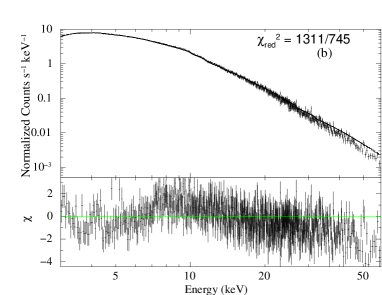
Figure 7: The 3$-$60 keV spectra fitted with tbabs*zxipcf*tcaf model along with the residuals for epoch E. The panels (a) shows the fit when tcaf model norm is free and (b) corresponds to data fitted when norm is frozen to an average low flux state norm around 1.3e4.

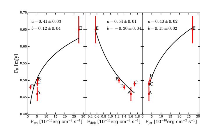
Figure 8: Radio flux variation with different components of the flux obtained from tcaf model fit. The red solid circles are the observed data points and the black solid line is the functional dependence between fluxes.

3.5 Joint fit to the Swift/XRT and NuSTAR data

For estimating various accretion parameters as discussed in the previous section, we used only data from NuSTAR covering the energy range from 3-60 keV. It is likely, that inclusion of X-ray data with energies lower than 3 keV could have an impact on the derived accretion parameters. To test this, we did a joint spectral analysis of Swift/XRT and NuSTAR data with thcomp and tcaf models.

For Swift/XRT data, the spectrum files were generated using the online product generator (Evans et al., 2009). The data were binned to 20 counts rate per energy bin. For the joint spectral analysis, we used data in the energy range from 0.4 to 60 keV. For epochs A to D, Swift/XRT data covering the energy range of 0.4 to 8 keV was used except for epoch C, where the data from energy range 0.4 to 5 keV was used, owing to poor S/N beyond 5 keV. The results of the thcomp model fit to the joint Swift/XRT and NuSTAR data are given in Table 8. A comparison of Table 8 with that of Table 5 indicates the parameters obtained from combined Swift/XRT + NuSTAR data and NuSTAR data alone agree within errors. Similarly, we show in Figure 9, the tcaf model fits to the combined spectra, and the derived parameters are given in Table 9. In tcaf model fits too, the parameters obtained from the joint Swift/XRT and NuSTAR data agree within errors to the parameters obtained using only NuSTAR data. In model fits to the combined data set, an extra Gaussian component was required to fit the excess flux in the 0.5 - 0.7 keV range. We note that the disc parameters (that are needed for the estimation of viscosity parameter) obtained from joint fitting are in agreement to that obtained using NuSTAR data alone within errors.

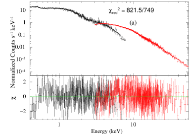
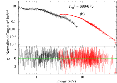
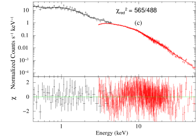
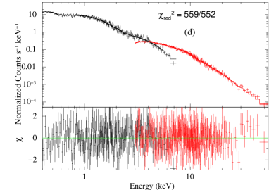
Figure 9: The 0.4$-$60 keV combined Swift/XRT and NuSTAR spectra fitted with tbabs*zxipcf*(tcaf+gauss) model along with the residuals. The panels (a)-(d) correspond to the data acquired at epochs A, B, C and D respectively.

Table 8: Results of tbabs*zxipcf*thcomp*(diskbb+gauss) model fits to the joint Swift/XRT and NuSTAR spectra. The gauss component is required at $\sim 0.5-0.7$ keV energy range to fit the excess around that energy. The other parameters are the same as in Table 5.

Epoch	MJDstart	MJDend	$C_{\rm f}$	$kTe$	$\Gamma$	$T_{\rm in}$	Ndbb	$\chi_{r}^{2}/dof$
				[keV]		[keV]	$\times 10^{6}$
A	57756.99385	57757.52163	$0.57\pm 0.11$	$138\pm 12$	$2.40\pm 0.01$	$0.07\pm 0.01$	$4.07\pm 0.39$	1.0/750
B	57784.99038	57785.55288	$0.63\pm 0.03$	$35\pm 4$	$2.43\pm 0.02$	$0.07\pm 0.02$	$4.62\pm 0.25$	1.0/676
C	57812.92441	57813.49733	$0.65\pm 0.08$	$38\pm 5$	$2.48\pm 0.03$	$0.07\pm 0.02$	$3.91\pm 0.40$	1.1/489
D	57839.91052	57840.63969	$0.12\pm 0.01$	$21\pm 3$	$2.54\pm 0.04$	$0.07\pm 0.01$	$1.32\pm 0.11$	1.1/553

Table 9: Results of tbabs*zxipcf*(tcaf+gauss) model fits to the joint Swift/XRT and NuSTAR spectra. The gauss component is required at $\sim 0.5-0.7$ keV energy range to fit the excess around that energy. The other parameters are the same as in Table 6.

MJDstart	MJDend	$C_{\rm f}$	$\dot{m}_{\rm d}$	$\dot{m}_{\rm h}$	$X_{\rm s}$	R	$N_{t}\times 10^{4}$	$F_{\rm tot}$	$F_{\rm disk}$	$F_{\rm jet}$	$\chi_{r}^{2}/dof$
57756.99385	57757.52163	$0.48\pm 0.03$	$0.022\pm 0.003$	$0.222\pm 0.010$	$20.09\pm 2.48$	$2.41\pm 0.36$	$0.99\pm 0.13$	$14.23\pm 0.04$	$5.42\pm 0.02$	$8.81\pm 0.05$	1.49/749
57784.99038	57785.55288	$0.77\pm 0.13$	$0.027\pm 0.001$	$0.243\pm 0.011$	$9.91\pm 1.23$	$2.38\pm 0.34$	$0.93\pm 0.15$	$14.23\pm 0.04$	$7.05\pm 0.05$	$7.19\pm 0.06$	1.0/675
57812.92441	57813.49733	$0.78\pm 0.16$	$0.034\pm 0.004$	$0.292\pm 0.011$	$10.98\pm 2.59$	$2.87\pm 0.21$	$1.05\pm 0.24$	$16.72\pm 0.42$	$5.00\pm 0.01$	$11.73\pm 0.30$	1.15/488
57839.91052	57840.63969	$0.46\pm 0.02$	$0.051\pm 0.008$	$0.348\pm 0.021$	$9.93\pm 1.63$	$1.73\pm 0.19$	$0.26\pm 0.04$	$5.95\pm 0.08$	$5.95\pm 0.08$	–	1.0/552

3.6 Estimating accretion disc viscosity parameter

Flux variability of different time scales (hours to years) in AGN can be explained by several theoretical models (a) relativistic jet based models (Marscher & Gear, 1985; Gopal-Krishna & Wiita, 1992; Calafut & Wiita, 2015) where the variability time scale is large and (b) the accretion disc based models where the variability can be in small scales. In case of the later models, it is believed that the observed X-ray variability in both black hole X-ray binaries and Seyfert galaxies mainly comes from two key components, accretion disc and its dynamic corona where the X-rays are predominantly produced close to the BH by IC scattering of the optical/UV seed photons from the accretion disc. On the other hand, the geometrically thin, cold, and optically thick accretion disc reprocesses the variable X-ray emission coming from the innermost optically thin, hot corona in a complex way, therefore playing mostly a passive role in the variability at the shortest timescales. Furthermore, it has been interpreted by studying different timescales in accretion disc of blazars that the observed variations are solely due to jet or by the variations in the disc carried out, and amplified by jets (Wiita, 2006). Hence, the X-ray variability can be used to probe the properties of accretion on to the BH. The physical scenarios that describe the large scale variability in different accretion disc based models are the formation and fragmentation of spiral shocks in accretion disc (Wiita et al., 1992; Chakrabarti & Wiita, 1993), the asymmetries and geometric effects in accretion disc (Mangalam & Wiita, 1993), or by the fluctuations that propagate from the outer radii of the accretion disc towards the center and couple with the emission from the inner region of the disc (Lyubarskii, 1997; Arévalo & Uttley, 2006). It has been shown for black hole X-ray binaries that the viscosity and inverse Compton cooling can be responsible for small scale variability and different flux states (Mondal et al., 2017) during the outburst phase of the BHs. The timescales of these variations can be scaled up for AGN through the BH mass (McHardy et al., 2006).

Studying the variability using any physical accretion disc model is important to understand the underlying dynamics behind these. X-ray flux variations in blazars in the low flux state can possibly be explained by disc accretion. Very recently, Chatterjee et al. (2018) discussed on the accretion disc origin of variability of Mrk 421 using AstroSat data. Here, we use the results of the spectral analysis of the X-ray observations of Mrk 421 by NuSTAR during 2017 using tcaf model to understand the flux variations possibly being caused by accretion disc through the accretion rate variation, which also represents the viscosity ($\alpha$) fluctuation.

It is believed that $\alpha$ parameterization provides the basis for developing the accretion disc theory and related observations. There are several methods to estimate $\alpha$ parameter. For instance, in the case of observations, if we assume that the optical variability of the AGN is caused by disc instabilities, then comparing the thermal timescales of $\alpha$-disc (Shakura & Sunyaev, 1973, hereafter SS73) models with the observed variability timescales, one can put constraints on the viscosity parameter for different candidates (Siemiginowska & Czerny, 1989; Starling et al., 2004). In the numerical simulation, Balbus & Hawley (1991) showed that $\alpha$-parameter can be obtained from the outward transport of angular momentum in weakly magnetized disc by magnetohydrodynamic turbulence. Pessah et al. (2007) inferred observationally that in order to make MRI-driven turbulence, the angular momentum transport is required for large values of the effective $\alpha$ viscosity ($\alpha\geq 0.1$), the disc must be threaded by a significant vertical magnetic field and the turbulent magnetic energy must be in near equipartition with the thermal energy. On the other hand, in an advection-dominated disc, Narayan & McClintock (2008) argued that the required viscosity is 0.1$-$0.3. All these estimates seem to show a very broad range of the $\alpha$ parameter, 0.001$-$0.6 (see also Hawley et al., 1995). However, a narrow range of $\alpha$ parameter for blazars has been estimated by Xie et al. (2009). In this work, we made an attempt to estimate the viscosity parameter for Mrk 421.

To estimate the viscosity parameter we used the disc accretion rate returned by tcaf model fits to the spectra. We assumed that the disc radiates locally as a black body with an effective temperature,

$$T=\left(\frac{3GM_{\rm BH}\dot{M}}{8\pi\sigma}\right)^{1/4}f^{1/4}r^{-3/4},$$

where $f=[1-(r_{\rm in}/r)^{1/2}]\sim 1$, $r$ is the radial distance of the disc. We considered the outer boundary of the disc as 500 $r_{s}$. The kinematic viscosity $(\nu)$ can be written as

$$\nu=\frac{\dot{M}}{3\pi\Sigma},$$

where, $\Sigma$ is the surface density of the disc and can be obtained from the density ($\rho$ in gm cm^-3) and scale height ($H$ in cm) of the disc. According to SS73 prescription, $\nu$ can be written as $\alpha c_{s}H$, where $c_{s}$ is the isothermal sound speed, corresponding to the effective disc temperature. After combining these equations and performing a few steps of algebra, we obtained the $\alpha$-parameter value. Our estimated values of $\alpha$ ranges between 0.18$-$0.25 in the Keplerian component of the two component disc. We also estimated different time scales of the flow, for example the dynamical ($t_{\rm dyn}=\sqrt{GM_{\rm BH}/r^{3}}$) and thermal time scales ($t_{\rm th}=\alpha^{-1}t_{\rm dyn}$) are $\sim$ 2 years and 8$-$10 years respectively, whereas the viscous timescale ($t_{\rm vis}=t_{\rm th}(H/r)^{2}$) is $\sim$ 30$-$36 Myr.

4 Conclusions

In this paper, we studied the flux and spectral variability of Mrk 421 using NuSTAR data obtained in 2017 and in 2013. During the 2017 epoch, we found the pl photon index to change from 2.2 to 3.0. We split each epoch of observation into several segments to study the flux and spectral variability on short time scales. We noticed that while the hardness ratio (Table 3) is almost doubled, the average count rate of the source varied by a factor of 4 in $\sim 83$ days. We found that each epoch of observation in the energy band 3$-$60 keV could be well fitted with phenomenological thcomp and physical tcaf models. Each segment of data could be well fitted with the simple pl model. From the obtained $F_{\rm var}$ (in Table 7), we conclude that the source was significantly variable in all the epochs. We also found a strong correlation between the pl index and the brightness of the source in the total energy band with a “harder when brighter” behaviour.

Mrk 421 is a HSP blazar which generally lacks emission lines in the optical spectra. Under such circumstances, the origin of the observed X-ray flux variations lie in their jets (Abdo et al., 2011). Alternatively, during the less active state, one may expect the contribution of accretion disc to the observed emission, however, unlikely to dominate over jet contribution. Recently, Chatterjee et al. (2018) noticed a break in the power spectral density from X-ray observations of Mrk 421 at around the same time as that of the NuSTAR data which is analysed here. The observations from AstroSat used by Chatterjee et al. (2018) were also taken during the moderate brightness state of Mrk 421. Such breaks, that are normally seen in the X-ray power spectral density of Seyfert galaxies, are believed to be due to the X-ray being produced in the accretion disc. We therefore, hypothesise that in the low or moderate X-ray activity of Mrk 421, disc emission could manifest itself in the observed X-rays and thus fit each epoch of data using the disc-based tcaf model to investigate if the observed flux variations can be explained with changes in the accretion rate or changes in the geometry of the accretion disc. The derived parameters from the model fits show that the disc mass accretion rate has varied by a factor of $\sim$3 from $0.02$ to $0.051$ $\dot{M}_{\rm Edd}$ and the size of the CENBOL as envisaged in tcaf model also changed significantly. This size varied from 20 to 10 $r_{s}$ between epochs A and D. In epoch D, the inner edge of the disc moved significantly inward with the lowest shock compression ratio and the shrinking of the CENBOL was maximum, and the accretion rate was the highest. This implies a transition of the source to a lower flux state with a significant flux change. Also, the temperature of the CENBOL was found to change from epoch A to D, using both physical tcaf and phenomenological thcomp model fits. The CENBOL was found to be hotter with increasing brightness of the source. Therefore, the shrinking of the CENBOL, increase of the mass accretion rates, and the decrease in the flux values follow the correlation with $\Gamma_{\rm PL}$ variation. Even though both the model temperatures are showing the same profile, the static corona (used in thcomp) cannot behave in the same way as the dynamic corona/CENBOL (used in tcaf) does because the static corona would cool quickly if there is no underlying heating mechanism. Therefore, the temperature estimated from tcaf model is more realistic.

We note that the accretion disc-based model like tcaf can fit the spectra without adding any other component. This indicates that even though Mrk 421 is a HSP blazar, in the low/moderate activity state during the period of our observation, the disc could contribute significantly to the total observed X-ray emission, however, not dominating over the jet contribution. The difference in the flux variations between the hard and soft bands and subsequently the hardness ratio could also be due to changes in the size of the emission region or the CENBOL. Thus, the hard emission might have its origin from the changing corona region at the inner edge of the disc. On the other hand, the presence of jet and its contribution to the total spectra would imply that the gravitational potential energy of the infalling matter not only gets transformed into radiation, but can also amplify magnetic field, that allows the field to retrieve large store of rotational energy and transform a part of it to jet power.

Thus, based on the modelling of the five epochs of NuSTAR data of Mrk 421 for the energy band 3-60 keV from the relatively less and very high jet activity, we conclude that (i) simple pl alone is not a good representation of the observed X-ray rather cutoffpl fits the data well, (ii) both tcaf and thcomp fit the observed X-ray emission well to give the accretion and spectral properties though tcaf gives the physical parameters of the flow, (iii) non-magnetic accretion disc models are found to be adequate to fit the low/moderate X-ray activity state data of Mrk 421. However, the X-ray/$\gamma$-ray correlation is one of the important characteristics in the broadband emission of Mrk 421, that occurs during high and low activity, as reported multiple times in the literature over the last years, and particularly for the data obtained in the year 2017, as reported in MAGIC Collaboration et al. (2021). The existence of this correlation implies a substantial emission from the jet, probably related to SSC models, that occurs also during the very low activity. And hence that, even during the low blazar activity, the present disc-base models can not dominate the X-ray emission of Mrk 421.