Abstract

Witten diagrams provide a perturbative framework for calculations in Anti-de-Sitter space and play an essential role in a variety of holographic computations. In the case of this study in AdS₂, the one-dimensional boundary allows for a simple setup, in which we obtain perturbative analytic results for correlators with the residue theorem. This elementary method is used to find all scalar $n$-point contact Witten diagrams for external operators of conformal dimensions $\Delta=1$ and $\Delta=2$, and to determine topological correlators of Yang-Mills in AdS₂. Another established method is applied to explicitly compute exchange diagrams and give an example of a Polyakov block in $d=1$. We also check perturbatively a recently proposed multipoint Ward identity with the strong coupling expansion of the six-point function of operators inserted on the 1/2 BPS Wilson line in $\mathcal{N}$=4 SYM.

HU-EP-22/14-RTG

1 Discussion

The two-dimensional Anti-de-Sitter space AdS₂ provides a wonderful playground both to study quantum field theory in curved space and to further our understanding of correlation functions in AdS/CFT. As there are no propagating degrees of freedom for the graviton, the latter is not a usual gauge/gravity correspondence, but rather a rigid holography that has physical settings e.g. in the context of defects in higher-dimensional theories [1, 2, 3, 4, 5, 6], effective and intrinsic theories in AdS₂ [7, 8, 9, 10, 11, 12, 13, 14, 15, 16, 17, 18]. Perturbative computations in Anti-de-Sitter space are done through Witten diagrams, whose structure has extensively been studied [19, 20, 21, 22, 23, 24, 25, 26, 27, 28, 29]. Yet, the complexity relative to their flat space counterpart is still a roadblock to perturbative analysis and there is still a search for the full equivalent of Feynman rules [30]. As such, the most efficient methods to date for perturbative correlators are through the conformal bootstrap [31, 32]. However, explicit computations remain a reliable way to make progress in perturbation theory and can provide some insight into assumptions that may simplify the bootstrap process. First-order four-point correlators with quartic interactions in the strong coupling limit can be written in terms of $D$-functions [21] which are four-point Witten contact diagrams. At higher order, with loops and exchanges which correspond to additional integrated bulk points, some diagrams can be related to contact integrals through differential equations [22, 33]. As such, the $n$-point $D$-functions are used beyond the first order and can be seen as a starting point to build ‘master integrals’ for Witten diagrams. AdS₂ is a perfect place to look at these integrals as it provides a simple framework with relevance in its own right (e.g. in defect theories) and corresponds to a diagonal limit ($z=\bar{z}$ for four points) of its higher-dimensional counterparts.

Boundary correlators in AdS₂ enjoy a one-dimensional conformal symmetry. In higher dimensions, along with additional symmetries, this simplifies perturbative computations. However, the structure of AdS₂ provides a framework in which another elementary method can be used to compute perturbative quantities; the residue theorem. Using contour integration for one of the AdS₂ integrals, the contact diagram in $\lambda_{n}\phi_{\Delta}^{n}$ theory for $n$ scalars of low conformal dimension is remarkably simple leading to the results (see Section 3 below)

$$I_{\Delta=1,n}(x_{i}) =\frac{\pi}{(2i)^{n-2}}\sum_{i\neq j}\frac{x_{ij}^{n-4}}{\Pi_{k\neq i,j}x_{ik}x_{jk}}\log\left(\frac{x_{ij}}{2i}\right),$$ (1.1)

$$I_{\Delta=2,n}(x_{i}) =\sum_{j\neq i}\frac{-\pi}{2(2i)^{2n-4}x_{ij}^{2}}\partial_{x_{i}}\left(\frac{x_{ij}^{2n-5}}{\prod_{k\neq i,j}x_{ik}^{2}x_{jk}^{2}}\log\frac{x_{ij}}{2i}\right)$$ (1.2)

$$+\sum_{j\neq i}\partial_{x_{j}}\frac{-\pi}{(2i)^{2n-2}x_{ij}^{2}}\partial_{x_{i}}\left(\frac{x_{ij}^{2n-4}}{\prod_{k\neq i,j}x_{ik}^{2}x_{jk}^{2}}\log\frac{x_{ij}}{2i}\right).$$

Above, $I_{\Delta,n}(x_{i})$ is the integral corresponding to the Witten contact diagram of $n$ fields $\phi_{\Delta}$ of conformal dimension $\Delta$ inserted at positions $x_{i}$, where $x_{ij}=x_{i}-x_{j}$ throughout the text. Here, the normalisation of the propagator is set to one. For the canonical normalisation, one can simply multiply by the quantity defined in (2.22) for each propagator. These expressions are in terms of the operators’ positions and combine naturally into the cross-ratios obtained with the usual conformal transformations (see discussion in Section 2.1 around equation (2.5) and Appendix A.2). This method proves to be even more powerful in some settings where the residue theorem can be used for both of the bulk coordinates. This is the case for the topological three-point correlator of the boundary fields $a$ of the gauge field of pure Yang-Mills in AdS₂ presented in [34], providing an alternative derivation in Section 4 of

$$\langle a^{a}(x_{1})a^{b}(x_{2})a^{c}(x_{3})\rangle=-\frac{1}{4\pi g_{YM}^{2}}f^{abc}\textrm{sgn}(x_{12}x_{23}x_{31}),$$ (1.3)

where $f^{abc}$ are the structure constants of the gauge group of the Yang-Mills theory. The low dimensionality has other advantages, such as having fewer cross-ratios. For four-point functions, for example, the single cross-ratio simplifies the differential equation used to compute exchange diagrams in Section 5. We thus compute explicitly a Polyakov block corresponding to the sum of four-point exchange Witten diagrams with dimensions $\Delta=1$, which agrees with independently found results

$$P_{1,1}^{(0)}(\chi) =\text{Li}_{2}\left(\frac{\chi}{\chi-1}\right)\log\left(\frac{\chi^{2}}{(\chi-1)^{2}}\right)-6\text{Li}_{3}\left(\frac{\chi}{\chi-1}\right)-\frac{1}{6}\pi^{2}\log\left(\frac{\chi^{2}}{(\chi-1)^{2}}\right)+6\zeta(3)$$

$$+\frac{\text{Li}_{2}(1-\chi)\log\left((\chi-1)^{2}\right)-6\text{Li}_{3}(1-\chi)-\frac{1}{6}\pi^{2}\log\left((\chi-1)^{2}\right)+6\zeta(3)}{\chi^{2}}$$

$$+\frac{\text{Li}_{2}(\chi)\log\left(\chi^{2}\right)-6\text{Li}_{3}(\chi)-\frac{1}{6}\pi^{2}\log\left(\chi^{2}\right)+6\zeta(3)}{(\chi-1)^{2}},$$ (1.4)

where $\chi=\frac{x_{12}x_{34}}{x_{13}x_{24}}$ is the four-point function cross-ratio. Natural extensions to this work include deriving position space results of contact diagrams in the case of higher external dimensions and Polyakov blocks for higher exchanged dimensions. A possible path for this is by extending the one-dimensional Mellin analysis developed in [35] to higher $n$-point functions using results from this study. In the former, Mellin amplitudes for higher $\Delta$ were obtained, so that, in combination with these notes, results for all $(n,\Delta)$ may be achievable. The knowledge of the structure of contact diagrams also sheds light on the computation of higher-point exchange diagrams through the method presented in Section 5. A combination of these two techniques for contact and exchange diagrams could also, along with multipoint Ward identities and bootstrap methods, provide a path to the computation of the strong coupling, second-order, 6-point correlator of the 1/2-BPS defect in $\mathcal{N}=4$ SYM. In this spirit, an appendix is included providing a perturbative check of the consistency of the multipoint Ward identities conjectured in [36] for the first two strong coupling perturbative orders of the 6-point correlator of insertions on the 1/2 BPS line in $\mathcal{N}=4$ SYM. The higher-order quantities are beyond the scope of this paper and are left for further investigation.

The paper will proceed as follows; after an introduction to the basics, techniques, and notations of CFT₁ and AdS₂ in Section 2, contour integration will be used in Section 3 to derive the AdS₂ massless $n$-point contact diagrams which are consistent with the numerical integration and the current literature. This method will also be used in Section 4 to derive the topological three-point correlator of the boundary field of pure Yang-Mills in AdS₂. Finally, known methods will be applied in Section 5 to find the explicit expression of a one-dimensional Polyakov block, which has the correct symmetries, Regge behaviour, and double-discontinuity. Several technical appendices complete the manuscript.

2 Review of AdS₂/CFT₁ correlators

Interacting fields propagating in AdS₂ define a non-local one-dimensional conformal field at the boundary. We go through some basics of one-dimensional conformal theories, dynamics in two-dimensional Anti-de-Sitter space, and set up the notation of this paper. We also review the concepts of Polyakov blocks and the methods used in [26, 33] to relate AdS exchange diagrams to contact diagrams in the context of CFT₁.

2.1 CFT₁ basics, techniques, and notation

A one-dimensional conformal field theory can be defined by a set of data consisting of the spectrum $\{\Delta\}$ which defines which operators are present in the theory, and the coefficients $\{c_{\Delta_{1}\Delta_{2}\Delta_{3}}\}$ which define the interactions of these operators. Combined with the Operator Product Expansion (OPE), these can be used to reconstruct any correlator of local operators in the theory. The conformal group in $d=1$ is generated by the translation $P$, dilation $D$, and special conformal transformation $K$ which satisfy the conformal algebra and can be parametrised in one dimension by the differential operators

$$P =-\partial_{x} D =-x\partial_{x}-\Delta K =-x^{2}\partial_{x}-2\Delta x,$$ (2.1)

when acting on a field of conformal dimension $\Delta$ evaluated at position $x$. The consequence of these symmetries on correlators is that the coordinate dependence of the first three $n$-point correlators is fixed

$$\langle\phi_{\Delta}(x)\rangle=\delta_{\Delta,0}$$ (2.2)

$$\langle\phi_{\Delta_{1}}(x_{1})\phi_{\Delta_{2}}(x_{2})\rangle=\frac{\delta_{\Delta_{1},\Delta_{2}}}{x_{12}^{2\Delta}}$$ (2.3)

$$\langle\phi_{\Delta_{1}}(x_{1})\phi_{\Delta_{2}}(x_{2})\phi_{\Delta_{3}}(x_{3})\rangle=\frac{c_{\Delta_{1}\Delta_{2}\Delta_{3}}}{(x_{12})^{\Delta_{123}}(x_{13})^{\Delta_{132}}(x_{23})^{\Delta_{231}}}\qquad\quad\Delta_{ijk}=\Delta_{i}+\Delta_{j}-\Delta_{k}.$$ (2.4)

For $n$-point correlators, conformal transformations can be used to reduce the number of independent variables to $n\!-\!3$ conformally invariant cross-ratios

$$\chi_{i-1} =\frac{x_{1i}x_{n-1,n}}{x_{in}x_{1,n-1}} 0< \chi_{i}<1,$$ (2.5)

where $x_{ij}=x_{j}-x_{i}$ are real numbers in $d=1$. For equal conformal dimensions the correlator is

$$\langle\phi_{\Delta}(x_{1})..\phi_{\Delta}(x_{i})...\phi_{\Delta}(x_{n})\rangle=A(x_{1},...,x_{n})\langle\phi_{\Delta}(0)..\phi_{\Delta}(\chi_{i})...\phi_{\Delta}(1)\tilde{\phi}_{\Delta}(\infty)\rangle,$$ (2.7)

where

$$A(x_{1},...x_{n}) =\left(\left(\frac{x_{1n}x_{n-1,n}}{x_{1,n-1}}\right)^{n-2}\prod_{j=1}^{n-1}x_{jn}^{-2}\right)^{\Delta}.$$ (2.8)

One might wonder why higher-point correlators are of any interest since the theory can be determined by the set $\{\Delta,c_{\Delta_{1}\Delta_{2}\Delta_{3}}\}$. In practice, however, determining such a set is far from trivial, and working out perturbative higher-point correlators gives access to this information through the dynamics of the theory. For example, the four-point correlator has the following operator product expansion

$$<\phi_{\Delta}(x_{1})\phi_{\Delta}(x_{2})\phi_{\Delta}(x_{3})\phi_{\Delta}(x_{4})> =\frac{1}{(x_{13}x_{24})^{2\Delta}}f(\chi)$$ (2.9)

$$f(\chi) =\sum_{h}c^{2}_{\Delta\Delta h}\chi^{h-2\Delta}{}_{2}F_{1}(h,h,2h;\chi),$$ (2.10)

where $\chi=\frac{x_{12}x_{34}}{x_{13}x_{24}}$ is the usual cross-ratio ($\chi_{1}$ in (2.5)) for the four-point function in 1d. When computing the analytic expression of this four-point correlator at different orders in perturbation theory, for example using Witten diagrams in a holographic setup [1, 4], these can be equated to the expansion of (2.9) to find the perturbative CFT data $\{\Delta,c_{\Delta_{1}\Delta_{2}\Delta_{3}}\}$.

The symmetries of the conformal blocks (similarity under $\chi\rightarrow\frac{\chi}{\chi-1}$), those of the correlator (crossing symmetry under $\chi\rightarrow 1-\chi$), and those of the theory (e.g. Ward identities in [2]) can be used to highly constrain the four-point correlators. Complemented by a transcendentality ansatz for the correlators [37], this provides a powerful way to compute perturbative correlators, as was done in [6, 2, 10, 38, 4].

The bosonic four-point correlator defined in (2.9) has symmetries under the permutations of the external operators. Given the ordering of the operators, the variable $z$ is naturally defined on the range $0<z<1$. Following the analysis of [39], the bosonic symmetry can be used to define the function in (2.11) on the entire real axis.

$$f(\chi)=\begin{cases*}f^{(-)}(\chi)=(1-\chi)^{2\Delta}f^{(0)}\left(\frac{\chi}{\chi-1}\right)&$\chi<0$\\ f^{(0)}(\chi)&$0<\chi<1$\\ f^{(+)}(\chi)=\chi^{2\Delta}f^{(0)}\left(\frac{1}{\chi}\right)&$\chi>1$\end{cases*}$$ (2.11)

The resulting function has an explicit symmetry under crossing

$$\chi\rightarrow 1-\chi\qquad 0<\chi<1,$$ (2.12)

and braiding

$$\chi\rightarrow\frac{\chi}{\chi-1}.$$ (2.13)

These two symmetries generate all the crossing symmetries from bosonic permutations. In addition, these functions defined on a segment of the real line can be analytically continued outside their region of analyticity. For some functions (for example, those resulting from contact Witten diagrams), the analytic continuation of the function $f^{(0,\pm)}(\chi)$ outside its segment of definition matches the function $f(\chi)$. In this case, we speak of braiding symmetry. This is linked to the vanishing of the double-discontinuity, defined in [39] as

$$dDisc^{+}[\mathcal{G}(\chi)]=\mathcal{G}^{(0)}(\chi)-\frac{\mathcal{G}^{(+)}(\chi+i\epsilon)+\mathcal{G^{(+)}}(\chi-i\epsilon)}{2}\quad 0<\chi<1.$$ (2.14)

Unitarity arguments link this double-discontinuity to the full correlator thanks to the inversion formula [39] and provide a powerful tool constraining the correlators and correspondingly the OPE data.

The OPE expansion is the projection of the correlator on the basis of the conformal blocks. There is, however, another basis that is of some interest in this context; Polyakov blocks. These are defined to be crossing-symmetric, Regge-bounded, and to have the same expansion as the conformal blocks (see for example Section 6 of [39])

$$\sum_{h}c_{h}G_{h}(\chi)=\sum_{h}c_{h}P_{h}(\chi).$$ (2.15)

Their existence in $d=1$ was motivated in [40, 32, 41] and proven in [42]. Additionally, they have the same double-discontinuity as the conformal blocks and have a double zero at the position of double trace operators

$$P_{2\Delta+2n} =0$$ (2.16)

$$\partial_{n}P_{2\Delta+n} =\delta_{n,0}.$$ (2.17)

As a consequence, they can be expressed as the sum of Witten exchange diagrams (see the example of perturbative Polyakov blocks in Appendix B.2). Through the computation of the exchange Witten diagrams in position space in one dimension, the explicit form of a Polyakov block is shown below in Section 5.

2.2 Witten diagrammatics in AdS₂

We consider bulk theories in euclidean AdS₂, for which we use the Poincaré metric

$$ds^{2}_{AdS_{2}}=\frac{dx^{2}+dz^{2}}{z^{2}}.$$ (2.18)

Scalar bosonic fields of mass $m$ are dual to conformal scalars of dimension $\Delta$

$$m^{2}=\Delta(\Delta-1),$$ (2.19)

inserted on the boundary ($z=0$). These fields have a bulk-to-bulk propagator

$$G^{\Delta}_{BB}(a,b) =C_{\Delta}(2u)^{-1}{}_{2}F_{1}(\Delta,\Delta,2\Delta,-2u^{-1}) u =\frac{(z_{a}-z_{b})^{2}+(x_{a}-x_{b})^{2}}{2z_{a}z_{b}},$$ (2.20)

which satisfies the AdS₂ equation of motion

$$(\nabla_{AdS}^{2}-\Delta(\Delta-1))G^{\Delta}_{BB}(a,b)=z^{2}\delta^{(2)}(a-b),$$ (2.21)

and whose normalisation [43, 29] is

$$C_{\Delta}=\frac{\Gamma(\Delta)}{2\sqrt{\pi}\Gamma\left(\Delta+\frac{1}{2}\right)}.$$ (2.22)

The bulk-to-boundary propagator corresponding to the $z\rightarrow 0$ limit of (2.20) is

$$K_{\Delta}(z,x;x_{i}) =C_{\Delta}\tilde{K}_{\Delta}(z,x;x_{i})$$ (2.23)

$$=C_{\Delta}\left(\frac{z}{z^{2}+(x-x_{i})^{2}}\right)^{\Delta}.$$ (2.24)

Due to the isometries of AdS₂, the boundary correlators will be conformal. Given an action, for example the effective worldsheet theory on AdS₂ of [1], boundary correlators are computed via Witten diagrams (e.g. the contact diagram in Figure 1).

Figure 1: Witten $n$-point contact diagram with a $\lambda_{n}\phi^{n}$ interaction and $n$ boundary insertions at positions $\{x_{1},...,x_{n}\}$.

Just as in Feynman diagrams, the external legs, propagators and vertices play the same role. The external legs are depicted as points at the boundary and the integral is evaluated over the position of the vertices in the bulk of AdS₂. For example, the contact diagram depicted in Figure 1 corresponds to the integral

$$\lambda_{n}\tilde{I}_{\Delta,n}(x_{1},...,x_{n}) =\lambda_{n}\int\frac{dzdx}{z^{2}}\prod_{i=1}^{n}K_{\Delta}(z,x;x_{i}),$$ (2.25)

which will be solved in Section 3 for all $n$ and $\Delta=1,2$.

The first extension to this class of integrals is to consider multiple bulk integrations. This happens when there are loops and exchanges in the corresponding Witten diagram. For some exchange diagrams, the multiple integrals can be related to (2.25) through the action of a differential operator (for more details see Appendix B.1). For example, the four-point single-exchange diagram can be found by solving the differential equation

$$(C_{(34)}^{(2)}-m^{2}_{E})J(x_{1},x_{2},x_{3},x_{4}) =\int\frac{dz_{a}dx_{a}}{z_{a}^{2}}\Pi_{i=1}^{4}K_{\Delta_{\phi}}(z_{a},x_{a};x_{i})$$ (2.26)

$$=\tilde{I}_{\Delta_{\phi},4}(z),$$ (2.27)

where $C^{(2)}_{34}$ is the quadratic Casimir acting on the external legs 3 and 4, $m_{E}$ is the mass of the exchanged operator, and the full integral is given by

$$J(x_{1}...x_{4}) =\int\frac{dz_{a}dx_{a}}{z_{a}^{2}}\int\frac{dz_{b}dx_{b}}{z_{b}^{2}}G^{\Delta_{E}}_{BB}(a,b)\prod_{i=1}^{2}\left(K_{\Delta_{\phi}}(z_{a},x_{a};x_{i})\right)\prod_{i=3}^{4}\left(K_{\Delta_{\phi}}(z_{b},x_{b};x_{i})\right).$$ (2.28)

The simple structure of one-dimensional conformal correlators allows us to write the result explicitly in position space for the case $\Delta=\Delta_{E}=1$, see below in (5.15).

These quantities have been computed in Mellin space[44, 28, 24, 29, 10], where Witten diagrams have a natural language. In particular, contact diagrams with no derivatives are given by constant truncated Mellin amplitudes and exchange diagrams have poles in Mellin space. However, there are several caveats to these results. Firstly, the Mellin and anti-Mellin transforms are not trivial computations, so knowledge of the Mellin amplitude does not imply that of the position space correlator and vice-versa. Additionally, the generality of such results prevents the use of the simplifications occurring in $d=1$. Furthermore, when the number of external legs is large enough ($n>d+2$), many spurious Mellin variables do not correspond to a cross-ratio in position space. This is already relevant for the four-point $d=1$ correlator. In one dimension, several attempts were made to use the Mellin transform using the higher-dimensional formalism [10] or developing a one-dimensional formalism [35]. Using as a guide the principle that contact Witten diagrams correspond to constant Mellin amplitudes, the results in Section 3 may provide a starting point in generalising the one-dimensional Mellin formalism developed in [35]. There, results for contact diagrams with general external dimensions $\Delta$ were derived so that, in combination with the insights of the present study, results for all $(n,\Delta)$ may be achievable.

3 $n$-point contact diagrams

We start by looking at $n$-point correlators of identical scalars with a simple contact interaction. These will serve not only as examples to demonstrate the simplifications occurring in this low-dimensional case, but also as building blocks for the massive contact diagrams, exchange diagrams, and other cases seen in the following sections. These correlators result from an interaction term $\lambda_{n}\phi^{n}$ in the bulk of AdS₂ and will be a function of $n-3$ independent cross-ratios due to the symmetry structure of CFT₁, or equivalently, the isometry structure of AdS₂. These constitute the ‘master integrals’ in AdS₂ for contact diagrams used in [4, 1]. The contact diagram is illustrated in Figure 1 and can be written as an integration over AdS₂ of the $n$ bulk-to-boundary propagators, leading to the connected tree-level correlator

$$\langle\phi_{\Delta_{1}}(x_{1})...\phi_{\Delta_{n}}(x_{n})\rangle_{conn}^{(1)} =-\lambda_{n}\left(\Pi_{i=1}^{n}C_{\Delta_{i}}\right)I_{\Delta_{1},...,\Delta_{n}}(x_{1},...,x_{n}),$$ (3.1)

where we define the integral

$$I_{\Delta_{1},...,\Delta_{n}}(x_{1},...,x_{n})=\int\frac{dxdz}{z^{2}}\Pi_{i=1}^{n}\left(\frac{z}{z^{2}+(x-x_{i})^{2}}\right)^{\Delta_{i}}.$$ (3.2)

The simplifications of AdS₂ can be made explicit by evaluating the $x$-integral first with contour integration. This is especially effective for the massless case ($\Delta=1$) where the integrand of (3.2) only has single poles and the general result -see (3.24) below- for a massless $n$-point function is derived,

$$\langle\phi_{\Delta=1}(x_{1})...\phi(x_{n})\rangle=-\lambda_{n}(C_{\Delta=1})^{n}\left\{$$

(3.3)

π22(2i)n-3∑i>jnxijn-4Πk≠j≠ixikxjkn odd.

3.1 Massless scalar fields

In the case of massless scalar fields, the integral (3.2) reduces to

$$I_{\Delta=1}(x_{1},...,x_{n})=\int_{0}^{\infty}dzz^{n-2}\int_{-\infty}^{\infty}dx\frac{1}{\Pi_{i=1}^{n}(z^{2}+(x-x_{i})^{2})}.\vspace{.4cm}$$ (3.4)

The advantage of working in AdS₂ is that, since the boundary has only one dimension, the integrated boundary coordinate $x$ can be analytically continued to the complex plane and the integral can be evaluated with the residue theorem. The contribution from the contour around infinity ($\mathcal{C}_{\infty}$ in Figure 2) vanishes since the integrand is appropriately bounded at large $|x|$.

Figure 2: Contour used for the integral over the variable $x$ parametrising the AdS₂ boundary. The contour can be chosen to close in either the upper or lower complex half-plane since the integrand is appropriately bounded at large $|x|$.

The integrand in (3.4) has $2n$ poles at

$$x=x_{j}\pm iz$$ (3.5)

where $1\leq j\leq n$, with residues

$$\pm\frac{1}{2iz\Pi_{i\neq j}(x_{ij}^{2}+2izx_{ij})},$$ (3.6)

which are depicted in Figure 2. Since, for $z>0$, the poles in the upper half-plane (UHP) come with a positive sign and those in the lower half-plane (LHP) come with a minus sign, the result is independent of the choice of closing the contour. However, when $z$ is real, these poles will have an additional factor $\textrm{sgn}(z)$. This is because the poles cross the $x\in\mathbb{R}$ axis when $z$ crosses $0$.

We are thus left with the integral

$$I(x_{i})=\pi\int_{0}^{\infty}dzz^{n-3}\sum_{j=1}^{n}\frac{1}{\Pi_{1=1,i\neq j}^{n}(x_{ij}^{2}+2izx_{ij})}.$$ (3.7)

The integrand of (3.7) has a leading large $z$ behaviour

$$\pi\sum_{j=1}^{n-1}\frac{z^{-1}}{(2i)^{n-2}}\frac{1}{\Pi_{i=1,i\neq j}^{n}x_{ij}}+O(z^{-2}),$$ (3.8)

which vanishes thanks to the identity

$$\sum_{j\in J}\frac{1}{\Pi_{i\in J,i\neq j}x_{ij}}=0,$$ (3.9)

so the integral is convergent for $n\geq 3$ as expected. Notice that the integrand of (3.7) has the same parity as the number of external fields. This leads to a simplification in computing the odd $n$-point functions.

$n$ odd

The massless odd-$n$ case can be solved with contour integration for both the $x$ and the $z$ coordinates. Since both the integrand and the residue of the pole in the $x$ coordinates are antisymmetric under $z\rightarrow-z$, we can extend the region of integration of $z$ to the entire real line. This is best seen in the trivial example of the conformal massless three-point function

$$\lim_{\Lambda\rightarrow\infty}\Lambda^{2}I(0,1,\Lambda)=\int_{0}^{\infty}\frac{dz}{z^{2}}\int_{-\infty}^{\infty}dx\frac{z^{3}}{(z^{2}+x^{2})(z^{2}+(x-1)^{2})}.$$ (3.10)

Since the integrand is antisymmetric under $z\rightarrow-z$, we need to compensate for the sign change when extending the range of the integral over $z$

$$\frac{1}{2}\int_{-\infty}^{\infty}\frac{dz\textrm{sgn}(z)}{z^{2}}\int_{-\infty}^{\infty}dx\frac{z^{3}}{(z^{2}+x^{2})(z^{2}+(x-1)^{2})}.$$ (3.11)

When considering the $x$-contour integral (3.11), we are now faced with two situations for the contour integral, the first ($z<0$) is depicted on the left of Figure 3, the second ($z>0$) is depicted on the right.

Figure 3: The contour here is closed in the UHP (the same analysis holds for the LHP closing). However, since $z$ is now defined on the entire real line the pole enclosed in the given contour depends on the sign of $z$. The case where $z<0$ (Left) will have a residue of opposite sign when compared to that where $z>0$ (Right).

The sign of the pole included in the contour cancels the sign contribution from equation (3.11). The range of $z$ can be extended after having done the $x$-integral to obtain the same conclusion. In so doing, one obtains

$$\pi\int_{-\infty}^{\infty}dz\frac{1}{4z^{2}+1}=\frac{\pi^{2}}{2}.$$ (3.12)

This reasoning holds for a general $n$-point function whose integrand is antisymmetric under $z\rightarrow-z$. We will see in one of the examples in Section 4, the case of topological operators where the polynomial dependence on the external coordinates is just a constant (up to a sign-dependent factor).

We are then left with an analytic integral over the entire real $z$-line.

$$I(x_{i}) =\frac{2\pi i}{2}\int_{-\infty}^{+\infty}dzz^{n-2}\sum_{j=1}^{n-1}\frac{1}{2iz\Pi_{i\neq j}(x_{ij}^{2}+2izx_{ij})}$$ (3.13)

$$=\frac{\pi}{2}\int_{-\infty}^{+\infty}dzz^{n-3}\sum_{j=1}^{n-1}\frac{1}{\Pi_{i\neq j}(x_{ij}^{2}+2izx_{ij})}.$$ (3.14)

The integrand has a good large-$|z|$ behaviour and we can therefore analytically continue $z$ and evaluate this integral by contour integration, neglecting the vanishing contribution from the contour at $\infty$. There are poles at positions

$$z^{*}=-\frac{x_{ij}}{2i},$$ (3.15)

with residues

$$\!Res_{z=z^{*}}\left(\frac{z^{n-3}}{\Pi_{k\neq j}(x_{kj}^{2}+2izx_{kj})}\right)=\frac{x_{ij}^{n-4}}{(2i)^{n-4}\Pi_{k\neq j\neq i}x_{ik}x_{jk}}.$$ (3.16)

We close the contour in the UHP, in which only the poles where $x_{i}-x_{j}>0$ contribute. This gives the final result for odd-$n$ and ordered $x_{i}$

$$I_{n\,odd}(x_{i}) =\frac{\pi^{2}}{2(2i)^{n-3}}\sum_{i>j}^{n}\frac{x_{ij}^{n-4}}{\Pi_{k\neq j\neq i}x_{ik}x_{jk}}.$$ (3.17)

This formula agrees with the canonical case of $n=3$, and the explicit results for $n=5$ and $n=7$ are given in Appendix A.2.

Even and odd $n$

For a generic number of external fields $n$, the integral

$$I(x_{i}) =\pi\int_{0}^{\infty}dzz^{n-3}\sum_{j=1}^{n}\frac{1}{\Pi_{1=1,i\neq j}^{n}(x_{ij}^{2}+2izx_{ij})},$$ (3.18)

cannot be evaluated with contour integration. It can still be evaluated explicitly with the pole-matched, partial fraction decomposition of the integrand

$$\sum_{j}\frac{z^{n-3}}{\Pi_{k\neq j}\left(2ix_{kj}(z-i\frac{x_{kj}}{2})\right)} =\frac{1}{(2i)^{n-2}}\sum_{i\neq j}\frac{x_{ij}^{n-4}}{\Pi_{k\neq i\neq j}x_{ik}x_{jk}}\frac{-1}{(z+a_{ij})},$$ (3.19)

where

$$a_{ij}=\frac{x_{ij}}{2i}.$$ (3.20)

Using this decomposition, we obtain logarithm functions whose branch cut is chosen to be on the negative real axis. The choice of the branch of the logarithm is arbitrary since we do not cross any branch cut in the definite integration. The convergent commuting of the sum and the integral is ensured by only taking the upper bound $\Lambda$ to infinity at the end of computations. This gives the result

$$I(x_{i}) =\lim_{\Lambda\rightarrow\infty}\frac{-\pi}{(2i)^{n-2}}\sum_{i\neq j}\frac{x_{ij}^{n-4}}{\Pi_{k\neq i\neq j}x_{ik}x_{jk}}\left(\log(a_{ij}+\Lambda)-\log(a_{ij})\right),$$ (3.21)

which can be simplified by averaging over the permutation of the two indices, since the sum is indiscriminate in $i$ and $j$. The first consequence is that the divergent term cancels in both cases, since we have

$$\log(\Lambda)\sum_{i\neq j}\frac{x_{ij}^{n-4}}{\Pi_{k\neq i\neq j}x_{ik}x_{jk}}=0\qquad n\textrm{ even},$$ (3.22)

and in the odd-$n$ case we have a vanishing leading term since

$$\log(\Lambda-i\frac{x_{ij}}{2})-\log(\Lambda+i\frac{x{ij}}{2})\xrightarrow{\Lambda\rightarrow\infty}0.$$ (3.23)

Thus, we can write the result as

$$I(x_{i}) =\frac{\pi}{(2i)^{n-2}}\sum_{i\neq j}\frac{x_{ij}^{n-4}}{\Pi_{k\neq i\neq j}x_{ik}x_{kj}}\log\left(\frac{x_{ij}}{2i}\right),$$ (3.24)

which is a real quantity for both the even case

$$I_{even}(x_{i}) =\frac{\pi}{2(2i)^{n-2}}\sum_{i\neq j}\frac{x_{ij}^{n-4}}{\Pi_{k\neq i\neq j}x_{ik}x_{jk}}\log\left(x_{ij}^{2}\right),$$ (3.25)

and the odd-$n$ case

$$I_{odd}(x_{i}) =\frac{\pi}{2(2i)^{n-2}}\sum_{i\neq j}\frac{x_{ij}^{n-4}}{\Pi_{k\neq i\neq j}x_{ik}x_{jk}}\left(\log(a_{ij})-\log(-a_{ij})\right)$$

$$=\frac{\pi}{2(2i)^{n-2}}\left(i\pi\sum_{i>j}\frac{x_{ij}^{n-4}}{\Pi_{k\neq i\neq j}x_{ik}x_{jk}}-i\pi\sum_{i<j}\frac{x_{ij}^{n-4}}{\Pi_{k\neq i\neq j}x_{ik}x_{jk}}\right)$$

$$=\frac{\pi^{2}}{2(2i)^{n-3}}\sum_{i>j}\frac{x_{ij}^{n-4}}{\Pi_{k\neq i\neq j}x_{ik}x_{jk}}.$$ (3.26)

Thus equation (3.24) is consistent with the result (3.17) found in the previous section. The correlator (3) follows from (3.1) and (3.25). This matches known literature for the case of the four-point functions, for example:

$$I_{\Delta=1,n=4}=-\frac{\pi}{2}\left(\frac{\log\left(\chi_{1}\right)}{1-\chi_{1}}+\frac{\log\left(1-\chi_{1}\right)}{\chi_{1}}\right)$$ (3.27)

and more cases are listed in Appendix A.2.

3.2 Massive scalar fields

The method used in Section 3.1 is very powerful in the generic $n$ case but quickly increases in complexity when $\Delta>1$. However, another method can be used to obtain the massive $n$-point functions from the massless cases, as seen below in subsection 3.3.

For $\Delta=2$, the result can still be computed with this method relatively efficiently. The integral

$$I_{\Delta=2}(x_{i})=\int dzz^{2n-2}\int dx\frac{1}{\Pi_{i=1}^{n}(z^{2}+(x-x_{i})^{2})^{2}}.$$ (3.28)

is evaluated by contour integration for the $x-$integral and partial fraction decomposition for the $z-$integral. Double poles lead to the less compact formula

$$I_{\Delta=2,n}=\sum_{i}\sum_{j\neq i}\frac{-\pi}{2(2i)^{2n-4}x_{ij}^{2}}\partial_{x_{j}}\left(\frac{x_{ji}^{2n-5}}{\prod_{k\neq j,k\neq i}x_{ik}^{2}x_{jk}^{2}}\log\frac{x_{ji}}{2i}\right)$$

$$+\sum_{i}\sum_{j\neq i}\partial_{x_{i}}\frac{-\pi}{(2i)^{2n-2}x_{ij}^{2}}\partial_{x_{j}}\left(\frac{x_{ji}^{2n-4}}{\prod_{k\neq j,k\neq i}x_{ik}^{2}x_{jk}^{2}}\log\frac{x_{ji}}{2i}\right),$$ (3.29)

which is derived in Appendix A.1. One expects a similar structure at higher $\Delta$, where we have a double sum over the external coordinates $x_{i,j}$ and $\partial^{2\Delta}$ derivatives and $\Delta$ terms. Some evidence of this is the pinching presented in Section 3.3 though subtleties in the order of limits prevent a general analysis in this paper. As such, the residue method loses its efficiency as we increase the dimension of the external operators.

3.3 Pinching

One of the ways to relate correlators with differing number of points is through pinching, that is, bringing an operator near another

$$\lim_{x_{i}\rightarrow x_{i+1}}\langle\phi(x_{1})...\phi(x_{i})\phi(x_{i+1})...\phi(x_{n})\rangle.$$ (3.30)

From the operator product expansion, one expects a divergence in this pinching limit. The contribution from the exchanged identity, in particular, leads to a power divergence

$$\lim_{\epsilon\rightarrow 0}\langle\phi_{\Delta}(x_{1})\phi_{\Delta}(x_{1}+\epsilon)\rangle\sim\epsilon^{-2\Delta}.$$ (3.31)

Useful results can still be obtained through a similar limit relating not the full correlators but the individual contact diagrams. In particular, the limit of the unit normalised propagators

$$\lim_{x_{2}\rightarrow x_{1}}\,\,\tilde{K}_{\Delta_{1}}(x_{1};x,z)\tilde{K}_{\Delta_{1}}(x_{1};x,z)=\tilde{K}_{\Delta_{1}+\Delta_{2}}(x_{1};x,z)$$ (3.32)

indicates that the pinching of operators should relate higher-point integrals to higher-weight integrals if this limit commutes with the integral.

Figure 4: Pinching of the $I_{\Delta=1,n=6}$ integral to $I_{[1,2,2,1]}$ where the thick lines represent $\Delta=2$ bulk-to-boundary propagators.

One expects this commuting between the limit and the integral to break down as soon as one encounters divergences. In other words, in the absence of divergences,

$$\lim_{x_{i+1}\rightarrow x_{i}}I_{[\Delta_{1},...,\Delta_{n}]}(x_{1},...,x_{n})=I_{[\Delta_{1},...,\Delta_{i}+\Delta_{i+1},\bar{\Delta}_{i+1},...,\Delta_{n}]}(x_{1},...,\bar{x}_{i+1},...,x_{n}),$$ (3.33)

where $\bar{x}_{i+1}$ denotes the absence of an operator at position $x_{i+1}$. The process can be iterated to form massive contact $n$-point diagrams from the basis of massless contact diagrams. This can, in principle, be done for all values of $\Delta$ and $n$. A list of examples for scalars of differing dimensions is given in Appendix A.2, agreeing with numerical integration and known results. This provides a non-trivial check of the 6-point function as well as a way to evaluate the four-point correlator of massive fields. When divergences are present in the individual diagrams, these might cancel in the full correlator, and if not need to be regularised.

The simplest example in which divergences naturally appear in a pinched contact diagram is when considering the pinching from a four- to a three-point function

$$\lim_{x_{2}\rightarrow x_{1}}<\phi(x_{1})\phi(x_{2})\phi(x_{3})\phi(x_{4})> =\lim_{x_{2}\rightarrow x_{1}}\left(\frac{1}{x_{13}^{2}x_{24}^{2}}\left(\frac{-2\log(\chi)}{1-\chi}-\frac{2\log(1-\chi)}{\chi}\right)\right)$$

$$=\frac{1}{x_{13}^{2}x_{14}^{2}}\lim_{\epsilon\rightarrow 0}\left(-2\log(\epsilon)-2\right),$$ (3.34)

where the pinched cross-ratio $\chi\rightarrow 0$ generates a divergence in the pinched correlator. In some physical systems, the cancellation of such divergences can occur thanks to the symmetries of the theory. For example, in the pinching of $\mathcal{N}=4$ fields in [36], the contraction of the R-symmetry indices with a null vector ensures that the protected operators form a chiral ring, and the powers of a single protected operator are still protected. In the generic case where the divergences are retained, these do not necessarily match the corresponding correlator.

From the examples shown in this paper, it seems that the class of scalar contact diagrams follows this general property. In particular, since the dictionary of $D$-functions is well known, this provides a non-trivial check of the higher-point functions. One would be tempted to apply this pinching to the formal expression (3.24) to have an independent derivation of the $\Delta=2$ case in (3.2). However, the pinching has to be done after the sum to have consistent limits, which impedes deriving the $\Delta=2$ case from the massless one. With this caveat in mind, the $n$-point contact diagrams of massless scalars can generate all $n$-point contact diagrams.

An simplification which occurs in this setting is that one can bring the final point to $\infty$ before beginning the procedure detailed above. In such a situation, the integral

$$\lim_{x_{n}\rightarrow\infty}I_{\Delta_{1},\Delta_{2},...\Delta_{n}}(x_{1},..,x_{n})=\int dzdxz^{\Sigma-2}\prod_{i=1}^{n-1}\left(\frac{1}{z^{2}+(x-x_{i})^{2}}\right)^{\Delta_{i}}$$ (3.35)

has a large $|z|$ behaviour as $\sim z^{2\Delta_{n}-\Sigma-2}$ and converges in the $z-$coordinate if

$$\Sigma-2\Delta_{n}>-1$$ (3.36)

where $\Sigma=\sum_{i}\Delta_{i}$. In this situation, the coordinate $x_{n}$ can be ignored and the pinching can be evaluated in a straightforward manner by considering a variation of 3.24

$$I_{\Delta_{1},...,\Delta_{n}}(\chi_{i}) =\lim_{\epsilon\rightarrow 0}\text{Pinch}\frac{\pi}{(2i)^{n-2}}\sum_{i\neq j}\frac{x_{ij}^{\Sigma-4}}{\Pi_{k\neq i\neq j}x_{ik}x_{kj}}\log\left(\frac{x_{ij}}{2i}\right),$$ (3.37)

Pinch $$=x_{k+\sum_{p=0}^{l}\Delta_{p}}\rightarrow\chi_{l}+(k-1)\epsilon$$ (3.38)

where the pinching limit is in point-splitting formalism, $x_{i}=\{x_{1},...,x_{\Sigma-\Delta_{n}}\}$, $k$ ranges from $1$ to $\Delta_{l+1}$ and $l$ ranges from $0$ to $n-2$. To condense the notation, we used the conventions

$$\chi_{0} =0 \chi_{n-2} =1 \Delta_{0} =0$$ (3.39)

A mathematica notebook is attached to this submission which evaluates this pinching along with giving the appropriate conformal and numerical prefactor. This is relatively efficient at computing $n$-point contact diagrams of arbitrary weights.

4 An application: topological correlators

This example considers non-Abelian gauge theories in AdS₂ and is an alternative construction to the Witten diagram computation in Appendix A.2 of [34]. For consistency with the notation in [34], we denote the boundary coordinate by $t$ instead of $x$.

Yang-Mills in AdS₂

We review the setting of [34] where the strong coupling action is that of Yang-Mills theory in AdS₂ completed with a regulating boundary term

$$S_{YM} =\frac{1}{2g_{YM}^{2}}\int_{AdS_{2}}dx^{2}\sqrt{-g}\textrm{Tr}\left(F_{\mu\nu}F^{\mu\nu}\right)$$ (4.1)

$$S_{b^{y}} =\frac{1}{g_{YM}^{2}}\int_{\partial AdS_{2}}dx\sqrt{-\gamma}\textrm{Tr}\left(A_{i}A^{i}-2A^{i}F_{\mu i}n^{\mu}\right),$$ (4.2)

where $\mu,\nu$ are the indices in the bulk coordinates of AdS₂, $i$ those of the boundary coordinates, and $n^{\mu}$ is a unit vector normal to the boundary of AdS₂.

In radial coordinates, the equation of motion is solved by

$$F_{r\varphi} =Q\sinh r A_{\varphi} =Q(\cosh r-1) A_{r} =0,$$ (4.3)

where $Q=Q_{a}T^{a}$ is an element of the Lie algebra of the theory and in the following, indices $a,b,a_{i}$ are those of the gauge algebra. This gives the on-shell action

$$\left(S_{tot}\right)_{\textrm{on-shell}}=-2\pi\frac{\textrm{Tr}(Q^{2})}{g_{YM}^{2}}.$$ (4.4)

To relate the boundary fields to the bulk fields, the variation of the bulk action needs to be written in terms of the variation of the boundary field

$$\delta S_{tot} =\frac{2}{g_{YM}^{2}}\int_{\partial B}dx\sqrt{-\gamma}\textrm{Tr}\left(A^{i}\delta a\right) a =\lim_{x^{\mu}\rightarrow\partial B}\left(A_{i}-F_{\mu i}n^{\mu}\right),$$ (4.5)

where $a$ is thus the corresponding boundary field and $i$ is the index corresponding to the boundary coordinate ($t$ in the following). The on-shell action (4.4) can be written in terms of the boundary fields $a$ through the equation

$$a(\varphi) =-uQu^{-1}+iu\partial_{\varphi}u^{-1}$$ (4.6)

$$u_{0}Qu_{0}^{-1} =\frac{i}{2\pi}\log\left(P\exp\left(i\int_{0}^{2\pi}d\varphi a(\varphi)\right)\right),$$ (4.7)

where the $\varphi-$dependant large gauge transformations at the boundary are parametrized by $u$ and $P\exp$ denotes the usual path ordered exponential. The expression for the on-shell action is then proportional to the trace of (4.7) squared,

$$\textup{Tr}(Q^{2})=\textup{Tr}((u_{0}Qu_{0}^{-1})^{2})=-\frac{1}{4\pi^{2}}\Omega(a).$$ (4.8)

The expression for $\Omega(a)$ is a standard result in quantum mechanics and is solved by the Magnus expansion [46, 47]

$$\exp\left(\Omega\right)=P\exp\left(i\int d\varphi a(\varphi))\right).$$ (4.9)

This can be used to find the dual correlators through the holographic dictionary

$$<j^{a}(\varphi_{1})j^{b}(\varphi_{2})> =\frac{\delta^{ab}}{4\pi g_{YM}^{2}}$$ (4.10)

$$<j^{a}(\varphi_{1})j^{b}(\varphi_{2})j^{c}(\varphi_{3})> =-\frac{f^{abc}\textrm{sgn}{\varphi_{12}\varphi_{23}\varphi_{31}}}{4\pi g^{2}_{YM}}$$ (4.11)

$$<j^{a_{1}}(\varphi_{1})j^{a_{2}}(\varphi_{2})j^{a_{3}}(\varphi_{3})j^{a_{4}}(\varphi_{4})> =-\frac{f^{aa_{1}a_{2}}f^{aa_{3}a_{4}}}{4\pi g^{2}_{YM}}\left(\textrm{sgn}{\varphi_{12}\varphi_{24}\varphi_{43}\varphi_{31}}-\textrm{sgn}{\varphi_{21}\varphi_{14}\varphi_{43}\varphi_{32}}\right)$$

$$\quad+(2\leftrightarrow 3)+(2\leftrightarrow 4).$$ (4.12)

where the indices $a,b,c,a_{i}$ are those of the gauge algebra. Through Witten diagrams, these correlators of boundary terms can be computed explicitly using the contour integral method detailed above. The bulk-to-boundary propagators in Poincaré coordinates for the gauge field $A_{\mu}$ are [20, 48]

$$G_{\mu}(z,t;t_{i}) =\frac{z^{2}+(t-t_{i})^{2}}{2\pi z}\partial_{\mu}\left(\frac{t-ti}{z^{2}+(t-t_{i})^{2}}\right),$$ (4.13)

or explicitly

$$G_{z}(z,t;t_{i}) =\frac{t_{i}-t}{\pi\left((t-t_{i})^{2}+z^{2}\right)} G_{t}(z,t,t_{i}) =\frac{z^{2}-(t-t_{i})^{2}}{2\pi z(t-t_{i})^{2}+z^{2}}.$$ (4.14)

The on-shell action is a pure boundary term

$$S_{on-shell} =\frac{1}{2g_{YM}^{2}}\int_{AdS_{2}}dx^{2}\sqrt{-g}\textrm{Tr}\left(D_{\mu}A_{\nu}F^{\mu\nu}\right)+\frac{1}{g_{YM}^{2}}\int_{\partial AdS_{2}}dx\sqrt{-\gamma}\textrm{Tr}\left(A_{i}A^{i}-2A^{i}F_{\mu i}n^{\mu}\right)$$

$$=\frac{1}{g_{YM}^{2}}\int_{\partial AdS_{2}}dx\sqrt{-\gamma}\textrm{Tr}\left(A_{i}A^{i}+A^{i}F_{i\mu}n^{\mu}\right).$$ (4.15)

Explicitly, in the $(z,t)$ Poincaré coordinates, this gives

$$S_{on-shell} =-\frac{1}{g_{YM}^{2}}\int dtz\textrm{Tr}\left(A_{t}A_{t}-zA_{t}F_{tz}\right)|_{z=0}.$$ (4.16)

The two-point correlators are given by Wick contractions acting on this term

$$<a^{a}(t_{1})a^{b}(t_{2})> =\lim_{z\rightarrow 0}-\frac{1}{2g_{YM}^{2}}\int dt\delta^{ab}zG_{t}(z,t,t_{2})\left(G_{t}(z,t;t_{1})+z\partial_{[z}G_{t]}(z,t;t_{1})\right)$$ (4.17)

$$=\lim_{z\rightarrow 0}\frac{(t_{1}-t_{2})^{2}\delta^{ab}}{4\pi g_{YM}^{2}\left((t_{1}-t_{2})^{2}+4z^{2}\right)}$$ (4.18)

$$=\frac{\delta^{ab}}{4\pi g^{2}_{YM}}.$$ (4.19)

The three-point vertex is

$$S_{3}=-\frac{1}{g_{YM}^{2}}\int dtdzz^{2}f_{abc}A^{a}_{z}A^{b}_{t}\partial_{[z}A^{c}_{t]},$$ (4.20)

which gives a correlator

$$\langle a^{a}(t_{1})a^{b}(t_{2})a^{c}(t_{3})\rangle=\frac{1}{g_{YM}^{2}}\text{Perm}\left(f^{abc}I(t_{1},t_{2},t_{3})\right),$$ (4.21)

where we define the single-Wick-contracted integral

$$I(t_{1},t_{2},t_{3})=\int dtdzz^{2}G_{z}(z,t;t_{1})G_{t}(z,t;t_{2})\partial_{[z}G_{t]}(z,t;t_{3}).$$ (4.22)

The anti-symmetrised derivative removes the $t_{3}$ dependence, and the parity of this integrand under $z\rightarrow-z$ is the same as that of the odd $n$ massless scalar case (see section 3.1) so we can evaluate both the $z$ and $t$ integrals with a complex contour. Extending the $z$ variable to the entire real line we have

$$I({t_{1},t_{2},t_{3}}) =\int_{-\infty}^{\infty}dt\int_{0}^{\infty}dz\frac{(t-t_{1})\left((t-t_{2})^{2}-z^{2}\right)}{4\pi^{3}z\left((t-t_{1})^{2}+z^{2}\right)\left((t-t_{2})^{2}+z^{2}\right)}$$ (4.23)

$$=\frac{1}{2}\int_{-\infty}^{\infty}dt\int_{-\infty}^{\infty}dz\,\,\textrm{sgn}(z)\frac{(t-t_{1})\left((t-t_{2})^{2}-z^{2}\right)}{4\pi^{3}z\left((t-t_{1})^{2}+z^{2}\right)\left((t-t_{2})^{2}+z^{2}\right)}.$$ (4.24)

This integral has a $t_{i}$-independent contribution from the behaviour at $t\rightarrow\infty$. However, this is cancelled by the permutation and the antisymmetry of the structure constants. We will therefore ignore this contribution and evaluate the integral by contour integration. The $t-$integral evaluates to

$$I({t_{1},t_{2},t_{3}}) =\int_{-\infty}^{\infty}\frac{dz}{z}\frac{2zt_{12}+it_{12}^{2}+4iz^{2}}{8\pi^{2}\left(t_{12}^{2}+4z^{2}\right)}\textrm{sgn}(z)^{2}$$ (4.25)

$$=\int_{-\infty}^{\infty}\frac{dz}{z}\frac{2zt_{12}+it_{12}^{2}+4iz^{2}}{8\pi^{2}\left(t_{12}^{2}+4z^{2}\right)}.$$ (4.26)

Just as in the previous case the factors of $\textrm{sgn}(z)$ cancel and leave an analytic function in $z$. This integral also has a pole at 0 and at $\infty$, these can also be cancelled using the antisymmetry of the structure constants of the algebra by considering a combination of Wick contractions; for example $f^{a_{1},a_{2},a_{3}}\left(I_{t_{1},t_{2},t_{3}}-I_{t_{2},t_{1},t_{3}}\right)$. With this in mind, the integral can be evaluated using contour integration. The only remaining pole is at $z=\pm i\frac{t_{1}-t_{2}}{2}$ and therefore the integral will have a factor of $\textrm{sgn}(t_{1}-t_{2})$ multiplying the residue at that point (see Figure 5).

Figure 5: Contour used for the $z-$integral in equation (4.26), the origin of the topological factor sgn$(t_{1}-t_{2})$ is clear in this setup. The contour is closed in the UHP (the same analysis holds for the LHP closing). The pole contained within this contour depends on the sign of $(t_{1}-t_{2})$ where, in this example, we have shown the case $t_{1}<t_{2}$.

This gives the result for one diagram

$$I(t_{1},t_{2},t_{3})=\frac{1}{2\pi}\textrm{sgn}(t_{12}),$$ (4.27)

and therefore

$$\langle a^{a}(t_{1})a^{b}(t_{2})a^{c}(t_{3})\rangle=\frac{1}{8\pi g_{YM}^{2}}\left(\sum_{\sigma(\{1,2,3\})}\left(f^{a_{1}a_{2}a_{3}}\textrm{sgn}t_{12}\right)\right)|_{\{a_{1},a_{2},a_{3}\}\rightarrow\{a,b,c\}}.$$ (4.28)

Using the total antisymmetry of the structure constants we have

$$\sum_{\sigma(\{1,2,3\})}\left(f^{a_{1}a_{2}a_{3}}\textrm{sgn}(t_{1}-t_{2})\right)|_{\{a_{1},a_{2},a_{3}\}\rightarrow\{a,b,c\}}=-2f^{abc}\,\textrm{sgn}(t_{12}t_{23}t_{31}),$$ (4.29)

which gives the final result

$$\langle a^{a}(t_{1})a^{b}(t_{1})a^{c}(t_{1})\rangle=-\frac{1}{4\pi g_{YM}^{2}}f^{abc}\,\textrm{sgn}(t_{12}t_{23}t_{31}).$$ (4.30)

This agrees with the result for the topological three-point function seen above through a simple change of coordinates.

5 Exchanges and Polyakov blocks

Exchange diagrams immediately increase the difficulty of the calculation by adding a bulk integration as well as a bulk-to-bulk propagator. For example, the $t$-channel exchange diagram is given by the integral

$$J(x_{1},...,x_{4}) =\int\frac{d^{2}z_{a}}{z_{a,0}^{2}}I(z_{a},x_{2},x_{3})K_{\Delta_{1}}(x_{1},z_{a})K_{\Delta_{4}}(x_{4},z_{a})$$ (5.1)

$$I(w,x_{2},x_{3}) =\int\frac{d^{2}z}{z_{0}^{2}}G_{\Delta_{E}}(w,z)K_{\Delta_{2}}(x_{2},z)K_{\Delta_{3}}(x_{3},z),$$ (5.2)

where $K_{\Delta}$ and $G_{\Delta_{E}}$ are defined in equations (2.23) and $z_{a}=(z_{a,0},z_{a,1})$ are bulk coordinates. Using the isometries of AdS space, the exchange diagrams can be related to contact diagrams [22, 33] such as those presented in Section 3.1. This toy example is slightly different to the case in [22], since the sum of contact diagrams does not truncate, but allows for an explicit example of a non-vanishing Polyakov block. Since both bulk integrations in the exchange Witten diagram integral have conformal symmetry, the solution is invariant under the action of symmetry generators on the legs attached to each of the bulk points

$$(\mathbf{\mathcal{L}}_{a}+\vec{L}_{2}+\vec{L}_{3})I(z_{a},x_{a};x_{2},x_{3})=0.$$ (5.3)

This allows one to relate the quadratic Casimir acting on the external legs to the Laplacian acting on the corresponding bulk point

$$(C_{(23)}^{(2)}-m^{2}_{E})I(z_{a},x_{a};x_{2},x_{3}) =\int\frac{d^{2}z}{z_{0}^{2}}\left((\nabla_{a}^{2}-m_{E}^{2})G_{\Delta_{E}}(w,z)\right)K_{\Delta_{2}}(x_{2},z)K_{\Delta_{3}}(x_{3},z).$$ (5.4)

Given that the bulk-to-bulk propagator satisfies the equation of motion, this term in (5.4) reduces to a delta function, thus reducing the number of integrals. The problem is then more tractable since the double AdS₂ bulk integrations are replaced by a differential equation relating the answer to the known case of contact diagrams, which is a single bulk integral.

Let us now consider a $\lambda\phi^{3}$ interaction in AdS₂ which gives a non-vanishing three-point function and an exchange diagram for the four-point function. For the case of four-point correlators, the exchange diagram integral is solved explicitly in the $s$, $t$ and $u$ channels.

$$<\phi(x_{1})\phi(x_{2})\phi(x_{3})\phi(x_{4})> =\frac{\lambda^{2}C_{\Delta}^{4}C_{\Delta_{E}}}{(x_{13}x_{24})^{2}}\left(f_{t}^{\Delta,\Delta_{E}}(\chi)+f_{s}^{\Delta,\Delta_{E}}(\chi)+f_{u}^{\Delta,\Delta_{E}}(\chi)\right),$$ (5.5)

where $C_{\Delta}$ is the normalisation defined in equation (2.22). For example in the t channel,

$$(C_{(23)}^{(2)}-\Delta_{E}(\Delta_{E}-1))\frac{1}{(x_{13}x_{24})^{2\Delta_{\phi}}}f_{t}^{\Delta,\Delta_{E}}(\chi) =\frac{1}{(x_{13}x_{24})^{2\Delta_{\phi}}}I_{\Delta,n=4}(\chi),$$ (5.6)

where $C_{(23)}^{(2)}$ is the quadratic Casimir acting on the external points 2 and 3, $\Delta_{E}$ is the conformal dimension of the exchanged operator, $f_{t}^{\Delta,\Delta_{E}}$ is the function of the cross-ratio $\chi$ corresponding to the Witten exchange diagram in the $t$-channel ($J(x_{1},...,x_{4})$ in equation 5.1), and $I_{\Delta,n=4}$ is the contact integral defined in (3.2). For more details in the derivation and the computation, see Appendix B.2. In one dimension, this differential equation simplifies to one of a single variable

$$\left((\chi-1)\!\left((\chi-1)\chi f^{\prime\prime}(\chi)+(4\Delta\chi+\chi-1)f^{\prime}(\chi)\right)\!+\!f(\chi)\left(2\Delta(2\Delta\chi-1)-m_{E}\right)\right) =I_{\Delta,n=4}(\chi).$$ (5.7)

And can be solved for example for $\Delta_{\phi}=\Delta_{exch}=1$

$$f_{t}^{(1,1)}(\chi) =\frac{\pi}{4}\frac{c_{1}+c_{2}\log(\chi^{2})+6\text{Li}_{3}(\chi)-\text{Li}_{2}(\chi)\log(\chi^{2})}{(\chi-1)^{2}}.$$ (5.8)

The same can be done in the other channels; in the $s$-channel, we have

$$f_{s}^{(1,1)}(\chi) =\frac{\pi}{4}\frac{c_{1}+c_{2}\log\left((1-\chi)^{2}\right)+6\text{Li}_{3}(1-\chi)-\text{Li}_{2}(1-\chi)\log\left((1-\chi)^{2}\right)}{\chi^{2}}$$ (5.9)

$$=f_{t}^{(1,1)}(1-\chi).$$ (5.10)

In the $u$-channel, we have

$$f_{u}^{(1,1)}(\chi) =\frac{\pi}{4}\left(c_{3}+6\text{Li}_{3}\left(\frac{\chi}{\chi-1}\right)-\text{Li}_{2}\left(\frac{\chi}{\chi-1}\right)\log\left((\frac{\chi}{1-\chi})^{2}\right)+c_{4}\log\left((\frac{\chi}{1-\chi})^{2}\right)\right)$$

$$=(1-\chi)^{-2}f_{t}(\frac{\chi}{\chi-1})$$ (5.11)

The symmetry of the 3 channels is clear: The $s$ and $t$ channels are related by $\chi\rightarrow 1-\chi$ crossing which equates their integration constants. The solution which is crossing-symmetric and makes the OPE expansion consistent has the integration coefficients equal to

$$c_{1}=c_{3} =6\zeta(3)$$ (5.12)

$$c_{2}=c_{4} =-\frac{\pi^{2}}{6}.$$ (5.13)

Additionally, this solution has the mildest Regge growth. We can then define the correlator from the sum of the exchanges in the different channels.

$$<\phi(x_{1})\phi(x_{2})\phi(x_{3})\phi(x_{4})> =\frac{\lambda^{2}}{\pi^{5}(x_{13}x_{24})^{2}}\left(f_{t}^{\Delta,\Delta_{E}}(\chi)+f_{s}^{\Delta,\Delta_{E}}(\chi)+f_{u}^{\Delta,\Delta_{E}}(\chi)\right),$$ (5.14)

The sum of exchanged Witten diagrams can be related to the Polyakov block [39], for an exchanged weight $\Delta=1$ and external weights $\Delta_{\phi}=1$,

$$P_{1,1}^{(0)}(\chi) =\frac{4}{\pi}\left(f_{u}^{(1,1)}(\chi)+f_{t}^{(1,1)}(\chi)+f_{s}^{(1,1)}(\chi)\right).$$ (5.15)

Notice that the $u$ and $t$ channels evaluated in the $\frac{\chi}{1-\chi}$ variable are well defined on the analytic continuation to the interval $0<\chi<1$.

$$f_{u}(\chi)=(1-\chi)^{-2}f_{t}(\frac{\chi}{\chi-1})$$ (5.16)

$$f_{t}(\chi)=(1-\chi)^{-2}f_{u}(\frac{\chi}{\chi-1}).$$ (5.17)

Due to this ‘pseudo-braiding’ and crossing properties of this analytically continued function, the double-discontinuity defined in [39] and reviewed in (2.14), can be evaluated quite easily as

$$dDisc^{(+)}[P_{(1,1)}(\chi)]=\frac{2G_{h=1}(\chi)}{\chi^{2}}.$$ (5.18)

This is the discontinuity in the $s$-channel of the corresponding Polyakov block [39]. Additionally, the bosonic continuation defined via (2.11) is fully symmetric under $s\rightarrow t$ and $s\rightarrow u$, and is Regge-bounded. Therefore, $P^{(0)}_{1,1}$ in (5.15) is the Polyakov block (defined on $0<\chi<1$) with external weight $\Delta=1$ and exchanged weight $\Delta_{E}=1$,

$$P_{1,1}^{(0)}(\chi) =\text{Li}_{2}\left(\frac{\chi}{\chi-1}\right)\log\left(\frac{\chi^{2}}{(\chi-1)^{2}}\right)-6\text{Li}_{3}\left(\frac{\chi}{\chi-1}\right)-\frac{1}{6}\pi^{2}\log\left(\frac{\chi^{2}}{(\chi-1)^{2}}\right)+6\zeta(3)$$

$$+\frac{\text{Li}_{2}(1-\chi)\log\left((\chi-1)^{2}\right)-6\text{Li}_{3}(1-\chi)-\frac{1}{6}\pi^{2}\log\left((\chi-1)^{2}\right)+6\zeta(3)}{\chi^{2}}$$

$$+\frac{\text{Li}_{2}(\chi)\log\left(\chi^{2}\right)-6\text{Li}_{3}(\chi)-\frac{1}{6}\pi^{2}\log\left(\chi^{2}\right)+6\zeta(3)}{(\chi-1)^{2}}.$$ (5.19)

This agrees with the computation done via the conformal bootstrap in [10]. Similarly, higher exchanged weights or external weights can be computed, see Appendix B.2. Along with constraints from the double-discontinuity and a suitable ansatz, this method might provide a way to compute all Polyakov blocks $P_{1,\Delta_{E}}^{(0)}(\chi)$.

Appendix A $n$-point contact integrals

This appendix compiles the derivation of the $\Delta=2$ $n$-point contact integral, a non-exhaustive list of $n$-point $D$-functions, and a short numerical analysis of the results obtained for a large number of external legs.

A.1 Derivation of $\Delta=2$

One may of course be interested in higher $\Delta$. This is where this method loses some of its power. While it is very powerful in the generic $n$ regime, it quickly increases in complexity when $\Delta$ is increased. However, the complexity will only be combinatorial and not intrinsic. The integrand of

$$I(x_{i})=\int dzz^{2n-2}\int dx\frac{1}{\Pi_{i=1}^{N-1}(z^{2}+(x-x_{i})^{2})^{2}},$$ (A.1)

only has double poles (and single poles from the expansion around these poles), at the position $x=x_{i}+iz$ with residue

$$\underset{x=x_{i}+iz}{Res}\left(\!\frac{1}{\Pi(z^{2}+(x-x_{i})^{2})^{2}}\right)\!=\!\partial_{x}\left(\frac{1}{(x-(x_{i}-iz))^{2}}\frac{1}{{\displaystyle\prod_{j,j\neq i}}(z^{2}+(x-x_{j})^{2})^{2}}\right)\Biggr{|}_{x=x_{i}+iz}$$ (A.2)

$$=-\sum_{i}\frac{1}{4z^{2}}(\frac{1}{iz}+\partial_{x_{i}})\left(\frac{1}{\Pi_{j\neq i}x_{ij}^{2}(2iz+x_{ij})^{2}}\right),$$

where the residue was massaged into a more usable form. As is the massless case, these can be integrated by using the partial fraction decomposition. By comparison of simple and double poles we have

$$\sum_{i}\frac{z^{2n-n_{0}}}{\prod_{k}(z+a_{ik})^{2}} =\sum_{i\neq j}\frac{c_{ij}}{(z+a_{ij})^{2}}-\sum_{i\neq j}\frac{\partial_{a_{ij}}c_{ij}}{(z+a_{ij})}$$ (A.3)

$$=-\sum_{i\neq j}\partial_{a_{ij}}\left(\frac{c_{ij}}{(z+a_{ij})}\right),$$ (A.4)

$$c_{ij} =\frac{(-a_{ij})^{2n-n_{0}}}{\prod_{k\neq j}(a_{ki}-a_{ji})^{2}}.$$ (A.5)

as long as the $n_{0}>-1$. This is integrated by sight

$$\int_{0}^{\Lambda}dz\left(\sum_{i\neq j}\frac{c_{ij}}{(z+a_{ij})^{2}}-\sum_{i}\frac{\partial_{a_{ij}}c_{ij}}{(z+a_{ij})}\right)=\sum_{i\neq j}\partial_{a_{ij}}\left(c_{ij}\log(a_{ij})\right)+(\partial_{a_{i}}c_{ij})\log(\Lambda).$$ (A.6)

Explicitly, we have

$$\int dzz^{2n-2}\frac{-1}{4z^{2}}\sum_{i}\partial_{x_{i}}\left(\frac{1}{\prod_{j\neq i}x_{ij}^{2}(2iz+x_{ij})^{2}}\right)$$ (A.7)

$$=\sum_{i}\sum_{j\neq i}\partial_{x_{i}}\frac{1}{4(2i)^{2n-3}x_{ij}^{2}}\partial_{x_{j}}\left(\frac{x_{ij}^{2n-4}}{\prod_{k\neq j,k\neq i}x_{ik}^{2}x_{jk}^{2}}\log\frac{x_{ji}}{2i}\right),$$ (A.8)

and

$$\int dz\frac{z^{2n-5}}{4i}\left(\frac{1}{\prod_{j\neq i}x_{ij}^{2}(2iz+x_{ij})^{2}}\right)$$

$$=\sum_{i}\sum_{j\neq i}\frac{1}{4i(2i)^{2n-4}x_{ij}^{2}}\partial_{x_{j}}\left(\frac{x_{ji}^{2n-5}}{\prod_{k\neq j,k\neq i}x_{ik}^{2}x_{jk}^{2}}\log\frac{x_{ji}}{2i}\right).$$ (A.9)

As in the massless case, the divergent terms cancel and the logarithm is a well-defined function with a branch cut on the negative real axis. This gives the result

$$I_{\Delta=2,n}(x_{i}) =\sum_{i}\sum_{j\neq i}\frac{-\pi}{2(2i)^{2n-4}x_{ij}^{2}}\partial_{x_{j}}\left(\frac{x_{ji}^{2n-5}}{\prod_{k\neq j,k\neq i}x_{ik}^{2}x_{jk}^{2}}\log\frac{x_{ji}}{2i}\right)$$

$$+\sum_{i} \sum_{j\neq i}\partial_{x_{i}}\frac{-\pi}{(2i)^{2n-2}x_{ij}^{2}}\partial_{x_{j}}\left(\frac{x_{ij}^{2n-4}}{\prod_{k\neq j,k\neq i}x_{ik}^{2}x_{jk}^{2}}\log\frac{x_{ji}}{2i}\right).$$ (A.10)

A.2 Library of contact correlators

In the main body, results are naturally written in terms on the cross-ratios $u_{i}$ defined in equation (2.5). However, they also hold for the external coordinates, for example $\{x_{1},...,x_{4}\}$ combine naturally to form the cross-ratio $u_{1}$ in (3.27) in the case of the four-point function

$$I_{\Delta=1,n=4}(x_{1},..,x_{4}) =-\frac{\pi}{2}\Big{(}\frac{\log x_{12}}{x_{23}x_{13}x_{24}x_{14}}+\frac{\log x_{13}}{x_{12}x_{23}x_{34}x_{14}}+\frac{\log x_{23}}{x_{12}x_{13}x_{34}x_{24}}$$

$$+\frac{\log x_{34}}{x_{13}x_{23}x_{14}x_{24}}+\frac{\log x_{24}}{x_{12}x_{23}x_{14}x_{34}}+\frac{\log x_{14}}{x_{12}x_{13}x_{24}x_{34}}\Big{)}$$

$$=-\frac{\pi}{2(x_{13}x_{24})^{2}}\left(\frac{x_{13}x_{24}}{x_{14}x_{23}}\log\left(\frac{x_{12}x_{34}}{x_{13}x_{24}}\right)+\frac{x_{13}x_{24}}{x_{12}x_{34}}\log\left(\frac{x_{14}x_{23}}{x_{13}x_{24}}\right)\right).$$ (A.11)

Below, we include a few examples $I(0,\chi_{1},...,\chi_{n-3},1,\infty)$ of the contact integral (3.2) evaluated in the cross-ratios defined in (2.5), where we use the notation $I_{\Delta,n}$ for equal dimension operators and $I_{[\Delta_{1},...,\Delta_{n}]}$ to include external operators of different dimensions.

$$I_{1,3}=\frac{\pi^{2}}{2}$$ (A.12)

$$I_{1,4}=-\frac{\pi}{2}\left(\frac{\log\left(\chi_{1}\right)}{1-\chi_{1}}+\frac{\log\left(1-\chi_{1}\right)}{\chi_{1}}\right)$$ (A.13)

$$I_{1,5}=\frac{\pi^{2}}{4\chi_{2}\left(1-\chi_{1}\right)}$$ (A.14)

$$I_{1,6}=\frac{\pi}{8}\left(\frac{\left(\chi_{1}-1\right){}^{2}\log\left(1-\chi_{1}\right)}{\chi_{1}\left(\chi_{1}-\chi_{2}\right)\left(\chi_{2}-1\right)\left(\chi_{1}-\chi_{3}\right)\left(\chi_{3}-1\right)}\right.$$

$$\left.+\frac{\left(\chi_{1}-\chi_{2}\right){}^{2}\log\left(\chi_{2}-\chi_{1}\right)}{\left(\chi_{1}-1\right)\chi_{1}\left(\chi_{2}-1\right)\chi_{2}\left(\chi_{1}-\chi_{3}\right)\left(\chi_{2}-\chi_{3}\right)}-\frac{\left(\chi_{2}-1\right){}^{2}\log\left(1-\chi_{2}\right)}{\left(\chi_{1}-1\right)\left(\chi_{1}-\chi_{2}\right)\chi_{2}\left(\chi_{2}-\chi_{3}\right)\left(\chi_{3}-1\right)}\right.$$

$$\left.+\frac{\chi_{2}^{2}\log\left(\chi_{2}\right)}{\chi_{1}\left(\chi_{1}-\chi_{2}\right)\left(\chi_{2}-1\right)\left(\chi_{2}-\chi_{3}\right)\chi_{3}}+\frac{\left(\chi_{3}-1\right){}^{2}\log\left(1-\chi_{3}\right)}{\left(\chi_{1}-1\right)\left(\chi_{2}-1\right)\left(\chi_{1}-\chi_{3}\right)\left(\chi_{2}-\chi_{3}\right)\chi_{3}}\right.$$

$$\left.+\frac{\left(\chi_{2}-\chi_{3}\right){}^{2}\log\left(\chi_{3}-\chi_{2}\right)}{\left(\chi_{1}-\chi_{2}\right)\left(\chi_{2}-1\right)\chi_{2}\left(\chi_{1}-\chi_{3}\right)\left(\chi_{3}-1\right)\chi_{3}}-\frac{\left(\chi_{1}-\chi_{3}\right){}^{2}\log\left(\chi_{3}-\chi_{1}\right)}{\left(\chi_{1}-1\right)\chi_{1}\left(\chi_{1}-\chi_{2}\right)\left(\chi_{2}-\chi_{3}\right)\left(\chi_{3}-1\right)\chi_{3}}\right.$$

$$\left.-\frac{\chi_{3}^{2}\log\left(\chi_{3}\right)}{\chi_{1}\chi_{2}\left(\chi_{1}-\chi_{3}\right)\left(\chi_{2}-\chi_{3}\right)\left(\chi_{3}-1\right)}-\frac{\chi_{1}^{2}\log\left(\chi_{1}\right)}{\left(\chi_{1}-1\right)\left(\chi_{1}-\chi_{2}\right)\chi_{2}\left(\chi_{1}-\chi_{3}\right)\chi_{3}}\right)$$ (A.15)

$$I_{1,7}=\frac{\pi^{2}}{16\left(\chi_{1}-1\right)\left(\chi_{2}-1\right)\chi_{2}\left(\chi_{1}-\chi_{3}\right)\left(\chi_{3}-1\right)\chi_{3}\left(\chi_{1}-\chi_{4}\right)\left(\chi_{2}-\chi_{4}\right)\chi_{4}}$$

$$\Big{(}\left(\chi_{2}-1\right)\left(\chi_{3}-1\right)\left(\chi_{2}-\chi_{4}\right)\chi_{1}^{2}$$

$$+\chi_{2}\left(\chi_{3}^{2}+\chi_{4}\left(\chi_{3}+\chi_{4}-2\right)\chi_{3}-\chi_{4}-\chi_{2}\left(\chi_{3}-1\right)\left(\chi_{3}+\chi_{4}+1\right)\right)\chi_{1}$$

$$+\chi_{2}\left(\chi_{2}\left(\chi_{3}-1\right)\left(\chi_{3}+\left(\chi_{3}+1\right)\chi_{4}\right)-\chi_{3}\left(\chi_{3}\left(\chi_{4}^{2}+\chi_{4}+1\right)-3\chi_{4}\right)\right)\Big{)}$$ (A.16)

For the massive cases, we find agreement between the result of pinching and that of the formula (3.2) which gives for the first few cases:

$$I_{2,3}=\frac{3\pi}{8}$$ (A.17)

$$I_{2,4}=-\frac{\pi((\chi-1)\chi+1)}{8(\chi-1)^{2}\chi^{2}}-\frac{\pi\left(2\chi^{2}+\chi+2\right)\log(1-\chi)}{16\chi^{3}}+\frac{\pi(\chi(2\chi-5)+5)\log(\chi)}{16(\chi-1)^{3}}$$ (A.18)

$$I_{2,5}=\frac{\pi}{32}\big{(}\left.\right.$$

$$+\frac{(\chi_{1}-\chi_{2})^{2}\left(\chi_{1}^{3}(2\chi_{2}-1)+\chi_{1}^{2}(3(\chi_{2}-2)\chi_{2}+2)+\chi_{1}\chi_{2}(2(\chi_{2}-3)\chi_{2}+3)-(\chi_{2}-2)\chi_{2}^{2}\right)\log(\chi_{2}-\chi_{1})}{(\chi_{1}-1)^{3}\chi_{1}^{3}(1-\chi_{2})^{3}\chi_{2}^{3}}$$

$$+\frac{(\chi_{2}-1)^{2}\left(\chi_{1}^{2}(-(\chi_{2}(2\chi_{2}+3)+2))+\chi_{1}(\chi_{2}+1)(\chi_{2}(\chi_{2}+5)+1)-\chi_{2}(\chi_{2}(2\chi_{2}+3)+2)\right)\log(1-\chi_{2})}{(\chi_{1}-1)^{3}\chi_{2}^{3}(\chi_{1}-\chi_{2})^{3}}$$

$$+\frac{(\chi_{1}-1)^{2}\left((\chi_{1}(2\chi_{1}+3)+2)\chi_{2}^{2}-(\chi_{1}+1)(\chi_{1}(\chi_{1}+5)+1)\chi_{2}+\chi_{1}(\chi_{1}(2\chi_{1}+3)+2)\right)\log(1-\chi_{1})}{\chi_{1}^{3}(\chi_{2}-1)^{3}(\chi_{1}-\chi_{2})^{3}}$$

$$+\frac{\chi_{2}^{2}\left(7\chi_{1}^{2}-(\chi_{1}+1)\chi_{2}^{3}+(\chi_{1}+2)(2\chi_{1}+1)\chi_{2}^{2}-7\chi_{1}(\chi_{1}+1)\chi_{2}\right)\log(\chi_{2})}{\chi_{1}^{3}(\chi_{2}-1)^{3}(\chi_{1}-\chi_{2})^{3}}$$

$$+\frac{\chi_{1}^{2}\left(\chi_{1}^{3}(\chi_{2}+1)-\chi_{1}^{2}(\chi_{2}+2)(2\chi_{2}+1)+7\chi_{1}\chi_{2}(\chi_{2}+1)-7\chi_{2}^{2}\right)\log(\chi_{1})}{(\chi_{1}-1)^{3}\chi_{2}^{3}(\chi_{1}-\chi_{2})^{3}}$$

$$+\frac{-2\chi_{1}^{4}((\chi_{2}-1)\chi_{2}+1)+\chi_{1}^{3}\left(2\chi_{2}^{3}+\chi_{2}^{2}+\chi_{2}+2\right)-2\chi_{2}^{2}((\chi_{2}-1)\chi_{2}+1)}{2(\chi_{1}-1)^{2}\chi_{1}^{2}(\chi_{2}-1)^{2}\chi_{2}^{2}(\chi_{1}-\chi_{2})^{2}}$$

$$+\frac{\chi_{1}\left(-2\chi_{2}^{4}+\chi_{2}^{3}-6\chi_{2}^{2}+\chi_{2}-2\right)+\chi_{2}\left(2\chi_{2}^{3}+\chi_{2}^{2}+\chi_{2}+2\right)}{2(\chi_{1}-1)^{2}\chi_{1}(\chi_{2}-1)^{2}\chi_{2}^{2}(\chi_{1}-\chi_{2})^{2}}\big{)}$$ (A.19)

From pinching, we define the integral with the pinched weights at positions $x_{i}$, e.g $I_{[1,2,2,1]}$

$$I_{[2,2,2]} =\frac{3\pi}{8}$$ (A.20)

$$I_{[1,1,1,2]} =\frac{\pi^{2}}{4x_{13}x_{14}x_{24}^{2}x_{34}}$$ (A.21)

$$I_{[2,2,1,1]} =-\frac{\pi(\chi+2)\log(1-\chi)}{8\chi^{3}}+\frac{\pi}{8\chi^{2}(1-\chi)}+\frac{\pi\log(\chi)}{8(\chi-1)^{2}}$$ (A.22)

$$I_{[2,1,2,1]} =-\frac{(2\pi\chi+\pi)\log(1-\chi)}{8\chi^{2}}+\frac{\pi}{8(\chi-1)\chi}+\frac{\pi(2\chi-3)\log(\chi)}{8(\chi-1)^{2}}$$ (A.23)

$$I_{[1,2,2,1]} =\frac{\pi\log(1-\chi)}{8\chi^{2}}+\frac{\pi}{8(\chi-1)^{2}\chi}-\frac{\pi(\chi-3)\log(\chi)}{8(\chi-1)^{3}}$$ (A.24)

$$I_{[2,2,2,1]} =\frac{\pi^{2}}{8\chi(1-\chi)}$$ (A.25)

$$I_{[3,1,2,1]} =\frac{3\pi^{2}}{16\chi}$$ (A.26)

$$I_{[1,2,1,1,1]} =-\frac{\pi\chi_{2}^{2}\log(\chi_{2})}{8\chi_{1}^{2}(\chi_{2}-1)(\chi_{1}-\chi_{2})^{2}}+\frac{\pi(\chi_{1}(\chi_{1}-2\chi_{2}+2)-\chi_{2})\log(1-\chi_{1})}{8\chi_{1}^{2}(\chi_{2}-1)(\chi_{1}-\chi_{2})^{2}}$$

$$+\frac{\pi(\chi_{2}-\chi_{1}(\chi_{1}+2\chi_{2}-2))\log(\chi_{2}-\chi_{1})}{8(\chi_{1}-1)^{2}\chi_{1}^{2}(\chi_{2}-1)\chi_{2}}-\frac{\pi\left(\chi_{1}^{2}-2\chi_{1}(\chi_{2}+1)+3\chi_{2}\right)\log(\chi_{1})}{8(\chi_{1}-1)^{2}\chi_{2}(\chi_{1}-\chi_{2})^{2}}$$

$$+\frac{\pi(\chi_{2}-1)^{2}\log(1-\chi_{2})}{8(\chi_{1}-1)^{2}\chi_{2}(\chi_{1}-\chi_{2})^{2}}$$ (A.27)

$$I_{[2,1,1,2,1]} =-\frac{\pi^{2}(2\chi_{1}\chi_{2}+\chi_{1}-3\chi_{2})}{16(\chi_{1}-1)^{2}\chi_{2}^{2}}$$ (A.28)

$$I_{[1,1,1,1,2,1]} =\frac{\pi^{2}\left(\chi_{1}^{2}\left(\chi_{2}-1\right){}^{2}+\chi_{2}\left(\chi_{2}+\left(2\chi_{2}-3\right)\chi_{3}\right)+\chi_{1}\chi_{2}\left(2\chi_{3}-\chi_{2}\left(\chi_{3}+2\right)+1\right)\right)}{16\left(\chi_{1}-1\right){}^{2}\left(\chi_{2}-1\right){}^{2}\chi_{2}\left(\chi_{1}-\chi_{3}\right)\chi_{3}}$$ (A.29)

There are also some divergent cases

$$I_{[2,1,1]} =\frac{\pi}{2}(1-\log(\epsilon))$$ (A.30)

$$I_{[1,3,1,1]} =\frac{5\pi}{16(\chi-1)^{2}\chi^{2}}-\frac{\pi((\chi-3)\chi+3)\log(\chi)}{8(\chi-1)^{3}\chi^{2}}+\frac{\pi\left(\chi^{2}+\chi+1\right)\log(1-\chi)}{8(\chi-1)^{2}\chi^{3}}$$

$$\qquad-\frac{3\pi\log(\epsilon)}{8(\chi-1)^{2}\chi^{2}}$$ (A.31)

We also find agreement between the pinching of the $2n$-point function of massless correlators and the $n$-point function of $\Delta=2$ correlators up to $n=8$, but these were omitted from the text since they are bulky and not elucidating. Notice that the prefactor (2.8) has no neighbouring terms of type $x_{i,i+1}$ except for the $x_{n-1,n}$ term and the $n=3$ cases, so no single pinching will lead to divergences in the prefactor. In general, one expects the divergences appearing in the pinching to be physical divergences which need to be considered and not artefacts of this method.

A.3 Numerical and analytical agreement

An additional check for the validity of these results is to perform a numerical integration of these quantities for various values of $n$. This is done through fixing all but one parameter, for example considering the numerical integration of

$$I_{\Delta,n}(0,\chi,1,2,...,n-2)=\int dzdx\left(\frac{z}{(z^{2}+(x-\chi)^{2})}\right)^{\Delta}\,\,\prod_{k=0}^{n-2}\left(\frac{z}{(z^{2}+(x-k)^{2})}\right)^{\Delta},$$ (A.32)

where $\chi$ is a free parameter which allows us to compare (A.32) to the analytic results in (3.24). The difference between the two can be seen in Figure 6 and shows good agreement for $3<n<30$. In the figure, the normalised average over values in $0<\chi<1$ of the difference between (A.32) and the analytic result (3.24) is plotted for varying numbers $n$ of external operators.

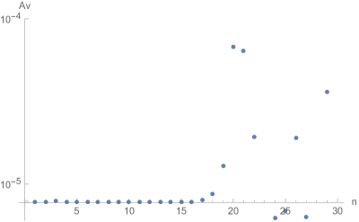
Figure 6: The quantity plotted (for clarity on a logarithmic scale) $\text{Av}=\langle\frac{I_{n}-I_{n,\text{num}}}{I_{n}}\rangle$ is the weighted difference between the numerical integration $I_{\Delta=1,n}$ in equation (A.32) and the corresponding analytical result, averaged over $0<\chi<1$ for a number of external points ranging from $n=3$ to $n=17$. For this range, the leading error comes from the machine precision in the integral near the endpoints and thus is of the same order for $n=3$ and $n=17$. For higher $n$, the numerical stability of the integral becomes problematic and the numerical results should not be trusted.

A second check of validity can be made through analytical comparisons with known results. The results for $n=3$ and $n=4$ are well known but become sparser as $n$ grows larger, however, pinching also provides a way to compare higher$-n$ results to higher$-\Delta$ four-point correlators, this is done in Appendix A.2.

Appendix B Exchange diagrams

This Appendix contains complementary material relating to the derivation and interpretation of the exchange diagrams. First, details on the conformal Casimir and its relation to the equation of motion in AdS are given. Then the derivation of the relation between exchange diagrams and contact diagrams from [33, 26] is reviewed. This is then applied to the toy model of $\phi^{3}$ interaction in AdS₂, which gives insight into Polyakov blocks whose perturbative strong coupling structure is shown explicitly

Quadratic Casimir

The $n$-Casimir of the boundary conformal group is given by

$$C^{(n)}_{i_{1}..i_{n}}=\frac{1}{2}\{\sum_{k=1}^{n}L_{i_{k}}^{(0)},\sum_{k=1}^{n}L_{i_{k}}^{(0)}\}-\frac{1}{2}[\sum_{k=1}^{n}L_{i_{k}}^{-\alpha},\sum_{k=1}^{n}L_{i_{k}}^{\alpha}],$$ (B.1)

where $L^{(0)}$ are elements of the Cartan and the others are the simple roots. Explicitly for a $d=1$ conformal boundary the differential expression of the operators is:

$$D =L_{0}=\Delta+x\partial_{x} P =L_{-1}=-\partial_{x} K =L_{+1}=-2\Delta x-x^{2}\partial_{x}$$ (B.2)

This leads to a linear Casimir

$$C^{(1)}_{a} =\Delta(\Delta-1),$$ (B.3)

which is the mass-squared of the bulk operator, and a quadratic Casimir:

$$C^{(2)}_{x,y} =2(x-y)(-\Delta_{1}\partial_{y}+\Delta_{2}\partial_{x})-(y-x)^{2}\partial_{x}\partial_{y}+(\Delta_{1}+\Delta_{2}-1)(\Delta_{1}+\Delta_{2}).$$ (B.4)

The quadratic Casimir of the AdS₂ isometries is the Laplacian of AdS, this is best seen in flat embedding coordinates where the generators are given by

$$J_{AB}=-i(X_{A}\partial_{B}-X_{B}\partial_{A}),$$ (B.5)

where $X_{A}X^{A}=1$. The Quadratic casimir of the AdS isometries in embedding coordinates is then

$$-\frac{1}{2}\mathcal{L}_{a}\mathcal{L}^{a} =-\frac{1}{2}J_{AB}J^{AB}$$ (B.6)

$$=\frac{1}{2}(X_{A}\partial_{B}-X_{B}\partial_{A})(X^{A}\partial^{B}-X^{B}\partial^{A})$$ (B.7)

$$=X_{A}X^{A}\partial_{B}\partial^{B}+(1-d)X_{B}\partial^{B}$$ (B.8)

$$=\partial_{A}\partial^{A},$$ (B.9)

which is the coordinate-independent Laplacian.

A case of interest in this paper is when we have $\Delta_{1}=\Delta_{2}$. The conformal quadratic Casimir then simplifies further to

$$C^{(2)}_{z}=2\Delta(2\Delta-1)f(z)-z\left((z-1)zf^{\prime\prime}(z)+(2\Delta(z-2)+z)f^{\prime}(z)\right),$$ (B.10)

where we have made a change of variable

$$z=1-\frac{x}{y}.$$ (B.11)

Such changes of variables can be made to reduce this differential equation into a single variable differential equation for each of the $(s,t,u)$ exchange channels.

B.1 Relating the exchange and contact diagrams

We review the analysis from [49, 25], which goes through a detailed computation of the exchange diagram and the $z$ integral. However, they specialise in the case where the resulting exchange correlator can be written in terms of a finite sum of $D$-functions. The toy model considered in this paper does not satisfy the conditions needed for such a simplification, but still is useful to illustrate the Polyakov blocks.

Figure 7: Exchange Witten diagram for 4 external insertions of identical scalars of weight $\Delta_{\phi}$ exchanging a scalar of weight $\Delta_{E}$ in the $t$ channel

The integral we are interested in, corresponding to the Witten diagram (7), is

$$J^{(t)}(x_{1},...,x_{4}) =\int\frac{d^{2}w}{w_{0}^{2}}I(w,x_{2},x_{3})K_{\Delta_{1}}(x_{1},w)K_{\Delta_{4}}(x_{4},w),$$ (B.12)

$$I(w,x_{2},x_{3}) =\int\frac{d^{2}z}{z_{0}^{2}}G_{\Delta_{E}}(w,z)K_{\Delta_{2}}(x_{2},z)K_{\Delta_{3}}(x_{3},z).$$ (B.13)

The integral $I(z_{a},x_{a};x_{2},x_{3})$ is a boundary-boundary-to-bulk three-point function and has conformal symmetry.

Figure 8: The system is invariant under an infinitesimal transformation (B.14).

$I(w,x_{2},x_{3})$ in (B.13) is invariant under global transformations generated by $\mathbf{\mathcal{L}}_{a}+\vec{L}_{2}+\vec{L}_{3}$, where the first term generates the isometries of $AdS_{2}$ and the other two generate the conformal transformation of the boundary. As such, we can write

$$(\mathbf{\mathcal{L}}_{a}+\vec{L}_{2}+\vec{L}_{3})I(z_{a},x_{a};x_{2},x_{3})=0,$$ (B.14)

and can therefore relate the Casimirs of the generators

$$-\frac{1}{2}\mathbf{\mathcal{L}}_{a}^{2}I(z_{a},x_{a};x_{2},x_{3}) =-\frac{1}{2}(\vec{L}_{2}+\vec{L}_{3})^{2}I(z_{a},x_{a};x_{2},x_{3})$$ (B.15)

$$=C^{(23)}_{2}I(z_{a},x_{a};x_{2},x_{3}).$$ (B.16)

In one dimension, the quadratic Casimir of the $AdS_{2}$ isometries is the Laplacian of the bulk B. This Laplacian will allow us to get rid of the bulk-to-bulk propagator through the equation of motion (2.21). Linking the previous elements together, we obtain

$$(C_{(23)}^{(2)}-m^{2}_{E})I(z_{a},x_{a};x_{2},x_{3}) =(\nabla_{a}^{2}-m_{E}^{2})I(z_{a},x_{a};x_{2},x_{3})$$ (B.17)

$$=K_{\Delta_{\phi}}(z_{a},x_{a};x_{2})K_{\Delta_{\phi}}(z_{a},x_{a};x_{3}).$$ (B.18)

The quadratic Casimir acting on the points 3 and 4 commutes with the other coordinates, so we can write a differential equation relating the full exchange diagram to the contact term

$$(C_{(23)}^{(2)}-m^{2}_{E})J(x_{1},x_{2},x_{2},x_{3}) =\int\frac{dz_{a}dx_{a}}{z_{a}^{2}}\Pi_{i=1}^{4}K_{\Delta_{\phi}}(z_{a},x_{a};x_{i})$$ (B.19)

$$=\frac{A}{(x_{13}x_{24})^{2\Delta_{\phi}}}\bar{D}_{\Delta_{\phi}\Delta_{\phi}\Delta_{\phi}\Delta_{\phi}}(\chi).$$ (B.20)

The same analysis holds for any two legs attached to a bulk-to-bulk propagator, though the final differential equation might depend on many variables.

B.2 Perturbative Polyakov blocks

Polyakov blocks and OPE expansion

It will be useful to illustrate how Polyakov blocks and Conformal blocks operate perturbatively. The four-point correlator of a scalar of conformal dimension $\Delta$ is

$$\langle\phi_{\Delta}(x_{1})\phi_{\Delta}(x_{1})\phi_{\Delta}(x_{1})\phi_{\Delta}(x_{1})\rangle=\frac{(C_{\Delta})^{4}}{(x_{13}x_{24})^{2\Delta}}f(\chi)$$ (B.21)

$$f(\chi)=\sum_{h}c^{2}_{\Delta\Delta h}\chi^{-2\Delta}G_{h}(\chi)=\sum_{h}c^{2}_{\Delta\Delta h}\chi^{-2\Delta}P_{h}(\chi).$$ (B.22)

where $G_{h}$ are the conformal blocks and $P_{h}(\chi)$ are the Polyakov blocks. The four-point conformal blocks in $d=1$ are the eigenfunctions of the quadratic Casimir

$$G_{h}(\chi)=\chi^{h}{}_{2}F_{1}(h,h,2h;\chi).$$ (B.23)

The Polyakov blocks are not eigenvalues of the quadratic Casimir and depend non-trivially on the exchanged and external dimension. Though the Polyakov blocks are not known in closed form in position sapce, their double-discontinuity is equal to that of the conformal blocks in the $t$-channel

$$dDisc[\chi^{-2\Delta}P^{(t)}_{h}(\chi)] =dDisc[\chi^{-2\Delta}G^{(t)}_{h}(\chi)]$$

$$=2\sin^{2}\left(\frac{\pi}{2}(h-2\Delta)\right)(1-\chi)^{-2\Delta}G_{h}(1-\chi).$$ (B.24)

The double-discontinuity of the Polyakov block in the $t$-channel is given by the replacement $\chi\rightarrow 1-\chi$ since the Polyakov block is crossing-symmetric.

$$dDisc[\chi^{-2\Delta}P^{(s)}_{h}(\chi)]=2\sin^{2}\left(\frac{\pi}{2}(h-2\Delta)\right)\chi^{-2\Delta}G_{h}(\chi).$$ (B.25)

If we expand the four-point correlator in a small strong coupling parameter $\epsilon$

$$f(\chi)=f^{0}(\chi)+\epsilon f^{1}(\chi)+O(\epsilon^{2}),$$ (B.26)

one can look at the structure and properties of these two expansions. The first order is Generalised Free Field Theory where the spectrum is $\{0,h=2\Delta+2n\}$, and the correlator is obtained with the pairwise Wick contractions between fields

$$f^{0}(\chi)=1+\chi^{2\Delta}+\left(\frac{\chi}{1-\chi}\right)^{2\Delta}.$$ (B.27)

The conformal decomposition

$$f^{0}(\chi) =1+\sum_{n}c_{2\Delta+2n,\Delta,\Delta}^{2}G_{2\Delta+2n}(\chi),$$ (B.28)

gives the OPE coefficients. Whereas the Polyakov blocks vanish at the position of the double trace operators

$$f^{0}(\chi)=P_{\Delta,0}(\chi)+\sum_{n}c_{n}^{(0)}P_{2\Delta+2n}(\chi),$$ (B.29)

giving the identity contribution in all channels.

$$P_{\Delta,0}(\chi)=1+\chi^{2\Delta}+\left(\frac{\chi}{1-\chi}\right)^{2\Delta}.$$ (B.30)

At first order in a perturbative expansion, assuming that there are no new exchanged operators, the spectrum is $h=\{0,2\Delta+2n+\epsilon\gamma^{(1)}_{n}\}$, where the identity operator receives no corrections. The first order OPE expansion is then

$$f^{1}(\chi) =\sum_{n}c^{(1)}_{n}G_{n}(\chi)+c_{n}^{(0)}\left(\frac{g\gamma_{n}}{2}\right)\partial_{n}G_{n}(\chi)$$ (B.31)

$$=\sum_{n}c_{n}^{(0)}\left(\frac{g\gamma_{n}}{2}\right)\partial_{n}P_{n}(\chi).$$ (B.32)

Only one term in the Polyakov block expansion is non vanishing in this case

$$f^{1}(\chi)=c_{0}^{(0)}\left(\frac{g\gamma_{0}}{2}\right)(\partial_{n}P_{n})|_{n=0}(\chi).$$ (B.33)

If there is a new exchanged operator $\Delta_{E}\neq 2\Delta+2n$ at this order ($c_{\Delta_{E}\Delta\Delta}=O(\sqrt{\epsilon})$), the expansion is changed by a factor:

$$f^{1}(\chi)=c_{0}^{(0)}\left(\frac{g\gamma_{0}}{2}\right)(\partial_{n}P_{n})|_{n=0}(\chi)+c_{\Delta_{E}\Delta\Delta}^{2}P_{\Delta_{E}}(\chi)$$ (B.34)

In the strong coupling language, this corresponds to having an Exchange Witten diagram with exchange dimension $\Delta_{E}$. Hence, the Polyakov blocks are given by exchange Witten diagrams, up to the contact diagram contribution from equation (B.33).

Polyakov blocks and exchange Witten diagrams

The computation of the exchange Witten diagram in the main text (5) is the sum of solutions to second-order differential equations. The integration constants are provided by the three-point function and the symmetry of the correlator. The example given in the main text corresponding to the Polyakov block of external dimension $\Delta=1$ and exchanged dimension $\Delta_{E}=1$ can be computed with the toy model of a massless scalar theory in AdS₂ with a $\phi^{3}$ interaction, this corresponds to the action

$$S_{\phi^{3}}=\int\frac{dtdz}{z^{2}}\left(\partial_{\mu}\phi\partial^{\mu}\phi-\frac{\lambda}{3!}\phi^{3}\right).$$ (B.35)

The leading order is given by GFF. The next to leading order ($O(\lambda)$) correlators come from the constant vertex giving the 3 point function

$$<\phi(x_{1})\phi(x_{2})\phi(x_{3})> =\frac{\lambda}{\pi^{3}}\frac{\pi^{2}}{2x_{12}x_{23}x_{13}},$$ (B.36)

and the OPE coefficient

$$c_{111} =\frac{\lambda}{2\pi}.$$ (B.37)

The first sub-leading term ($O(\lambda^{2})$) in the four-point function is generated by the exchange diagram which contributes

$$<\phi(x_{1})\phi(x_{2})\phi(x_{3})\phi(x_{4})> =\sum_{s,t,u}\lambda^{2}J_{\Delta_{E}=1,\Delta=1}(x_{1},...,x_{4})$$ (B.38)

$$=\frac{\lambda^{2}}{\pi^{5}}\frac{\pi}{4}\frac{1}{(x_{13}x_{24})^{2}}P^{(0)}_{(1,1)}(\chi),$$ (B.39)

where $P^{(0)}_{(1,1)}(\chi)$ is written explicitly in Equation (5) and has a small $\chi$ expansion

$$<\phi(x_{1})\phi(x_{2})\phi(x_{3})\phi(x_{4})> =\frac{1}{(x_{13}x_{24})^{2}}\frac{\lambda^{2}}{4\pi^{4}}\left(\frac{c_{1}-6\zeta(3)}{\chi^{2}}+\frac{2\left(\pi^{2}-3c_{2}\right)}{3\chi}\right)+o\left(\frac{1}{\chi}\right).$$ (B.40)

The first term in the expansion is set to zero since it corresponds to a correction to the identity operator. The second term corresponds in the conformal s-channel OPE to

$$\frac{1}{(x_{13}x_{24})^{2}}\sum_{h}c_{11h}^{2}\chi^{h-2}{}_{2}F_{1}(h,h,2h,\chi) =\frac{1}{(x_{13}x_{24})^{2}}\left(\frac{c_{111}^{2}}{\chi}+o\left(\frac{1}{\chi}\right)\right),$$ (B.41)

where by equating the expansions in the conformal and Polyakov blocks, this corresponds to $c_{\Delta_{E}\Delta\Delta}$ in equation (B.34). The known three-point function and the four-point OPE then give the solutions for the integration constants

$$c_{1}=6\zeta(3)$$ (B.42)

$$c_{2}=-\frac{\pi^{2}}{6},$$ (B.43)

and provide the correct numerical factor for the Polyakov block computed in the main text as well as the maximally symmetric and Regge-bounded function.

B.3 Higher weight exchange diagrams and bootstrap

The process done in the main text can be repeated for other exchanged weights, for example we have the s-channel exchanges

$$f^{(s)}_{\Delta_{E}=2}(\chi) =\frac{4c_{2}-4\chi\log^{2}(\chi)+8\chi\log(\chi)+2\log(1-\chi)(2\chi\log(\chi)-4)+\frac{4\pi^{2}}{3}}{\chi^{3}}$$ (B.44)

$$+\frac{2(\chi-2)}{\chi^{3}}\left(c_{1}-c_{2}\log(1-\chi)-\text{Li}_{2}(\chi)\log\left(\frac{1-\chi}{\chi^{2}}\right)-\text{Li}_{3}(1-\chi)-2\text{Li}_{3}(\chi)\right.$$

$$+\left.\log\left(\frac{\chi}{1-\chi}\right)\log(1-\chi)\log(\chi)\right)$$

$$f^{(s)}_{\Delta_{E}=3} =-\frac{2((\chi-6)\chi+6)(+3\text{Li}_{3}(1-\chi)+\log(1-\chi)(\text{Li}_{2}(\chi)+\log(1-\chi)\log(\chi)))}{\chi^{4}}$$ (B.45)

$$-\frac{6(\chi-2)(2\text{Li}_{2}(\chi)+\log(1-\chi)\log(\chi))}{\chi^{3}}$$

$$+\frac{2\left(9\chi^{2}\log(\chi)+\left(\pi^{2}((\chi-6)\chi+6)-9\left(\chi^{2}+\chi-3\right)\right)\log(1-\chi)\right)}{3\chi^{4}}$$

$$+2\frac{\left(\pi^{2}(\chi-3)-9(\chi-4)\right)(\chi-1)}{\chi^{4}}$$

$$f^{(s)}_{\Delta_{E}=4} =-\frac{2(\chi-2)\left(\chi^{2}-10\chi+10\right)}{\chi^{5}}\Big{(}\text{Li}_{2}(\chi)\log\left(\frac{1-\chi}{\chi^{2}}\right)$$ (B.46)

$$\qquad+\text{Li}_{3}(1-\chi)+2\text{Li}_{3}(\chi)+\log(\chi)\log^{2}(1-\chi)-\log^{2}(\chi)\log(1-\chi)\Big{)}$$

$$+\frac{2\left(11\chi^{2}-60\chi+60\right)(\log(1-\chi)-\log(\chi))\log(\chi)}{3\chi^{4}}$$

$$+\frac{8\chi(\chi(19\chi-90)+90)\log(\chi)-2(\chi-1)(\chi(76\chi-335)+310)\log(1-\chi)}{9\chi^{5}}$$

$$+\frac{10(\chi(2(104-9\chi)\chi-505)+330)+2\pi^{2}(\chi((336-25\chi)\chi-885)+610)}{9\chi^{5}}$$

As we increase the weight of the exchanged operator, this seemingly increases the complexity of the solution, however, there are some patterns that are easy to spot. Notice that all transcendentality 3 terms have the same polynomial function multiplying them motivating the use a transcendentality ansatz [10]:

$$\sum_{n,i}r_{i,n}(\chi)T_{i_{n}}(\chi)$$ (B.47)

And inserting it in the differential equations, we obtain differential equations for the polynomials multiplying the transcendentality $i$ functions for arbitrary weight $\Delta_{E}$ and arbitrary external weights $\Delta$. In particular, the polynomials multiplying the transcendentality 3 terms remaining after the action of the Casimir differential operator will satisfy the homogeneous differential equation. Explicitly we have

$$r_{3,n}^{(s)} =c_{n}\chi^{-2\Delta-\Delta_{E}+1}\,_{2}F_{1}(1-\Delta_{E},1-\Delta_{E};2-2\Delta_{E};\chi)$$ (B.48)

$$r_{3,n}^{(t)} =c_{n}(1-\chi)^{-2\Delta-\Delta_{E}+1}\,_{2}F_{1}(1-\Delta_{E},1-\Delta_{E};2-2\Delta_{E};1-\chi)$$ (B.49)

$$r_{3,n}^{(u)} =P_{\Delta_{E}-1}(2\chi-1)$$ (B.50)

The transcendentality 2 functions are multiplied by polynomials that satisfy inhomogeneous differential equations and are difficult to solve for general $\Delta_{E}$. However, for specific cases, they are simple to solve. We can do this for example for higher exchanged weights and more importantly, for higher-point correlators with exchanges. This analysis is beyond the scope of this paper and left for further investigation

Appendix C Multipoint Ward identity: a check

A concrete example of $n$-point correlators of fields at the boundary of AdS₂ is the dual setup of the defect CFT of operator insertions on the 1/2 BPS Wilson line in $\mathcal{N}=4$ SYM studied at strong coupling in [1, 2]. In higher-point correlators, the first terms in the strong coupling expansion will originate from disconnected Witten diagrams. These first terms in the strong coupling expansion should satisfy the multipoint Ward identity presented in [36], therefore providing a perturbative check of these conjectured Ward identities

$$\sum_{k=1}^{n-3}\left(\frac{1}{2}\partial_{\chi_{k}}+\alpha_{k}\partial_{r_{k}}-(1-\alpha_{k})\partial_{s_{k}}\right)\mathcal{A}_{\Delta_{1}...\Delta_{n}}\raisebox{-5.69046pt}{$\Biggr{|}$}_{\raisebox{5.69046pt}{$\begin{subarray}{l}r_{i}\rightarrow\alpha_{i}\chi_{i}\\ s_{i}\rightarrow(1-\alpha_{i})(1-\chi_{i})\\ t_{ij}\rightarrow(\alpha_{i}-\alpha_{j})(\chi_{i}-\chi_{j})\end{subarray}$}}=0$$ (C.1)

where we use the notation of [36] in which the cross-ratios are defined as

$$\chi_{i-1} =\frac{x_{1i}x_{n-1,n}}{x_{in}x_{1,n-1}}$$ (C.2)

$$r_{i-1} =\frac{(u_{1}\cdot u_{i})(u_{n-1}\cdot u_{n})}{(u_{i}\cdot u_{n})(u_{1}\cdot u_{n-1})}$$ (C.3)

$$s_{i-1} =\frac{(u_{1}\cdot u_{n})(u_{i}\cdot u_{n-1})}{(u_{i}\cdot u_{n})(u_{1}\cdot u_{n-1})}$$ (C.4)

$$t_{i-1,j-1} =\frac{(u_{i}\cdot u_{j})(u_{1}\cdot u_{n})(u_{n-1}\cdot u_{n})}{(u_{i}\cdot u_{n})(u_{j}\cdot u_{n})(u_{1}\cdot u_{n-1})},$$ (C.5)

and the Ward identity is applied to the correlator of dimension $\Delta=1$, SO(5) vectors expressed in terms of cross-ratios

$$\langle\Pi_{i=1}^{6}u_{a_{i}}\Phi^{a_{i}}(x_{i})\rangle=C(x_{i},u_{i})\mathcal{A}_{\Delta=1,n=6}(\chi_{i},r_{i},s_{i},t_{i,j})$$ (C.6)

where the prefactor

$$C(x_{i},u_{i})=\frac{(u_{1}.u_{5})^{2}(u_{2}.u_{6})(u_{3}.u_{6})(u_{4}.u_{6})}{(u_{1}.u_{6})(u_{5}.u_{6})}\frac{x_{16}^{2}x_{56}^{2}}{x_{15}^{4}x_{26}^{2}x_{36}^{2}x_{46}^{2}},$$ (C.7)

has been amputated. The strong coupling expansion of this quantity is given by the holographic dual studied in [1], where the dual of these particular fields are the fluctuations in the S⁵ directions propagating in the AdS₂ minimal string surface. If we denote the strong coupling expansion parameter by $g$, we can expand the six-point function at strong coupling

$$\mathcal{A}_{\Delta=1,n=6}(\chi_{i},r_{i},s_{i},t_{i,j}) =\mathcal{A}^{(0)}_{\Delta=1,n=6}(\chi_{i},r_{i},s_{i},t_{i,j})+g\mathcal{A}^{(1)}_{\Delta=1,n=6}(\chi_{i},r_{i},s_{i},t_{i,j})+O(g^{2})$$ (C.8)

Given the Ward identity is coupling independent, each of the terms in this perturbative expansion should satisfy equation (C.1) . The leading term, $\mathcal{A}^{(0)}_{\Delta=1,n=6}$, in the strong coupling expansion corresponds to the simple Wick contractions where a few examples are drawn in 9.

Figure 9: A non-exhaustive list of leading order disconnected Witten diagram. The overlapping lines are broken to indicate they are not vertices, it is not a non-planar contribution at strong coupling, since we are in the strict planar limit.

Explicitly, performing these permutations, we find

$$\mathcal{A}^{(0)}_{\Delta=1,n=6} =\frac{r_{3}t_{1,2}}{\left(\chi_{1}-\chi_{2}\right){}^{2}\chi_{3}^{2}}+\frac{r_{2}t_{1,3}}{\chi_{2}^{2}\left(\chi_{1}-\chi_{3}\right){}^{2}}+\frac{r_{1}t_{2,3}}{\chi_{1}^{2}\left(\chi_{2}-\chi_{3}\right){}^{2}}+\frac{s_{1}t_{2,3}}{\left(\chi_{1}-1\right){}^{2}\left(\chi_{2}-\chi_{3}\right){}^{2}}$$

$$+\frac{s_{3}t_{1,2}}{\left(\chi_{1}-\chi_{2}\right){}^{2}\left(\chi_{3}-1\right){}^{2}}+\frac{s_{2}t_{1,3}}{\left(\chi_{2}-1\right){}^{2}\left(\chi_{1}-\chi_{3}\right){}^{2}}+\frac{t_{1,2}}{\left(\chi_{1}-\chi_{2}\right){}^{2}}+\frac{t_{1,3}}{\left(\chi_{1}-\chi_{3}\right){}^{2}}$$

$$+\frac{t_{2,3}}{\left(\chi_{2}-\chi_{3}\right){}^{2}}+\frac{r_{2}s_{1}}{\left(\chi_{1}-1\right){}^{2}\chi_{2}^{2}}+\frac{r_{3}s_{1}}{\left(\chi_{1}-1\right){}^{2}\chi_{3}^{2}}+\frac{r_{1}s_{2}}{\chi_{1}^{2}\left(\chi_{2}-1\right){}^{2}}+\frac{r_{1}s_{3}}{\chi_{1}^{2}\left(\chi_{3}-1\right){}^{2}}$$

$$+\frac{r_{2}s_{3}}{\chi_{2}^{2}\left(\chi_{3}-1\right){}^{2}}+\frac{r_{3}s_{2}}{\left(\chi_{2}-1\right){}^{2}\chi_{3}^{2}}$$ (C.9)

For which, not only is the Ward identity satisfied, but each of the terms in equation (C) corresponding to the different R-symmetry channels individually satisfy this equation. As such, this is a trivial check of this Ward identity. The next-to-leading term corresponds to the disconnected diagram with one Wick contraction and a contact four-point function,

$$\mathcal{A}^{(1)}_{\Delta=1,n=6}(\chi_{i},r_{i},s_{i},t_{i,j})=\frac{r_{1}t_{2,3}G^{(1)}_{4}\left(\frac{\chi_{1}\left(\chi_{2}-\chi_{3}\right)}{\chi_{2}\left(\chi_{1}-\chi_{3}\right)}\right)}{\chi_{1}^{2}\left(\chi_{2}-\chi_{3}\right){}^{2}}+\textrm{permutations }[(x_{i},u_{i})].$$ (C.10)

This corresponds to the permutations of which a few examples are given by the disconnected Witten diagrams in Figure 10.

Figure 10: Some of the next-to-leading order disconnected Witten diagrams

The four-point function is computed in [1] and can be written as

$$\langle\Phi^{a_{1}}(x_{1})\Phi^{a_{2}}(x_{2})\Phi^{a_{3}}(x_{3})\Phi^{a_{4}}(x_{4})\rangle=\frac{\delta^{a_{1}}_{a_{2}}\delta^{a_{3}}_{a_{4}}}{(x_{12}x_{34})^{2}}G_{4}^{(1)}(\frac{x_{12}x_{34}}{x_{13}x_{24}})+\textrm{permutations }[(x_{i},u_{i})]$$ (C.11)

$$G_{4}^{(1)}(\chi)=\frac{(\chi-1)\left(\chi^{2}+\chi+2\right)\log\left((\chi-1)^{2}\right)}{2\chi}\!-\!\frac{\left(\chi^{2}-2\chi+2\right)\left(\chi^{2}\log\left(\chi^{2}\right)-2\chi+2\right)}{2(\chi-1)^{2}}.$$ (C.12)

Just as in the GFF case, each of the R-symmetry channels also satisfy the Ward identities (C.1) individually. As a consequence, this is not constraining for the 6-point function, but rather motivates the consistency of these Ward identities. This seems to follow from the fact that the disconnected contribution can be written as a product of correlators, each satisfying a Ward identity, though this is dependent on the crossing and analytic properties of the four-point function. While it does not give insight into the connected contribution, this seems to indicate a recursive method to prove this Ward identity for any disconnected correlators.