The Potential Method For Price-Formation Models

Abstract

We consider the mean-field game price formation model introduced by Gomes and Saúde. In this MFG model, agents trade a commodity whose supply can be deterministic or stochastic. Agents maximize profit, taking into account current and future prices. The balance between supply and demand determines the price. We introduce a potential function that converts the MFG into a convex variational problem. This variational formulation is particularly suitable for machine learning approaches. Here, we use a recurrent neural network to solve this problem. In the last section of the paper, we compare our results with known analytical solutions.

I Introduction

Mean-field games (MFG) were introduced in [23], [22] as models for systems with a large number of competitive rational agents. In these games, agents take decisions according to preferences given by a utility function. Individually, agents have a negligible effect on the entire system but are affected by aggregate effects. These games arise to model power networks, free markets, social media, or pedestrians flows.

Here, we study the electricity market price formation model from [21]. Note, however, that the same model describes price formation for any commodity that can be traded, stored, and whose price is determined by market clearing conditions. In this model, agents have storage devices and may charge them (buy) or supply (sell) the grid with electricity. Agents maximize profit by trading electricity at a price $\varpi(t)$. The balance between supply, $Q(t)$, and aggregate demand determines the price, $\varpi(t)$. We consider both deterministic and stochastic supply.

I-A Deterministic supply

The deterministic supply, discussed in Section III-A, is outlined in the next problem.

Problem 1

Let $\Theta=[0,T]\times{\mathbb{R}}$. Suppose that $m_{0}\in\mathcal{P}({\mathbb{R}})$, $H\in C^{2}({\mathbb{R}}^{2})$ is uniformly convex, and $Q$ and $u_{T}$ are Lipschitz continuous. Find $u,m:\Theta\to{\mathbb{R}}$ and $\varpi:[0,T]\to{\mathbb{R}}$ satisfying

$$\begin{cases}-u_{t}+H(x,\varpi+u_{x})=0\\ m_{t}-\left(H_{p}(x,\varpi+u_{x})m\right)_{x}=0\\ -\int_{{\mathbb{R}}}H_{p}(x,\varpi+u_{x})m{\rm d}x=Q(t),\end{cases}$$ (1)

$m\geqslant 0$, and the initial-terminal conditions

$$m(0,x)=m_{0}(x),\quad u(T,x)=u_{T}(x).$$ (2)

Existence and uniqueness of solutions was addressed in [21]. [9] examined the connection between Aubry-Mather theory and Problem 1.

In [10], following the ideas in [11], we introduce a potential function $\varphi:\Theta\to{\mathbb{R}}$ giving for each $t$ the cumulative distribution of $m$. Further, $\varphi_{x}=m$ and $-\varphi_{t}$ is the agents’ current or flow. There, we formulate a variational problem and show that (1) is the corresponding Euler-Lagrange equation, see Section III-A. To detail this problem, we let $L$ be the Legendre transform of $H$, $L(x,v)=\sup_{p\in{\mathbb{R}}}\left[-pv-H(x,p)\right]$. We assume that $L$ and $H$ are uniformly convex in the second variable and that, for some $c,p>0$, $L(x,v)\geqslant c|v|^{p}$. Further, let $F:{\mathbb{R}}^{2}\times{\mathbb{R}}_{0}^{+}\to{\mathbb{R}}_{0}^{+}$ be the perspective function of $L$

$$F(x,j,m)=\begin{cases}L\left(x,\frac{j}{m}\right)m,&m>0\\ +\infty,&j\neq 0,\,m=0\\ 0,&j=0,\,m=0.\end{cases}$$

The constrained variational problem corresponding to Problem 1 is as follows.

Problem 2

Consider the setting of Problem 1. Find $\varphi:\Theta\to{\mathbb{R}}$ minimizing

$$\int_{\Theta}F(x,-\varphi_{t},\varphi_{x})-u^{\prime}_{T}(x)\varphi_{t}~{}{\rm d}x{\rm d}t,$$

over all functions s.t. $\varphi(0,x)=\int_{-\infty}^{x}m_{0}(y){\rm d}y$, and, for all $t\in[0,T]$, $\varphi_{x}(t,\cdot)\in\mathcal{P}({\mathbb{R}})$ and

$$\int_{{\mathbb{R}}}\varphi(t,x)-\varphi(0,x){\rm d}x=-\int_{0}^{t}Q(s){\rm d}s.$$

The functional to be minimized in the prior problem represents an average social cost; the constraint reflects the balance condition. In [10], we analyzed Problem 2. There, we obtained the correspondence between Problems 1 and 2 and proved the existence of the price, $\varpi$, as a Lagrange multiplier.

I-B Stochastic supply

The stochastic supply case was studied in [20] for the continuum, and in [19] for $N$ players; the authors obtained a price as a Lagrange multiplier for the balance constraint. In the stochastic case, discussed in Section II-B, the corresponding problem is as follows.

Problem 3

Consider the setting of Problem 1. Let $(\Omega,{\mathcal{F}},P)$ be a probability space that supports a standard Brownian motion $W_{t}$. Let ${\mathcal{F}}_{t}$ be the filtration generated by $W_{t}$ and let $Q$ be a progressively measurable process (PMP) with respect to ${\mathcal{F}}_{t}$. Find $m:\Theta\to{\mathbb{R}}$ and $u$, $Z$ and $\varpi$, PMP with respect to ${\mathcal{F}}_{t}$, satisfying $m\geqslant 0$, (2), and

$$\begin{cases}-du+H(x,\varpi+u_{x})dt=Z(x,t)dW_{t}\\ m_{t}-\left(H_{p}(x,\varpi+u_{x})m\right)_{x}=0\\ -\int_{{\mathbb{R}}}H_{p}(x,\varpi+u_{x})m{\rm d}x=Q(t).\end{cases}$$ (3)

Next, in Section III-C, we introduce a progressively measurable potential, $\varphi$ and derive the following stochastic variational problem associated with Problem 3.

Problem 4

Consider the setting of Problem 3. Find a progressively measurable function $\varphi:\Theta\times\Omega\to{\mathbb{R}}$ minimizing

$$E\int_{\Theta}F(x,-\varphi_{t},\varphi_{x})-\varpi\left(\varphi_{t}+Q\varphi_{x}\right)-u^{\prime}_{T}\varphi_{t}~{}{\rm d}x{\rm d}t$$

over the set of PMP $\varphi$ such that $\varphi(0,x)=\int_{-\infty}^{x}m_{0}(y){\rm d}y$, and for all $t\in[0,T]$ satisfy $\varphi_{x}(t,\cdot)\in\mathcal{P}({\mathbb{R}})$ and

$$\int_{{\mathbb{R}}}\varphi(t,x)-\varphi(0,x){\rm d}x=-\int_{0}^{t}Q(s){\rm d}s.$$

In section IV, we parametrize the potential by a recurrent neural network (RNN) and use the variational problem as the residual. RNN preserve progressive measurability and give a compact way to represent the potential. This is particularly relevant in the random case where the problem is infinite-dimensional. In Section V, we illustrate our approach for the linear-quadratic setting and take as benchmarks the explicit formulas provided in [21] and [20].

I-C Prior work

In [6] and [7], MFG models were used to describe intraday electricity markets. There, the price is a function of the demand rather than being determined by market clearance. In [15], the authors considered a Stackelberg game of an intraday market, where a major agent faces many small agents. A similar problem with a major player was studied in [18]. Using stochastic control theory, in [16], the authors studied renewable energy markets in the $N$-agent and MFG settings. A deterministic $N$-agent price model was considered in [8] and in [19]. Also, a $N$-agent price model was examined in [4]. There, the price is determined by the equilibrium of the system; the agents choose optimal controls (production and trading rates) to meet a demand with noise. In [12], [24], Stackelberg games modeled price formation under revenue optimization. To study price dynamics in electricity market in [14], the authors considered Cournot model and showed that their model is a MFG problem with common noise and a jump-diffusion. The paper [5] modeled the transition to renewable energies by an optimal switching MFG. The works [25] and [17] used market-clearing conditions to study Solar Energy Certificate Markets and flows in exchange markets, respectively.

Because there are only a few MFG models with explicit solutions, numerical analysis of MFGs plays a crucial role, see the survey [3] and the earlier works in [1] and [2]. However, prior methods cannot be used directly for our model because the price, $\varpi$, must satisfy an integral constraint. In [10], we introduced a numerical scheme for Problem 1, which solves a convex minimization problem. In the case of common noise, this matter is more delicate because the state space becomes infinite-dimensional. A state-space reduction strategy was developed in [20] and the $N$ player case was studied in [19], but none of the prior references addressed this problem in full generality.

I-D Main contributions

This paper contains the following contributions. We present a novel formulation of the price problem with a random supply as a stochastic MFG system (Problem 3), extending prior works limited to the linear-quadratic and $N$-player cases. We developed a potential approach for the random supply problem by introducing a stochastic variational problem (Problem 4). Finally, we used RNN to solve both the deterministic and stochastic price problems (Problems 2 and 4). Because the stochastic case is infinite-dimensional, the use of RNN seems to beat the curse of dimensionality.

II Control problem associated with the price model

Now, we describe the price formation model.

II-A Deterministic price problem derivation

Consider a deterministic supply $Q$. Given the price $\varpi$, each agent chooses a control $v:[t,T]\to{\mathbb{R}}$ that minimizes

$$u(x,t)=\inf_{v}\int_{t}^{T}L({\bf x},v)+\varpi v+u_{T}({\bf x}(T)).$$

By the HJ verification theorem, if $u$ solves the first equation in (1), $u$ is the value function and $v^{*}=-H_{p}(x,\varpi+u_{x})$ an optimal control. Because agents are rational, they use this optimal strategy; hence, $\dot{\bf x}=v^{*}(t)$. Thus, the density $m$ solves the transport equation, the second equation in (1). While we assumed the price to be known, this MFG is a fixed point: the price must be consistent with the last identity in (1) that requires aggregated total demand (left-hand side) to match supply (right-hand side).

II-B Stochastic price problem derivation

Consider the setting of Problem 3. Assume that $Q$ and $\varpi$ are PMP with respect to ${\mathcal{F}}_{t}$. Let $E_{t}[Z]=E[Z|{\mathcal{F}}_{t}]$, for any random variable $Z$. Each agent chooses a PMP ${\bf v}$ to minimize

$$u(x,t)=E_{t}\int_{t}^{T}L({\bf x},{\bf v})+\varpi{\bf v}+u_{T}({\bf x}(T)),$$ (4)

where $\dot{\bf x}={\bf v}$ and ${\bf x}(t)=x$.

Theorem 1

Let $u$ and $Z$ be PMP solving the stochastic HJ equation, the first equation in (3). Then, $u$ is the value function and $v=-H_{p}(x,\varpi+u_{x})$ is an optimal control.

Remark 1

Note that the unknowns in the HJ equation are both $u$ and $Z$; the additional unknown $Z$ ensures progressive measurability.

Proof:

We have

$$E_{t}\int_{t}^{T}L({\bf x},{\bf v})+\varpi{\bf v}ds+u_{T}({\bf x}(T))$$

$$=u(x,t)+E_{t}\int_{t}^{T}L({\bf x},{\bf v})+\varpi vds+du$$

$$\geqslant u(x,t),$$

by the first equation in (3) and the definition of $L$. Because equality holds when $v=-H_{p}(x,\varpi+u_{x})$, the claim follows. ∎

Because agents are rational, each agent evolves according to $\dot{\bf x}=-H_{p}({\bf x},\varpi+u_{x})$. This is an ODE with a random vector field. Accordingy, $m$ solves the (random) transport equation, the second equation in (3). Finally, we require the balance condition in (3) to hold.

III Potential Approach

Here, we describe the potential approach for our models. This approach was introduced in [11], where one-dimensional first- and second-order MFG planning problems were examined.

III-A Deterministic price

We begin our analysis by addressing the transport equation in (1). Let $(u,m,\varpi)$ solve (1) with $m>0$. The transport equation can be written as $\text{div}_{(t,x)}\left(m,-H_{p}(x,\varpi+u_{x})m\right)=0.$ Hence, by Poincaré lemma (see [13], Theorem 1.22), there exists $\varphi:\Theta\to{\mathbb{R}}$ such that

$$m=\varphi_{x},\quad H_{p}(x,\varpi+u_{x})m=\varphi_{t}.$$ (5)

Differentiating the Hamilton-Jacobi equation in (1) with respect to $x$ and using (5), we rewrite the problem (1)-(2) in terms of $\varphi$

$$\begin{cases}\left(H\left(x,-D_{v}L\left(x,-\tfrac{\varphi_{t}}{\varphi_{x}}\right)\right)\right)_{x}\\ \qquad+\left(D_{v}L\left(x,-\tfrac{\varphi_{t}}{\varphi_{x}}\right)+\varpi\right)_{t}=0,\\ -\int_{{\mathbb{R}}}\varphi_{t}+Q\varphi_{x}~{}{\rm d}x=0,\end{cases}$$ (6)

with $\varphi_{x}(0,\cdot)=m_{0}(\cdot)$ and

$$-D_{v}L\left(x,-\frac{\varphi_{t}(T,x)}{\varphi_{x}(T,x)}\right)-\varpi(T)=u^{\prime}_{T}(x).$$ (7)

Simple computations show that (6) and (7) are the Euler-Lagrange equations for the functional

$$\begin{split}\int_{\Theta}F(x,-\varphi_{t},\varphi_{x})-\varpi\left(\varphi_{t}+Q\varphi_{x}\right)-u^{\prime}_{T}\varphi_{t}~{}{\rm d}x{\rm d}t.\end{split}$$

$\varpi$ can be seen as a Lagrange multiplier for the constraint $\int_{{\mathbb{R}}}\varphi_{t}+Q\varphi_{x}~{}{\rm d}x=0$. Thus, we obtain Problem 2. Further, let $\varphi\in C^{2}(\Theta)$ solves Problem 2. Then, we recover the solution $(u,m,\varpi)$ to Problem 1 as follows. We set $m=\varphi_{x},$ and $u(t,x)$ is given by

$$u_{T}(x)-\int_{t}^{T}H\left(x,-D_{v}L\left(x,\tfrac{-\varphi_{t}(s,x)}{\varphi_{x}(s,x)}\right)\right){\rm d}s.$$

$\varpi$ is given by the first equation of (6) and (7).

III-B Fundamental lemmas of the calculus of variations in random environments

Before we discuss the random supply case, we need some preliminary definitions. We consider the following spaces of functions $L^{2}=L^{2}(\Theta\times\Omega)$, which consists of all PMP which are square-integrable in $\Theta\times\Omega$ and $H^{1}=H^{1}(\Theta\times\Omega)$, which contains all PMP, $\phi\in L^{2}$, such that $\phi_{t},\phi_{x}\in L^{2}$. Note for a processe $\psi\in H^{1}$, $d\psi=\psi_{t}dt$; that is, its quadratic variation vanishes. We also consider the space $\tilde{H}(\Theta\times\Omega)$ of processes $\psi\in L^{2}$ such that its stochastic differential $d\psi=adt+bdW_{t}$ exists with $a,b\in L^{2}$. Let $\psi\in\tilde{H}$ and $\phi\in H^{1}$. Then, we have the following identity

$$E\int_{\Theta}\psi\phi_{t}=-E\int_{\Theta}d(\psi)\phi$$ (8)

if $\phi(x,T)=\phi(x,0)=0$. Moreover, if $a,b\in L^{2}$ and we have

$$E\int_{\Theta}\varphi(adt+bdW_{t})=0,$$ (9)

for all $\varphi\in L^{2}$ then $a=0$.

III-C Common noise case

Sufficiently regular critical points of functional in Problem 4 satisfy the weak form of the Euler-Lagrange equation

$$E\int_{\Theta}-F_{j}\phi_{t}+F_{m}\phi_{x}-\varpi\phi_{t}dxdt=0,$$

for all $\phi\in H^{1}$. Assume that $F_{j},\varpi\in\tilde{H}$. By combining the integration by parts formula and the fundamental lemma, we get

$$-d(-F_{j}-\varpi)-(F_{m})_{x}dt=RdW_{t}.$$ (10)

Next, we define $m$ and $u$ according to (5), and set $R=Z_{x}$. Because of (5), we have

$$\varpi+u_{x}=-D_{v}L\big{(}x,-\tfrac{\varphi_{t}}{\varphi_{x}}\big{)}=-F_{j}\big{(}x,-\varphi_{t},\varphi_{x}\big{)}.$$

Further, the definition of $F$, yields

$$F_{m}(x,-\varphi_{t},\varphi_{x})$$

$$=L\big{(}x,-\tfrac{\varphi_{t}}{\varphi_{x}}\big{)}+D_{v}L\big{(}x,-\tfrac{\varphi_{t}}{\varphi_{x}}\big{)}\tfrac{\varphi_{t}}{\varphi_{x}}$$

$$=-H(x,\varpi+u_{x}).$$

Therefore (10) can be rewritten as

$$\begin{split}-d(u_{x})+(H(x,\varpi+u_{x}))_{x}dt=RdW_{t},\end{split}$$

which is the (weak) derivative of the stochastic HJ equation in (3).

IV Machine learning architecture

To approximate $\varphi$, we consider a RNN. A hidden state, $\mathrm{h}$, carries information about the path history. Thus, the outputs of this architecture depend on the path history and guarantee their progressive measurability. Our RNN has a hidden layer followed by three dense layers. The cell of the RNN that we iterate over time is depicted in Fig. 1; the blue arrows highlight the connection along the temporal component.

Figure 1: RNN cell computation at time level $k$. $\mathrm{S}$ denotes the sigmoid function.

The NN architecture depends on a hyper-parameter $\tau$ than includes all weights $\mathrm{W}$ and biases $\mathrm{b}$ defining the NN. The hyper-parameter $\tau$ is optimized to decrease $\mathcal{L}$ by a gradient-descent method at each training step. Let $\varphi_{\Theta}^{\langle k\rangle(i)}$ denote the NN approximation of $\varphi(t_{k},x_{i})$, where $t_{k}$ and $x_{i}$ belong to the time and space grids, respectively. The loss function encodes all the required constraints on the potential. Let

$$\mathcal{L}_{\mathcal{V}}(\varphi_{\tau})=$$

$$h_{x}h_{t}\sum_{k=1}^{M_{t}}\sum_{i=1}^{M_{x}}\left\{F\left(x^{(i)},-\partial_{t}\varphi_{\tau}^{\langle k\rangle(i)},\partial_{x}\varphi_{\tau}^{\langle k\rangle(i)}\right)\right.$$

$$\quad\left.-u^{\prime}_{T}(x^{(i)})\partial_{t}\varphi_{\tau}^{\langle k\rangle(i)}\right\},$$

$$\mathcal{L}_{0}(\varphi_{\tau})=\sum_{k=1}^{M_{t}}\sum_{i=1}^{M_{x}}\max\left\{-\partial_{x}\varphi_{\tau}^{\langle k\rangle(i)},0\right\},$$

$$\mathcal{L}_{\mathcal{B}}(\varphi_{\tau})=\sum_{k=1}^{M_{t}}\left(h_{x}\sum_{i=1}^{M_{x}}\partial_{t}\varphi_{\tau}^{\langle k\rangle(i)}+Q^{\langle k\rangle}\right)^{2},$$

$$\mathcal{L}_{M_{0}}(\varphi_{\tau})=\sum_{i=1}^{M_{x}}\left(\varphi_{\tau}^{\langle 0\rangle(i)}-M_{0}(x^{(i)})\right)^{2},$$

$$\mathcal{L}_{\mathcal{P}}(\varphi_{\tau})=\sum_{k=1}^{M_{t}}\left(1-h_{x}\sum_{i=1}^{M_{x}}\partial_{x}\varphi_{\tau}^{\langle k\rangle(i)}\right)^{2}.$$

$\mathcal{L}_{\mathcal{V}}$ corresponds to the discretization of the variational functional. Deviations from the balance constraint are penalized by $\mathcal{L}_{\mathcal{B}}$, and the initial condition is enforced in $\mathcal{L}_{M_{0}}$. Moreover, $\mathcal{L}_{0}$ and $\mathcal{L}_{\mathcal{P}}$ guarantee that $\varphi_{x}(t,\cdot)$ is a density function. Therefore, we consider the loss function

$$\mathcal{L}=\mathcal{L}_{\mathcal{V}}+\mathcal{L}_{0}+\mathcal{L}_{\mathcal{B}}+\mathcal{L}_{M_{0}}+\mathcal{L}_{\mathcal{P}}$$

that enforces the constraints by penalization.

IV-A Deterministic price

At each training step, we evaluate the supply at points on the time grid. Then, for each time level $k$, we compute $\mathrm{h}^{\langle k\rangle}$, which depends on $(t^{\langle i\rangle},Q^{\langle i\rangle})$ for $i\leqslant k$. Next, we use $\mathrm{h}^{\langle k\rangle}$ for all points $x^{(i)}$ in the state grid. Fig. 1 illustrates the computation at time level $k$. After iterating over time steps, we obtain the NN approximation of the potential, $\varphi_{\tau}$, at grid points, and we compute $\mathcal{L}$. This process is summarized in Table I.

TABLE I: Deterministic training step $j$.

	Input: $M_{0}$, $Q$, $\tau^{j-1}$.
1	for $k=1,\ldots,M_{t}$ do
2	$\quad\mbox{compute }\mathrm{h}^{\langle k\rangle}$
3	$\quad\mbox{for }i=1,\ldots,M_{x}$ do
4	$\quad\quad\mbox{compute }\varphi_{\tau^{j-1}}(t^{\langle k\rangle},x^{(i)})$
5	compute $\mathcal{L}(\varphi_{\tau^{j-1}})$
6	compute $\tau^{j}$ by gradient descend
	Output: $\tau^{j}$

IV-B Random price

The training step follows the same structure as the deterministic case, except for the supply input that is used; we compute a new random supply sample for each training step. The training algorithm is outlined in Table II.

TABLE II: Stochastic training step $j$.

	Input: $M_{0}$, $dQ$, $\tau^{j-1}$.
1	Compute sample $Q_{j}$
2	for $k=1,\ldots,M_{t}$ do
3	$\quad\mbox{compute }\mathrm{h}^{\langle k\rangle}$
4	$\quad\mbox{for }i=1,\ldots,M_{x}$ do
5	$\quad\quad\mbox{compute }\varphi_{\tau^{j-1}}(t^{\langle k\rangle},x^{(i)})$
6	compute $\mathcal{L}(\varphi_{\tau^{j-1}})$
7	compute $\tau^{j}$ by gradient descend
	Output: $\tau^{j}$

V Numerical results

Here, we take $L(x,v)=\tfrac{1}{2}v^{2}$ without terminal cost. We select $T=1$ and $M_{t}=17$ equally spaced grid points for the time variable. We discretize the space variable interval $[-1,1]$ with $M_{x}=31$ equally spaced points. We set $Q(0)=-0.5$, and $m_{0}$ is a symmetric and compactly supported distribution within $[-1,1]$. We discretize the partial derivatives as

$$\partial_{t}\varphi_{\tau}^{\langle k\rangle(i)}=\tfrac{1}{h_{t}}\left(\varphi_{\tau}^{\langle k+1\rangle(i)}-\varphi_{\tau}^{\langle k\rangle(i)}\right),$$

$$\partial_{x}\varphi_{\tau}^{\langle k\rangle(i)}=\tfrac{1}{h_{x}}\left(\varphi_{\tau}^{\langle k\rangle(i+1)}-\varphi_{\tau}^{\langle k\rangle(i)}\right).$$

To guarantee we obtain an approximation of the potential and price on the boundary of $[0,1]\times[-1,1]$, we extend the grid to $[0,1+h_{t}]\times[-1,1+h_{x}]$. The ML method is implemented in TensorFlow with Adam optimizer. The dimension of the hidden state is $32$.

V-A Deterministic case

We assume the supply follows the ODE

$$dQ(t)=\theta\left(\overline{Q}-Q(t)\right)dt,$$

on $[0,T]$, where $\theta=2$ and $\overline{Q}=1$. In this case, $\varpi=-Q$ [21]. Fig. 2 shows the price obtained after $18.000$ training steps. The approximation for $m=\varphi_{x}$ is shown in Figure 3. For the analytical solution, we have $\mathcal{L}=\mathcal{L}_{\mathcal{V}}=0.127604$, since $\mathcal{L}_{0}$, $\mathcal{L}_{\mathcal{B}}$, $\mathcal{L}_{M_{0}}$, and $\mathcal{L}_{\mathcal{P}}$ evaluate to zero. For the NN approximation, we get $\mathcal{L}_{\mathcal{V}}(\varphi_{\tau})=0.134984$. These results illustrate an excellent fit for the price function and a good representation of $m$, including its positivity.

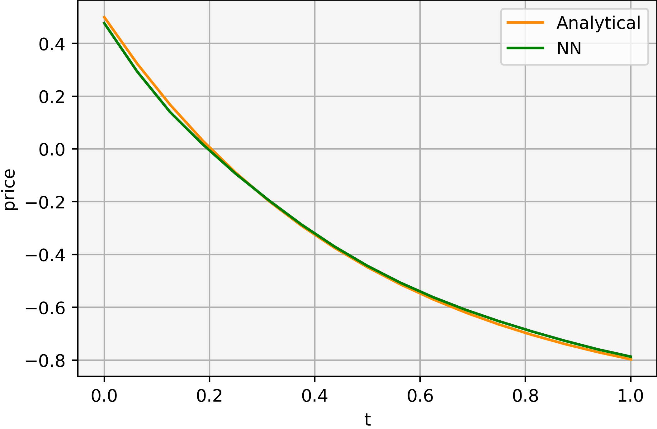
Figure 2: Deterministic price approximation

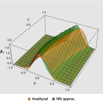
Figure 3: $m=\varphi_{x}$ approx. (left) and error (right).

V-B Stochastic case

We consider a mean-reverting supply

$$dQ(t)=\theta\left(\overline{Q}-Q(t)\right)dt+\sigma dW(t),$$

on $[0,T]$, where $\sigma=0.2$. According to [20], the SDE for the price is $d\varpi=-dQ$. To obtain convergence of our algorithm, we increase the training steps to $36000$. We assess the price approximation using a test set of $1000$ samples of the supply, obtaining an $L^{\infty}$ mean error of $0.036619$. For three samples of the supply, Fig. 4 shows the approximated price, and Figure 5 shows the approximated $m$. We get

$$\mathcal{L}_{\mathcal{V}}(\varphi_{\tau})=0.141007,\;\mathcal{L}_{0}(\varphi_{\tau})=0,$$

$$\mathcal{L}_{\mathcal{B}}(\varphi_{\tau})=0.002728,\;\mathcal{L}_{M_{0}}(\varphi_{\tau})=0.007506,$$

$$\mathcal{L}_{\mathcal{P}}(\varphi_{\tau})=0.01905.$$

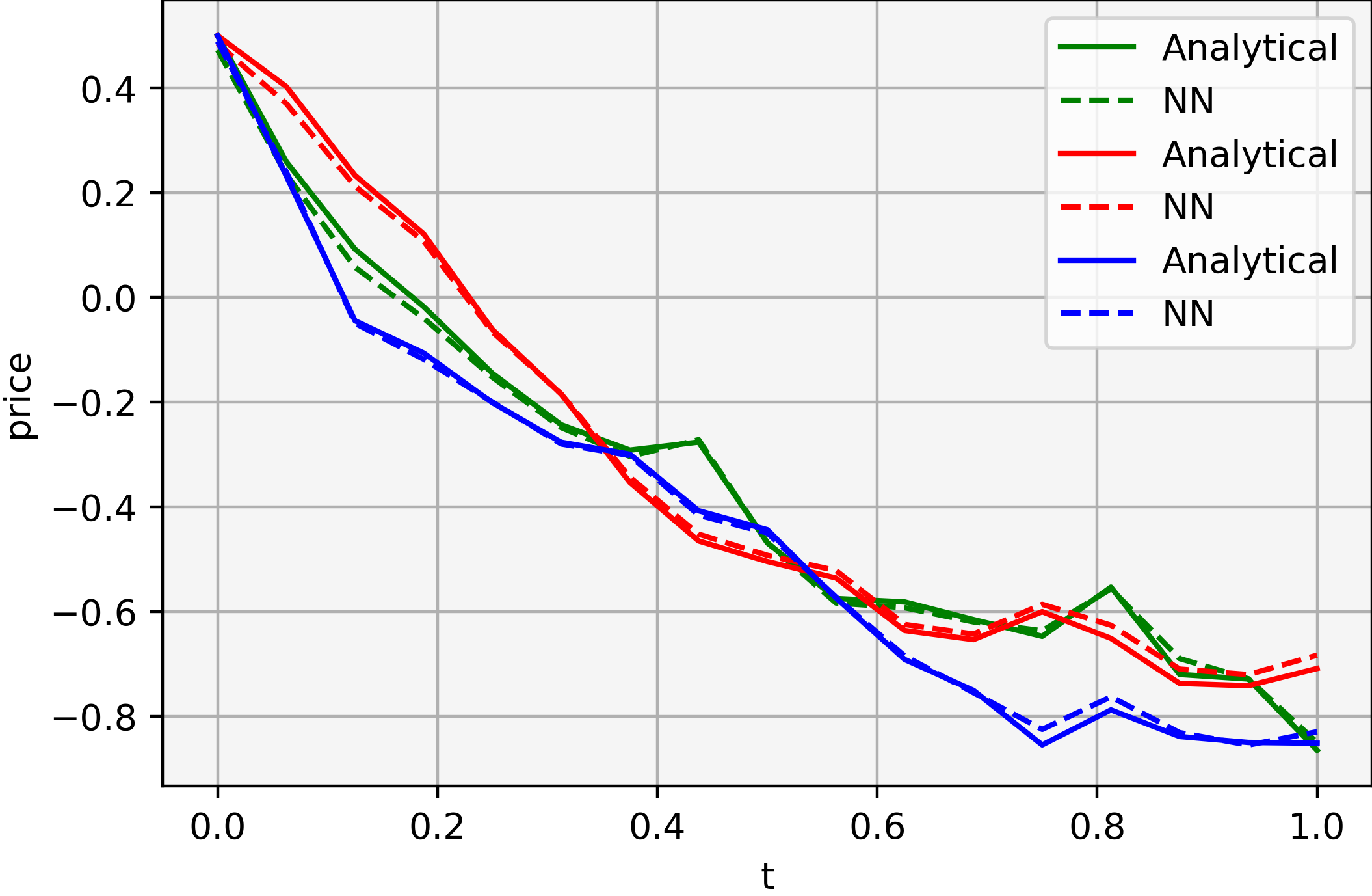
Figure 4: Stochastic price approx. (3 samples)

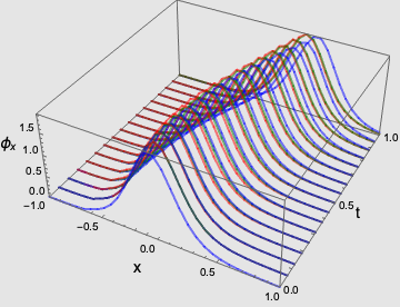
Figure 5: $m=\varphi_{x}$ approximation (3 samples)

VI Conclusions and future work

We developed a variational approach to price formation with common noise. This formulation, combined with machine learning techniques, provides an approach to solving infinite-dimensional MFGs. Future work should identify better network architectures and convergence results. A posteriori estimates would also be extremely interesting as they would provide a way to ensure the convergence.

VII Acknowledgments

The authors were supported by King Abdullah University of Science and Technology (KAUST) baseline funds and KAUST OSR-CRG2021-4674.

References

- [1] Y. Achdou, F. Camilli, and I. Capuzzo-Dolcetta. Mean field games: numerical methods for the planning problem. SIAM J. Control Optim., 50(1):77–109, 2012.
- [2] Y. Achdou and I. Capuzzo-Dolcetta. Mean field games: numerical methods. SIAM J. Numer. Anal., 48(3):1136–1162, 2010.
- [3] Y. Achdou, P. Cardaliaguet, F. Delarue, A. Porretta, and F. Santambrogio. Mean field games, volume 2281 of Lecture Notes in Mathematics. Springer, Cham; Centro Internazionale Matematico Estivo (C.I.M.E.), Florence, [2020] ©2020. Edited by Pierre Cardaliaguet and Alessio Porretta, Fondazione CIME/CIME Foundation Subseries.
- [4] R. Aid, A. Cosso, and H. Pham. Equilibrium price in intraday electricity markets, 2020.
- [5] R. Aïd, R. Dumitrescu, and P. Tankov. The entry and exit game in the electricity markets: A mean-field game approach. Journal of Dynamics & Games, 8(4):331–358, 2021.
- [6] C. Alasseur, I. Ben Taher, and A. Matoussi. An extended mean field game for storage in smart grids. Journal of Optimization Theory and Applications, 184(2):644–670, 2020.
- [7] C. Alasseur, L. Campi, R. Dumitrescu, and J. Zeng. Mfg model with a long-lived penalty at random jump times: application to demand side management for electricity contracts, 2021.
- [8] A. Alharbi, T. Bakaryan, R. Cabral, S. Campi, N. Christoffersen, P. Colusso, O. Costa, S. Duisembay, R. Ferreira, D. Gomes, S. Guo, J. Gutierrez-Pineda, P. Havor, M. Mascherpa, S. Portaro, R. Ribeiro, F. Rodriguez, J. Ruiz, F. Saleh, C. Strange, T. Tada, X. Yang, and Z. Wróblewska. A price model with finitely many agents. Bulletin of the Portuguese Mathematical Society, 2019.
- [9] Y. Ashrafyan, T. Bakaryan, D. Gomes, and J. Gutierrez. A duality approach to a price formation mfg model. 2021.
- [10] Y. Ashrafyan, T. Bakaryan, D. Gomes, and J. Gutierrez. A variational approach for price formation models in one dimension, 2022.
- [11] T. Bakaryan, R. Ferreira, and D. Gomes. A Potential Approach for Planning Mean-Field Games in One Dimension . Submitted to Communications on Pure and Applied Analysis, 2021.
- [12] T. Basar and R. Srikant. Revenue-maximizing pricing and capacity expansion in a many-users regime. In Proceedings.Twenty-First Annual Joint Conference of the IEEE Computer and Communications Societies, volume 1, pages 294–301 vol.1, 2002.
- [13] G. Csat’o, B. Dacorogna, and O. Kneuss. The Pullback Equation for Differential Forms. Progress in Nonlinear Differential Equations and their Applications. Birkhäuser/Springer, New York, 2012.
- [14] B. Djehiche, J. Barreiro-Gomez, and H. Tembine. Price Dynamics for Electricity in Smart Grid Via Mean-Field-Type Games. Dynamic Games and Applications, 10(4):798–818, December 2020.
- [15] O. Féron, P. Tankov, and L. Tinsi. Price Formation and Optimal Trading in Intraday Electricity Markets with a Major Player. Risks, 8(4):1–1, December 2020.
- [16] O. Féron, P. Tankov, and L. Tinsi. Price formation and optimal trading in intraday electricity markets, 2021.
- [17] M. Fujii and A. Takahashi. A Mean Field Game Approach to Equilibrium Pricing with Market Clearing Condition. Papers 2003.03035, arXiv.org, Mar. 2020.
- [18] M. Fujii and A. Takahashi. Equilibrium price formation with a major player and its mean field limit, 2021.
- [19] D. Gomes, J. Gutierrez, and R. Ribeiro. A random-supply Mean Field Game price model. arXiv e-prints, page arXiv:2109.01478, Sept. 2021.
- [20] D. Gomes, J. Gutierrez, and R. Ribeiro. A mean field game price model with noise. Math. Eng., 3(4):Paper No. 028, 14, 2021.
- [21] D. Gomes and J. Saúde. A Mean-Field Game Approach to Price Formation. Dyn. Games Appl., 11(1):29–53, 2021.
- [22] M. Huang, R. P. Malhamé, and P. E. Caines. Large population stochastic dynamic games: closed-loop McKean-Vlasov systems and the Nash certainty equivalence principle. Commun. Inf. Syst., 6(3):221–251, 2006.
- [23] J.-M. Lasry and P.-L. Lions. Jeux à champ moyen. I. Le cas stationnaire. C. R. Math. Acad. Sci. Paris, 343(9):619–625, 2006.
- [24] H. Shen and T. Basar. Pricing under information asymmetry for a large population of users. Telecommun. Syst., 47(1-2):123–136, 2011.
- [25] A. Shrivats, D. Firoozi, and S. Jaimungal. A Mean-Field Game Approach to Equilibrium Pricing, Optimal Generation, and Trading in Solar Renewable Energy Certificate Markets. Papers 2003.04938, arXiv.org, Mar. 2020.