Circuit Model Reduction with Scaled Relative Graphs

Abstract

Continued fractions are classical representations of complex objects (for example, real numbers) as sums and inverses of simpler objects (for example, integers). The analogy in linear circuit theory is a chain of series/parallel one-ports: the port behavior is a continued fraction containing the port behaviors of its elements. Truncating a continued fraction is a classical method of approximation, which corresponds to deleting the circuit elements furthest from the port. We apply this idea to chains of series/parallel one-ports composed of arbitrary nonlinear relations. This gives a model reduction method which automatically preserves properties such as incremental positivity. The Scaled Relative Graph (SRG) gives a graphical representation of the original and truncated port behaviors. The difference of these SRGs gives a bound on the approximation error, which is shown to be competitive with existing methods.

I Introduction

Continued fractions are classical in the theory of approximation [1], and are closely related to Padé approximants [2], which have had a broad impact in areas such as theoretical physics [3], fluid mechanics [4], and control theory [5, 6, 7, 8]. Continued fractions also have a long and rich history in linear circuit theory [9]. They have been used extensively for synthesis and approximation, beginning in the seminal works of Foster [10], Cauer [11], Bott, Duffin [12], and Kalman [5], among others. The Cauer normal forms for RC and RL circuits are continued fractions of transfer functions [9], and the truncation of a continued fraction corresponds to deleting elements from a series/parallel one-port. The nonlinear counterpart of this fruitful circle of ideas, however, is largely unexplored. In this context, this paper proposes the truncation of a “continued fraction” of nonlinear relations as a paradigm for model reduction of nonlinear series/parallel one-ports.

The aim of model reduction is to approximate a complex model by a simpler one, whilst retaining the important behavior. In particular, one may require that properties of the model (such as stability or passivity) are preserved by the approximation. For linear systems, the literature on the subject is vast, see, for example, [8] and references therein. In contrast, the problem is largely open for nonlinear systems. Some progress has been made in [13],  [14] and [15], and in the recent papers [16] and [17], the Lur’e structure is exploited to reduce a nonlinear model, while preserving incremental dissipativity properties. A nonlinear system is represented as a linear time invariant (LTI) state space model in feedback with a static nonlinearity. The LTI component is then approximated using standard methods, such as balanced truncation and Hankel norm approximation [8]. Although computationally effective, this procedure does not leverage the structure of the underlying physical system, and it is difficult, in general, to guarantee that the approximate system exhibits desired properties, such as positivity (a close relative of passivity [18, Lemma 2, p. 200]). In contrast, we propose that a system be modelled from the very beginning as an interconnection of physical components, and the system be approximated by deleting the components which are least important. Properties which are preserved by physical interconnection, such as positivity [18, $\S 5$, Chap. 6], are then naturally retained in the approximate system. The choice of electrical terminology is purely a matter of preference: series/parallel electrical circuits have analogies in domains such as mechanics, hydraulics and thermodynamics [19, 20].

This paper proposes the Scaled Relative Graph (SRG) as a tool for quantifying the errors introduced by an approximation. The SRG has recently been introduced in the theory of convex optimization [21], and allows simple, graphical proofs of algorithm convergence, and the derivation of tight convergence bounds [22]. The SRG gives a graphical representation of the incremental behavior of a nonlinear operator, and generalizes the Nyquist diagram of an LTI transfer function [23]. Interconnections of operators correspond to graphical combinations of their SRGs [21], and applying this graphical algebra to the study of feedback systems gives rise to a nonlinear Nyquist criterion, which generalizes many existing results on incremental input/output stability [23, 24]. Properties such as incremental gain and incremental positivity can be read directly from the SRG, and as such the SRG may be used to measure the error introduced in such quantities. Plotting an SRG for the error system, that is, the difference between a system and its approximation, allows us to bound the incremental gain from input to approximation error. This bound is shown to compare favourably with other bounds in the literature.

We begin this paper in Section II with a motivating example, which illustrates the main ideas. We then define the model class and propose a truncation procedure in Section III. Section IV introduces the SRG, and how it may be used to certify approximation error bounds. Equipped with these tools, we revisit the example circuit in Section V, and compare our method with the method described in [25]. Section VI concludes the paper with a summary of our main results, and poses open questions for future research.

II A motivating example

The running example of this paper is the circuit illustrated in Figure 1. $G_{RC}$ is the admittance of an LTI RC filter, and $R$ is an arbitrary nonlinear resistor $v=R(i)$ which, for all $v_{1},v_{2},i_{1},i_{2}$, satisfies the incremental sector bound

$$\mu\Delta i^{2}\leq\Delta i\Delta v\leq\lambda\Delta i^{2},$$ (1)

for some $0\leq\mu\leq\lambda$, where $\Delta i=i_{1}-i_{2}$ and $\Delta v=v_{1}-v_{2}$.

Figure 1: A nonlinear lattice circuit, configured as a one-port.

The circuit consists of a chain $n$ repeated three element units, and an additional RC filter at the port. A first attempt at approximating the circuit might simply be to remove the units furthest from the port. This corresponds to truncating a “continued fraction” in the circuit elements (to be made precise in Section III). A better method might be to only remove the capacitors furthest from the port, and resolve the remaining (linear and nonlinear) resistors into a single nonlinear resistor. This gives the same continued fraction truncation, with an additional nonlinear resistance. If $R$ is LTI, one can show that the approximation error is always bounded by the $H$ norm of the original circuit’s transfer function [26]. We generalize this result to the case where $R$ is nonlinear, using SRGs.

The SRG of a circuit of length $n$ is shown in Figure 2. The value $\lambda_{n}$ (defined in Section V) bounds the incremental secant gain [27, $\S$2] of the circuit, and we will show that it also bounds the gain in the error, $\norm{v-\hat{v}}/\norm{i}$, where $i$ is an input current, $v$ is the output voltage of the original circuit and $\hat{v}$ is the output voltage of any circuit with the last $r<n$ capacitors removed.

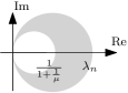
Figure 2: SRG for the current to voltage relation of the circuit of Figure 1.

III Truncating series/parallel one-port circuits

III-A Circuit elements as relations

Let $L_{2}$ denote the set of finite energy signals $u:[0,\infty)\to\mathbb{R}$ such that ${\int_{0}|u^{2}(t)|\mathrm{d}t<\infty.}$ The inner product on $L_{2}$ is defined by

$$\bra{u}\ket{y}\coloneqq\int_{0}u(t)y(t)\mathrm{d}t,$$

which induces the norm $\norm{u}\coloneqq\sqrt{\bra{u}\ket{u}}$.

We consider circuits formed by the parallel and series interconnection of one-port elements. A one-port has two terminals, across which a voltage $v$ is measured, and through which a current $i$ flows. We assume that these currents and voltages belong to $L_{2}$, and a one-port $R$ is described by a relation on $L_{2}$, that is, a set $R\subseteq L_{2}\times L_{2}$ of ordered voltage/current pairs. If a one-port is described by a relation from voltage to current, it is an admittance, and if a one-port is described by a relation from current to voltage, it is an impedance. If $(u,y)\in R$, we write $y\in R(u)$.

The usual operations on functions can be extended to relations:

$$S^{-1} = \{(y,u)\;|\;y\in S(u)\}$$

$$S+R = \{(x,y+z)\;|\;(x,y)\in S,\;(x,z)\in R\}$$

$$SR = \{(x,z)\;|\;\exists\,y\text{ s.t. }(x,y)\in R,\;(y,z)\in S\}.$$

The relational inverse always exists, but is not an inverse in the usual sense – in particular, it is in general not the case that $R^{-1}R=I$. If, however, $R$ is an invertible function, its functional inverse coincides with its relational inverse, so the notation $R^{-1}$ is not ambiguous. If $R$ is an impedance, mapping $i$ to $v$, then $R^{-1}$ is an admittance, mapping $v$ to $i$.

Definition 1.

A relation $R$ on $L_{2}$, mapping $u$ to $y$, is said to be

1. incrementally positive (or monotone) if $\bra{u_{1}-u_{2}}\ket{y_{1}-y_{2}}\geq 0$ for all $u_{1},u_{2},y_{1}\in R(u_{1}),y_{2}\in R(u_{2})$;

2. $\mu$-input strictly incrementally positive (or $\mu$-coercive) if $\bra{u_{1}-u_{2}}\ket{y_{1}-y_{2}}\geq\mu\norm{u_{1}-u_{2}}^{2}$ for all $u_{1},u_{2},y_{1}\in R(u_{1}),y_{2}\in R(u_{2})$;

3. $1/\gamma$-output strictly incrementally positive (or $1/\gamma$-cocoercive) if $\gamma\bra{u_{1}-u_{2}}\ket{y_{1}-y_{2}}\geq\norm{y_{1}-y_{2}}^{2}$ for all $u_{1},u_{2},y_{1}\in R(u_{1}),y_{2}\in R(u_{2})$. $\gamma$ is called the incremental secant gain.

4. $R$ is said to have an incremental gain bound (or Lipschitz constant) of $\lambda$ if $\norm{y_{1}-y_{2}}\leq\lambda\norm{u_{1}-u_{2}}$ for all $u_{1},u_{2},y_{1}\in R(u_{1}),y_{2}\in R(u_{2})$.

The incremental secant gain of a system is also an incremental gain bound.

Incremental positivity is closely related to incremental passivity – the two are equivalent for causal operators (this follows from an easy adaptation of the proof of [18, Lemma 2, p. 200]). Examples of incrementally positive circuit elements include resistors with nondecreasing $i-v$ characteristics and LTI capacitors and inductors [28].

III-B Series/parallel one-port circuits

A series interconnection of two impedances $R_{1}$ and $R_{2}$ defines a new one-port impedance, $R_{1}+R_{2}$:

$$v\in R_{1}(i)+R_{2}(i).$$

Likewise, the parallel interconnection of two admittances $G_{1}$ and $G_{2}$ defines the one-port admittance $G_{1}+G_{2}$:

$$i\in G_{1}(v)+G_{2}(v).$$

Interconnecting an impedance and an admittance, either in series or in parallel, requires one of the relations to be inverted. We will assume throughout this paper that any relations which are added have compatible domains. For a circuit-theoretic interpretation of this assumption, see [28, Thm. 2].

These interconnection rules give rise to the class of one-port circuits consisting of arbitrary series/parallel interconnections, which have the general form shown in Figure 3 (allowing admittances to be open circuits, $\{(v,0)\;|\;v\in\mathbb{R}\}$, and impedances to be short circuits, $\{(i,0)\;|\;i\in\mathbb{R}\}$).

Figure 3: Circuit structure with nested series and parallel interconnections. $R_{n}$ represents an impedance, $G_{n}$ represents an admittance.

The $v-i$ relation of this general circuit is given by

$$v_{0} = (R_{0}+(G_{0}+(\ldots+(R_{n-1}+R_{n})^{-1}\ldots)^{-1})^{-1})(i_{0}).$$

Note that this form generalizes a continued fraction of transfer functions: when all the elements $R_{j}$ and $G_{j}$ are LTI, taking the Laplace transform gives

$$v_{0}(s)=R_{0}(s)+\cfrac{1}{G_{0}(s)+\cfrac{1}{\ldots+\cfrac{1}{R_{n-1}(s)+R_{n}(s)}}}\,i_{0}(s).$$

When every element is incrementally positive, such circuits are closely related to the splitting algorithms of monotone operator theory, and may be solved efficiently using the recently introduced class of nested splitting algorithms [28].

III-C Truncated approximate circuits

Consider the problem of approximating the one-port circuit in Figure 3, whose port behavior is given by $v_{0}=C(i_{0})$, by a simpler one-port. A natural solution is to delete the circuit elements furthest from the port terminals, as they contribute the least to the port behavior of the circuit. This gives a truncated circuit $\hat{C}$ with $i-v$ relation, defined by

$$\hat{v}_{0}=(R_{0}+(G_{0}+(\ldots+(R_{r-1}+R_{r})^{-1}\ldots)^{-1})^{-1})(i_{0}),$$

where $r<n$. This procedure corresponds to truncating the continued fraction of the circuit. The relation from current to voltage has been chosen arbitrarily, and it is straightforward to verify that the truncation of $C^{-1}$ is $\hat{C}^{-1}$. We will also consider the case where the final impedance $R_{r}$ is modified to some $\hat{R}_{r}$ – for example, the lumped resistance which remains when only capacitors are removed from the circuit in Figure 1.

In the case that all the circuit elements $R_{j}$, $G_{j}$ are incrementally positive, both the original and truncated circuits are automatically incrementally positive – this follows from the preservation of incremental positivity under series and parallel interconnections [28, Prop. 1]. In the case that the circuit elements have stronger positivity properties, these are also preserved in the truncated circuit, as shown in the following proposition.

Proposition 1.

Consider the circuit in Figure 3. Suppose that each admittance $G_{j}$ is input-strictly incrementally positive, and each impedance $R_{j}$ is output-strictly incrementally positive. Then the circuit is input-strictly incrementally positive from voltage to current, and output-strictly incrementally positive from current to voltage.

Proof.

The proof follows from induction, and the following basic results (see, for example, [29, Chap. 2]). Let $A$ and $B$ be relations on an arbitrary Hilbert space. Then:

1. If $A$ and $B$ are input-strictly incrementally positive, then $A+B$ is input-strictly incrementally positive.

2. If $A$ and $B$ are output-strictly incrementally positive, then $A+B$ is output-strictly incrementally positive.

3. If $A$ is input-strictly incrementally positive, $A^{-1}$ is output-strictly incrementally positive.

4. If $A$ is output-strictly incrementally positive, $A^{-1}$ is input-strictly incrementally positive.∎

As the series/parallel structure of a circuit is preserved as elements are removed, Proposition 1 shows that truncation preserves strict incremental positivity. In the following section, we will develop several numerical estimates of the accuracy of an approximation, using the circuit’s SRG.

IV Graphical truncation errors

We begin this section with a brief overview of the theory of SRGs. For a full treatment, we refer the reader to [21].

IV-A Scaled Relative Graphs

The SRG of an operator is a region in the extended complex plane from which the dynamic properties of the operator can be easily read. We define the SRG formally as follows.

The angle between $u,y\in L_{2}$ is defined as

$$\angle(u,y)\coloneqq\acos\frac{\bra{u}\ket{y}}{\norm{u}\norm{y}}\in[0,\pi).$$

Let $R\subseteq L_{2}\times L_{2}$. Given $u_{1},u_{2}\in L_{2}$, $u_{1}\neq u_{2}$, we define the set of complex numbers $z_{R}(u_{1},u_{2})$ by

$$\left\{\frac{\norm{y_{1}-y_{2}}}{\norm{u_{1}-u_{2}}}e^{\pm j\angle(u_{1}-u_{2},y_{1}-y_{2})}\middle|\;y_{1}\in R(u_{1}),y_{2}\in R(u_{2})\right\}.$$

If $u_{1}=u_{2}$ and there exist corresponding outputs $y_{1}\in R(u_{1}),y_{2}\in R(u_{2}),y_{1}\neq y_{2}$, then $z_{R}(u_{1},u_{2})$ is defined to be $\{\infty\}$. If $R$ is single valued at $u_{1}$, $z_{R}(u_{1},u_{1})$ is the empty set.

The Scaled Relative Graph (SRG) of $R$ over $L_{2}$ is then given by

$$\operatorname{SRG}_{\,}({R})\coloneqq\tbigcup\slimits@_{u_{1},u_{2}\in\,L_{2}}z_{R}(u_{1},u_{2}).$$

Proposition 2.

The SRG of a relation belongs to one of the regions illustrated below if and only if the relation obeys the corresponding input/output property. Clockwise from top left: finite incremental gain, $1/\gamma$-output strict incremental positivity, $\mu$-input strict incremental positivity.

IV-B SRGs of series/parallel one-ports

Connecting elements in series and parallel involves adding and inverting their relations. In this section, we describe the corresponding graphical operations on their SRGs.

If $C,D\subseteq\mathbb{C}$, we define the operation $C+D$ to be the Minkowski sum of $C$ and $D$, that is,

$$C+D\coloneqq\{c+d\,|\,c\in C,d\in D\}.$$

We define inversion in the extended complex plane by $re^{j\omega}\mapsto(1/r)e^{j\omega}$. This maps points outside the unit circle to the inside, and vice versa. The points $0$ and are exchanged under inversion. The complex conjugate would normally be taken; this is left out for convenience, and has no effect as the SRG is symmetric about the real axis.

Define the line segment between $z_{1},z_{2}\in\mathbb{C}$ as $[z_{1},z_{2}]\coloneqq\{\alpha z_{1}+(1-\alpha)z_{2}\,|\,\alpha\in[0,1]\}$. A region $G\subseteq\mathbb{C}$ is said to satisfy the chord property if $z\in G$ implies $[z,\bar{z}]\subseteq G$. If $A$ is a relation, we denote by $\overline{\operatorname{SRG}_{\,}({A})}$ any region in $\mathbb{C}$ such that $\operatorname{SRG}_{\,}({A})\subseteq\overline{\operatorname{SRG}_{\,}({A})}$ and $\overline{\operatorname{SRG}_{\,}({A})}$ satisfies the chord property.

Proposition 3.

If $A$ is an operator, then $\operatorname{SRG}_{\,}({-A})=-\operatorname{SRG}_{\,}({A})$.

Proposition 4.

If $A$ is an operator, then $\operatorname{SRG}_{\,}({A^{-1}})=(\operatorname{SRG}_{\,}({A}))^{-1}$.

Proposition 5.

Let $A$ and $B$ be relations whose SRGs are bounded. Then $\operatorname{SRG}_{\,}({A+B})\subseteq\operatorname{SRG}_{\,}({A})+\overline{\operatorname{SRG}_{\,}({B})}$.

Unbounded SRGs can be allowed by setting $\operatorname{SRG}_{\,}({A+B})=\{\infty\}$ if $\operatorname{SRG}_{\,}({A})=\varnothing$ and $\infty\in\operatorname{SRG}_{\,}({B})$.

IV-C Graphical truncation errors for series/parallel one-ports

To evaluate the error introduced by truncating a circuit, we can compute a bounding SRG for the error relation, $C-\hat{C}$, which maps $u$ to $e\coloneqq y-\hat{y}$. It follows from Proposition 2 that the maximum modulus of $\operatorname{SRG}_{\,}({C-\hat{C}})$ bounds the incremental error gain,

$$\sup_{u_{1},u_{2}\in L_{2},u_{1}\neq u_{2}}\frac{\norm{e_{1}-e_{2}}}{\norm{u_{1}-u_{2}}}.$$

If this quantity is bounded, the error relation is continuous on $L_{2}$: small changes in the input result in small changes in the error. Under the assumption that $0\in C(0)$ and $0\in\hat{C}(0)$, the incremental error gain, in turn, bounds

$$\sup_{u\in L_{2},\norm{u}\neq 0}\frac{\norm{y-\hat{y}}}{\norm{u}}.$$

If this quantity is bounded, the error relation is bounded on $L_{2}$: bounded inputs result in bounded errors.

Using the SRGs of the original and truncated circuits, we can furthermore measure the error in various dynamic properties, such as incremental gain and positivity. Figure 4, for example, shows how the error in the secant gain can be measured from the original and truncated SRGs.

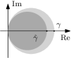
Figure 4: Suppose the light grey region bounds the SRG of the original circuit, and the dark grey region bounds the SRG of the truncated circuit. The original circuit has a secant gain of $\gamma$, and the truncated circuit has a secant gain of $\hat{\gamma}$. The error $\gamma-\hat{\gamma}$ in the truncated secant gain is the distance between the two marked points on the real axis.

V Example revisited

Armed with the graphical tools of the previous section, we revisit the example of Section II. We begin by deriving an SRG for the circuit in Figure 1, for an arbitrary number of units $n$. Recall that $R$ is an arbitrary nonlinear resistor which satisfies the incremental sector bound (1), and suppose the capacitor and linear resistor both have unit value, $C=G=1$. The SRGs of $R$ and $G_{RC}$ are illustrated below (following [23, Thm. 4, Prop. 9]).

We then apply the SRG sum and inversion rules (Propositions 5 and 4) to obtain the SRG for the $i-v$ relation of a circuit with $n=1$, shown below (incidentally, we also obtain an SRG for the $v-i$ relation).

Carrying on with this procedure, we obtain the following SRG for a circuit with $n$ units.

$\lambda_{n}$ is defined recursively by

$$\lambda_{n} = \begin{cases}\frac{1}{1+\frac{1}{\lambda+1}}&n=1\\ \frac{1}{1+\frac{1}{\lambda+\lambda_{n-1}}}&n>1.\end{cases}$$

Repeating this procedure for a circuit $\hat{C}$ with the last $n-r$ capacitors removed produces an identical SRG. We can compute an SRG for the error relation $C-\hat{C}$ by subtracting $\operatorname{SRG}_{\,}({\hat{C}})$ from $\operatorname{SRG}_{\,}({C})$. This is bounded by the disc illustrated below.

It follows from Proposition 2 that the error relation, which maps $i\coloneqq i_{0}$ to $e\coloneqq v_{0}-\hat{v}_{0}$, has an incremental gain bound of $\lambda_{n}$:

$$\sup_{i\in L_{2},\norm{i}\neq 0}\frac{\norm{v_{0}-\hat{v}_{0}}}{\norm{i}} \sup_{i_{1},i_{2}\in L_{2},i_{1}\neq i_{2}}\frac{\norm{e_{1}-e_{2}}}{\norm{i_{1}-i_{2}}}\leq\lambda_{n}.$$

This bound depends only on $\lambda$ and $n$, and approaches a constant as $n\to\infty$.

Comparing the SRGs of $C$ and $\hat{C}$ shows that both circuits are output-strictly incrementally passive, with an incremental secant gain of $\lambda_{n}$.

By way of comparison, applying the balanced truncation method presented in [25], with $R^{-1}(v)=\tanh(v)+v$, results in a pure truncation of the continued fraction of the circuit, by removing $n-r$ repeated units, and gives an error bound

$$\sup_{i\in L_{2},\norm{i}\neq 0}\frac{\norm{v_{0}-\hat{v}_{0}}}{\norm{i}} \frac{n-r}{(1-\gamma)^{2}},$$

where $\gamma=l\lambda$, and $l$ is the largest eigenvalue of the $n\times n$ matrix

$$\begin{pmatrix}-2&1&0&\ldots&0\\ 1&-2&1&\ldots&0\\ 0&1&-2&\ldots&0\\ \@vdots&\@vdots&\@vdots&\ddots&\@vdots\\ 0&0&0&\ldots&0\end{pmatrix}.$$

Note that the eigenvalue $l$ converges to $4$ as $n\to\infty$. This bound is tighter than $\lambda_{n}$ for small $n$, but diverges as $n\to\infty$. The two bounds are plotted in Figure 5.

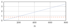
Figure 5: Maximum modulus of $\operatorname{SRG}_{\,}({C-\hat{C}})$ (orange, dashed) and the error bound obtained from [25] (blue, dotted). The truncated circuit has length $r=3$, and $\lambda=2$.

The performance of the two truncations is compared in Figure 6, for an input of $i_{0}(t)=\sin(t)$, and Figure 7, for an input of $i_{0}(t)=\sin(2t)$. Both simulations use an initial condition of $1$ V across each capacitor. The original circuit length is $n=50$, and the truncated circuit length is $r=3$. For the method we present here, the $n-r$ nonlinear resistors which remain after the capacitors are removed are approximated by piecewise-linear functions. The method we present here has lower error in both cases, both in absolute magnitude and in phase shift.

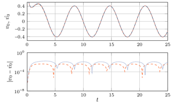
Figure 6: Top: Time history of the output of the circuit in Figure 1 with $n=50$ (solid black) and those of the reduced order models of order ${r=3}$ using the method we present here (dashed orange) and the differential balanced truncation method of [25] (dotted blue). The initial condition is $1$ V across each capacitor, and the input is $i_{0}(t)=\sin(t)$. Bottom: Time history of the corresponding output errors in absolute value (logarithmic scale).

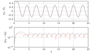
Figure 7: The same experiment as Figure 6, with $i_{0}(t)=\sin(2t)$.

In contrast with the balanced truncation method of [25], $R$ can be non-differentiable and non-invertible (for example, a unit ideal saturation), does not have to be a function (for example, an ideal diode) and need not be time-invariant; the element closest to the port can be linear or nonlinear; and the voltage to current relation is just as easily analysed as the current to voltage relation.

VI Conclusions

This paper explores a simple method for approximating systems which are modelled as the port behavior of a series/parallel interconnection of nonlinear relations. Deleting the elements furthest from the port corresponds to truncating a continued fraction. Resistances can be left in place and lumped into a single element. This procedure automatically guarantees the preservation of properties such as incremental positivity (regular, input-strict and output-strict) and finite incremental gain.

The error introduced by the truncation can be evaluated using the SRGs of the original and truncated systems. Distances between the two SRGs correspond to errors in quantities such as the incremental secant gain. Furthermore, an SRG can be computed for the error relation, and this gives a bound on the incremental gain from the input to the truncation error.

A natural open question concerns the generality of the series/parallel structure: when can a system be modelled as a series/parallel one-port? This is a nonlinear version of one of the earliest questions in circuit theory: when can a transfer function be realised as the port behavior of an RLC one-port? This question arose in the work of Foster [10], Cauer [11], and Brune [30], and a constructive solution was provided by Bott and Duffin [12]. The Bott-Duffin construction is still the subject of active research [31, 32]. We leave the equivalent nonlinear construction as a question for future research.

References

- [1] W.. Jones and W.. Thron “Continued fractions: Analytic theory and applications” Cambridge, U.K.: Cambridge Univ. Press, 1984
- [2] G.. Baker and P. Graves-Morris “Padé approximants (2nd edition)” Cambridge, U.K.: Cambridge Univ. Press, 1996
- [3] G.. Baker and J.. Gammel “The Padé approximant in theoretical physics” New York, NY, USA: Academic Press, 1970
- [4] Henri Cabannes “Padé approximants method and its applications to mechanics” Heidelberg, Germany: Springer-Verlag, 1976
- [5] R.. Kalman “On partial realizations, transfer functions and canonical forms” In Acta Polytechnica Scandinavica 31, 1979, pp. 9–32
- [6] A. Antoulas “On recursiveness and related topics in linear systems” In IEEE Transactions on Automatic Control 31.12, 1986, pp. 1121–1135 DOI: 10.1109/TAC.1986.1104191
- [7] A. Bultheel and B. De Moor “Rational approximation in linear systems and control” In J. Comp. Appl. Math. 121.1-2, 2000, pp. 355–378
- [8] A.. Antoulas “Approximation of large-scale dynamical systems” Philadelphia, PA, USA: SIAM, 2005
- [9] R.. Newcomb “Linear multiport synthesis” NEw York, NY, USA: McGraw-Hill, 1966
- [10] Ronald M. Foster “A Reactance Theorem” In Bell System Technical Journal 3.2, 1924, pp. 259–267 DOI: 10.1002/j.1538-7305.1924.tb01358.x
- [11] Wilhelm Cauer “Die Verwirklichung von Wechselstromwiderständen Vorgeschriebener Frequenzabhängigkeit” In Archiv für Elektrotechnik 17.4, 1926, pp. 355–388 DOI: 10.1007/BF01662000
- [12] R. Bott and R.. Duffin “Impedance Synthesis without Use of Transformers” In Journal of Applied Physics 20.8, 1949, pp. 816–816 DOI: 10.1063/1.1698532
- [13] Jacqueline Maria Aleida Scherpen “Balancing for nonlinear systems” In Systems & Control Letters 21.2 Elsevier, 1993, pp. 143–153
- [14] Alessandro Astolfi “Model reduction by moment matching for linear and nonlinear systems” In IEEE Transactions on Automatic Control 55.10 IEEE, 2010, pp. 2321–2336
- [15] A. Padoan “Model reduction by least squares moment matching for linear and nonlinear systems” under review In IEEE Transactions on Automatic Control, 2021
- [16] Bart Besselink, Nathan Wouw and Henk Nijmeijer “Model reduction for nonlinear systems with incremental gain or passivity properties” In Automatica 49.4 Elsevier, 2013, pp. 861–872
- [17] A. Padoan, F. Forni and R. Sepulchre “Model reduction of dominant feedback systems” In Automatica 130.109695, 2021, pp. 1–8 DOI: 10.1016/j.automatica.2021.109695
- [18] Charles A. Desoer and Mathukumalli Vidyasagar “Feedback Systems: Input–Output Properties” Elsevier, 1975 DOI: 10.1016/b978-0-12-212050-3.x5001-4
- [19] M.. Smith “Synthesis of Mechanical Networks: The Inerter” In IEEE Transactions on Automatic Control 47.10, 2002, pp. 1648–1662 DOI: 10.1109/tac.2002.803532
- [20] Arjan Schaft and Dimitri Jeltsema “Port-Hamiltonian Systems Theory: An Introductory Overview” In Foundations and Trends in Systems and Control 1.2-3, 2014, pp. 173–378 DOI: 10.1561/2600000002
- [21] Ernest K. Ryu, Robert Hannah and Wotao Yin “Scaled Relative Graphs: Nonexpansive Operators via 2D Euclidean Geometry” In Mathematical Programming, 2021 DOI: 10.1007/s10107-021-01639-w
- [22] Xinmeng Huang, Ernest K. Ryu and Wotao Yin “Tight Coefficients of Averaged Operators via Scaled Relative Graph”, 2020 arXiv:1912.01593 [math]
- [23] Thomas Chaffey, Fulvio Forni and Rodolphe Sepulchre “Graphical Nonlinear System Analysis”, 2021 arXiv:2107.11272 [cs, eess, math]
- [24] Thomas Chaffey “A Rolled-off Passivity Theorem” In Systems & Control Letters 162, 2022, pp. 105198 DOI: 10.1016/j.sysconle.2022.105198
- [25] Bart Besselink, Nathan Wouw, Jacquelien M.. Scherpen and Henk Nijmeijer “Model Reduction for Nonlinear Systems by Incremental Balanced Truncation” In IEEE Transactions on Automatic Control 59.10, 2014, pp. 2739–2753 DOI: 10.1109/TAC.2014.2326548
- [26] B. Srinivasan and P. Myszkorowski “Model Reduction of Systems with Zeros Interlacing the Poles” In Systems & Control Letters 30.1, 1997, pp. 19–24 DOI: 10.1016/S0167-6911(96)00072-2
- [27] Eduardo D. Sontag “Passivity Gains and the “Secant Condition” for Stability” In Systems & Control Letters 55.3, 2006, pp. 177–183 DOI: 10.1016/j.sysconle.2005.06.010
- [28] Thomas Chaffey and Rodolphe Sepulchre “Monotone One-Port Circuits”, 2021 arXiv:2111.15407 [cs, eess, math]
- [29] Ernest K. Ryu and Wotao Yin “Large-Scale Convex Optimization via Monotone Operators”, 2022
- [30] Otto Brune “Synthesis of a Finite Two-Terminal Network Whose Driving-Point Impedance Is a Prescribed Function of Frequency”, 1931
- [31] Timothy H. Hughes and Malcolm C. Smith “On the Minimality and Uniqueness of the Bott–Duffin Realization Procedure” In IEEE Transactions on Automatic Control 59.7, 2014, pp. 1858–1873 DOI: 10.1109/TAC.2014.2312471
- [32] Timothy H. Hughes “Why RLC Realizations of Certain Impedances Need Many More Energy Storage Elements Than Expected” In IEEE Transactions on Automatic Control 62.9, 2017, pp. 4333–4346 DOI: 10.1109/TAC.2017.2667585