Compact-to-Dendritic Transition in the Reactive Deposition of Brownian Particles

Abstract

When Brownian particles—such as ions, colloids, or misfolded proteins—deposit onto a reactive cluster, the cluster undergoes a transition from a compact to a dendritic morphology. Continuum modeling reveals that the critical radius for this compact-to-dendritic (CTD) transition should be proportional to the particle diffusivity divided by the surface reaction rate. However, previous studies have had limited success verifying that the same scaling arises in the continuum limit of a particle-based deposition model. This discrepancy suggests that the continuum model may be missing part of the microscopic dendrite formation mechanism, a concerning hypothesis given that similar models are commonly used to study dendritic growth in electrodeposition and lithium metal batteries. To clarify the accuracy of such models, we reexamine the particle-based CTD transition using larger system sizes, up to hundreds of millions of particles in some cases, and an improved paradigm for the surface reaction. Specifically, this paradigm allows us to converge our simulations and to work in terms of experimentally accessible parameters. With these methods, we show that in both two and three dimensions, the behavior of the critical radius is consistent with the scaling of the continuum model. Our results help unify the particle-based and continuum views of the CTD transition. In each of these cases, dendrites emerge when particles can no longer diffuse around the cluster within the characteristic reaction timescale. Consequently, this work implies that continuum methods can effectively capture the microscopic physics of dendritic deposition.

I Introduction

Many systems that display dendritic growth consist of diffusive particles that deposit onto a reactive surface. Examples include colloidal aggregation, amyloid formation, and electrodeposition [1, 2, 3]. One way to understand these systems is by studying idealized models of reactive deposition [4, 5, 6, 7, 8, 9]. These models show that dendrites emerge due to a feedback loop. Incoming particles preferentially attach to the bumps of a reactive surface before they have time to diffuse into the valleys [10, 4]. The preferential deposition causes the bumps to grow faster than the rest of the surface, which exacerbates the preferential deposition, and so on.

In idealized models, the dendritic feedback loop also produces a deeper phenomenology. The thickness of the dendritic branches decreases as the rate of the surface reaction increases [4, 9]. This relationship is significant because it qualitatively matches what is observed in electrodeposition experiments [3]. Understanding branch thickness in idealized models can thus help clarify the mechanism of dendrite formation in a number of electrodeposition-based applications like batteries. Currently, dendrite formation in lithium-ion and next-generation alkali metal batteries is one of the primary sources of cell failure as it can deplete the working metal and the electrolyte, and create catastrophic short circuits [11, 12, 13].

In this work, we investigate the factors that determine dendritic branch thickness in idealized models specifically through the lens of the compact-to-dendritic (CTD) transition. This transition occurs when a small, compact cluster is embedded in a concentration field of reactive particles that cause it to grow outwards in all directions [4, 5, 6, 7, 8]. While at first, the cluster continues to display a compact morphology, upon reaching a critical radius, it splits into a characteristic dendritic pattern [14]. Illustrations of the growth process for two and three-dimensional deposition are shown in Fig. 1. Since the critical radius sets the resulting dendritic branch thickness, the CTD transition offers a convenient way to study the branch structure of the large length-scale dendritic morphology.

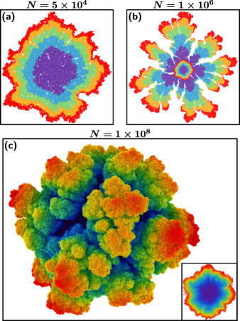
Figure 1: The compact-to-dendritic transition for discrete deposition at $\log_{10}\mathrm{Da}=-2.12$. Panels (a) and (b) illustrate the two-dimensional deposition process. The $N$ particles in these panels are rendered with a radius twice that of the actual radius for clarity. The $i$th band of color moving outwards from the center corresponds to the structure after $iN/5$ particles have been deposited. (a) Initially, the cluster displays a compact morphology. (b) However, upon reaching a critical radius, it spontaneously forms dendritic branches. (c) During three-dimensional deposition, a similar dendritic morphology emerges at large length scales. Here, particles are colored based on their distance from the origin. The inset shows a two-dimensional slice through the initial compact cluster, $N=1\times 10^{6}$, with a continuous gradient color scheme based on the deposition order.

Unfortunately, understanding this transition has proven to be challenging. Previous studies attempted to analyze the growing cluster by comparing the behavior of two related models of the deposition dynamics, a discrete model and a continuum model [4]. These models differ based on how they represent the concentration field that surrounds the cluster. In the discrete model, particles in the field are represented explicitly, and the cluster grows particle-by-particle. In contrast, in the continuum model, the concentration field itself is taken to be fundamental. Instead of growing particle-by-particle, the cluster grows outwards at all points simultaneously with a velocity proportional to the continuum flux.

The CTD transition in the continuum model can be treated analytically. A linear stability analysis reveals that for two and three-dimensional growth, the critical radius $R_{c}$ scales as

$$R_{c}\sim D/k,$$ (1)

where $D$ is the diffusion constant and $k$ is the surface reaction rate constant [4, 15, 16]. We will show that $D/k$ scaling is associated with a simple dendrite formation mechanism.

In comparison, the CTD transition in the discrete model is significantly more difficult to characterize. The behavior of this transition depends on the parameters of the deposition process through the dimensionless Damköhler number

$$\mathrm{Da}=\frac{ka}{D},$$ (2)

where $a$ is the particle radius. Physically, $\mathrm{Da}$ quantifies the relative rate of reaction versus diffusion in the system. In the limit as the reaction becomes infinitely fast, $\mathrm{Da}\to\infty$, the model approaches diffusion-limited aggregation (DLA). That is, particles begin to deposit as soon as they touch the cluster [17, 4]. As a result, the critical radius for the CTD transition tends towards zero, and the cluster immediately forms dendritic branches that are a single particle thick.

The limit $\mathrm{Da}\to 0$, in contrast, yields a nontrivial critical radius. This limit corresponds to making the surface reaction infinitely slow. Alternatively, $\mathrm{Da}\to 0$ can be thought of as the continuum limit since it can be reached by taking the particle radius $a$ to zero at fixed values of $k$ and $D$. In either view, when $\mathrm{Da}\to 0$, $R_{c}$ is expected to converge to the following power-law form based on dimensional analysis [18, 19]

$$\frac{kR_{c}}{D}\sim\mathrm{Da}^{\gamma}.$$ (3)

Here, $\gamma$ is an unknown scaling exponent that encodes the mechanistic details of CTD transition. This exponent plays a central role in the rest of this article.

Due to its mechanistic importance, a number of authors have previously analyzed $\gamma$ [4, 6, 8]. In particular, Witten and Sander hypothesized that the continuum limit of the discrete model (3) should reproduce the $D/k$ scaling of the continuum model (1) [4]. Their reasoning implies that, in two and three dimensions, $\gamma$ should be equal to zero.

However, the $\gamma=0$ hypothesis has received only limited empirical support. Refs. 6 and 8 calculated $\gamma$ using lattice-based and off-lattice 2D Brownian dynamics simulations and obtained estimates of $-0.2$ and $-0.25\pm 0.3$, respectively [20]. In the latter case, $\gamma=0$ is included at the edge of the error bars, so at a minimum, the Witten and Sander hypothesis cannot be ruled out. But taken together, these two results suggest a power-law divergence with $\gamma\approx-0.2$.

The lack of agreement between the hypothesized value of $\gamma$ and the value calculated from simulations is significant for three reasons. To begin with, the evidence that $\gamma\neq 0$ suggests that the continuum model might be missing part of the microscopic dendrite formation mechanism. This potential limitation is particularly concerning because similar continuum models have been widely used to study dendrite prevention strategies in lithium metal batteries and other electrodeposition applications [21, 22, 23, 24, 25, 26, 27, 28]. From a theoretical perspective, the value of $\gamma$ also determines the behavior of the discrete model’s own continuum limit. If $\gamma=0$, then this limit is well-defined. Once the particle radius is small enough, its exact value no longer has any impact on the critical radius. Conversely, if $\gamma\neq 0$, the continuum limit is not physically meaningful. The critical radius either diverges for $\gamma<0$, or goes to zero for $\gamma>0$. The apparent absence of a well-defined continuum limit in the discrete model has previously led some authors to explore this limit by instead representing deposition as a random sequence of conformal maps [29]. Finally, the disagreement between the discrete and continuum descriptions of the CTD transition has prevented both of these models from being widely embraced experimentally. Neither one has been tested against the branch thickness phenomenology of real systems.

Given the importance of $\gamma$ for understanding dendrite formation across the microscopic and continuum scales, here, we reexamine this quantity using an updated Brownian dynamics simulation approach. We improve on past simulation studies in four ways. First, we use a corrected simulation algorithm [15, 30]. Fixing the probability that the particle deposits onto the cluster upon contact, as is standard, makes achieving timestep convergence impossible [8, 9]. Instead, the sticking probability must be a function of the timestep. Second, we carefully evaluate the convergence of $\gamma$ as the Damköhler number is taken to zero. Third, we examine the CTD transition in two dimensions at much smaller values of the Damköhler number than those used to study the continuum limit in previous work [6, 8]. As part of this process, we generate clusters containing hundreds of millions of particles, orders of magnitude larger than the largest cluster sizes reported so far. Finally, we also investigate, for the first time, the scaling of the CTD transition in three dimensions.

Apart from the simulation-based study of $\gamma$, this article contains three additional contributions. The first is that we review the literature relating to the CTD transition. The second is that we reorganize this literature into a unified framework based on the Damköhler number introduced in (2). Previously, the sticking probability in the Brownian dynamics algorithm was used in place of $\mathrm{Da}$ because it was taken to be a fundamental physical parameter [4, 5, 6, 7, 8, 31]. However, the sticking probability is actually a convergence parameter akin to the simulation timestep [15, 30]. The third contribution is that we show the $D/k$ scaling of the continuum model, (1), has a simple physical interpretation.

The rest of this work is organized as follows. First, in Sec. II, we define the discrete and continuum growth models. Next, in Sec. III, we describe our Brownian dynamics algorithm for simulating the discrete model and detail our methods for calculating the exponent $\gamma$. Finally, in Sec. IV, we evaluate $\gamma$ based on simulation data and discuss how our results compare to the hypothesis that $\gamma=0$.

II Model Definitions

We begin by defining the discrete and continuum reactive deposition models. The discrete model represents the dynamics of the diffusive particles reacting with the cluster explicitly and is the main focus of this work. In contrast, the continuum model coarse-grains the particle dynamics as a concentration field and is included for comparison.

In the discrete model, the cluster is initially composed of a single reactive particle with radius $a$, fixed at the origin [4]. A diffusive particle, also with radius $a$, is launched from a random point on a circle (or a sphere in 3D) with radius $b$ that surrounds the cluster. After the diffusive particle deposits, another particle is launched, and the process repeats. The launching surface is destructive. If the diffusive particle ever returns to this surface, it is killed, and a new particle is introduced. Finally, the launching radius $b$ is assumed to be very large; that is, we take the limit $b\to\infty$ (details of how this limit is handled in simulations can be found in Sec. LABEL:si:brownian).

Before formalizing these dynamics, we simplify the excluded volume interaction. Specifically, we treat the incoming particle as a point particle and double the radii of the particles that compose the cluster, generating what we term the “supercluster.”

The deposition process in the model is defined by the growth probability density $\rho(\boldsymbol{w})$, the probability density that the incoming particle attaches to the supercluster boundary at the point $\boldsymbol{w}$. $\rho(\boldsymbol{w})$ can be expressed in terms of a steady-state concentration field $C$ using the standard Laplacian growth framework [32, 33]. Following this approach, the field $C(\boldsymbol{x})$ (for position $\boldsymbol{x}$) satisfies Laplace’s equation

$$\nabla^{2}C=0$$ (4)

on the domain outside of the supercluster boundary and inside the launching radius. The launching circle or sphere becomes a particle bath with an arbitrary, fixed concentration $C_{0}$

$$C(|\boldsymbol{x}|=b)=C_{0}.$$ (5)

And lastly, the reactivity of the supercluster at a point $\boldsymbol{w}$ is included with the boundary condition

$$D\nabla C(\boldsymbol{w})\cdot\boldsymbol{n}(\boldsymbol{w})=kC(\boldsymbol{w}).$$ (6)

Here, $\boldsymbol{n}$ is the outward unit normal, $D$ is the diffusivity of the incoming particle, and $k$ is the reaction rate constant. Note that $k$ is a surface rate constant, and so has units of velocity. The growth probability density $\rho(\boldsymbol{w})$ is then proportional to the flux

$$\rho(\boldsymbol{w})\propto\nabla C(\boldsymbol{w})\cdot\boldsymbol{n}(\boldsymbol{w}).$$ (7)

The discrete model specified by (7) has three dimensional parameters $k$, $a$, and $D$. These parameters combine to form the Damköhler number, $\mathrm{Da}$ in (2). The value of $\mathrm{Da}$ sets the ratio of the reaction and diffusion rates in the system. In addition, since it is the only dimensionless quantity, $\mathrm{Da}$ uniquely determines the growth dynamics.

The continuum growth model is similar to the Laplacian growth framing of the discrete model in that it consists of a reactive cluster, a bath, and a concentration field [4]. However, the concentration field $C$ is taken to be fundamental instead of being introduced only as a means of calculating the behavior of discrete particles. This feature leads to two changes. First, in the continuum model, the cluster is a closed curve (or a surface in 3D) rather than a collection of particles. Second, the cluster grows outward at every point along the unit surface normal $\boldsymbol{n}$ simultaneously as opposed to growing one particle at a time. Specifically, the growth velocity of a point on the boundary $v(\boldsymbol{w})$ is set by the flux

$$v(\boldsymbol{w})=\mu D\nabla C(\boldsymbol{w})\cdot\boldsymbol{n}(\boldsymbol{w}).$$ (8)

The constant of proportionality in this equation, $\mu$, is taken to be small enough that $C$ is pseudosteady. As a result, $C$ is described by the same set of equations, (4)-(6), as in the discrete model.

III Theory and Methods

III.1 Brownian Dynamics Algorithm

Propagating the growth dynamics of the discrete model involves repeatedly sampling the growth probability density $\rho(\boldsymbol{w})$, defined in (7), and attaching a new particle to the cluster at the selected point. We obtain these samples by simulating the motion of the incoming particle directly using the specialized Brownian dynamics algorithm from Refs. 15 and 30. In this subsection, we provide an overview of the unusual features of this algorithm. Further technical details of our simulations can be found in Sec. LABEL:si:brownian.

The Brownian dynamics algorithm functions as follows. Each timestep, the position of the incoming particle is updated using a Gaussian displacement as in standard methods [34]. If the particle makes contact with the cluster during the update, it deposits with a given sticking probability $P$ [4, 31]. Otherwise, it reflects off of the cluster surface.

This algorithm is unusual for two reasons. First, we would like to simulate discrete deposition for a given value of the rate constant $k$. However, $k$ does not appear in the operational parameters of the algorithm, which include the particle radius $a$, the diffusion constant $D$, the timestep $\Delta t$, and the sticking probability $P$. Rather, the value of $k$ is set implicitly by the values of these other parameters. The second reason the algorithm is unusual is that the implicit equation for $k$ includes the timestep. Specifically, we have [15, 30]

$$k=P\sqrt{\frac{D}{\pi\Delta t}}.$$ (9)

Eq. (9) implies that we must approach timestep converge carefully. We still need to take the limit $\Delta t\to 0$ to converge any observables of interest calculated from the simulations. But taking this limit for a fixed value of the sticking probability $P$ will cause $k$ to diverge. Instead, to keep $k$ constant, we need to take the timestep and the sticking probability to zero simultaneously such that the ratio $P/\sqrt{\Delta t}$ is fixed. In other words, to simulate a given $k$ value, we must always set

$$P=k\sqrt{\frac{\pi\Delta t}{D}}$$ (10)

as we take $\Delta t\to 0$. For this reason, the sticking probability is effectively a convergence parameter like the timestep rather than a physical parameter like the rate constant.

We verified the timestep convergence of our simulations by evaluating the critical radius (defined in Sec. III.5) at various values of the Damköhler number. More information about this procedure can be found in Sec. LABEL:si:brownian.

III.2 Toy Model: A Brownian Particle in a One-Dimensional Box with Reactive Walls

Since the convergence behavior of the Brownian dynamics algorithm is counterintuitive, we illustrate it here with a toy example. Consider a Brownian point particle initialized at a random position in a one-dimensional box of length $L$. The left wall of the box, wall $A$, is reactive with surface rate constant $k_{A}$, while the right wall of the box, wall $B$, is absorbing (or equivalently $k_{B}=\infty$). After nondimensionalizing with $L$ and the diffusion constant $D$, the probability density of the particle $\xi$ as a function of position $y$ and time $\tau$ is described by

$$\begin{gathered}\partial_{\tau}\xi=\partial_{yy}\xi,\\ \partial_{y}\xi(0,\tau)=\psi_{A}\xi(0,\tau),\\ \xi(1,\tau)=0,\\ \xi(y,0)=1.\\ \end{gathered}$$ (11)

Here, $\psi_{A}=k_{A}L/D$ is a dimensionless rate constant similar to the Damköhler number in the discrete deposition model.

For this toy system, we focus on the effect of the timestep on the probability that the particle will react with wall $A$ on the left, $\Phi_{A}$. This quantity can be calculated analytically as follows. First, we integrate (11) and define $\Xi=\int_{0}^{\infty}\xi d\tau$ yielding

$$\begin{gathered}\Xi^{\prime\prime}(y)=-1\\ \Xi^{\prime}(0)=\psi_{A}\Xi(0),\\ \Xi(1)=0.\end{gathered}$$ (12)

$\Phi_{A}$ is then equal to the integrated flux

$$\Phi_{A}=\int_{0}^{\infty}\partial_{y}\xi(0,\tau)d\tau=\Xi^{\prime}(0)=\frac{\psi_{A}/2}{1+\psi_{A}}.$$ (13)

When the rate constant $\psi_{A}$ goes to infinity, we find $\Phi_{A}\to 1/2$ as expected from symmetry.

In Fig. 2, we demonstrate the convergence behavior of the Brownian dynamics algorithm by comparing $\Phi_{A}$ in simulations run with variable and fixed values of $P_{A}$, the sticking probability at wall $A$. This figure clearly shows that only a variable sticking probability, (10), is consistent with the goal of simulating a fixed rate constant in reactive deposition. The simulations run with this method at $\psi_{A}=1/4$ (red triangles) approach the analytical solution $\Phi_{A}=1/10$ from (13) (red line) as $\Delta t\to 0$. In contrast, as predicted by (9), the fixed sticking probability simulations (blue, orange, and green diamonds) all converge to the infinitely fast reaction result, $1/2$, (black-dashed line) in the limit $\Delta t\to 0$.

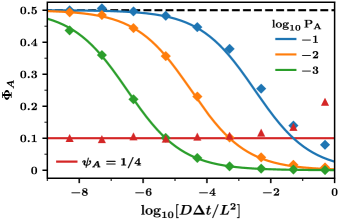
Figure 2: The probability that the Brownian particle reacts with wall $A$, $\Phi_{A}$, for various values of the timestep $\Delta t$. Red triangles correspond to simulations run at $\psi_{A}=1/4$ where the sticking probability at wall $A$, $P_{A}$, varies according to (10). As $\Delta t\to 0$, these simulations approach the analytical result from (13), $\Phi_{A}=1/10$ (red horizontal line). In contrast, the blue, orange, and green diamonds were generated from simulations that used the fixed values of the sticking probability indicated in the upper-right legend. As $\Delta t\to 0$, these data approach $\Phi_{A}=1/2$ (black-dashed line), the infinitely fast reaction limit, following the predictions of (9) and (13) (blue, orange, and green curves). All numerical data points were generated using $10^{4}$ samples. Error bars constructed from Wald confidence intervals are smaller than the symbols [35].

III.3 Previous Studies Treated the Sticking Probability as a Physical Parameter

We now compare our conceptual framework for discrete reactive deposition, which is based on the Damköhler number, with the approach used by previous authors, which is based on the sticking probability. In particular, we focus on off-lattice deposition, where the particles move in continuous space. Many authors instead studied lattice-based systems which we discuss in Sec. LABEL:si:lattice [4, 6].

Prior studies considered the sticking probability $P$ to be a fundamental physical parameter of the system that controlled the surface reaction rate rather than a convergence parameter like $\Delta t$ [8, 36, 9]. This view of the sticking probability appeared to be borne out in simulations where different fixed values of $P$ were found to generate different cluster morphologies [8, 9]. Consequently, Halsey and Leibig proposed that the critical radius for the CTD transition should scale as a power law with $P$ in the limit $P\to 0$ and attempted to use simulations to calculate the associated exponent [8].

Eq. (9) and Fig. 2, however, illustrate that treating the sticking probability as a normal physical parameter has a number of conceptual limitations. In particular, all fixed values of $P$ yield the same infinitely fast reaction dynamics in the limit $\Delta t\to 0$. The reason different $P$ values previously seemed to produce different cluster morphologies in simulations was due to the incomplete timestep convergence [8, 9]. In addition, since for any constant $P$, the morphology always crosses over immediately to fractal growth, examining the behavior of the critical radius in the limit as $P\to 0$ is not physically meaningful.

To resolve these issues, we can recast the simulation results of prior studies into the rate constant-based framework we have introduced here. Since these studies happened to use the same timestep for all of their simulations, the effective rate constant $k$ being simulated, (9), is always directly proportional to the sticking probability $P$ [8, 9]. Consequently, the figures and calculations in these references can be adapted to our framework if the appropriate value of the Damköhler number is substituted for each value of $P$. For example, Halsey and Leibig’s estimate of the power-law scaling exponent of the critical radius in terms of the sticking probability can instead be taken as an estimate for the exponent $\gamma$ in (3), yielding $\gamma=-0.25\pm 0.3$ [8, 37].

There is, however, one caveat with the conversion procedure. After the sticking probability is replaced with the Damköhler number, the simulation results cannot be assumed to be converged with respect to the timestep. That is, the only way to guarantee $\Delta t$ convergence to a finite rate constant is to follow the prescription of (9) and take $\Delta t$ and $P$ to zero at the same time. But previous authors instead always treated $P$ as a fixed quantity [8, 9]. Nevertheless, the values of $\Delta t$ these authors happened to choose are comparable to the value of $\Delta t$ we selected for our simulations in this work based on the rigorous convergence procedure described in Sec. LABEL:si:brownian. Consequently, these studies’ $P$ to $\mathrm{Da}$ converted results are likely free of significant timestep-related artifacts.

III.4 The Reaction-Diffusion Length $D/k$

The ratio of the diffusion constant to the reaction rate constant $D/k$ plays a significant role in the CTD transition. As a reminder, in the continuum model, (1), we have $R_{c}\sim D/k$ directly, and in the discrete model, (3), we have $R_{c}\sim D/k$ in the continuum limit if $\gamma=0$. In this section, we show how the Brownian dynamics algorithm helps to clarify the physical meaning of this length scale, offering a new view of the CTD transition.

The Brownian dynamics algorithm implies that one of the key physical parameters in the simulation is the ratio of the sticking probability and the square root of the timestep. This ratio defines a new microscopic rate constant $\kappa$

$$\kappa=\frac{P}{\sqrt{\Delta t}}=k\sqrt{\frac{\pi}{D}}$$ (14)

that can be used in place of the macroscopic rate constant $k$ [15, 30].

Thinking in terms of $\kappa$ is helpful for understanding the ratio $D/k$. Specifically, since it has units of reciprocal square root of time, $\kappa$ clearly indicates that the timescale for the surface reaction $T$ is

$$T\sim 1/\kappa^{2}\sim D/k^{2}.$$ (15)

The definition of $T$ is not immediately apparent based on the macroscopic view of the system since if we start from the macroscopic rate constant $k$, we find both $a/k$ and $D/k^{2}$ have units of time. Based on (15), we can see that the ratio $D/k$ is the length a particle can diffuse in the characteristic reaction timescale

$$\sqrt{DT}\sim D/k.$$ (16)

Consequently, we call this quantity the “reaction-diffusion length.”

Using the reaction-diffusion length, we can propose a new mechanistic interpretation of the CTD transition. Specifically, $D/k$ scaling of the critical radius implies that dendritic growth initiates when particles can no longer diffuse around the circumference of the cluster within the characteristic reaction timescale. This mechanism helps explain dendrite formation in the continuum model where $R_{c}\sim D/k$. However, critically, it also applies to the discrete model if $\gamma=0$. If instead, $\gamma\neq 0$, the discrete CTD transition must result from some other physical process that the continuum perspective fails to adequately capture. Consequently, determining the value of $\gamma$ is paramount for advancing understanding of dendritic growth and for potentially unifying this understanding across the discrete and continuum scales.

III.5 The Critical Radius $R_{c}$

In this subsection, we define the critical radius quantitatively so that it can be calculated in simulations. The definition we use is posed in terms of the instantaneous fractal dimension of the cluster

$$\mathcal{D}_{F}=\frac{d\log_{10}N}{d\log_{10}(kR_{g}/D)}.$$ (17)

Here, $N$ is the number of particles in the cluster, and $R_{g}$ is the cluster’s radius of gyration. For compact growth, $\mathcal{D}_{F}$ approaches the dimension of the space $d$ after initial transients decay. In contrast, for dendritic growth, $\mathcal{D}_{F}$ plateaus at a characteristic value less than $d$, once again after initial transient behavior. The value of $\mathcal{D}_{F}$ in this dendritic regime has empirically been found to be $1.71$ in 2D and $2.51$ in 3D independent of the value of $\mathrm{Da}$ [6, 38, 8]. As a result of the two plateaus, plots of the fractal dimension versus the log of the cluster radius, such as Fig. 3(a), are roughly sigmoidal.

Based on this behavior, we take the critical radius, $R_{c}$, to be the x-value on the fractal dimension curve with the most negative slope

$$R_{c}=\mathrm{argmin}_{R_{g}}\frac{d\mathcal{D}_{F}}{d\log_{10}(kR_{g}/D)}.$$ (18)

We evaluate (18) using simulation data by first calculating fractal dimension and its derivative with finite difference. We then apply cubic splines to fit the resulting data before taking the $\mathrm{argmin}$.

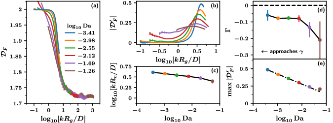
Figure 3: Continuum limit scaling analysis of the compact-to-dendritic transition in two dimensions. All error bars are bootstrapped $95\%$ confidence intervals (CI) and are sometimes smaller than the lines or symbols. See Table LABEL:tab:scaling for further trajectory details. (a) The fractal dimension $\mathcal{D}_{F}$ versus the radius of gyration $R_{g}$ for various values of the Damköhler number, $\mathrm{Da}$. (b) Absolute value of the derivative of the fractal dimension $|\mathcal{D}_{F}^{\prime}|$. The peaks define the critical radius at each value of $\mathrm{Da}$, see (18). (c) The critical radius $R_{c}$ as a function of Damköhler number. (d) The derivative of panel (c), $\Gamma$, which provides an estimate for the scaling exponent $\gamma$ in (3) as $\mathrm{Da}\to 0$. The leftmost (blue) point has a value of $-0.06$ with a $95\%$CI of $[-0.03,-0.09]$. At the top of the panel, the black dashed line represents the hypothesis that $\gamma=0$. (e) The maximum value of $|\mathcal{D}_{F}^{\prime}|$ (or equivalently $|\mathcal{D}_{F}^{\prime}|$ evaluated at critical radius) versus the Damköhler number. A linear fit to the three points with the lowest $\mathrm{Da}$ values (dash-dot black line) has a slope of $-0.15$ with a $95\%$CI of $[-0.16,-0.14]$.

III.6 Calculating the Critical Radius Scaling Exponent $\gamma$

We now describe how we calculate the critical radius scaling exponent $\gamma$ from simulation data and contrast our approach with the one taken by previous authors. We compute $\gamma$ by finding the slope of a log-log plot of the critical radius versus the Damköhler number in the limit as the latter goes to zero. While conceptually straightforward, this method requires evaluating the critical radius at very small values of $\mathrm{Da}$. This procedure is computationally challenging for two reasons. First, as $\mathrm{Da}$ gets smaller, an increasing number of particles are needed to observe the fractal transition, especially in 3D. $N_{c}$, the number of particles in a $d$ dimensional critical cluster, scales as

$$N_{c}\sim(R_{c}/a)^{d}\sim\mathrm{Da}^{d(\gamma-1)},$$ (19)

and based on analyses so far, it is clear $\gamma<1$ [6, 8]. Second, since $\mathrm{Da}$ is proportional to the sticking probability in (10), the smaller its value, the longer it takes each particle to deposit in terms of computational steps.

As described in Sec. LABEL:si:brownian, we used a parallel Brownian dynamics algorithm to help partially alleviate these two problems. However, calculating $\gamma$ still required substantial computational effort because the goal was always to probe deeper into the continuum limit, $\mathrm{Da}\to 0$. In the end, we used large-scale simulations to examine $\mathrm{Da}$ values where the critical clusters in 2D and 3D contained several hundred million particles, orders of magnitude more particles than the largest reactive deposition clusters generated previously [6, 8].

Authors of prior studies calculated $\gamma$ using an alternative strategy. Rather than computing the critical radius directly, these authors instead determined $\gamma$ by exploiting data collapse [6, 8, 39]. As an example of this approach, consider the relationship between the fractal dimension and the cluster radius in nondimensional form

$$\mathcal{D}_{F}=f(\frac{kR_{g}}{D},\mathrm{Da}).$$ (20)

Taking the continuum limit and using the fact that the cluster starts off compact, $\mathcal{D}_{F}=2$, yields

$$\mathcal{D}_{F}=g(\frac{kR_{g}}{\mathrm{Da}^{\gamma}D})$$ (21)

where the factor $\mathrm{Da}^{\gamma}$ is associated with the critical radius [18]. As a result, it is possible to evaluate $\gamma$ by probing the collapse of the fractal dimension data in the low $\mathrm{Da}$ limit.

However, such collapse-based methods have several limitations. To begin with, quantitatively characterizing the extent of a collapse is not straightforward. Previous authors instead estimated $\gamma$ by judging each potential collapse by eye [6, 8]. In addition, equations such as (21) only apply if the Damköhler number is small enough. Consequently, it is necessary to leave out the highest $\mathrm{Da}$ value, then the next highest $\mathrm{Da}$ value, and so on, to assess convergence. Previous authors, however, did not investigate convergence in a systematic matter [6, 8]. Finally, checking for a collapse is susceptible to bias if only partial data is available. For example, at certain values of $\mathrm{Da}$, we often cannot generate large enough clusters to see the full fractal plateau. Running a collapse calculation on such data would artificially add weight to the initial compact piece of the curve that we can successfully compute.

In contrast, directly measuring the critical radius provides a simple way to calculate $\gamma$ and evaluate convergence. All that is necessary is to examine a log-log plot of $R_{c}$ versus $\mathrm{Da}$. Further, direct measurement also avoids introducing any bias due to partial data.

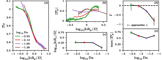
Figure 4: Continuum limit scaling of the compact-to-dendritic transition in three dimensions. Panel axis labels are the same as in Fig. 3, but note the difference in scale between panel (d) and Fig. 3(d). The repeated caption is provide for convenience. See Table LABEL:tab:3d_scaling for further trajectory details. (a) Fractal dimension $\mathcal{D}_{F}$ as a function of the radius of gyration $R_{g}$ for different Damköhler numbers, $\mathrm{Da}$. (b) The absolute value of the derivative of panel (a), $|\mathcal{D}_{F}^{\prime}|$. (c) The critical radius $R_{c}$ versus $\mathrm{Da}$. (d) Derivative of the log of the critical radius with respect to the log of the Damköhler number, $\Gamma$. The black dashed line corresponds to the $\gamma=0$ hypothesis. (e) Height of the peak in panel (b), $\max|\mathcal{D}_{F}^{\prime}|$, versus the Damköhler number.

IV Results and Discussion

In this section, we present the results of our two and three-dimensional Brownian dynamics simulations and evaluate whether these results are consistent with the $\gamma=0$ hypothesis. We also explore the sharpening of the CTD transition in the continuum limit, a feature of the system that resembles the finite-size scaling of an equilibrium phase transition.

Simulation results for two-dimensional deposition are shown in Fig. 3. Panel (a) exhibits the characteristic sigmoidal shape of the fractal dimension as a function of the cluster radius. At smaller values of the Damköhler number, the fractal transition occurs when the cluster has very few particles. For this reason, the plateau at $\mathcal{D}_{F}=2$ due to compact growth is not yet fully visible. The lack of this compact plateau makes calculating the critical radius impossible at $\log_{10}\mathrm{Da}$ values larger than $-1.26$. Panel (a) also provides further evidence that the fractal dimension of 2D dendritic growth is approximately $1.71$ independent of the value of $\mathrm{Da}$ [6, 8].

From Fig. 3(a), we can calculate the critical radius, (18), and evaluate its behavior in the continuum limit. Fig. 3(b) shows the magnitude of the derivative of the fractal dimension. The peaks on this panel define the critical radius $R_{c}$ for each $\mathrm{Da}$. Plotting these $R_{c}$ values directly in Fig. 3(c) shows that the critical radius increases as the Damköhler number gets smaller. To find the exponent $\gamma$, in panel (d) we compute the derivative $\Gamma=\frac{d\log_{10}[kR_{c}/D]}{d\log_{10}\mathrm{Da}}$ which converges to $\gamma$ in the limit $\mathrm{Da}\to 0$. We find that this derivative gets closer to zero as $\mathrm{Da}$ gets smaller. Further, taking the leftmost point on the curve (blue) to approximate $\gamma$ yields an estimate of $-0.06$ with a $95\%$CI of $[-0.09,-0.03]$.

The confidence interval for $\gamma$ must be interpreted carefully in relation to the $\gamma=0$ hypothesis. In particular, this interval does not include zero. The remaining discrepancy can be explained by the magnitude of the Damköhler number. That is, for smaller values of $\mathrm{Da}$, $\Gamma$ might follow the trend in Fig. 3(d) and move closer to zero. But this trend is not robust. The bottom of the confidence interval for the blue point, $-0.09$, may instead indicate that the final part of the upwards drift in the data is a numerical artifact covering an underlying plateau at a value of around $-0.1$. Such a plateau would be consistent with the position of the preceding orange, green, and red points.

In spite of this concern about the trend in $\Gamma$, we can draw two conclusions from the results of the 2D simulations. First, previous studies reported that $\gamma\approx-0.2$, but this value does not fit our data [6, 8]. Based on panel (d), it is clear that $\gamma\geq-0.1$, a significant upward revision. Second, while it is not possible to distinguish between a plateau at around $\gamma=-0.1$ and a continued trend towards $\gamma=0$, the latter is still entirely consistent with the simulation results. Consequently, the data offers the first substantial numerical support for the hypothesis that $\gamma=0$.

We now turn toward characterizing the critical radius of the CTD transition in 3D. The results of our 3D simulations are presented in Fig. 4 using the same format as the 2D results. In panel (c), as $\mathrm{Da}$ tends towards zero, $R_{c}$ exhibits an immediate plateau at a value of around $3D/k$. Again using the leftmost point of panel (d), we find that $\gamma=0.02$ with a $95\%$CI of $[-0.27,0.12]$. This confidence interval is very broad due to the limited number of trajectories generated at $\log_{10}\mathrm{Da}=-2.55$. To increase the precision, we can instead estimate $\gamma$ using the second-to-last point from the left (red), which has a value of $-0.01$ with a $95\%$CI of $[-0.11,0.02]$. However, by using a larger value of the Damköhler number, we may sacrifice some accuracy with respect to the $\mathrm{Da}\to 0$ limit.

Using the 3D data to evaluate the $\gamma=0$ hypothesis presents its own set of challenges because simulations in this dimension are more expensive than in 2D. To begin with, we could not observe the CTD transition at as wide a range of Damköhler numbers, and as a result, the convergence to the $\mathrm{Da}\to 0$ limit is not as robust. For example, unlike in 2D, the plateau that corresponds to the compact growth regime $\mathcal{D}_{F}=3$ is not fully developed in Fig. 4(a) even for the smallest value of $\log_{10}\mathrm{Da}=-2.55$ (green curve). In addition, since we generated fewer trajectories overall, the error bars in Fig. 4 are wider than in Fig. 3. For this reason, although the flattening trend in the 3D data is clear, it is not possible to rule out plateau at a $\gamma$ value between zero and $-0.1$.

Despite these limitations, the estimate for $\gamma$ in 3D is consistent with the $2D$ estimate, $95\%$CI $[-0.09,-0.03]$. Further, taken together, the 2D and 3D data sets offer significant evidence for the $\gamma=0$ hypothesis. Both $\gamma$ confidence intervals are close to zero, and the remaining differences can be plausibly explained by Damköhler number and statistical convergence effects.

These findings clarify the behavior of CTD transition in two ways. First, they suggest that the continuum limit of the discrete model, $\mathrm{Da}\to 0$, is well-defined. Once the particles become small enough, the critical radius rescaled by $D/k$ converges to a constant. Second, our results help unify the discrete and continuum models by showing that they exhibit the same dendrite formation mechanism. In both cases, the dendritic instability develops when the cluster circumference exceeds the reaction-diffusion length $D/k$. The ability of the continuum model to reproduce the microscopic physics of the discrete model is important because it validates the continuum approach to studying dendritic deposition more generally. In particular, this agreement provides a stronger microscopic foundation for a number of research efforts that have used continuum methods to examine electrodeposition applications including dendrite suppression strategies in lithium metal batteries [21, 22, 23, 24, 25, 26, 27, 28]

One last feature of the CTD transition that warrants discussion is its sharpness. Fig. 3(b) shows that, in 2D, the height of the peak in the fractal dimension derivative, $|\mathcal{D}_{F}^{\prime}|$, appears to diverge in the limit as $\mathrm{Da}\to 0$. This behavior is notable because as $\mathrm{Da}$ gets smaller, the number of particles in the critical cluster, $N_{c}$ in (19), goes to infinity. The sharpening of the CTD transition is thus reminiscent of the finite-size scaling of an equilibrium phase transition [40].

This connection motivates us to analyze the transition by following the standard equilibrium protocol. Specifically, we examine the scale of the divergence and the associated prefactor [40]. Fig. 3(e) shows the height of the peak in the derivative, $\max|\mathcal{D}_{F}^{\prime}|$, as a function of the Damköhler number. The line of best fit suggests that this quantity diverges logarithmically with a prefactor of $-0.15$ ($95\%$CI of $[-0.16,-0.14]$). However, since the range of values in the figure is relatively small, it is not possible to distinguish between a logarithmic and a power-law divergence. The latter case leads to a best-fit exponent with the same value as the logarithmic prefactor, $-0.15$ with a $95\%$CI of $[-0.16,-0.14]$. Figs. 4(b) and (e) show that the CTD transition also becomes increasingly sharp in 3D, though we do not yet have enough points to evaluate the prefactor in this dimension.

Beyond a numerical characterization of the divergence of $|\mathcal{D}_{F}^{\prime}|$, many aspects of the finite-size scaling of the CTD transition remain unclear. For example, how does this divergence emerge from the microscopic dynamics? And how does the behavior of the transition relate to finite-size scaling in equilibrium? We hope to pursue these questions in the future.

V Conclusion

In this work, we examined the CTD transition in reactive deposition to clarify how the dendritic branch thickness depends on the deposition parameters. Specifically, we compared the behavior of the CTD transition in an analytically tractable continuum model and a particle-based (discrete) model. In contrast with previous studies, we found that Brownian dynamics simulations of the discrete model in the continuum limit are consistent with the behavior of the continuum model. That is, the critical radius is proportional to the ratio of the diffusion constant to the reaction rate constant. This behavior implies that these models share the same mechanism for dendritic growth. In each case, dendrites emerge when the circumference of the cluster becomes comparable to the reaction-diffusion length. More broadly, our findings suggest that continuum formulations of reactive deposition, which are widely used to study lithium metal batteries and other types of electrodeposition, are able to accurately reproduce the microscopic features of dendrite formation [21, 22, 23, 24, 25, 26, 27, 28].

Future investigations will test whether the CTD transition displays the same phenomenology in real, as opposed to idealized, systems with the aim of managing dendritic deposition in applications like batteries. In experiments, the continuum limit could be accessed by making the reaction rate slower rather than changing the radius of the microscopic particles. This procedure would be particularly practical in electrochemistry since the applied voltage directly controls the surface reaction kinetics [41]. However, we also expect reaction-diffusion length scaling to apply to many other systems, including those that feature the deposition of colloids or misfolded proteins.

Finally, it remains to be seen how the CTD transition interacts with more complicated deposition geometries. Here, we examined a cluster that grows outwards in all directions. This configuration has been the focus of previous computational and theoretical efforts due to its simplicity [31]. However, another possible choice is to grow the cluster upwards starting from a reactive surface at the bottom of a box, a geometry that more closely resembles a standard electrodeposition experiment [42, 9]. Intriguingly, the confinement provided by the box walls has been shown to suppress dendritic growth in experiments and continuum scale models [25, 26, 27]. We plan to characterize the CTD transition in this type of deposition in a future publication.

VI Acknowledgments

We thank Steve Whitelam, Tomislav Begušić, and Emiliano Deustua for providing comments on the manuscript. DJ acknowledges support from the Department of Energy Computational Science Graduate Fellowship, under Contract No. DE-FG02–97ER25308. This work was supported by a grant from NIGMS, National Institutes of Health, (R01GM125063) to TFM.

References

- Lin et al. [1989] M. Y. Lin, H. M. Lindsay, D. A. Weitz, R. C. Ball, R. Klein, and P. Meakin, Nature 339, 360 (1989).
- Foderà et al. [2013] V. Foderà, A. Zaccone, M. Lattuada, and A. M. Donald, Physical Review Letters 111, 108105 (2013).
- Kahanda et al. [1992] G. L. M. K. S. Kahanda, X.-q. Zou, R. Farrell, and P.-z. Wong, Physical Review Letters 68, 3741 (1992).
- Witten and Sander [1983] T. A. Witten and L. M. Sander, Physical Review B 27, 5686 (1983).
- Meakin [1983] P. Meakin, Physical Review A 27, 1495 (1983).
- Meakin [1988] P. Meakin, Annual Review of Physical Chemistry 39, 237 (1988).
- Nagatani [1989] T. Nagatani, Physical Review A 40, 7286 (1989).
- Halsey and Leibig [1990] T. C. Halsey and M. Leibig, The Journal of Chemical Physics 92, 3756 (1990).
- Mayers et al. [2012] M. Z. Mayers, J. W. Kaminski, and T. F. Miller, The Journal of Physical Chemistry C 116, 26214 (2012).
- Mullins and Sekerka [1963] W. W. Mullins and R. F. Sekerka, Journal of Applied Physics 34, 323 (1963).
- Liu et al. [2018] K. Liu, Y. Liu, D. Lin, A. Pei, and Y. Cui, Science Advances 4, eaas9820 (2018).
- Lin et al. [2017] D. Lin, Y. Liu, and Y. Cui, Nature Nanotechnology 12, 194 (2017).
- Hwang et al. [2017] J.-Y. Hwang, S.-T. Myung, and Y.-K. Sun, Chemical Society Reviews 46, 3529 (2017).
- Note [1] Meakin suggested that the initial phase of compact deposition is linked to Eden growth, reasoning that, when the cluster is small enough, incoming particles equilibrate with its surface and become equally likely to deposit everywhere [43, 31].
- Erban and Chapman [2007] R. Erban and S. J. Chapman, Physical Biology 4, 16 (2007).
- Note [2] See also Sec. LABEL:si:linear.
- Witten and Sander [1981] T. A. Witten and L. M. Sander, Physical Review Letters 47, 1400 (1981).
- Barenblatt [1996] G. I. Barenblatt, Scaling, Self-similarity, and Intermediate Asymptotics: Dimensional Analysis and Intermediate Asymptotics (Cambridge University Press, 1996) pp. 1–386.
- Note [3] Choosing to nondimensionalize the critical radius by the particle radius provides a different, though equivalent, scaling relationship [4, 6, 8].
- Note [4] See also Sections III and LABEL:si:lattice.
- Aogaki [1982] R. Aogaki, Journal of The Electrochemical Society 129, 2442 (1982).
- Sundström and Bark [1995] L.-G. Sundström and F. H. Bark, Electrochimica Acta 40, 599 (1995).
- Monroe and Newman [2004] C. Monroe and J. Newman, Journal of The Electrochemical Society 151, A880 (2004).
- Monroe and Newman [2005] C. Monroe and J. Newman, Journal of The Electrochemical Society 152, A396 (2005).
- Tikekar et al. [2014] M. D. Tikekar, L. A. Archer, and D. L. Koch, Journal of The Electrochemical Society 161, A847 (2014).
- Liu et al. [2016] W. Liu, D. Lin, A. Pei, and Y. Cui, Journal of the American Chemical Society 138, 15443 (2016).
- Tu et al. [2017] Z. Tu, M. J. Zachman, S. Choudhury, S. Wei, L. Ma, Y. Yang, L. F. Kourkoutis, and L. A. Archer, Advanced Energy Materials 7, 1602367 (2017).
- Choudhury et al. [2018] S. Choudhury, D. Vu, A. Warren, M. D. Tikekar, Z. Tu, and L. A. Archer, Proceedings of the National Academy of Sciences 115, 6620 (2018).
- Hastings and Levitov [1998] M. Hastings and L. Levitov, Physica D: Nonlinear Phenomena 116, 244 (1998).
- Singer et al. [2008] A. Singer, Z. Schuss, A. Osipov, and D. Holcman, SIAM Journal on Applied Mathematics 68, 844 (2008).
- Meakin [1998] P. Meakin, Fractals, Scaling and Growth Far from Equilibrium, Cambridge Nonlinear Science Series No. 5 (Cambridge University Press, Cambridge [England] ; New York, 1998).
- Niemeyer et al. [1984] L. Niemeyer, L. Pietronero, and H. J. Wiesmann, Physical Review Letters 52, 1033 (1984).
- Pietronero and Wiesmann [1984] L. Pietronero and H. J. Wiesmann, Journal of Statistical Physics 36, 909 (1984).
- Allen and Tildesley [2017] M. P. Allen and D. J. Tildesley, Computer Simulation of Liquids, second edition ed. (Oxford University Press, Oxford, United Kingdom, 2017).
- Agresti and Coull [1998] A. Agresti and B. A. Coull, The American Statistician 52, 119 (1998).
- Nagatani and Stanley [1990] T. Nagatani and H. E. Stanley, Physical Review A 41, 3263 (1990).
- Note [5] Ref. \rev@citealpmeakinFractalsScalingGrowth1998 states that Halsey and Leibig’s result in Ref. \rev@citealphalseyElectrodepositionDiffusionLimited1990 is consistent with instead of . However, we believe this is in error based on Eq. in the original reference.
- Tolman and Meakin [1989] S. Tolman and P. Meakin, Physical Review A 40, 428 (1989).
- Note [6] Meakin in Ref. \rev@citealpmeakinModelsColloidalAggregation1988 actually estimated the equivalent lattice-based scaling exponent instead of , see Sec. LABEL:si:lattice. However, the same data collapse method was used for this calculation.
- Newman [1999] M. E. J. Newman, Monte Carlo Methods in Statistical Physics (Clarendon Press ; Oxford University Press, Oxford : New York, 1999).
- Bard and Faulkner [2001] A. J. Bard and L. R. Faulkner, Electrochemical Methods: Fundamentals and Applications, 2nd ed. (Wiley, New York, 2001).
- Somfai et al. [2003] E. Somfai, R. C. Ball, J. P. DeVita, and L. M. Sander, Physical Review E 68, 020401 (2003).
- Meakin [1986] P. Meakin, in On Growth and Form: Fractal and Non-Fractal Patterns in Physics, NATO ASI Series, edited by H. E. Stanley and N. Ostrowsky (Springer Netherlands, Dordrecht, 1986) pp. 111–135.