Perfect: Prompt-free and Efficient Few-shot Learning with Language Models

Abstract

Current methods for few-shot fine-tuning of pretrained masked language models (PLMs) require carefully engineered prompts and verbalizers for each new task to convert examples into a cloze-format that the PLM can score. In this work, we propose Perfect, a simple and efficient method for few-shot fine-tuning of PLMs without relying on any such handcrafting, which is highly effective given as few as 32 data points. Perfect makes two key design choices: First, we show that manually engineered task prompts can be replaced with task-specific adapters that enable sample-efficient fine-tuning and reduce memory and storage costs by roughly factors of 5 and 100, respectively. Second, instead of using handcrafted verbalizers, we learn new multi-token label embeddings during fine-tuning, which are not tied to the model vocabulary and which allow us to avoid complex auto-regressive decoding. These embeddings are not only learnable from limited data but also enable nearly 100x faster training and inference. Experiments on a wide range of few shot NLP tasks demonstrate that Perfect, while being simple and efficient, also outperforms existing state-of-the-art few-shot learning methods. Our code is publicly available at https://github.com/facebookresearch/perfect.git.

1 Introduction

Recent methods for few-shot language model tuning obtain impressive performance but require careful engineering of prompts and verbalizers to convert inputs to a cloze-format (Taylor, 1953) that can be scored with pre-trained language models (PLMs) (Radford et al., 2018, ; Brown et al., 2020; Schick and Schütze, 2021a, b). For example, as Figure 1 shows, a sentiment classifier can be designed by inserting the input text $\bm{x}$ in a prompt template “$\bm{x}$ It was [MASK]” where verbalizers (e.g., ‘great’ and ‘terrible’) are substituted for the [MASK] to score target task labels (‘positive’ or ‘negative’). In this paper, we show that such engineering is not needed for few-shot learning and instead can be replaced with simple methods for data-efficient fine-tuning with as few as 32 end-task examples.

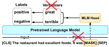
Figure 1: Existing few-shot fine-tuning methods require manual engineering to reduce new tasks to masked language modeling. Perfect does not rely on any handcrafting, removing both patterns and verbalizers (see Figure 3).

More specifically, we propose Perfect, a Prompt-free and Efficient paRadigm for FEw-shot Cloze-based fine-Tuning. To remove handcrafted patterns, Perfect uses task-specific adapter layers Houlsby et al. (2019); Pfeiffer et al. (2020) (§3.1). Freezing the underlying PLM with millions or billions of parameters (Liu et al., 2019; Raffel et al., 2020), and only tuning adapters with very few new parameters saves on memory and storage costs (§4.2), while allowing very sample-efficient tuning (§4). It also stabilizes the training by increasing the worst-case performance and decreasing variance across the choice of examples in the few shot training sets (§4.3).

To remove handcrafted verbalizers (with variable token lengths), we introduce a new multi-token fixed-length classifier scheme that learns task label embeddings which are independent from the language model vocabulary during fine-tuning (§3.2). We show (§4) that this approach is sample efficient and outperforms carefully engineered verbalizers from random initialization (§4). It also allows us to avoid previously used expensive auto-regressive decoding schemes (Schick and Schütze, 2021b), by leveraging prototypical networks (Snell et al., 2017) over multiple tokens. Overall, these changes enable up to 100x faster learning and inference (§4.2).

Perfect has several advantages: It avoids engineering patterns and verbalizers for each new task, which can be cumbersome. Recent work has shown that even some intentionally irrelevant or misleading prompts can perform as well as more interpretable ones Webson and Pavlick (2021). Unlike the zero-shot or extreme few-shot case, where prompting might be essential, we argue in this paper that all you need is tens of training examples to avoid these challenges by adopting Perfect or a similar data-efficient learning method. Experiments on a wide variety of NLP tasks demonstrate that Perfect outperforms state-of-the-art prompt-based methods while being significantly more efficient in inference and training time, storage, and memory usage (§4.2). To the best of our knowledge, we are the first to propose a few-shot learning method using the MLM objective in PLMs that provide state-of-the-art results while removing all per-task manual engineering.

2 Background

Problem formulation:

We consider a general problem of fine-tuning language models in a few-shot setting, on a small training set with $K$ unique classes and $N$ examples per class, such that the total number of examples is $|\mathcal{D}|=N\times K$. Let $\mathcal{D}=\cup_{k=1}^{K}\mathcal{D}_{k}$ be the given training set, where $\mathcal{D}_{k}=\{(\bm{x^{i}_{k}},y^{i}_{k})\}_{i=1}^{N}$ shows the set of examples labeled with class $k$ and $y^{i}_{k}\in\mathcal{Y}$ is the corresponding label, where $|\mathcal{Y}|=K$. We additionally assume access to a development set with the same size as the training data. Note that larger validation sets can grant a substantial advantage (Perez et al., 2021), and thus it is important to use a limited validation size to be in line with the goal of few-shot learning. Unless specified otherwise, in this work, we use 16 training examples ($N=16$) and a validation set with 16 examples, for a total of 32-shot learning.

2.1 Adapters

Recent work has shown that fine-tuning all parameters of PLMs with a large number of parameters in low-resource datasets can lead to a sub-optimal solution (Peters et al., 2019; Dodge et al., 2020). As shown in Figure 2, Rebuffi et al. (2018) and Houlsby et al. (2019) suggest an efficient alternative, by inserting small task-specific modules called adapters within layers of a PLMs. They then only train the newly added adapters and layer normalization, while fixing the remaining parameters of a PLM.

Each layer of a transformer model is composed of two primary modules: a) an attention block, and b) a feed-forward block, where both modules are followed by a skip connection. As depicted in Figure 2, adapters are normally inserted after each of these blocks before the skip connection.

Adapters are bottleneck architectures. By keeping input and output dimensions the same, they introduce no additional architectural changes. Each adapter, $A(.)\in\mathbb{R}^{H}$, consists of a down-projection, $D(.)\in\mathbb{R}^{H\times B}$, a non-linearity, such as GeLU (Hendrycks and Gimpel, 2016), and an up-projection $U(.)\in\mathbb{R}^{B\times H}$, where $H$ is the dimension of input hidden states $\bm{x}$, and $B$ is the bottleneck size. Formally defined as:

$$A(\bm{x})=U(\text{GeLU}(D(\bm{x})))+\bm{x},$$ (1)

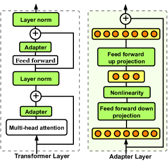
Figure 2: Left: Adapter integration in a PLM. Right: An adapter architecture. Adapters are usually inserted after the feed-forward and self-attention modules. During training, we only optimize the green components

2.2 Prompt-based Fine-tuning

Standard Fine-tuning:

In standard fine-tuning with PLMs (Devlin et al., 2019), first a special [CLS] token is appended to the input $\bm{x}$, and then the PLM maps it to a sequence of hidden representations $\bm{h}=(\bm{h_{1}},\dots,\bm{h_{S}})$ with $\bm{h_{i}}\in\mathbb{R}^{H}$, where $H$ is the hidden dimension, and $S$ is the maximum sequence length. Then, a classifier, $\textit{softmax}(\bm{W^{T}}\bm{h}_{\text{[CLS]}})$, using the embedding of the classification token ($\bm{h}_{\text{[CLS]}}$), is trained end-to-end for each downstream task. The main drawback of this approach is the discrepancy between the pre-training and fine-tuning phases since PLMs have been trained to predict mask tokens in a masked language modeling task (Devlin et al., 2019).

Prompt-based tuning:

To address this discrepancy, prompt-based fine-tuning (Schick and Schütze, 2021a, b; Gao et al., 2021) formulates tasks in a cloze-format (Taylor, 1953). This way, the model can predict targets with a masked language modeling (MLM) objective. For example, as shown in Figure 1, for a sentiment classification task, inputs are converted to:

$$\bm{x}_{\text{prompt}}~{}=~{}\text{[CLS]}~{}\bm{x}~{}.~{}\underbrace{\text{It was}}_{\text{pattern}}~{}\text{[MASK]}~{}.~{}\text{[SEP]}$$

Then, the PLM determines which verbalizer (e.g., ‘great’ and ‘terrible’) is the most likely substitute for the mask in the $\bm{x}_{\text{prompt}}$. This subsequently determines the score of targets (‘positive’ or ‘negative’). In detail:

Training strategy:

Let $\mathcal{M}:\mathcal{Y}\to\mathcal{V}$ be a mapping from target labels to individual words in a PLM’s vocabulary. We refer to this mapping as verbalizers. Then the input is converted to $\bm{x}_{\text{prompt}}=\mathcal{T}(\bm{x})$ by appending a pattern and a mask token to $\bm{x}$ so that it has the format of a masked language modeling input. Then, the classification task is converted to a MLM objective (Tam et al., 2021; Schick and Schütze, 2021a), and the PLM computes the probability of the label $y$ as:

$$p(y|\bm{x}) =p(\text{[MASK]}=\mathcal{M}(y)|\bm{x}_{\text{prompt}})$$

$$=\frac{\exp(\bm{W}_{\mathcal{M}(y)}^{T}\bm{h}_{\text{[MASK]}})}{\sum_{v^{\prime}\in\mathcal{V}}\exp(\bm{W}^{T}_{v^{\prime}}\bm{h}_{\text{[MASK]}})},$$ (2)

where $\bm{h}_{\text{[MASK]}}$ is the last hidden representation of the mask, and $\bm{W}_{v}$ shows the output embedding of the PLM for each verbalizer $v\in\mathcal{V}$. For many tasks, verbalizers have multiple tokens. Schick and Schütze (2021b) extended (2) to multiple mask tokens by adding the maximum number of mask tokens $M$ needed to express the outputs (verbalizers) for a task. In that case, Schick and Schütze (2021b) computes the probability of each class as the summation of the log probabilities of each token in the corresponding verbalizer, and then they add a hinge loss to ensure a margin between the correct verbalizer and the incorrect ones.

Inference strategy:

During inference, the model needs to select which verbalizer to use in the given context. Schick and Schütze (2021b) predicts the verbalizer tokens in an autoregressive fashion. They first trim the number of mask tokens from $M$ to each candidate verbalizer’s token length and compute the probability of each mask token. They then choose the predicted token with the highest probability and replace the corresponding mask token. Conditioning on this new token, the probabilities of the remaining mask positions are recomputed. They repeat this autoregressive decoding until they fill all mask positions. This inference strategy is very slow, as the number of forward passes increases with the number of classes and the number of verbalizer’s tokens.

This formulation obtained impressive few-shot performance with PLMs. However, the success of this approach heavily relies on engineering handcrafted patterns and verbalizers. Coming up with suitable verbalizers and patterns can be difficult (Mishra et al., 2022b, a). Additionally, the performance is sensitive to the wording of patterns (Zhao et al., 2021; Perez et al., 2021; Schick and Schütze, 2021a; Jiang et al., 2020) or to the chosen verbalizers (Webson and Pavlick, 2021).

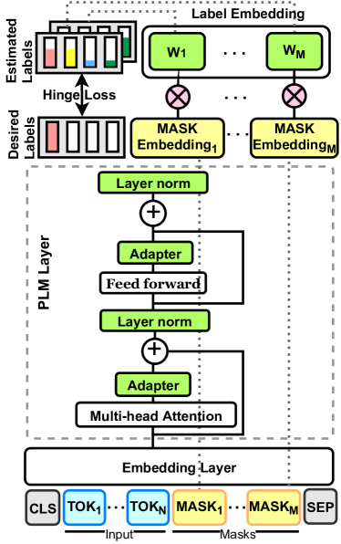
Figure 3: We remove handcrafted patterns and verbalizers. We replace patterns using task-specific adapters and design label embeddings for the classes. We only train the green blocks (the label embeddings, adapters, and layer norms).

In addition, handcrafted verbalizers cause problems for efficient training: a) they require updating the PLM embedding layer, causing large memory overhead; b) fine-tuning PLMs also requires a very small learning rate (usually $10^{-5}$), which slows down tuning the parameters of the verbalizers; c) modeling verbalizers as one of the tokens of the PLM vocabulary (perhaps unintentionally) impacts the input representation during tuning; d) verbalizers have variable token lengths, complicating the implementation in a vectorized format, thereby making it challenging to efficiently fine-tune PLMs.

3 Method

We propose Perfect, a verbalizer and pattern free few-shot learning method. We design Perfect to be close to the pre-training phase, similar to the PET family of models (Schick and Schütze, 2021b; Gao et al., 2021), while replacing handcrafted patterns and verbalizers with new components that are designed to describe the task and learn the labels. As shown in Figure 3, we first convert each input $\bm{x}_{\text{input}}$ to its masked language modeling (MLM) input containing $M$ mask tokens [MASK] with no added patterns, denoted as $\bm{x}_{\text{masked}}=\mathcal{T^{{}^{\prime}}}(\bm{x}_{\text{input}})$. Perfect then trains a classifier per-token and optimizes the average multi-class hinge loss over each mask position.

Three main components play a role in the success of Perfect: a) a pattern-free task description, where we use task-specific adapters to efficiently tell the model about the given task, replacing previously manually engineered patterns (§3.1), b) multi-token label-embedding as an efficient mechanism to learn the label representations, removing manually designed verbalizers (§3.2). c) an efficient inference strategy building on top of the idea of prototypical networks (Snell et al., 2017) (§3.4), which replaces prior iterative autoregressive decoding methods (Schick and Schütze, 2021b).

As shown in Figure 3, we fix the underlying PLM model and only optimize the new parameters that we add (green boxes). This includes the task-specific adapters to adapt the representations for a given task and the multi-token label representations. We detail each of these components below.

3.1 Pattern-Free Task Description

We use task-specific adapter layers to provide the model with learned, implicit task descriptions. Adapters additionally bring multiple other benefits: a) fine-tuning all weights of PLMs with millions or billions of parameters is sample-inefficient, and can be unstable in low-resource settings (Dodge et al., 2020); adapters allow sample-efficient fine-tuning, by keeping the underlying PLM fixed, b) adapters reduce the storage and memory footprints (§4.2), c) they also increase stability and performance (§4), making them an excellent choice for few-shot fine-tuning. To our knowledge, this is the first approach for using task-specific adapters to effectively and efficiently remove patterns in few-shot learning. Experimental results in §4 show its effectiveness compared to handcrafted patterns and soft prompts (Li and Liang, 2021; Lester et al., 2021).

3.2 Multi-Token Label Embeddings

We freeze the weights of the PLM’s embedding layer and introduce a separate label embedding $\bm{L}\in\mathbb{R}^{K\times M\times H}$, which is a multi-token label representation where $M$ is the number of tokens representing each label, $K$ indicates the number of classes, $H$ is the input hidden dimension. Using a fixed number of tokens $M$ for each label, versus variable-token length verbalizers used in prior work (Schick and Schütze, 2021a, b) substantially simplifies the implementation and accelerates the training (§4.2).

3.3 Training Perfect

As shown in Figure 3, we optimize label embeddings so that the PLM predicts the correct label, and optimize adapters to adapt the PLM for the given task. For label embeddings, Perfect trains a classifier per token and optimizes the average multi-class hinge loss over all mask positions. Given $\bm{x}_{\text{masked}}$, let $\bm{h}_{\textsc{[MASK]}_{i}}$ be the embedding of its $i$-th mask token from the last layer of the PLM encoder. Additionally, let $f(.):\mathbb{R}^{H}\to\mathbb{R}^{K}$ be a per-token classifier that computes the predictions by multiplying the mask token embedding with its corresponding label embedding. Formally defined as:

$$\bm{t_{i}}=f(\bm{h}_{\textsc{[MASK]}_{i}})=\bm{L_{i}}^{T}\bm{h}_{\textsc{[MASK]}_{i}},$$

where $\bm{L_{i}}\in\mathbb{R}^{K\times H}$ shows the label embedding for the $i$-th mask position. Then, for each mask position, we optimize a multi-class hinge loss between their scores $\bm{t_{i}}$ and labels. Formally defined as:

$$\mathcal{L}(\bm{x},y,i)=\frac{\sum_{k=1,k\neq y}^{K}\max(0,m-\bm{t_{iy}}+\bm{t_{ik}})}{K},$$

where $\bm{t_{ik}}$ shows the $k$-th element of $\bm{t_{i}}$, representing the score corresponding to class $k$, and $m$ is the margin, which we fix to the default value of $m=1$. Then, the final loss is computed by averaging the loss over all mask tokens and training samples:

$$\mathcal{L}=\frac{1}{M|\mathcal{D}|}\sum_{(\bm{x},y)\in\mathcal{D}}\sum_{i=1}^{M}\mathcal{L}(\bm{x},y,i)$$ (3)

3.4 Inference with Perfect

During evaluation, instead of relying on the prior iterative autoregressive decoding schemes (Schick and Schütze, 2021b), we classify a query point by finding the nearest class prototype to the mask token embeddings:

$$y=\operatornamewithlimits{argmax}_{y\in\mathcal{Y}}\hskip 1.00006pt\max_{i\in\{1,\dots,M\}}\left(\hskip 1.00006pt{\exp^{-d(\bm{h_{i}^{q}},\bm{c_{iy}})}}\right),$$ (4)

where $d$ is squared euclidean distance, $\bm{h_{i}^{q}}$ indicates the embedding of the $i$-th mask position for the query sample $q$, and $\bm{c_{iy}}\in\mathbb{R}^{D}$ is the prototype representation of the $i$-th mask token with class label $y$, i.e., the mean embedding of $i$-th mask position in all training samples with label $y$:

$$\bm{c_{iy}}=\frac{1}{|\mathcal{D}_{y}|}\sum_{b\hskip 0.06996pt\in\mathcal{D}_{y}}\bm{h_{i}^{b}},$$ (5)

where $\bm{h_{i}^{b}}$ shows the embedding of $i$-th mask position for training sample $b$, and $\mathcal{D}_{y}$ is the training instances with class $y$. This strategy closely follows prototypical networks (Snell et al., 2017), but applied across multiple tokens. We choose this form of inference because prototypical networks are known to be sample efficient and robust (Snell et al., 2017), and because it substantially speeds up evaluation compared to prior methods (§4.2).

Method SST-2 CR MR SST-5 Subj TREC Avg Single-Sentence Benchmarks Finetune 81.4/70.0/4.0 80.1/72.9/4.1 77.7/66.8/4.6 39.2/34.3/2.5 90.2/84.1/1.8 87.6/75.8/3.7 76.0/67.3/3.4 PET-Average 89.7/81.0/2.4 88.4/68.8/3.0 85.9/79.0/2.1 45.9/40.3/2.4 88.1/79.6/2.4 85.0/70.6/4.5 80.5/69.9/2.8 PET-Best 89.1/81.0/2.6 88.8/85.8/1.9 86.4/82.0/1.6 46.0/41.2/2.4 88.7/84.6/1.8 85.8/70.6/4.4 80.8/74.2/2.4 Logan IV et al. (2021) 89.8/84.1/1.7 89.9/87.2/1.1 84.9/76.2/3.2 45.7/41.6/2.3 81.8/73.5/4.0 84.7/81.8/1.6 79.5/74.1/2.3 Perfect-rand 90.7/88.2/1.2 90.0/85.5/1.4 86.3/81.4/1.6 42.7/35.1/2.9 89.1/82.8/2.1 90.6/81.6/3.2 81.6/75.8/2.1 Ablation Perfect-init 90.9/87.6/1.5 89.7/87.4/1.2 85.4/75.8/3.3 42.8/35.9/3.5 87.6/81.6/2.8 90.4/86.6/1.8 81.1/75.8/2.4 prompt+mte 70.6/56.0/8.3 71.0/55.8/8.2 66.6/49.6/7.3 32.2/26.5/3.2 82.7/69.6/3.9 79.6/66.8/6.5 67.1/54.0/6.2 bitfit+mte 89.5/81.7/3.0 90.1/87.8/1.0 85.6/80.5/1.9 42.3/36.8/3.3 89.1/82.4/2.4 90.4/85.0/1.4 81.2/75.7/2.2 Method CB RTE QNLI MRPC QQP WiC Avg Sentence-Pair Benchmarks Finetune 72.9/67.9/2.5 56.8/50.2/3.5 62.7/51.4/7.0 70.1/62.7/4.7 65.0/59.8/3.6 52.4/46.1/3.7 63.3/56.4/4.2 PET-Average 86.9/73.2/5.1 60.1/49.5/4.7 66.5/55.7/6.2 62.1/38.2/6.8 63.4/44.7/7.9 51.0/46.1/2.6 65.0/51.2/5.6 PET-Best 90.0/78.6/3.9 62.3/51.3/4.5 70.5/57.9/6.4 63.4/49.3/6.5 70.7/55.2/5.8 51.6/47.2/2.3 68.1/56.6/4.9 Logan IV et al. (2021) 91.0/87.5/2.7 64.4/58.5/3.9 71.2/66.5/2.6 63.9/53.7/5.3 70.4/62.7/3.4 52.4/48.4/1.8 68.9/62.9/3.3 Perfect-rand 90.3/83.9/3.5 60.4/53.1/4.7 74.1/60.3/4.6 67.8/54.7/5.7 71.2/64.2/3.5 53.8/47.0/3.0 69.6/60.5/4.2 Ablation Perfect-init 87.9/75.0/4.9 60.7/52.7/4.5 72.8/56.7/6.8 65.9/56.6/6.0 71.1/65.6/3.5 51.7/46.6/2.8 68.4/58.9/4.8 prompt+mte 73.0/62.5/6.1 56.9/50.7/4.1 55.4/50.2/4.6 60.0/51.5/5.8 54.3/46.2/5.6 51.3/46.7/2.8 58.5/51.3/4.8 bitfit+mte 89.6/82.1/4.3 61.3/53.8/5.2 70.6/51.9/5.9 68.5/57.4/5.1 69.4/63.0/3.9 52.9/47.8/2.7 68.7/59.3/4.5

Table 1: Performance of all methods on single-sentence and sentence-pair benchmarks. We report average/worst-case accuracy/standard deviation. Perfect obtains the state-of-the-art results. Bold fonts indicate the best results.

4 Experiments

We conduct extensive experiments on a variety of NLP datasets to evaluate the performance of Perfect and compare it with state-of-the-art few-shot learning.

Datasets:

We consider 7 tasks and 12 datasets: 1) the sentiment analysis datasets SST-2 (Socher et al., 2013), SST-5 (Socher et al., 2013), MR (Pang and Lee, 2005), and CR (Hu and Liu, 2004), 2) the subjectivity classification dataset SUBJ (Pang and Lee, 2004), 3) the question classification dataset TREC (Voorhees and Tice, 2000), 4) the natural language inference datasets CB (De Marneffe et al., 2019) and RTE (Wang et al., 2019a), 5) the question answering dataset QNLI (Rajpurkar et al., 2016), 6) the word sense disambiguation dataset WiC (Pilehvar and Camacho-Collados, 2019), 7) the paraphrase detection datasets MRPC (Dolan and Brockett, 2005) and QQP. See datasets statistics in Appendix A.

For MR, CR, SST-5, SUBJ, and TREC, we test on the original test sets, while for other datasets, since test sets are not publicly available, we test on the original validation set. We sample 16 instances per label from the training set to form training and validation sets.

Baselines

We compare with the state-of-the-art few-shot learning of PET and fine-tuning:

PET (Schick and Schütze, 2021a, b)  is the state-of-the-art few-shot learning method that employs carefully crafted verbalizers and patterns. We report the best (PET-best) and average (PET-average) results among all patterns and verbalizers.

Finetune  The standard fine-tuning (Devlin et al., 2019), with adding a classifier on top of the [CLS] token and fine-tuning all parameters.

Our method

We study the performance of Perfect and perform an extensive ablation study to show the effectiveness of our design choices:

Perfect-rand  We randomly initialize the label embedding $\bm{L}$ from a normal distribution $\mathcal{N}(0,\sigma)$ with $\sigma=10^{-4}$ (chosen based on validation performance, see Appendix D) without relying on any handcrafted patterns and verbalizers. As an ablation, we study the following two variants:

Perfect-init  We initialize the label embedding with the token embeddings of manually designed verbalizers in the PLM’s vocabulary to study the impact of engineered verbalizers.

prompt+mte  To compare the impact of adapters versus soft prompt-tuning for few-shot learning, we append trainable continuous prompt embeddings to the input (Lester et al., 2021). Then we only tune the soft prompt and multi-token label embeddings (mte).

bitfit+mte  Following Cai et al. (2020) and Ravfogel et al. (2021), we tune biases as an alternative to adapters. We additionally tune multi-token label embeddings.

Logan IV et al. (2021) Following  Logan IV et al. (2021), we remove patterns and tune the biases in the PET.

Experimental details:

We use the RoBERTa large model (Liu et al., 2019) (355M parameters) as the underlying PLM for all methods. We use the HuggingFace PyTorch implementation (Wolf et al., 2020). For the baselines, we used the carefully manually designed patterns and verbalizers in Gao et al. (2021), Min et al. (2021), and Schick and Schütze (2021b) (usually 5 different options per datasets; see Appendix B).

We evaluate all methods using 5 different random samples to create the training/validation sets and 4 different random seeds for training. Therefore, for PET-average, we report the results on 20 x 5 (number of patterns and verbalizers) = 100 runs, while for PET-best and our method, we report the results over 20 runs. The variance in few-shot learning methods is usually high (Perez et al., 2021; Zhao et al., 2021; Lu et al., 2021). Therefore, we report average, worst-case performance, and standard deviation across all runs, where the last two values can be important for risk-sensitive applications (Asri et al., 2016).

4.1 Experimental Results

Table 1 shows the performance of all methods. Perfect obtains state-of-the-art results, improving the performance compared to PET-average by +1.1 and +4.6 points for single-sentence and sentence-pair datasets respectively. It even outperforms PET-best, where we report the best performance of PET across multiple manually engineered patterns and verbalizers. Moreover, Perfect generally improves the minimum performance and reduces standard deviation substantially. Finally, Perfect is also significantly more efficient: reducing the training and inference time, memory usage, and storage costs (see §4.2).

PET-best improves the results over PET-average showing that PET is unstable to the choice of patterns and verbalizers; this difference is more severe for sentence-pair benchmarks. This might be because the position of the mask highly impacts the results, and the patterns used for sentence-pair datasets in Schick and Schütze (2021b) exploits this variation by putting the mask in multiple locations (see Appendix B).

Removing patterns and tuning biases in Logan IV et al. (2021) is not expressive enough and performs substantially worse than Perfect on average.

As an ablation, even if we initialize the label embedding with handcrafted verbalizers in Perfect-init, it consistently obtains lower performance, demonstrating that Perfect is able to obtain state-of-the-art performance with learning from pure random initialization. We argue that initializing randomly close to zero (with low variance $\sigma=10^{-4}$), as done in our case, slightly improves performance, which perhaps is not satisfied when initializing from the manually engineered verbalizers (see Appendix D).

As a second ablation, when learning patterns with optimizing soft prompts in prompt+mte, we observe high sensitivity to learning rate, as also confirmed in Li and Liang (2021) and Mahabadi et al. (2021a). We experimented with multiple learning rates but performance consistently lags behind Perfect-rand. This can be explained by the low flexibility of such methods as all the information regarding specifying patterns needs to be contained in the prefixes. As a result, the method only allows limited interaction with the rest of the model parameters, and obtaining good performance requires very large models (Lester et al., 2021). In addition, increasing the sequence length leads to memory overhead (Mahabadi et al., 2021a), and the number of prompt tokens is capped by the number of tokens that can fit in the maximum input length, which can be a limitation for tasks requiring large contexts.

As a third ablation, tuning biases with optimizing soft prompts in bitfit+mte obtains lower performance compared to Perfect, showing that adapters are a better alternative compared to tuning biases to learn task descriptions for few-shot learning.

We include more ablation results on design choices of Perfect in Appendix E.

Metric PET Perfect $\bm{\Delta\%}$ Trained params (M) 355.41 3.28 -99.08% Peak memory (GB) 20.93 16.34 -21.93% Training time (min) 23.42 0.65 -97.22%         + PET in batch 0.94 0.65 -30.85% Inference time (min) 9.57 0.31 -96.76%

Table 2: Percentage of trained parameters, average peak memory, training, and inference time. $\bm{\Delta\%}$ is the relative difference with respect to PET. Lower is better.

4.2 Efficiency Evaluation

In this section, we compare the efficiency of Perfect with the state-of-the-art few-shot learning method, PET. To this end, we train all methods for ten epochs on the 500-sampled QNLI dataset. We select the largest batch size for each method that fits a fixed budget of the GPU memory (40 GB).

Due to the auto-regressive inference strategy of PET (Schick and Schütze, 2021b), all prior work implemented it with a batch size of 1 (Perez et al., 2021; Schick and Schütze, 2021b; Tam et al., 2021). Additionally, since PET deals with verbalizers of variable lengths, it is hard to implement their training phase in batch mode. We specifically choose QNLI to have verbalizers of the same length and enable batching for comparison purposes (referred to as PET in batch). However, verbalizers are still not of fixed-length for most other tasks, and this speed-up does not apply generally to PET.

In Table 2, for each method we report the percentage of trained parameters, memory usage, training time, and inference time. Perfect reduces the number of trained parameters, and therefore the storage requirement, by 99.08%. It additionally reduces the memory requirement by 21.93% compared to PET. Perfect speeds up training substantially, by 97.22% relative to the original PET’s implementation, and 30.85% to our implementation of PET. This is because adapter-based tuning saves on memory and allows training with larger batch sizes. In addition, Perfect is significantly faster during inference time (96.76% less inference time relative to PET).

Note that although prompt+mte and bitfit+mte can also reduce the storage costs, by having 0.02M and 0.32 M trainable parameters respectively, they are not expressive enough to learn task descriptions, and their performance substantially lags behind Perfect (see Table 1).

Overall, given the size of PLMs with millions and billions of parameters (Liu et al., 2019; Raffel et al., 2020), efficient few-shot learning methods are of paramount importance for practical applications. Perfect not only outperforms the state-of-the-art in terms of accuracy and generally improves the stability (Table 1), but also is significantly more efficient in runtime, storage, and memory.

Dataset	PET-Average	Pattern-Free
SST-2	89.7/81.0/2.4	90.5/87.8/1.2
CR	88.4/68.8/3.0	89.8/87.0/1.4
MR	85.9/79.0/2.1	86.4/83.0/1.8
SST-5	45.9/40.3/2.4	44.8/40.0/2.4
SUBJ	88.1/79.6/2.4	85.3/74.7/3.8
TREC	85.0/70.6/4.5	87.9/84.6/1.8
CB	86.9/73.2/5.1	93.0/89.3/1.9
RTE	60.1/49.5/4.7	63.7/56.3/4.1
QNLI	66.5/55.7/6.2	71.3/65.8/2.5
MRPC	62.1/38.2/6.8	66.0/54.4/5.6
QQP	63.4/44.7/7.9	71.8/64.3/3.7
WiC	51.0/46.1/2.6	53.7/50.3/2.0
Avg	72.8/60.6/4.2	75.4/69.8/2.7

Table 3: Average performance of PET with five different patterns vs. Pattern-Free that replaces handcrafted patterns with task-specific adapters. We report the average/worst-case performance/and the standard deviation.

4.3 Analysis

Can task-specific adapters replace manually engineered patterns?

Perfect is a pattern-free approach and employs adapters to provide the PLMs with task descriptions implicitly. In this section, we study the contribution of replacing manual patterns with adapters in isolation without considering our other contributions in representing labels, training, and inference. In PET (Schick and Schütze, 2021a, b), we replace the handcrafted patterns with task-specific adapters (Pattern-Free) while keeping the verbalizers and the training and inference intact and train it with a similar setup as in §4. Table 3 shows the results. While PET is very sensitive to the choice of prompts, adapters provide an efficient alternative to learn patterns robustly by improving the performance (average and worst-case) and reducing the standard deviation. This finding demonstrates that task-specific adapters can effectively replace manually engineered prompts. Additionally, they also save on the training budget by at least $1/\text{number of patterns}$ (normally 1/5) by not requiring running the method for different choices of patterns, and by freezing most parameters, this saves on memory and offers additional speed-up.

4.3.1 Ablation Study

Impact of Removing Adapters

To study the impact of adapters in learning patterns, we remove adapters, while keeping the label embedding. Handcrafted patterns are not included and we tune all parameters of the model. Table 4 shows the results. Adding adapters for learning patterns contributes to the performance by improving the average performance, and making the model robust by improving the minimum performance and reducing the standard deviation. This is because training PLMs with millions of parameters is sample-inefficient and unstable on resource-limited datasets (Dodge et al., 2020; Zhang et al., 2020; Mosbach et al., 2021). However, by using adapters, we substantially reduce the number of trainable parameters, allowing the model to be better tuned in a few-shot setting.

Dataset	Perfect	-Adapters
SST-2	90.7/88.2/1.2	88.2/81.9/2.3
CR	90.0/85.5/1.4	89.2/83.1/1.7
MR	86.3/81.4/1.6	82.5/78.2/2.5
SST-5	42.7/35.1/2.9	40.6/33.6/3.3
SUBJ	89.1/82.8/2.1	89.7/85.0/1.9
TREC	90.6/81.6/3.2	89.8/74.2/4.3
CB	90.3/83.9/3.5	89.6/83.9/2.8
RTE	60.4/53.1/4.7	61.7/53.8/5.1
QNLI	74.1/60.3/4.6	73.2/56.3/5.8
MRPC	67.8/54.7/5.7	68.0/54.2/6.1
QQP	71.2/64.2/3.5	71.0/62.0/3.7
WiC	53.8/47.0/3.0	52.5/46.9/3.0
Avg	75.6/68.1/3.1	74.7/66.1/3.5

Table 4: Performance of Perfect w/o adapters, -Adapters. We report the average performance/worst-case performance/and the standard deviation.

Impact of the number of masks

In Table 1, to compare our design with PET in isolation, we fixed the number of mask tokens as the maximum number inserted by PET. In table 5, we study the impact of varying the number of inserted mask tokens for a random selection of six tasks. For most tasks, having two mask tokens performs the best, while for MR and RTE, having one, and for MRPC, inserting ten masks improves the results substantially. The number of required masks might be correlated with the difficulty of the task. Perfect is designed to be general, enabling having multiple mask tokens.

5 Related Work

Adapter Layers:

Mahabadi et al. (2021b) and Üstün et al. (2020) proposed to generate adapters’ weights using hypernetworks (Ha et al., 2017), where Mahabadi et al. (2021b) proposed to share a small hypernetwork to generate conditional adapter weights efficiently for each transformer layer and task. Mahabadi et al. (2021a) proposed compacter layers by building on top of ideas of parameterized hyper-complex layers (Zhang et al., 2021) and low-rank methods (Li et al., 2018; Aghajanyan et al., 2021), as an efficient fine-tuning method for PLMs. We are the first to employ adapters to replace handcrafted patterns for few-shot learning.

Datasets 1 2 5 10 CR 90.1 90.2 89.0 87.8 MR 86.9 86.1 85.4 85.6 MRPC 67.4 68.2 70.1 72.3 QNLI 73.7 73.9 73.0 65.1 RTE 60.0 57.3 56.2 56.0 TREC 90.0 90.9 88.9 88.8 Avg 78.0 77.8 77.1 75.9

Table 5: Test performance for the varying number of mask tokens. Bold fonts indicate the best results in each row.

Few-shot Learning with PLMs:

Le Scao and Rush (2021) showed that prompting provides substantial improvements compared to fine-tuning, especially in low-resource settings. Subsequently, researchers continuously tried to address the challenges of manually engineered patterns and verbalizers: a) Learning the patterns in a continuous space (Li and Liang, 2021; Qin and Eisner, 2021; Lester et al., 2021), while freezing PLM for efficiency, has the problem that, in most cases, such an approach only works with very large scale PLMs (Lester et al., 2021), and lags behind full fine-tuning in a general setting, while being inefficient and not as effective compared to adapters (Mahabadi et al., 2021a). b) Optimizing patterns in a discrete space (Shin et al., 2020; Jiang et al., 2020; Gao et al., 2021) has the problem that such methods are computationally costly. c) Automatically finding verbalizers in a discrete way Schick et al. (2020); Schick and Schütze (2021a) is computationally expensive and does not perform as well as manually designed ones. d) Removing manually designed patterns (Logan IV et al., 2021) substantially lags behind the expert-designed ones. Our proposed method, Perfect, does not rely on any handcrafted patterns and verbalizers.

6 Conclusion

We proposed Perfect, a simple and efficient method for few-shot learning with pre-trained language models without relying on handcrafted patterns and verbalizers. Perfect employs task-specific adapters to learn task descriptions implicitly, replacing previous handcrafted patterns, and a continuous multi-token label embedding to represent the output classes. Through extensive experiments over 12 NLP benchmarks, we demonstrate that Perfect, despite being far simpler and more efficient than recent few-shot learning methods, produces state-of-the-art results. Overall, the simplicity and effectiveness of Perfect make it a promising approach for few-shot learning with PLMs.

Appendix A Experimental Details

Datasets

Table 6 shows the stastistics of the datasets used. We download SST-2, MR, CR, SST-5, and SUBJ from Gao et al. (2021), while the rest of the datasets are downloaded from the HuggingFace Datasets library (Lhoest et al., 2021b, a). RTE, CB, WiC datasets are from SuperGLUE benchmark (Wang et al., 2019a), while QQP, MRPC and QNLI are from GLUE benchmark (Wang et al., 2019b) with Creative Commons license (CC BY 4.0). RTE (Wang et al., 2019a) is a combination of data from RTE1 (Dagan et al., 2005), RTE2 (Bar-Haim et al., 2006), RTE3 (Giampiccolo et al., 2007), and RTE5 (Bentivogli et al., 2009). For WiC (Pilehvar and Camacho-Collados, 2019) sentences are selected from VerbNet (Schuler, 2005), WordNet (Miller, 1995), and Wiktionary.

Dataset Task #Train #Test K Single-Sentence Benchmarks MR Sentiment analysis 8662 2000 2 CR Sentiment analysis 1774 2000 2 SST-2 Sentiment analysis 6920 872 2 SST-5 Sentiment analysis 8544 2210 5 SUBJ Subjectivity classification 8000 2000 2 TREC Question classification 5452 500 6 Sentence-Pair Benchmarks CB Natural language inference 250 56 3 RTE Natural language inference 2490 277 2 WiC Word sense disambiguation 5428 638 2 MRPC Paraphrase detection 3668 408 2 QNLI Question answering 104743 5463 2 QQP Paraphrase detection 363846 40430 2

Table 6: Statistics of datasets used in this work. We sample $N\times|\mathcal{Y}|$ instances (with multiple seeds) from the original training set to form the few-shot training and validation sets. The test column shows the size of the test set.

Computing infrastructure

We run all the experiments on one NVIDIA A100 with 40G of memory.

Training hyper-parameters

We set the maximum sequence length based on the recommended values in the HuggingFace repository (Wolf et al., 2020) and prior work (Min et al., 2021; Schick and Schütze, 2021b), i.e., we set it to 256 for SUBJ, CR, CB, RTE, and WiC, and 128 for other datasets. For all methods, we use a batch size of 32. For Finetune and PET, we use the default learning rate of $10^{-5}$, while for our method, as required by adapter-based methods (Mahabadi et al., 2021a), we set the learning rate to a higher value of $10^{-4}$. Through all experiments, we fix the adapter bottleneck size to 64. Following Pfeiffer et al. (2021), we experimented with keeping one of the adapters in each layer for better training efficiency and found keeping the adapter after the feed-forward module in each layer to perform the best. For tuning label embedding, we use the learning rate of $\{10^{-1},10^{-2},10^{-3},10^{-4},10^{-5}\}$ and choose the one obtaining the highest validation performance. For Perfect-prompt, we tune the continuous prompt for learning rate of $\{10^{-1},10^{-2},10^{-3}\}$.Following Lester et al. (2021), for Perfect-prompt, we set the number of prompt tokens to 20, and initialize them with a random subset of the top 5000 token’s embedding of the PLM. We train all methods for 6000 steps. Based on our results, this is sufficient to allow the models to converge. We save a checkpoint every 100 steps for all methods and report the results for the hyper-parameters performing the best on the validation set for each task.

Appendix B Choice of Patterns and Verbalizers

For SST-2, MR, CR, SST-5, and TREC, we used 4 different patterns and verbalizers from Gao et al. (2021). For CB, WiC, RTE datasets, we used the designed patterns and verbalizers in Schick and Schütze (2021b). For QQP, MRPC, and QNLI, we wrote the patterns and verbalizers inspired by the ones in Schick and Schütze (2021b). The used patterns and verbalizers are as follows:

• For sentiment analysis tasks (MR, CR, SST-2, SST-5), given a sentence $s$:

  with "great" as a verbalizer for positive, "terrible" for negative. In case of SST-5 with five labels, we expand it to "great", "good", "okay", "bad", and "terrible".

• For SUBJ, given a sentence $s$:

  with "subjective" and "objective" as verbalizers.

• For TREC, given a question $q$, the task is to classify the type of it:

  with "Description", "Entity", "Expression", "Human", "Location", "Number" as verbalizers for question types of "Description", "Entity", "Abbreviation", "Human", "Location", and "Numeric".

• For entailment task (RTE) given a premise $p$ and hypothesis $h$:

  with "Yes" as a verbalizer for entailment, "No" for contradiction.

  with "true" as a verbalizer for entailment, "false" for contradiction.

• For entailment task (CB) given a premise $p$ and a hypothesis $h$:

  with "Yes" as a verbalizer for entailment, "No" for contradiction, "Maybe" for neutral.

  with "true" as a verbalizer for entailment, "false" for contradiction, "neither" for neutral.

• For QNLI, given a sentence $s$ and question $q$:

  with "Yes" or "true" as verbalizers for entailment and "No" or "false" for not entailment.

  with "Yes" or "true" as verbalizers for entailment and "No" or "false" for not entailment.

  with "Yes" and "No" as verbalizers for entailment and not entailment respectively.

• For QQP, given two questions $q_{1}$ and $q_{2}$:

  with "Yes" or "true" as verbalizers for duplicate and "No" or "false" for not duplicate.

  with "Yes" or "true" as verbalizers for duplicate and "No" or "false" for not duplicate.

  with "Yes" and "No" as verbalizers for duplicate and not duplicate respectively.

• For MRPC, given two sentences $s_{1}$ and $s_{2}$:

  with "Yes" or "true" as verbalizers for equivalent and "No" or "false" for not equivalent.

  with "Yes" or "true" as verbalizers for equivalent and "No" or "false" for not equivalent.

  with "Yes" and "No" as verbalizers for equivalent and not equivalent respectively.

• For WiC, given two sentences $s_{1}$ and $s_{2}$ and a word $w$, the task is to classify whether $w$ is used in the same sense.

  With "No" and "Yes" as verbalizers for False, and True.

  With "2" and "b" as verbalizers for False, and True.

Appendix C Impact of the Position of Masks in Sentence-pair Datasets

We evaluate the impact of the position of mask tokens in sentence-pair benchmarks. Given two sentences $s_{1}$ and $s_{2}$, we consider the following four locations for inserting mask tokens, where in the case of encoding as two sentences, input parts to the encoder are separated with $|$:

1. $s_{1}$ $s_{2}$ <MASK>

2. $s_{1}$ <MASK> $s_{2}$

3. $s_{1}$ | <MASK> $s_{2}$

4. $s_{1}$ | $s_{2}$<MASK>

Table 7 shows how the position of masks impact the results. As demonstrated, pattern 2, inserting mask tokens between the two sentences and encoding both as a single sentence obtains the highest validation performance. We use this choice in all the experiments when removing handcrafted patterns.

Datasets 1 2 3 4 CB 89.8 91.6 88.9 86.5 RTE 69.1 69.1 64.5 65.3 QNLI 72.0 83.3 77.7 73.1 MRPC 71.6 69.5 66.4 72.0 QQP 79.2 82.8 72.5 70.2 WiC 60.3 59.5 60.2 59.5 Avg 73.7 76.0 71.7 71.1

Table 7: Validation performance for sentence-pair benchmarks for different locations of mask tokens. Bold fonts indicate the best results in each row.

Appendix D Impact of Initialization

We initialize the label embedding matrix with random initialization from a normal distribution $\mathcal{N}(0,\sigma)$. In table 8, we show the development results for different values of $\sigma$. We choose the $\sigma$ obtaining the highest performance on average over average and worst case performance, i.e., $\sigma=10^{-4}$.

Datasets $10^{-2}$ $10^{-3}$ $10^{-4}$ $10^{-5}$ CB 90.0/82.5 92.2/85.0 91.6/87.5 91.6/87.5 MRPC 69.8/56.2 70.8/56.2 69.5/56.2 70.8/56.2 QNLI 83.3/71.9 82.7/71.9 83.3/71.9 83.1/68.8 QQP 82.8/78.1 82.7/75.0 82.8/75.0 83.0/75.0 RTE 69.8/62.5 69.2/59.4 69.1/62.5 68.3/62.5 WiC 62.2/50.0 59.7/46.9 59.5/53.1 58.9/50.0 Avg 76.3/66.9 76.2/65.7 76.0/67.7 76.0/66.7 Total Avg 71.6 71.0 71.8 71.3

Table 8: Validation performance for different values of $\sigma$. We show mean performance/worst-case performance across 20 runs. The last row shows the average of mean performance/worst-case performance.

Dataset	Perfect	-Hinge Loss	+Label Emb		-Prototypical
SST-2	90.7/88.2/1.2	90.0/85.9/1.7	90.6/87.6/1.1		90.4/85.2/1.6
CR	90.0/85.5/1.4	90.1/88.6/0.9	89.7/86.6/1.4		89.9/86.8/1.4
MR	86.3/81.4/1.6	85.2/78.6/2.4	85.8/82.4/1.4		85.7/78.0/2.0
SST-5	42.7/35.1/2.9	43.3/36.8/3.1	41.8/37.1/2.5		41.2/35.9/2.4
SUBJ	89.1/82.8/2.1	89.4/83.1/2.2	90.0/86.0/1.8		89.7/86.0/1.8
TREC	90.6/81.6/3.2	89.9/76.8/4.2	89.7/71.6/6.1		89.6/76.2/4.9
CB	90.3/83.9/3.5	89.2/80.4/4.8	89.6/82.1/3.6		89.3/80.4/3.9
RTE	60.4/53.1/4.7	60.7/54.5/4.0	58.6/50.9/4.0		58.5/50.9/4.5
QNLI	74.1/60.3/4.6	72.9/64.4/3.9	74.9/66.7/3.6		74.7/67.5/3.5
MRPC	67.8/54.7/5.7	67.0/49.8/5.5	68.1/56.9/4.8		68.1/56.9/4.8
QQP	71.2/64.2/3.5	69.9/63.0/4.1	70.3/62.2/4.0		70.2/62.2/4.0
WiC	53.8/47.0/3.0	53.7/46.7/3.3	53.6/50.2/2.4		53.6/50.0/2.6
Avg	75.6/68.1/3.1	75.1/67.4/3.3	75.2/68.4/3.1		75.1/68.0/3.1

Table 9: Ablation results on the impact of different design choices in Perfect. We report the average performance/worst-case performance/and the standard deviation.

Appendix E Ablation Results

To study the impact of different design choices in Perfect, we considered the following experiments:

• -Hinge Loss: In this variant, we replace the hinge loss with multi-class cross entropy loss.

• +Label Emb: We use the trained label embeddings during the inference, substituting the computed prototypes in (5).

• -Prototypical: Instead of using prototypical networks, during inference, we use the same objective as training, i.e., (LABEL:eqn:total_loss).

Results are shown in Table 9. Experimental results demonstrate that Perfect obtains the best results on average. Using multi-class cross-entropy instead of hinge loss, obtains substantially lower minimum performance (67.4 versus 68.1), demonstrating that training with hinge loss makes the model more stable. Using the trained label embeddings (+Label Emb) obtains very close results to Perfect (slightly worse on average and slightly better on the minimum performance). Using the similar objective as training with replacing prototypical networks (-Prototypical), obtains lower performance on average (75.1 versus 75.6). These results confirm the design choices for Perfect.

References

- Aghajanyan et al. (2021) Armen Aghajanyan, Luke Zettlemoyer, and Sonal Gupta. 2021. Intrinsic dimensionality explains the effectiveness of language model fine-tuning. In ACL.
- Asri et al. (2016) Hiba Asri, Hajar Mousannif, Hassan Al Moatassime, and Thomas Noel. 2016. Using machine learning algorithms for breast cancer risk prediction and diagnosis. Procedia Computer Science.
- Bar-Haim et al. (2006) Roy Bar-Haim, Ido Dagan, Bill Dolan, Lisa Ferro, and Danilo Giampiccolo. 2006. The second pascal recognising textual entailment challenge. Second PASCAL Challenges Workshop on Recognising Textual Entailment.
- Bentivogli et al. (2009) Luisa Bentivogli, Ido Dagan, Hoa Trang Dang, Danilo Giampiccolo, and Bernardo Magnini. 2009. The fifth pascal recognizing textual entailment challenge. In TAC.
- Brown et al. (2020) Tom Brown, Benjamin Mann, Nick Ryder, Melanie Subbiah, Jared D Kaplan, Prafulla Dhariwal, Arvind Neelakantan, Pranav Shyam, Girish Sastry, Amanda Askell, Sandhini Agarwal, Ariel Herbert-Voss, Gretchen Krueger, Tom Henighan, Rewon Child, Aditya Ramesh, Daniel Ziegler, Jeffrey Wu, Clemens Winter, Chris Hesse, Mark Chen, Eric Sigler, Mateusz Litwin, Scott Gray, Benjamin Chess, Jack Clark, Christopher Berner, Sam McCandlish, Alec Radford, Ilya Sutskever, and Dario Amodei. 2020. Language models are few-shot learners. In NeurIPS.
- Cai et al. (2020) Han Cai, Chuang Gan, Ligeng Zhu, and Song Han. 2020. Tinytl: Reduce memory, not parameters for efficient on-device learning. In NeurIPS.
- Dagan et al. (2005) Ido Dagan, Oren Glickman, and Bernardo Magnini. 2005. The pascal recognising textual entailment challenge. In Machine Learning Challenges Workshop.
- De Marneffe et al. (2019) Marie-Catherine De Marneffe, Mandy Simons, and Judith Tonhauser. 2019. The commitmentbank: Investigating projection in naturally occurring discourse. In proceedings of Sinn und Bedeutung.
- Devlin et al. (2019) Jacob Devlin, Ming-Wei Chang, Kenton Lee, and Kristina Toutanova. 2019. BERT: Pre-training of deep bidirectional transformers for language understanding. In NAACL.
- Dodge et al. (2020) Jesse Dodge, Gabriel Ilharco, Roy Schwartz, Ali Farhadi, Hannaneh Hajishirzi, and Noah Smith. 2020. Fine-tuning pretrained language models: Weight initializations, data orders, and early stopping. arXiv preprint arXiv:2002.06305.
- Dolan and Brockett (2005) William B Dolan and Chris Brockett. 2005. Automatically constructing a corpus of sentential paraphrases. In IWP.
- Gao et al. (2021) Tianyu Gao, Adam Fisch, and Danqi Chen. 2021. Making pre-trained language models better few-shot learners. In ACL.
- Giampiccolo et al. (2007) Danilo Giampiccolo, Bernardo Magnini, Ido Dagan, and Bill Dolan. 2007. The third PASCAL recognizing textual entailment challenge. In ACL-PASCAL Workshop on Textual Entailment and Paraphrasing.
- Ha et al. (2017) David Ha, Andrew Dai, and Quoc V. Le. 2017. Hypernetworks. In ICLR.
- Hendrycks and Gimpel (2016) Dan Hendrycks and Kevin Gimpel. 2016. Gaussian error linear units (gelus). arXiv preprint arXiv:1606.08415.
- Houlsby et al. (2019) Neil Houlsby, Andrei Giurgiu, Stanislaw Jastrzebski, Bruna Morrone, Quentin De Laroussilhe, Andrea Gesmundo, Mona Attariyan, and Sylvain Gelly. 2019. Parameter-efficient transfer learning for nlp. In ICML.
- Hu and Liu (2004) Minqing Hu and Bing Liu. 2004. Mining and summarizing customer reviews. In SIGKDD.
- Jiang et al. (2020) Zhengbao Jiang, Frank F Xu, Jun Araki, and Graham Neubig. 2020. How can we know what language models know? In TACL.
- Le Scao and Rush (2021) Teven Le Scao and Alexander M Rush. 2021. How many data points is a prompt worth? In NAACL.
- Lester et al. (2021) Brian Lester, Rami Al-Rfou, and Noah Constant. 2021. The power of scale for parameter-efficient prompt tuning. In EMNLP.
- Lhoest et al. (2021a) Quentin Lhoest, Albert Villanova del Moral, Patrick von Platen, Thomas Wolf, Mario Šaško, Yacine Jernite, Abhishek Thakur, Lewis Tunstall, Suraj Patil, Mariama Drame, Julien Chaumond, Julien Plu, Joe Davison, Simon Brandeis, Victor Sanh, Teven Le Scao, Kevin Canwen Xu, Nicolas Patry, Steven Liu, Angelina McMillan-Major, Philipp Schmid, Sylvain Gugger, Nathan Raw, Sylvain Lesage, Anton Lozhkov, Matthew Carrigan, Théo Matussière, Leandro von Werra, Lysandre Debut, Stas Bekman, and Clément Delangue. 2021a. huggingface/datasets: 1.15.1.
- Lhoest et al. (2021b) Quentin Lhoest, Albert Villanova del Moral, Yacine Jernite, Abhishek Thakur, Patrick von Platen, Suraj Patil, Julien Chaumond, Mariama Drame, Julien Plu, Lewis Tunstall, Joe Davison, Mario Šaško, Gunjan Chhablani, Bhavitvya Malik, Simon Brandeis, Teven Le Scao, Victor Sanh, Canwen Xu, Nicolas Patry, Angelina McMillan-Major, Philipp Schmid, Sylvain Gugger, Clément Delangue, Théo Matussière, Lysandre Debut, Stas Bekman, Pierric Cistac, Thibault Goehringer, Victor Mustar, François Lagunas, Alexander Rush, and Thomas Wolf. 2021b. Datasets: A community library for natural language processing. In EMNLP.
- Li et al. (2018) Chunyuan Li, Heerad Farkhoor, Rosanne Liu, and Jason Yosinski. 2018. Measuring the intrinsic dimension of objective landscapes. In ICLR.
- Li and Liang (2021) Xiang Lisa Li and Percy Liang. 2021. Prefix-tuning: Optimizing continuous prompts for generation. In ACL.
- Liu et al. (2019) Yinhan Liu, Myle Ott, Naman Goyal, Jingfei Du, Mandar Joshi, Danqi Chen, Omer Levy, Mike Lewis, Luke Zettlemoyer, and Veselin Stoyanov. 2019. Roberta: A robustly optimized bert pretraining approach. arXiv preprint arXiv:1907.11692.
- Logan IV et al. (2021) Robert L Logan IV, Ivana Balažević, Eric Wallace, Fabio Petroni, Sameer Singh, and Sebastian Riedel. 2021. Cutting down on prompts and parameters: Simple few-shot learning with language models. arXiv preprint arXiv:2106.13353.
- Lu et al. (2021) Yao Lu, Max Bartolo, Alastair Moore, Sebastian Riedel, and Pontus Stenetorp. 2021. Fantastically ordered prompts and where to find them: Overcoming few-shot prompt order sensitivity. arXiv preprint arXiv:2104.08786.
- Mahabadi et al. (2021a) Rabeeh Karimi Mahabadi, James Henderson, and Sebastian Ruder. 2021a. Compacter: Efficient low-rank hypercomplex adapter layers. In NeurIPS.
- Mahabadi et al. (2021b) Rabeeh Karimi Mahabadi, Sebastian Ruder, Mostafa Dehghani, and James Henderson. 2021b. Parameter-efficient multi-task fine-tuning for transformers via shared hypernetworks. In ACL.
- Miller (1995) George A Miller. 1995. Wordnet: a lexical database for english. In Communications of the ACM.
- Min et al. (2021) Sewon Min, Mike Lewis, Hannaneh Hajishirzi, and Luke Zettlemoyer. 2021. Noisy channel language model prompting for few-shot text classification. arXiv preprint arXiv:2108.04106.
- Mishra et al. (2022a) Swaroop Mishra, Daniel Khashabi, Chitta Baral, Yejin Choi, and Hannaneh Hajishirzi. 2022a. Reframing instructional prompts to gptk’s language. In Findings of ACL.
- Mishra et al. (2022b) Swaroop Mishra, Daniel Khashabi, Chitta Baral, and Hannaneh Hajishirzi. 2022b. Cross-task generalization via natural language crowdsourcing instructions. In ACL.
- Mosbach et al. (2021) Marius Mosbach, Maksym Andriushchenko, and Dietrich Klakow. 2021. On the stability of fine-tuning bert: Misconceptions, explanations, and strong baselines. In ICLR.
- Pang and Lee (2004) Bo Pang and Lillian Lee. 2004. A sentimental education: sentiment analysis using subjectivity summarization based on minimum cuts. In ACL.
- Pang and Lee (2005) Bo Pang and Lillian Lee. 2005. Seeing stars: Exploiting class relationships for sentiment categorization with respect to rating scales. In ACL.
- Perez et al. (2021) Ethan Perez, Douwe Kiela, and Kyunghyun Cho. 2021. True few-shot learning with language models. In NeurIPS.
- Peters et al. (2019) Matthew E Peters, Sebastian Ruder, and Noah A Smith. 2019. To tune or not to tune? adapting pretrained representations to diverse tasks. In RepL4NLP.
- Pfeiffer et al. (2021) Jonas Pfeiffer, Aishwarya Kamath, Andreas Rückĺe, Cho Kyunghyun, and Iryna Gurevych. 2021. AdapterFusion: Non-destructive task composition for transfer learning. In EACL.
- Pfeiffer et al. (2020) Jonas Pfeiffer, Andreas Rücklé, Clifton Poth, Aishwarya Kamath, Ivan Vulić, Sebastian Ruder, Kyunghyun Cho, and Iryna Gurevych. 2020. Adapterhub: A framework for adapting transformers. In EMNLP: System Demonstrations.
- Pilehvar and Camacho-Collados (2019) Mohammad Taher Pilehvar and Jose Camacho-Collados. 2019. Wic: the word-in-context dataset for evaluating context-sensitive meaning representations. In NAACL.
- Qin and Eisner (2021) Guanghui Qin and Jason Eisner. 2021. Learning how to ask: Querying lms with mixtures of soft prompts. In NAACL.
- Radford et al. (2018) Alec Radford, Karthik Narasimhan, Tim Salimans, and Ilya Sutskever. 2018. Improving language understanding by generative pre-training.
- (44) Alec Radford, Jeffrey Wu, Rewon Child, David Luan, Dario Amodei, and Ilya Sutskever. Language models are unsupervised multitask learners.
- Raffel et al. (2020) Colin Raffel, Noam Shazeer, Adam Roberts, Katherine Lee, Sharan Narang, Michael Matena, Yanqi Zhou, Wei Li, and Peter J Liu. 2020. Exploring the limits of transfer learning with a unified text-to-text transformer. JMLR.
- Rajpurkar et al. (2016) Pranav Rajpurkar, Jian Zhang, Konstantin Lopyrev, and Percy Liang. 2016. Squad: 100,000+ questions for machine comprehension of text. In EMNLP.
- Ravfogel et al. (2021) Shauli Ravfogel, Elad Ben-Zaken, and Yoav Goldberg. 2021. Bitfit: Simple parameter-efficient fine-tuning for transformer-based masked languagemodels. arXiv:2106.10199.
- Rebuffi et al. (2018) Sylvestre-Alvise Rebuffi, Hakan Bilen, and Andrea Vedaldi. 2018. Efficient parametrization of multi-domain deep neural networks. In CVPR.
- Schick et al. (2020) Timo Schick, Helmut Schmid, and Hinrich Schütze. 2020. Automatically identifying words that can serve as labels for few-shot text classification. In COLING.
- Schick and Schütze (2021a) Timo Schick and Hinrich Schütze. 2021a. Exploiting cloze-questions for few-shot text classification and natural language inference. In EACL.
- Schick and Schütze (2021b) Timo Schick and Hinrich Schütze. 2021b. It’s not just size that matters: Small language models are also few-shot learners. In NAACL.
- Schuler (2005) Karin Kipper Schuler. 2005. Verbnet: A broad-coverage, comprehensive verb lexicon. PhD Thesis.
- Shin et al. (2020) Taylor Shin, Yasaman Razeghi, Robert L Logan IV, Eric Wallace, and Sameer Singh. 2020. Eliciting knowledge from language models using automatically generated prompts. In EMNLP.
- Snell et al. (2017) Jake Snell, Kevin Swersky, and Richard Zemel. 2017. Prototypical networks for few-shot learning. In NeurIPS.
- Socher et al. (2013) Richard Socher, Alex Perelygin, Jean Wu, Jason Chuang, Christopher D Manning, Andrew Y Ng, and Christopher Potts. 2013. Recursive deep models for semantic compositionality over a sentiment treebank. In EMNLP.
- Tam et al. (2021) Derek Tam, Rakesh R Menon, Mohit Bansal, Shashank Srivastava, and Colin Raffel. 2021. Improving and simplifying pattern exploiting training. arXiv preprint arXiv:2103.11955.
- Taylor (1953) Wilson L Taylor. 1953. “cloze procedure”: A new tool for measuring readability. Journalism quarterly.
- Üstün et al. (2020) Ahmet Üstün, Arianna Bisazza, Gosse Bouma, and Gertjan van Noord. 2020. Udapter: Language adaptation for truly universal dependency parsing. In EMNLP.
- Voorhees and Tice (2000) Ellen M Voorhees and Dawn M Tice. 2000. Building a question answering test collection. In SIGIR.
- Wang et al. (2019a) Alex Wang, Yada Pruksachatkun, Nikita Nangia, Amanpreet Singh, Julian Michael, Felix Hill, Omer Levy, and Samuel R Bowman. 2019a. Superglue: a stickier benchmark for general-purpose language understanding systems. In NeurIPS.
- Wang et al. (2019b) Alex Wang, Amanpreet Singh, Julian Michael, Felix Hill, Omer Levy, and Samuel R. Bowman. 2019b. GLUE: A multi-task benchmark and analysis platform for natural language understanding. In ICLR.
- Webson and Pavlick (2021) Albert Webson and Ellie Pavlick. 2021. Do prompt-based models really understand the meaning of their prompts? arXiv preprint arXiv:2109.01247.
- Wolf et al. (2020) Thomas Wolf, Lysandre Debut, Victor Sanh, Julien Chaumond, Clement Delangue, Anthony Moi, Pierric Cistac, Tim Rault, Rémi Louf, Morgan Funtowicz, Joe Davison, Sam Shleifer, Patrick von Platen, Clara Ma, Yacine Jernite, Julien Plu, Canwen Xu, Teven Le Scao, Sylvain Gugger, Mariama Drame, Quentin Lhoest, and Alexander M. Rush. 2020. Transformers: State-of-the-art natural language processing. In EMNLP: System Demonstrations.
- Zhang et al. (2021) Aston Zhang, Yi Tay, SHUAI Zhang, Alvin Chan, Anh Tuan Luu, Siu Hui, and Jie Fu. 2021. Beyond fully-connected layers with quaternions: Parameterization of hypercomplex multiplications with 1/n parameters. In ICLR.
- Zhang et al. (2020) Tianyi Zhang, Felix Wu, Arzoo Katiyar, Kilian Q Weinberger, and Yoav Artzi. 2020. Revisiting few-sample bert fine-tuning. In ICLR.
- Zhao et al. (2021) Tony Z. Zhao, Eric Wallace, Shi Feng, Dan Klein, and Sameer Singh. 2021. Calibrate before use: Improving few-shot performance of language models. ICML.