On the Packing of Stiff Rods on Ellipsoids Part II - Entropy and Self Avoidance

Abstract

Using a statistical - mechanics approach, we study the effects of geometry and entropy on the ordering of slender filaments inside non-isotropic containers, considering cortical microtubules in plant cells, and packing of genetic material inside viral capsids as concrete examples. Working in a mean - field approximation, we show analytically how the shape of container, together with self avoidance, affects the ordering of stiff rods. We find that the strength of the self-avoiding interaction plays a significant role in the preferred packing orientation, leading to a first-order transition for oblate cells, where the preferred orientation changes from azimuthal, along the equator, to a polar one, when self avoidance is strong enough. While for prolate spheroids the ground state is always a polar like order, strong self avoidance result with a deep meta-stable state along the equator. We compute the critical surface describing the transition between azimuthal and polar ordering in the three dimensional parameter space (persistence length, container shape, and self avoidance) and show that the critical behavior of this systems, in fact, relates to the butterfly catastrophe model. We compare these results to the pure mechanical study in [1], and discuss similarities and differences. We calculate the pressure and shear stress applied by the filament on the surface, and the injection force needed to be applied on the filament in order to insert it into the volume.

I Introduction

The manner by which filaments pack inside a given shape is an important problem in may fields. From the ordering of micro-tubules inside plant cells [2, 3, 4], via packing of genetic material inside viral capsids[5, 6, 7, 8], through spooling of filaments and biopolymers [9, 10, 11, 12, 13, 14, 15]. Most approaches to such problems are numerical, and regard highly symmetric volumes, as these are hard problems that involve elasticity, entropy, self-avoidance, and global (shape) constraints. As such these systems are inherently frustrated, i.e. exhibit residual stresses, in the absence of any external forcing, that arise directly from the filaments being limited onto a confining manifold [16, 17, 18]. As a result of this, a complex configuration space is expected to arise, affecting the statistics and mechanics of such system [19, 20].

The aim of this paper is an analytical study of systems which are not highly symmetric, using statistical mechanics. As concrete examples, we consider cortical microtubules in plant cells, that play a significant role in cell shape regulation, and packing of RNA inside viral capsids. This paper is, in some ways, an expansion of previous work [1], using different methods so as to incorporate the effects of noise (finite persistence length) and self-avoidance.

In the context of plant tissue, cellulose fibrils are deposited along the orientation of microtubuls (MT) on the cells’ membrane [3]. These fibrils, being the main mechanical load carriers, set the mechanical properties of the cell wall. Thus any anisotropy in their orientation and deposition, results in an anisotropic response of the cell to internal and external loads. This serves as the underlying mechanism for cell shape regulation. As the MT orientation decides the orientation of cellulose fibrils, the question becomes that of understanding what sets the MT orientation at the single cell level. It was suggested that MT sense directly the mechanical stress on the cell wall [2]. On the other hand, the mechanism by which the stress on the cell wall affects the membrane [21, 22] is not completely clear. Application of stress on the wall seems to affect the mechanical response only after a delay of several hours [23], suggesting an integral (thus time delayed) mechanism, which is common in other growth regulation mechanisms [24, 25]. Alternatively, the cell’s shape anisotropy is suggested to play a dominant role in the ordering of MTs. The last two approaches are closely related, as integral over strain results with shape seen. Hence, we aim to identify the leading effects of cell shape on the disordered-aligned transition of MT. As MTs do not cross each other, and tend to align together, and this interaction cannot be disregarded. Thus we study the manner by which cell anisotropy, filament stiffness, and self avoidance affect the ordered/disordered transitions.

In the context of packing of genetic material inside viral capsids, this paper aims to elucidate further on the effect of geometry on the packing, which is essential in understanding the ejection of genetic material during infection [26, 27, 8, 28, 29, 30]. Though it is likely to play an important role, in this paper we do not discus the effects of electrostatic interaction [31, 32, 33, 34, 35, 36, 37, 38, 39, 40], and we leave this to a later work. Here we will focus to elucidate the effects of container shape, and self avoidance.

In this work, we consider the filament to be stiff and narrow so that they effectively adhere to the surface of an ellipsoid. Yet, they may freely choose an orientation within the surface. This constraint is somewhat relaxed as we will be working in a mean - field approximation so that the filament, only on average, conforms to the surface. Such an approximation is valid for large persistence lengths $\tilde{\epsilon}$ greater than the typical scale the ellipsoid $\ell$.

II Derivation

Following [6, 7], we begin with the energy of an infinitely long, self avoiding, rod on a spheroid:

$$E =\frac{\tilde{\epsilon}}{2}\int\,\text{d}s\mathbf{R}^{\prime\prime 2}+\frac{\tilde{u}}{2}\iint\,\text{d}s_{1}\,\text{d}s_{2}\left[\mathbf{R}^{\prime}(s_{1})\times\mathbf{R}^{\prime}(s_{2})\right]^{2}\delta\left(\mathbf{R}(s_{1})-\mathbf{R}(s_{2})\right).$$ (1)

Here $\tilde{\epsilon}$ is the persistence length, $\tilde{u}$ measures the strength of self avoidance and is dimensionless, $\mathbf{R}(s)=\left(X(s),Y(s),Z(s)\right)$, is the configuration (or position) vector and is constrained to the surface of the ellipsoids, $\Sigma_{1}\left({X}^{2}+Y^{2}\right)+\Sigma_{3}Z^{2}=\ell^{2}$ ($\ell$ sets a length scale - which will later be related to the area of the ellipsoid) and is inextensible, ${\mathbf{R}^{\prime}}^{2}=1$. In the former, $\Sigma_{1}$ and $\Sigma_{3}$ are some general (axi-symmetric) scalings of the axes.

The free energy, $W$, of the system is given using the following path integral:

$$e^{-W}=\int\mathcal{D}[R]\;\delta\left(\Sigma_{1}X^{2}+\Sigma_{1}Y^{2}+\Sigma_{3}Z^{2}-\ell^{2}\right)\;\delta\left(\mathbf{R^{\prime}}^{2}-1\right)e^{-\frac{\tilde{\epsilon}}{2}\int\,\text{d}s\mathbf{R}^{\prime\prime 2}-\frac{\tilde{u}}{2}\iint\,\text{d}s_{1}\,\text{d}s_{2}\left[\mathbf{R}_{1}^{\prime}\times\mathbf{R}_{2}^{\prime}\right]^{2}\delta(\mathbf{R}_{1}-\mathbf{R}_{2})},$$ (2)

In order to advance, we introduce the orientation tensor $\sigma_{ij}$.

$$\sigma_{ij}(\mathbf{r}) =\int\,\text{d}sR_{i}^{\prime}R_{j}^{\prime}~{}\delta(\mathbf{r}-\mathbf{R}(s)).$$ (3)

We enforce this definition into the path integral by adding the conjugate field $\psi_{ij}$

$$\int\mathcal{D}[\sigma]\,\delta\left[\sigma_{ij}-\int\,\text{d}sR^{\prime}_{i}R^{\prime}_{j}\delta\left(\mathbf{r}-\mathbf{R}(s)\right)\right] =N_{0}\int\mathcal{D}[\sigma]\int\mathcal{D}[\psi]e^{i\int_{\Omega}\,\text{d}^{2}r\psi_{ij}(\mathbf{r})\sigma_{ij}(\mathbf{r})-i\int\,\text{d}sR^{\prime}_{i}\psi_{ij}(\mathbf{R}(s))R^{\prime}_{j}}.$$ (5)

Where we assume a summation convention, so that repeating indexes are summed over, and $N_{0}$ is an unimportant normalization constant. Note that this integral is nothing but the unity. Enforcing inextensibility and constraining to the surface is done in a similar manner, by introducing the conjugate fields $\lambda$, and $\chi$ -

$$\delta\left(\Sigma_{1}(X^{2}+Y^{2})+\Sigma_{3}{Z^{2}}-\ell^{2}\right) =N_{1}\int\mathcal{D}[\chi]e^{-i\int\,\text{d}s\chi[s]\left(\Sigma_{1}X^{2}+\Sigma_{1}Y^{2}+\Sigma_{3}Z^{2}-\ell^{2}\right)}$$ (6)

$$\delta(\mathbf{R}^{\prime 2}-1) =N_{2}\int\mathcal{D}[\lambda]e^{-i\int\,\text{d}s\lambda(s)\left(\mathbf{R}^{\prime 2}-1\right)},$$ (7)

where $N_{i}$’s are normalization constants, that do no contribute to the final results. Inserting these definitions and noting that [41]

$$\iint\,\text{d}s_{1}\,\text{d}s_{2}\left[\mathbf{R}^{\prime}(s_{1})\times\mathbf{R}^{\prime}(s_{2})\right]^{2}\delta\left(\mathbf{R}(s_{1})-\mathbf{R}(s_{2})\right)=\iint\,\text{d}s_{1}\,\text{d}s_{2}R^{\prime}_{i}(s_{1})R^{\prime}_{k}(s_{1})R^{\prime}_{j}(s_{2})R^{\prime}_{l}(s_{2})\left(\delta_{ik}\delta_{jl}-\delta_{il}\delta_{jk}\right)\delta\left(\mathbf{R}(s_{1})-\mathbf{R}(s_{2})\right)$$ (8)

$$=\int\,\text{d}r\left(\delta_{ik}\delta_{jl}-\delta_{il}\delta_{jk}\right)\left\{\int\,\text{d}s_{1}\left[R^{\prime}_{i}(s_{1})R^{\prime}_{k}(s_{1})\delta(\mathbf{r}-\mathbf{R}(s_{1}))\right]\times\int\,\text{d}s_{2}\left[R^{\prime}_{j}(s_{2})R^{\prime}_{l}(s_{2})\delta(\mathbf{r}-\mathbf{R}(s_{2}))\right]\right\}$$

$$=\int\,\text{d}r\left(\delta_{ik}\delta_{jl}-\delta_{il}\delta_{jk}\right)\left\{\sigma_{ik}\sigma_{jl}\right\}=\int\,\text{d}r\left(\sigma_{ii}\sigma_{jj}-\sigma_{ij}\sigma_{ij}\right),$$

we get-

$$e^{-W} =N\int\mathcal{D}[R]\int{D}[\lambda]\int{D}[\chi]\int{D}[\psi]\int{D}[\sigma]e^{-\int\,\text{d}s\left(\frac{\tilde{\epsilon}}{2}\mathbf{R}^{\prime\prime 2}+i\lambda\mathbf{R}^{\prime 2}+iR^{\prime}_{i}\psi_{ij}R^{\prime}_{j}+i\chi\left(\Sigma_{1}(X^{2}+Y^{2})+\Sigma_{3}Z^{2}-\ell^{2}\right)\right)}$$ (9)

$$\times e^{i\int\,\text{d}s\lambda+i\int\,\text{d}s\chi\ell^{2}+i\int\,\text{d}^{2}r\psi_{ij}\sigma_{ij}}e^{-\frac{u}{2}\int\,\text{d}^{2}r\left(\sigma_{ii}\sigma_{j}-\sigma_{ij}\sigma_{ij}\right)},$$

and $N=N_{0}\times N_{1}\times N_{2}$.

By reformulating the constraint onto an ellipse using tensorial quantities:

$$\Sigma_{1}(X^{2}+Y^{2})+\Sigma_{3}Z^{2} =R_{i}\Sigma_{ij}R_{j}$$ (10)

$$\Sigma =\left(\begin{array}[]{ccc}\Sigma_{1}&0&0\\ 0&\Sigma_{2}&0\\ 0&0&\Sigma_{3}\\ \end{array}\right),$$ (14)

where $\Sigma_{ij}$ is the form tensor, assumed, without loss of generality, diagonalized, and the eigenvalues $\Sigma_{1}=\Sigma_{2}\neq\Sigma_{3}$. we may write-

$$e^{-W} =N\int\mathcal{D}[R]\int{D}[\chi]\int{D}[\lambda]\int{D}[\psi]\int{D}[\sigma]e^{-\int\,\text{d}s\left(\frac{\tilde{\epsilon}}{2}\mathbf{R}^{\prime\prime 2}+i\lambda\mathbf{R}^{\prime 2}+iR^{\prime}_{i}\psi_{ij}R^{\prime}_{j}+i\chi R_{i}\Sigma_{ij}R_{j}\right)}$$ (15)

$$\times e^{i\int\,\text{d}s\lambda+i\int\,\text{d}s\chi\ell^{2}+i\int\,\text{d}^{2}r\psi_{ij}\sigma_{ij}}e^{-\frac{\tilde{u}}{2}\int\,\text{d}^{2}r\left(\sigma_{ii}\sigma_{jj}-\sigma_{ij}\sigma_{ij}\right)}\$$

In order to proceed, we now change to Fourier space ($\mathbf{R}(s)=\int\,\text{d}q\hat{\mathbf{R}}(q)e^{iqs}$) and calculate the field dependent free energy. Working in the mean field approximation where we assume the conjugate fields are constant, we find

$$e^{-W} =N\int\mathcal{D}[R(q)]\exp\left[{-\int\,\text{d}q\left(\frac{\tilde{\epsilon}}{2}q^{4}\mathbf{R(q)}^{2}+iq^{2}\lambda\mathbf{R(q)}^{2}+iq^{2}R_{i}\psi_{ij}R_{j}+i\chi R_{i}\Sigma_{ij}R_{j}\right)}\right]$$ (16)

$$\times\exp\left[{i\int\,\text{d}s\lambda+i\int\,\text{d}\chi\ell^{2}+i\int\,\text{d}^{2}r\psi_{ij}\sigma_{ij}-\frac{\tilde{u}}{2}\int\,\text{d}^{2}r\left(\sigma_{ii}\sigma_{j}-\sigma_{ij}\sigma_{ij}\right)}\right]$$

$$=N\int\prod_{q}\mathcal{D}[R(q)]\exp\left[{-\left(\frac{\tilde{\epsilon}}{2}q^{4}\mathbf{R(q)}^{2}+iq^{2}\lambda\mathbf{R(q)}^{2}+iq^{2}R_{i}\psi_{ij}R_{j}+i\chi R_{i}\Sigma_{ij}R_{j}\right)}\right]$$ (17)

$$\times\exp\left[{i\int\,\text{d}s\lambda+i\int\,\text{d}\chi\ell^{2}+i\int\,\text{d}^{2}r\psi_{ij}\sigma_{ij}-\frac{\tilde{u}}{2}\int\,\text{d}^{2}r\left(\sigma_{ii}\sigma_{j}-\sigma_{ij}\sigma_{ij}\right)}\right]$$

$$=N\left(\prod_{q}\sqrt{\frac{2\pi}{\det\left[\frac{\tilde{\epsilon}}{2}q^{4}+i(\lambda+\psi)q^{2}+i\Sigma\chi\right]}}\right)\times e^{i\int\,\text{d}s\lambda+i\int\,\text{d}s\chi\ell^{2}+i\int\,\text{d}^{2}r\psi_{ij}\sigma_{ij}-\frac{\tilde{u}}{2}\int\,\text{d}^{2}r\left(\sigma_{ii}\sigma_{jj}-\sigma_{ij}\sigma_{ij}\right)}.$$ (18)

Hence, up to unimportant constants

$$W =\frac{L}{2\pi}\int\limits_{0}^{\infty}\ln\left[\det(\frac{\tilde{\epsilon}}{2}q^{4}+i(\lambda+\psi)q^{2}+i\Sigma\chi)\right]\,\text{d}q-i\lambda L-i\chi\ell^{2}L-iA\psi_{ij}\sigma_{ij}+\frac{\tilde{u}}{2}A\left[\sigma_{ii}\sigma_{jj}-\sigma_{ij}\sigma_{ij}\right],$$ (19)

where $A$ is the area of the spheroid. Since $\lambda,\chi,\psi_{ij}$ are undetermined we can absorb $i$ into their definition-

$$W =\frac{L}{2\pi}\int\limits_{0}^{\infty}\ln\left[\det(\frac{\tilde{\epsilon}}{2}q^{4}+(\lambda+\psi)q^{2}+\Sigma\chi)\right]\,\text{d}q-\lambda L-\chi\ell^{2}L-A\psi_{ij}\sigma_{ij}+\frac{\tilde{u}}{2}A\left[\sigma_{ii}\sigma_{jj}-\sigma_{ij}\sigma_{ij}\right].$$ (20)

The mean field equations are then obtained by equating the derivatives of $W$ to $0$:

$$\frac{\partial W}{\partial\chi} =\frac{L}{2\pi}\int\limits_{0}^{\infty}\text{Tr}\left[\left(\frac{\tilde{\epsilon}}{2}q^{4}+(\lambda+\psi)q^{2}+\Sigma\chi\right)^{-1}\Sigma\right]\,\text{d}q-\ell^{2}L=0$$ (21)

$$\frac{\partial W}{\partial\lambda} =\frac{L}{2\pi}\int\limits_{0}^{\infty}\text{Tr}\left[\left(\frac{\tilde{\epsilon}}{2}q^{4}+(\lambda+\psi)q^{2}+\Sigma\chi\right)^{-1}\right]q^{2}\,\text{d}q-L=0$$ (22)

$$\frac{\partial W}{\partial\psi_{ij}} =\frac{L}{2\pi}\int\limits_{0}^{\infty}\left(\frac{\tilde{\epsilon}}{2}q^{4}+(\lambda+\psi)q^{2}+\Sigma\chi\right)^{-1}_{ij}q^{2}\,\text{d}q-A\sigma_{ij}=0$$ (23)

$$\frac{\partial W}{\partial\sigma_{ij}} =-A\psi_{ij}+\tilde{u}A\left(\delta_{ij}\text{Tr}[\sigma]-\sigma_{ij}\right)=0.$$ (24)

Equations (21) - (24) are integral matrix equations and are generally hard to solve. We therefore employ another simplification, and instead of using a local definition of $\sigma$ we replace it with a global average of it: $\sigma_{glob}=\frac{\int\sigma\,\text{d}^{2}r}{\int\,\text{d}^{2}r}$. Naturally, $\sigma_{glob}$ is diagonalized in the same coordinate system as $\Sigma$. Also, since $\text{Tr}(R_{i}R_{j})=1$ we may (abusing notation) write $\sigma_{glob}=c\sigma_{glob}$ where $c=\frac{L}{A}$ is the density of the filament, per unit area on the spheroid. Since $\psi_{ij}$ is the conjugate field to $\sigma_{ij}$ (and as can be seen directly from (24)) it follows the same symmetries. We can therefore write (omitting the ”glob” subscript for simplicity )

$$\psi =\left(\begin{array}[]{ccc}\psi_{1}&0&0\\ 0&\psi_{2}&0\\ 0&0&\psi_{3}\\ \end{array}\right)$$ (28)

$$\sigma=\sigma_{glob} =\left(\begin{array}[]{ccc}\sigma_{1}&0&0\\ 0&\sigma_{2}&0\\ 0&0&\sigma_{3}\\ \end{array}\right)$$ (32)

where $\sigma_{1}+\sigma_{2}+\sigma_{3}=1\Rightarrow\sigma_{3}=1-\sigma_{1}-\sigma_{2}$.

Thus,

$$\left(\frac{\tilde{\epsilon}}{2}q^{4}+(\lambda+\psi)q^{2}+\Sigma\chi\right)^{-1} =\left(\begin{array}[]{ccc}\frac{1}{\tilde{\epsilon}q^{4}/2+(\lambda+\psi_{1})q^{2}+\chi}&0&0\\ 0&\frac{1}{\tilde{\epsilon}q^{4}/2+(\lambda+\psi_{2})q^{2}+\chi}&0\\ 0&0&\frac{1}{\tilde{\epsilon}q^{4}/2+(\lambda+\psi_{3})q^{2}+\chi/\beta^{2}}\\ \end{array}\right)$$ (37)

Within this approximation: We can now write-

$$W =2\lambda L+2Ac\psi_{i}\sigma_{i}+4\chi\ell^{2}L-\lambda L-\chi\ell^{2}L-Ac\psi_{i}\sigma_{i}+\frac{\tilde{u}}{2}Ac^{2}\left[1-\sigma_{i}\sigma_{i}\right]$$ (38)

$$=\lambda L+L\psi_{i}\sigma_{i}+3\chi\ell^{2}L+\frac{\tilde{u}}{2}cL\left[1-\sigma_{i}\sigma_{i}\right]$$

Within the symmetric ellipsoid approximation, we look for solutions such that $\sigma_{1}=\sigma_{2}=\sigma$, $\sigma_{3}=1-2\sigma$. Marking $z_{i}=\sqrt{\lambda+\psi_{i}+\sqrt{(\lambda+\psi_{i})^{2}-2\tilde{\epsilon}\chi\Sigma_{i}}}$, $\bar{z}_{i}=\sqrt{\lambda+\psi_{i}-\sqrt{(\lambda+\psi_{i})^{2}-2\tilde{\epsilon}\chi\Sigma_{i}}}$ we may simplify the mean field equations, which now reduce to

$$\frac{1}{2\ell^{2}\sqrt{2\chi}}\left[\frac{2\Sigma_{1}}{z_{1}+\bar{z}_{1}}+\frac{\Sigma_{3}}{z_{3}+\bar{z}_{3}}\right]-1 =0$$ (39)

$$\frac{1}{2\sqrt{\tilde{\epsilon}}}\left[\frac{2}{z_{1}+\bar{z}_{1}}+\frac{1}{z_{3}+\bar{z}_{3}}\right]-1 =0$$ (40)

$$\frac{1}{2\sqrt{\tilde{\epsilon}}}\frac{1}{z_{1}+\bar{z}_{1}}-\sigma =0$$ (41)

$$\frac{1}{2\sqrt{\tilde{\epsilon}}}\frac{1}{z_{3}+\bar{z}_{3}}-(1-2\sigma) =0$$ (42)

$$-\psi_{1}+\tilde{u}c\left(1-\sigma\right) =0$$ (43)

$$-\psi_{3}+\tilde{u}c2\sigma =0.$$ (44)

After some algebra (appendix A) we get an equation for $\sigma$:

$$\frac{1}{8\sigma^{2}}-\frac{1}{8(1-2\sigma)^{2}}-\tilde{u}c\tilde{\epsilon}(1-3\sigma)-\frac{\tilde{\epsilon}^{2}}{\ell^{2}}\left(\sqrt{\Sigma_{1}}-\sqrt{\Sigma_{3}}\right)\left[2\sigma\left(\Sigma_{1}-\Sigma_{3}\right)+\Sigma_{3}\right] =0.$$ (45)

Which we can simplify a little bit more, seeing that $\ell$ is just a length scale, and that $c$ is coupled only to $u$, by redefining ${\epsilon}=\frac{\tilde{\epsilon}}{\ell}$, ${u}=\tilde{u}c\ell=\tilde{u}\frac{L}{2\pi\ell}$.

Eq. (45) is the central result of the paper, and all results stem from it. In order to compare different ellipsoids we solve this equation for oblate and prolate spheroids with the same area $A=4\pi\ell^{2}$. We parametrize $\Sigma_{1}$ and $\Sigma_{3}$ via the flattening [42, 43, 44, 1]

$$\delta=\sqrt{\frac{\Sigma_{1}}{\Sigma_{3}}}-1,$$ (46)

so that

$$\Sigma_{1} =\frac{1}{2}\left(1+\frac{\left(1+\delta\right)^{2}\arccos\left(\frac{1}{1+\delta}\right)}{\sqrt{\delta\left(2+\delta\right)}}\right)$$ (47)

$$\Sigma_{3} =\frac{1}{2\left(1+\delta\right)^{2}}\left(1+\frac{\left(1+\delta\right)^{2}\arccos\left(\frac{1}{1+\delta}\right)}{\sqrt{\delta\left(2+\delta\right)}}\right)$$

III Results

As shall be seen, Eq. (45) may have a number of solutions within the allowed range, all of which are saddle - points of the free energy (as opposed to any extrema), stemming from the mean-field approach adopted here. Nevertheless, the stability of solutions within the mean field approach, can still be decides using catastrophe theory, in which we view an equation as stemming from a an effective potential [45, 46]. Multiplying Eq. (45) by $\sigma^{2}\left(1-2\sigma\right)^{2}$ results in a 5^th order polynomial. Within catastrophe theory, this correspond to the butterfly catastrophe model [46, 47]. Typically, the butterfly model has $4$ free parameters (coefficients of the first to fourth order monomes). In contrast, the system introduced here has only $3$. However, since the transformation between the canonical form and our expression is very non-trivial, and sometimes diverging, we still recover a significant portion of the phenomenology of the butterfly model, that is does not exists in lower degree polynomials. Yet, since physical solutions of $\sigma$ Eq.(45) must lie within the range $0\leq\sigma\leq\frac{1}{2}$, and the complexity of the transformation to a canonical form, little insight can be gained by using this form, and we continue with the formulation given above. We thus write an effective potential $V_{eff}(\sigma)$ so that Eq. (45) is given by $-\frac{\partial V_{eff}}{\partial\sigma}=0$, stability analysis is done via the derivative of Eq. (45), while determination of metastability is done via comparing the actual free energy $W$ of the solutions.

Figures 1 - 3 show the different ground states of Eq.(45) while varying either $\delta$, $u$, or $\epsilon$ for given values of the other two parameters. Most notably we can identify a very different behaviour depending on the flattening, $\delta$. When $\delta>0$ (prolate ellipsoid) a gradual (though maybe fast) transition into a polar order is seen as either $\delta$, $u$, or $\epsilon$ get larger. This is a very natural result as we would expect stiffer filaments to prefer a less bent configurations. These can be achieved by ordering along the longer, lower average curvature, dimension. A similar argument is valid for growing flattening, in which most of the ellipsoid has a very small curvature along it, except for a small region near the poles. In contrast, the effect of self avoidance is more subtle. Naively, one would expect that when self avoidance is very strong certain non-intersecting configurations will become more stable even if they are not energetically preferential. Such possible configurations include both a polar order ($\sigma\sim 0$), but also an azimuthal order $\sigma\sim 0.5$. As such, aside of driving the ground state faster into a higher - order state (as can be seen, e.g in figure 2), it also gives rise to a meta-stable state with $\sigma\sim 0.5$ (see appendix B). This state’s domain of existence depends both on $\delta$ and $\epsilon$ since, for example, filament that are very stiff (or very soft), will snap (or easily ”slide”) out of this metastable arrangement.

An oblate spheroid ($\delta<0$) exhibits a very different behaviour. When $u=0$, the ground state continuously becomes more ordered along the azimuthal direction ($\sigma=0.5$) both as $\epsilon$ gets larger (stiffer) and as $\delta$ gets closer to $-1$ (flatter ellipsoid). However, when self - avoidance is strong relative to the persistence length an abrupt, non-continuous transition occurs. Suddenly, from $\sigma\sim 0.5$ the order parameter jumps to $\sigma\sim 0$. This transition occurs since for strong self - avoidance (or high densities), entropy plays an important role, similar to hard - spheres’ packing. In such a case, filaments will strongly align, and due to the broken symmetry of the problem there are just more available, non - intersecting configurations aligning with the polar order rather than the azimuthal where there is essentially a single configuration with low energy. In this aspect the $\delta=0$ case should be understood as the limit $\delta\rightarrow 0$. This is because we solved for a finite value of $\delta$ which corresponds to a broken symmetry (axial rather the spherical). Setting $\delta=0$ in Eq. (45) one can easily see that $\sigma=0.33$ is the only solution in this case, which under global averaging does not differentiate between ordered or disordered states (due to high symmetry of this case).

As expected, for a given $\epsilon$, the aforementioned jump of the ground state occurs at lower $\delta$ as $u$ gets stronger (Fig. 1). Similarly, at given $\delta$ the critical $u$ at which the transition occurs, grows with $\epsilon$ (see Fig. 2). Finally, as in any first order transition, metastable states appear near it (see appendix B).

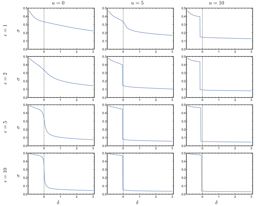
Figure 1: $\sigma$ vs $\delta$, for different given values of persistence length $\epsilon$ (rows) and self - avoidance strength $u$ (columns), the vertical gray dashed line marks the case of a sphere ($\delta=0$). Longer persistence lengths drive the system into higher order along the large dimension of the ellipsoid. Stronger self - avoidance, however, both adds a metastable state (not shown, see appendix B), and drive the lowest energy state into order along the poles. This is a purely entropic effect, caused by the existence of more ordered states along this direction. This happens even for oblate spheroids ($\delta<0$). The $\delta=0$ case, corresponding to a sphere, should be viewed here as as the limit $\delta\rightarrow 0$, since the treatment here assumes a broken symmetry (axial and not spherical).

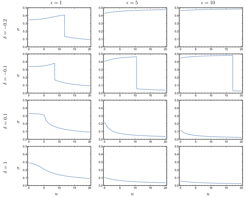
Figure 2: $\sigma$ vs $u$, for a given flattening $\delta$ (rows), and persistence lengths $\epsilon$ (columns). In strong self - avoidance, the system is driven into a polar oriented configuration even for oblate spheroids. In this case it’s an abrupt (first order) transition, due to entropy.

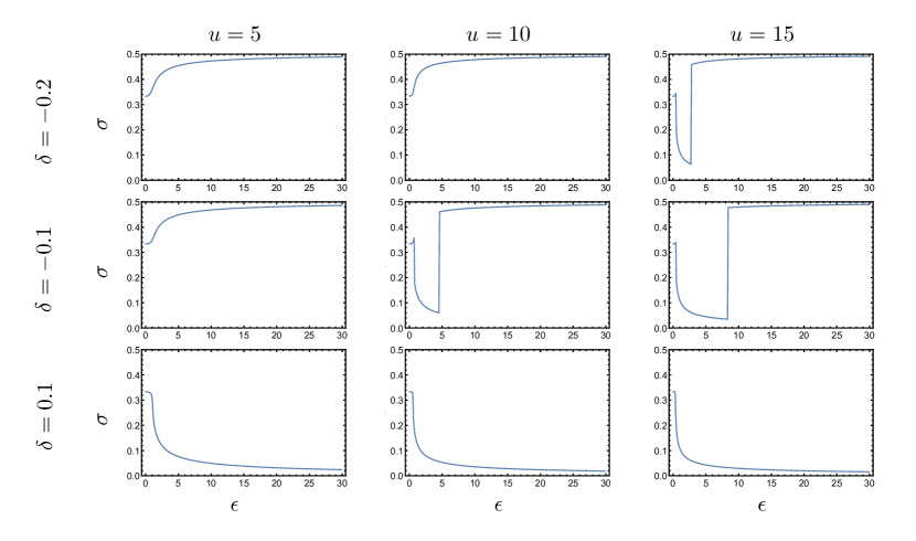
Figure 3: $\sigma$ vs $\epsilon$, for different given values of flattening $\delta$ (rows) and self avoidance $u$ (columns). The longer the persistence length is, the more energy (rather than entropy) is important, and the filaments align with the principal axis of the ellipsoid. Specifically, for $\delta<0$ this transition (from entropy dominated to energy dominated) is of first order.

Formally, Eq. (45) may have up to 5 solutions, however only up to 3 are physical (one is the ground state solution, one metastable and one unstable), satisfying the constraint $0\leq\sigma\leq\frac{1}{2}$. Fig. 4 depicts the critical surface $u^{*}(\epsilon,\delta)$. For any $u<u^{*}$ there is only one (stable) solution, while for $u>u^{*}$ there are three solutions (two are locally stable, one is unstable).

Additionally, we consider a completely random filament over the ellipsoid, to eliminate effects that relate only to the geometry of the surface rather that the elastic and entropic response of the filament to that geometry. A direct calculation of this dependence (see appendix C) yields

$$\sigma_{rand}=\frac{\sqrt{\delta\left(2+\delta\right)}\left[\delta\left(2+\delta\right)-1\right]+\left(1+\delta\right)^{4}\arccos\left(\frac{1}{1+\delta}\right)}{4\delta\left(2+\delta\right)\left[\sqrt{\delta\left(2+\delta\right)}+\left(1+\delta\right)^{2}\arccos\left(\frac{1}{1+\delta}\right)\right]}.$$

$\sigma_{rand}$ is plotted in Fig. 5. As clearly seen, at the $\delta\rightarrow-1$ limit $\sigma_{rand}\rightarrow\frac{1}{2}$. At this limit the (oblate) spheroid turns into a disc on the X-Y plane, which is in accordance with the result. At the $\delta\rightarrow\infty$ limit the spheroid is actually a cylinder, in which case the expected value for $\sigma_{rand}$, is $\sigma_{rand}(\infty)=\frac{1}{4}$. From Fig. 5 it is clear that the effects seen in Figures 1 - 3 are not simply geometric, and are related to the energy and entropy of the configuration, as the value of $\sigma$ is driven below $\sigma_{rand}$.

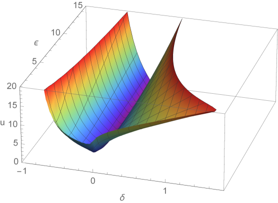
Figure 4: Critical surface. The volume above this surface describes the region in parameter space, where there are 3 physical solutions (one stable, one metastable, and one unstable), while underneath it there is only one (stable) solution. Note that this surface is infinite (for every $\delta$ and $\epsilon$ there is $u^{*}$ above which there are 3 solution.

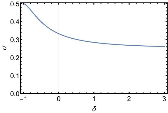
Figure 5: The global order parameter $\sigma_{rand}=\frac{\sqrt{\delta\left(2+\delta\right)}\left[\delta\left(2+\delta\right)-1\right]+\left(1+\delta\right)^{4}\arccos\left(\frac{1}{1+\delta}\right)}{4\delta\left(2+\delta\right)\left[\sqrt{\delta\left(2+\delta\right)}+\left(1+\delta\right)^{2}\arccos\left(\frac{1}{1+\delta}\right)\right]}$ of a randomly oriented director field on the surface of an ellipsoid, as function of $\delta$. $\sigma_{rand}\left(\delta\rightarrow-1\right)=\frac{1}{2}$ as expected from a random director field on a disc. $\sigma_{rand}\left(\delta\rightarrow\infty\right)=\frac{1}{4}$ as expected from a random director field on a cylinder.

The transitions described here are expected to affect the physical response and behavior of such systems. E.g. - the filament imposes stresses on the surface and may deform it. Therefore, we calculated the pressure $P$ exerted by the filament on the ellipsoid which is coupled to a change in area, the shear force $T$ which is coupled to a change in the flattening, and the injection force $F$ needed to further inject the filament into the ellipsoid. For solutions of Eq. (45), one can express the energy $W$:

$$W= \frac{\sqrt{2\pi}L}{16\sqrt{A}\epsilon}\left\{\frac{1}{\left(1-2\sigma\right)^{2}}+\frac{1}{\sigma^{2}}-8u\epsilon\left(1-2\sigma\right)\left(1-9\sigma\right)\right.$$ (48)

$$\left.+8\epsilon^{2}\left[6\sigma\left(\Sigma_{1}-\Sigma_{3}\right)+3\Sigma_{3}-\left(\sqrt{\Sigma_{1}}+\sqrt{\Sigma_{3}}\right)\right]\left[2\sigma\left(\Sigma_{1}-\Sigma_{3}\right)+\Sigma_{3}\right]\right\}$$

$$= \frac{\sqrt{2\pi}L}{16\sqrt{A}\epsilon}\mathcal{W}$$

where we defined $\mathcal{W}$ as the energy density per unit length of the filament.

The pressure $P$, exerted by the filament on the spheroid walls, is given by:

$$P= \frac{dW}{dA}=\frac{\sqrt{2\pi}L}{16\sqrt{A}\epsilon}\frac{d\mathcal{W}}{dA}=-\frac{\sqrt{2\pi}L}{32\sqrt{A^{3}}\epsilon}\left(\frac{d\mathcal{W}}{du}u+\frac{d\mathcal{W}}{d\epsilon}\epsilon\right),$$ (49)

where $\frac{d\mathcal{W}}{du}=\frac{\partial\mathcal{W}}{\partial u}+\frac{\partial\mathcal{W}}{\partial\sigma}\frac{d\sigma}{du}$ and similarly for $\epsilon$. In fig.6 we plot the pressure for a prolate ($\delta=0.1$, left) and oblate ($\delta=-0.1$, right) spheroid, as a function of the ellipsoid scale $\ell=\sqrt{\frac{A}{2\pi}}$, for given $\tilde{u}=1$, $\tilde{\epsilon}=1$, and $L=10$. Due to the scaling of the problem, as $\ell$ gets larger we simultaneously increase $u$ and decrease $\epsilon$. For this set of parameters, $\ell=1$ corresponds to an ellipsoid whose length - scale is similar to the persistence length, and thus breakage of the mean - field approximation. Other values result in similar looking graphs, though naturally the exact numbers change. For the case of $\delta=-0.1$, a small jump in pressure is seen. This jump corresponds to the snap-through of the configuration from an azimuthal order ($\sigma\sim 0.5$) for small $\ell$’s to polar order ($\sigma\sim 0$), when entropy governs the behaviour.

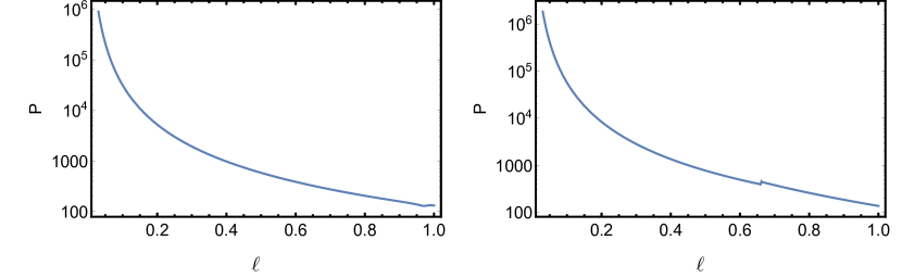
Figure 6: Pressure (Eq. (49)), exerted on the ellipsoid by the filament, of the stable solution as function of spheroid scale $\ell=\sqrt{\frac{A}{2\pi}}$. Left: $\delta=0.1$, right: $\delta=-0.1$. In both graphs $L=10$, $\tilde{u}=1$ and $\tilde{\epsilon}=1$. The small jump in pressure in the right figure corresponds to the jump in stable solutions from polar-like ($\sigma\sim 0$) to equatorial-like($\sigma\sim 0.5)$ as $\ell$ gets closer to 1. Similar to the transitions that can be seen in figs.2 and 3, as $u$ and $\epsilon$ decrease.

The normalized elongation shear stress $T$:

$$T= -\frac{dW}{d\delta}=-\frac{\sqrt{2\pi}L}{16\sqrt{A}\epsilon}\frac{d\mathcal{W}}{d\delta},$$ (50)

it is plotted in fig.7 (right) as a function of $\delta$ alongside the free energy $W$ (left), for given $\tilde{u}=1$, $\tilde{\epsilon}=1$, and $L=10$. It is clearly seen that there are two $\delta$ values in which the configuration is stable to shear. One is at $\delta<0$ which corresponds to an azimuthal order, and one in for $\delta>0$ corresponding to polar order. These two shear-stable solutions, are divided by a cusp at some $\delta_{c}<0$ corresponding to the $\delta$ change in ground state. These results show that for $\delta>\delta_{c}$, if we allow the ellipsoid to change the flattening (and only that), it will change its shape to the locally minimizing one (assuming the filament ordering relaxes fast enough). The exact position of the local minima, as well as the cusp depend on the exact values of the problem, but the qualitative result remains the same. For vanishing $\tilde{u}$ the cusp turns into a local maximum.

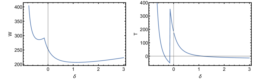
Figure 7: Left: Energy landscape (Eq. (48)) of the ground state as function of delta and Right: the corresponding shear stress (Eq. (50)) exerted on the ellipsoid to for deformations with same area. In both graphs $\tilde{u}=\tilde{\epsilon}=1$,$L=10$,$\ell=\frac{1}{2}$ which correspond to $u=6.36$ and $\epsilon=2$. Note a cusp in energy (and jump in shear stress) at the critical $\delta$ where the solution jumps from an equatorial-like ($\sigma\sim 0.5$) to polar-like ($\sigma\sim 0$). Additionally it clear that both for $\delta<0$ and $\delta>0$ there are some stable solutions. This

Finally, the injection force $F$ is given by

$$F= \frac{dW}{dL}=\frac{\sqrt{2\pi}}{16\sqrt{A}\epsilon}\mathcal{W}+\frac{\sqrt{2\pi}L}{16\sqrt{A}\epsilon}\frac{d\mathcal{W}}{dL}=\frac{\sqrt{2\pi}}{16\sqrt{A}\epsilon}\mathcal{W}+\frac{\sqrt{2\pi}u}{16\sqrt{A}\epsilon}\frac{d\mathcal{W}}{du}.$$ (51)

It is plotted in fig.8 for prolate ($\delta=0.1$, left) and oblate ($\delta=-0.1$, right) spheroids, as a function of the filament length $L$, for given $\ell=\sqrt{\frac{A}{2\pi}}=\frac{1}{2}$, $\tilde{u}=1$, and $\tilde{\epsilon}=1$. As $L$ gets larger we increase $u$, we therefore see that in the case of an oblate spheroid, at a long enough filament, a jump is observed in the configuration and respectively in the injection force, as the filament changes it’s configuration into a polar one at high densities (entropy driven snap-through). Other values of $\ell$, $\tilde{u}$ and $\tilde{\epsilon}$, and $\delta$ result in similar looking graphs, though naturally the exact numbers change. In the case of vanishing $\tilde{u}$ no jump is seen as the problem is only energetically driven.

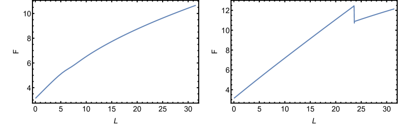
Figure 8: Force (Eq. (51)) needed to push further filament into the ellipsoid, of the stable solution as function of total length inside $L$. Left: $\delta=0.1$, right: $\delta=-0.1$. In both graphs $\ell=\frac{1}{2}$ ($A=\frac{\pi}{4}$), $\tilde{u}=1$ and $\tilde{\epsilon}=1\Rightarrow\epsilon=2$. The jump in pressure in the right figure corresponds to the jump in stable solutions from equatorial-like($\sigma\sim 0.5)$ to polar-like ($\sigma\sim 0$) as $L$ gets larger. Similar to the transitions that can be seen in figs.2 as $u$ increases.

IV Discussion

The results presented in this paper show the statistics of self avoiding semi-flexible filaments packed on the surface of ellipsoids. We find that geometry plays a significant role in the orientation of the filaments, and that without self avoidance, filaments tend to naturally order along the large dimension of the ellipsoid. This result is expected intuitively and support results in [1]. Self avoidance adds both energetic and entropic effects that give rise to surprising metastable solutions, and a rich behaviour of filament ordering. Most notably, an entropy induced snap-through transition is expected as when varying the ellipsoid’s aspect ratio, such entropic effects were described in the packing of DNA inside bacteria [48].

Despite describing the order of the filaments using an order parameter $\sigma$, that fact it is a global, rather than a local, measure means this work lacks a detailed description of the ordering. Thus it is hard to compare it to works such as those in [49, 50, 51, 52]. Nevertheless, an important difference is that the filament length in the system under study here is very long, which stand in contrast to the expected behavior of short segments, the latter should behave similar to nematics. Finite length effect were not taken into account here and are likely, at least in low - intermediate densities to play a role, especially, in filaments whose length is comparable to the ellipsoids size.

It is worth noting that at high persistence lengths, a transition reminiscent of the one suggested in [1] can be seen. As a function of $\delta$, we find a minimal value of $\sigma$, beyond which, as $\delta$ grows, $\sigma$ rises again. The main difference between this observation, and the transition originally suggested, is that this observation is a smooth and not an abrupt transition. This result suggests that the high curvature at the poles indeed plays some role in any actual configuration that might be observed. Namely, that filament configurations try to avoid the poles for high $\delta$’s.

To conclude, this paper suggests that geometry plays a significant, and often overlooked, mechanism of alignment of filaments inside unisotropic containers. The results shown here stand on their own, but are also complimentary to those presented in [1], treating more complicated cases (such as self avoidance) but without a direct expression of possible configurations. This suggests that geometry plays a significant role in packing of filaments inside non-isotropic containers, and serves both as an additional information to be included in other approaches, and as a foundation to study similar problems, and more complicated systems.

Residual stress, from forcing the filament into a curved shape (rather than a straight one) plays a significant role in these systems. Naturally bent filament affect the nature of this residual stress, and are likely to give much different results.

Finally, this work does not deal with asymmetric spheroids or other shapes, charged filaments, dynamics, and is limited to the mean - field approximation. As such there is much more work to be done. The addition of friction for example will likely produce hysteresis depending on the exact way in which filaments were introduced into the volume. Attempting to advance beyond the mean-field approximation will yield information regarding the configuration of the filaments.

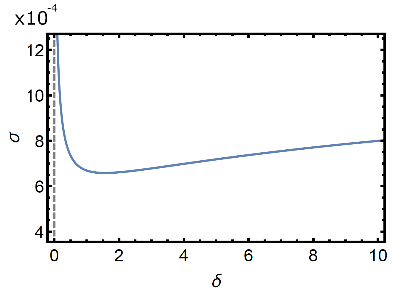
Figure 9: $\sigma$ as function of $\delta$ for $u=0$, $\epsilon=10,000$, approximating the limit of pure cold, non - self - avoiding filaments. The fact that $\sigma$ has a local minimum at small $\delta$’s suggests that a transition similar to the one described in [1] occurs.

To conclude, this paper suggests that geometry plays a significant, and often overlooked, mechanism of alignment of filaments inside unisotropic containers. The results shown here stand on their own, but are also complimentary to those presented in [1], treating more complicated cases (such as self avoidance) but without a direct expression of possible configurations. This suggests that geometry plays a significant role in packing of filaments inside non-isotropic containers, and serves both as an additional information to be included in other approaches, and as a foundation to study similar problems, and more complicated systems. Entropy is

Appendix A Detailed Calculations

Note that integrals of the form

$$\int\limits_{0}^{\infty}\frac{\,\text{d}q}{\tilde{\epsilon}q^{4}/2+(\lambda+\psi)q^{2}+\chi}=\frac{1}{\tilde{\epsilon}}\int\limits_{-\infty}^{\infty}\frac{\,\text{d}q}{q^{4}+2(\lambda^{\prime}+\psi^{\prime})q^{2}+\chi^{\prime}}$$ (52)

$$=\frac{1}{\tilde{\epsilon}}\int\limits_{-\infty}^{\infty}\frac{\,\text{d}q}{\left(q-i\sqrt{\beta+\sqrt{\beta^{2}-\gamma}}\right)\left(q+i\sqrt{\beta+\sqrt{\beta^{2}-\gamma}}\right)\left(q-i\sqrt{\beta-\sqrt{\beta^{2}-\gamma}}\right)\left(q+i\sqrt{\beta-\sqrt{\beta^{2}-\gamma}}\right)}$$

where we defined $\lambda^{\prime}=\lambda/\tilde{\epsilon}$, $\psi^{\prime}=\psi/\tilde{\epsilon}$, $\chi^{\prime}=2\chi/\tilde{\epsilon}$, and $\beta=\lambda^{\prime}+\psi^{\prime}$, $\gamma=\chi^{\prime}$. Using the residue theorem we find that

$$\int\limits_{0}^{\infty}\frac{\,\text{d}q}{\tilde{\epsilon}q^{4}/2+(\lambda+\psi)q^{2}+\chi} =\frac{\pi}{\sqrt{2\chi}\left(\sqrt{\lambda+\psi+\sqrt{(\lambda+\psi)^{2}-2\tilde{\epsilon}\chi}}+\sqrt{\lambda+\psi-\sqrt{(\lambda+\psi)^{2}-2\tilde{\epsilon}\chi}}\right)}$$ (53)

$$\int\limits_{0}^{\infty}\frac{q^{2}\,\text{d}q}{\tilde{\epsilon}q^{4}/2+(\lambda+\psi)q^{2}+\chi} =\frac{\pi}{\sqrt{\tilde{\epsilon}}\left(\sqrt{\lambda+\psi+\sqrt{(\lambda+\psi)^{2}-2\tilde{\epsilon}\chi}}+\sqrt{\lambda+\psi-\sqrt{(\lambda+\psi)^{2}-2\tilde{\epsilon}\chi}}\right)}$$ (54)

Thus, we finally remain with the following mean-field equations-

$$\frac{1}{2}\sum\limits_{i}\left[\frac{\Sigma_{i}}{\sqrt{2\chi}\left(\sqrt{\lambda+\psi_{i}+\sqrt{(\lambda+\psi_{i})^{2}-2\tilde{\epsilon}\chi\Sigma_{i}}}+\sqrt{\lambda+\psi_{i}-\sqrt{(\lambda+\psi_{i})^{2}-2\tilde{\epsilon}\chi\Sigma_{i}}}\right)}\right]-\ell^{2} =0$$ (55)

$$\frac{1}{2}\sum\limits_{i}\left[\frac{1}{\sqrt{\tilde{\epsilon}}\left(\sqrt{\lambda+\psi_{i}+\sqrt{(\lambda+\psi_{i})^{2}-2\tilde{\epsilon}\chi\Sigma_{i}}}+\sqrt{\lambda+\psi_{i}-\sqrt{(\lambda+\psi_{i})^{2}-2\tilde{\epsilon}\chi\Sigma_{i}}}\right)}\right]-1 =0$$ (56)

$$\frac{L}{2}\left[\frac{1}{\sqrt{\tilde{\epsilon}}\left(\sqrt{\lambda+\psi_{i}+\sqrt{(\lambda+\psi_{i})^{2}-2\tilde{\epsilon}\chi\Sigma_{i}}}+\sqrt{\lambda+\psi_{i}-\sqrt{(\lambda+\psi_{i})^{2}-2\tilde{\epsilon}\chi\Sigma_{i}}}\right)}\right]-A\sigma_{i} =0$$ (57)

$$-\psi_{i}+\tilde{u}\left((\sigma_{1}+\sigma_{2}+\sigma_{3})-\sigma_{i}\right) =0.$$ (58)

By defining $z_{i}=\sqrt{\lambda+\psi_{i}+\sqrt{(\lambda+\psi_{i})^{2}-2\tilde{\epsilon}\chi\Sigma_{i}}}$ and $\bar{z}_{i}=\sqrt{\lambda+\psi_{i}-\sqrt{(\lambda+\psi_{i})^{2}-2\tilde{\epsilon}\chi\Sigma_{i}}}$, and using the fact that $\sigma_{1}+\sigma_{2}+\sigma_{3}=1$ and $\sigma_{1}=\sigma_{2}$ we get

$$\frac{1}{2\sqrt{2\chi}}\left[\frac{2\Sigma_{1}}{z_{1}+\bar{z}_{1}}+\frac{\Sigma_{3}}{z_{3}+\bar{z}_{3}}\right]-\ell^{2} =0$$ (59)

$$\frac{1}{2\sqrt{\tilde{\epsilon}}}\left[\frac{2}{z_{1}+\bar{z}_{1}}+\frac{1}{z_{3}+\bar{z}_{3}}\right]-1 =0$$ (60)

$$\frac{L}{2\sqrt{\tilde{\epsilon}}}\frac{1}{z_{i}+\bar{z}_{i}}-Ac\sigma_{i} =0$$ (61)

$$-\psi_{i}+\tilde{u}c\left(1-\sigma_{i}\right) =0$$ (62)

which we can further simplified into dimensionless quantities by dividing Eq. (A8) by $\ell^{2}$ and Eq. (A10) by $Ac$

$$\frac{1}{2\ell^{2}\sqrt{2\chi}}\left[\frac{2\Sigma_{1}}{z_{1}+\bar{z}_{1}}+\frac{\Sigma_{3}}{z_{3}+\bar{z}_{3}}\right]-1 =0$$ (63)

$$\frac{1}{2\sqrt{\tilde{\epsilon}}}\left[\frac{2}{z_{1}+\bar{z}_{1}}+\frac{1}{z_{3}+\bar{z}_{3}}\right]-1 =0$$ (64)

$$\frac{1}{2\sqrt{\tilde{\epsilon}}}\frac{1}{z_{i}+\bar{z}_{i}}-\sigma_{i} =0$$ (65)

$$-\psi_{i}+\tilde{u}c\left(1-\sigma_{i}\right) =0$$ (66)

Inserting equations (A14) is equation (A12)

$$1 =\frac{\sqrt{\tilde{\epsilon}}}{\ell^{2}\sqrt{2\chi}}\left[2\sigma(\Sigma_{1}-\Sigma_{3})+\Sigma_{3}\right]$$ (67)

multiplying by $$\sqrt{2\chi}$$

$$\sqrt{2\chi} =\frac{\sqrt{\tilde{\epsilon}}}{\ell^{2}}\left[2\sigma(\Sigma_{1}-\Sigma_{3})+\Sigma_{3}\right]$$ (68)

squaring both sides and dividing by $$2$$, we find

$$\chi =\frac{{\tilde{\epsilon}}}{2\ell^{4}}\left[2\sigma(\Delta\Sigma)+\Sigma_{3}\right]^{2}$$ (69)

where we marked $\Delta\Sigma=\Sigma_{1}-\Sigma_{3}$. From Eq. (A14) we also get-

$$z_{1}+\bar{z}_{1} =\frac{1}{2\sqrt{\tilde{\epsilon}}\sigma}$$ (70)

taking the square on both sides yields

$$z_{1}^{2}+\bar{z}_{1}^{2}+2z_{1}\bar{z}_{1} =\frac{1}{4\tilde{\epsilon}\sigma^{2}}$$ (71)

which we can write explicitly

$$2\left(\lambda+\tilde{u}c(1-\sigma)+\sqrt{2\tilde{\epsilon}\chi\Sigma_{1}}\right) =\frac{1}{4\tilde{\epsilon}\sigma^{2}}$$ (72)

$$\lambda+\tilde{u}c(1-\sigma)+\sqrt{2\tilde{\epsilon}\chi\Sigma_{1}} =\frac{1}{8\tilde{\epsilon}\sigma^{2}}$$ (73)

and finally we can isolate $$\lambda$$

$$\lambda =\frac{1}{8\tilde{\epsilon}\sigma^{2}}-uc(1-\sigma)-\frac{\tilde{\epsilon}}{\ell^{2}}\sqrt{\Sigma_{1}}\left[2\sigma\Delta\Sigma+\Sigma_{3}\right].$$ (74)

Following the same process for $z_{3}$ we get

$$\lambda =\frac{1}{8\tilde{\epsilon}(1-2\sigma)^{2}}-2u\tilde{u}\sigma-\frac{\tilde{\epsilon}}{\ell^{2}}\sqrt{\Sigma_{3}}\left[2\sigma\Delta\Sigma+\Sigma_{3}\right].$$ (75)

As these equations (A23) and (A24) are of the same variable, we can equate both right hand sides to get a sn equation for $\sigma$:

$$\frac{1}{8\tilde{\epsilon}\sigma^{2}}-\frac{1}{8\tilde{\epsilon}(1-2\sigma)^{2}}-\tilde{u}c(1-3\sigma)-\frac{\tilde{\epsilon}}{\ell^{2}}\left(\sqrt{\Sigma_{1}}-\sqrt{\Sigma_{3}}\right)\left[2\sigma\left(\Sigma_{1}-\Sigma_{3}\right)+\Sigma_{3}\right] =0.$$ (76)

Appendix B Metastable state

As Eq.(45) may have more than one solution, stability classification was needed. Being an effective equation, stability analysis was done directly from this equation, using standard techniques borrowed from catastrophe theory, as explained in the the main text. We thus plot the same graphs as in 1 - 3, this time not only with the most stable solution, rather with the unstable (green dash-dotted) and meta-stable (yellow dashed) curves.

In fig.10 we see $\sigma$ plotted against the flattening $\delta$ for various values of $u$, $\epsilon$. Most notably we see that whenever the ground state appears to abruptly change, we find that in a neighbourhood about it there are 3 solutions rather than a single. An unstable solution always appear near $\sigma\sim\frac{1}{3}$. Most importantly we see that the existence region of the metastable states gets larger with the self avoidance $u$.

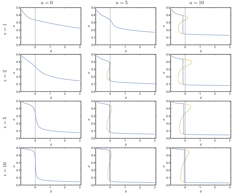
Figure 10: $\sigma$ vs $\delta$, for different given values of $\epsilon$ (rows) and $u$ columns, the vertical gray dashed line marks the case of a sphere. Notice that since we assume a cylindrical symmetry in our analysis, even in perfect sphere case we get a distinct stable state. The results at $\delta=0$ should be understood as corresponding to the limit $\delta\rightarrow 0$ (i.e. - the limit of an infinitesimally broken symmetry). The region between this (gray) line and the vertical drop is the region of where entropy prevails over the energy for the oblate spheroid.

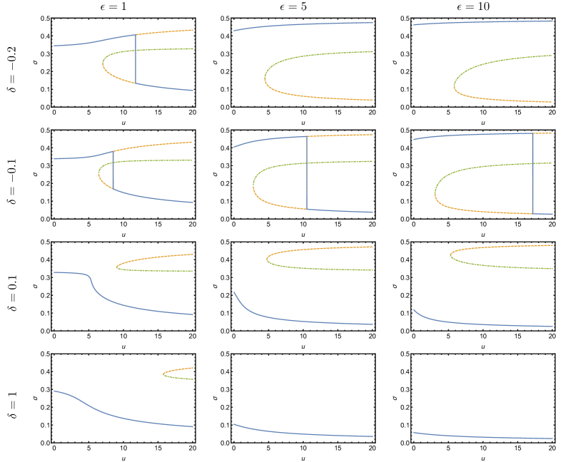
Figure 11: $\sigma$ vs $u$, for a given $\delta$, $\epsilon$.

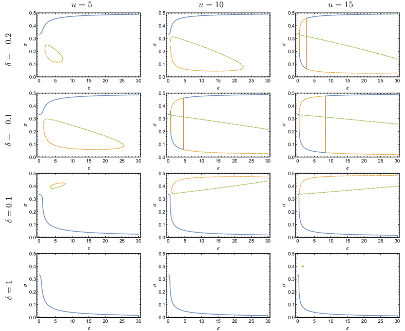
Figure 12: $\sigma$ vs $\epsilon$, for different given values of $\delta$ (rows) and $u$ columns.

Appendix C Random coil

Calculation of the random coil is done first by describing the configuration of an ellipsoid, using polar coordinates $\theta m,\phi$ :

$$\mathbf{f}\left(\theta,\phi\right)=\left\{\cos\phi\sin\theta,\sin\phi\sin\theta,\left(1+\delta\right)\cos\theta\right\}.$$

Here $\delta$ is the flattening. Note that the axes scaling is constant, and does not change with $\delta$ as we eventually average over the area, and it does not play a role.

We can now define a locally flat frame $\mathbf{t}_{\theta}=\frac{\partial_{\theta}\mathbf{f}}{\sqrt{\partial_{\theta}\mathbf{f}\cdot\partial_{\theta}\mathbf{f}}}$, $\mathbf{t}_{\phi}=\frac{\partial_{\phi}\mathbf{f}}{\sqrt{\partial_{\phi}\mathbf{f}\cdot\partial_{\phi}\mathbf{f}}}$ ,$\hat{\mathbf{n}}=\frac{\mathbf{t}_{\theta}\times\mathbf{f}_{\phi}}{\left|\mathbf{t}_{\theta}\times\mathbf{t}_{\phi}\right|}$. Where $\mathbf{t}_{\theta}$ and $\mathbf{t}_{\phi}$ are the surface tangents and $\hat{\mathbf{n}}$ is the normal. A ”2D” unit vector locally given by $r=\left(\cos\psi,\sin\psi\right)$ (where $\psi$ is the angle relative to $\mathbf{t}_{\theta}$ has the 3D form

$$\mathbf{r}_{3D}=\cos\psi\mathbf{t}_{\theta}+\sin\psi\mathbf{t}_{\phi}.$$ (77)

The orientation vector $\sigma_{\mu\nu}(\psi,\theta,\phi)$ is then given by $\sigma^{\mu\nu}=r_{3D}^{\mu}r_{3D}^{\nu}$. The global, averaged tensor is then given by:

$$\sigma_{glob}^{\mu\nu}=\frac{\int\left(\int r_{3D}^{\mu}r_{3D}^{\nu}\,\text{d}\psi\right)\sqrt{\sin^{2}\theta\left(\cos^{2}\theta\left(1+\delta\right)^{2}\sin^{2}\theta\right)}\,\text{d}\theta\,\text{d}\phi}{2\pi\int\sqrt{\sin^{2}\theta\left(\cos^{2}\theta\left(1+\delta\right)^{2}\sin^{2}\theta\right)}\,\text{d}\theta\,\text{d}\phi}.$$ (78)

Comparing the result to the form $\left(\begin{array}[]{ccc}\sigma_{rand}&0&0\\ 0&\sigma_{rand}&0\\ 0&&1-2\sigma_{rand}\end{array}\right)$, we find

$$\sigma_{rand}=\frac{\sqrt{\delta\left(2+\delta\right)}\left[\delta\left(2+\delta\right)-1\right]+\left(1+\delta\right)^{4}\arccos\left(\frac{1}{1+\delta}\right)}{4\delta\left(2+\delta\right)\left[\sqrt{\delta\left(2+\delta\right)}+\left(1+\delta\right)^{2}\arccos\left(\frac{1}{1+\delta}\right)\right]}.$$

References

- Grossman et al. [2021] D. Grossman, E. Katzav, and E. Sharon, Packing of stiff rods on ellipsoids: Geometry, Physical Review E 103, 013001 (2021).
- Uyttewaal et al. [2012] M. Uyttewaal, A. Burian, K. Alim, B. Landrein, D. Borowska-Wykrrt, A. Dedieu, A. Peaucelle, M. Ludynia, J. Traas, A. Boudaoud, et al., Mechanical stress acts via katanin to amplify differences in growth rate between adjacent cells in arabidopsis, Cell 149, 439 (2012).
- Burk and Ye [2002] D. H. Burk and Z.-H. Ye, Alteration of oriented deposition of cellulose microfibrils by mutation of a katanin-like microtubule-severing protein, The Plant Cell 14, 2145 (2002).
- Stoop [2011] N. B. Stoop, Morphogenesis in constrained spaces, Ph.D. thesis, ETH Zurich (2011).
- Marenduzzo et al. [2010] D. Marenduzzo, C. Micheletti, and E. Orlandini, Biopolymer organization upon confinement, Journal of Physics: Condensed Matter 22, 283102 (2010).
- Katzav et al. [2006] E. Katzav, M. Adda-Bedia, and A. Boudaoud, A statistical approach to close packing of elastic rods and to dna packaging in viral capsids, Proceedings of the National Academy of Sciences 103, 18900 (2006).
- Boué and Katzav [2007] L. Boué and E. Katzav, Folding of flexible rods confined in 2d space, EPL (Europhysics Letters) 80, 54002 (2007).
- Purohit et al. [2003a] P. K. Purohit, J. Kondev, and R. Phillips, Mechanics of dna packaging in viruses, Proceedings of the National Academy of Sciences 100, 3173 (2003a).
- Vetter et al. [2013] R. Vetter, F. Wittel, N. Stoop, and H. Herrmann, Finite element simulation of dense wire packings, European Journal of Mechanics-A/Solids 37, 160 (2013).
- Vetter [2015] R. Vetter, Growth, interaction and packing of thin objects, Ph.D. thesis, ETH Zurich (2015).
- Pineirua et al. [2013] M. Pineirua, M. Adda-Bedia, and S. Moulinet, Spooling and disordered packing of elastic rods in cylindrical cavities, EPL (Europhysics Letters) 104, 14005 (2013).
- Elettro [2015] H. Elettro, Elastocapillary windlass: from spider silk to smart actuators, Ph.D. thesis (2015).
- Elettro et al. [2017a] H. Elettro, F. Vollrath, A. Antkowiak, and S. Neukirch, Drop-on-coilable-fibre systems exhibit negative stiffness events and transitions in coiling morphology, Soft matter 13, 5509 (2017a).
- Elettro et al. [2017b] H. Elettro, P. Grandgeorge, and S. Neukirch, Elastocapillary coiling of an elastic rod inside a drop, Journal of Elasticity 127, 235 (2017b).
- Elsner et al. [2012] J. Elsner, M. Michalski, and D. Kwiatkowska, Spatiotemporal variation of leaf epidermal cell growth: a quantitative analysis of arabidopsis thaliana wild-type and triple cyclind3 mutant plants, Annals of botany 109, 897 (2012).
- Efrati et al. [2009] E. Efrati, E. Sharon, and R. Kupferman, Buckling transition and boundary layer in non-Euclidean plates, Phys. Rev. E 80, 016602 (2009).
- Aharoni et al. [2014] H. Aharoni, E. Sharon, and R. Kupferman, Geometry of thin nematic elastomer sheets, Physical review letters 113, 257801 (2014).
- Armon et al. [2011] S. Armon, E. Efrati, R. Kupferman, and E. Sharon, Geometry and Mechanics in the Opening of Chiral Seed Pods, Science 333, 1726 (2011).
- Grossman et al. [2016] D. Grossman, E. Sharon, and H. Diamant, Elasticity and fluctuations of frustrated nanoribbons, Phys. Rev. Lett. 116, 258105 (2016).
- Grossman et al. [2018] D. Grossman, E. Sharon, and E. Katzav, Shape and fluctuations of positively curved ribbons, Physical Review E 98, 022502 (2018).
- Fisher and Cyr [1998] D. D. Fisher and R. J. Cyr, Extending the microtubule/microfibril paradigm: cellulose synthesis is required for normal cortical microtubule alignment in elongating cells, Plant Physiology 116, 1043 (1998).
- Somerville et al. [2004] C. Somerville, S. Bauer, G. Brininstool, M. Facette, T. Hamann, J. Milne, E. Osborne, A. Paredez, S. Persson, T. Raab, et al., Toward a systems approach to understanding plant cell walls, Science 306, 2206 (2004).
- Sahaf and Sharon [2016] M. Sahaf and E. Sharon, The rheology of a growing leaf: stress-induced changes in the mechanical properties of leaves, Journal of experimental botany 67, 5509 (2016).
- Oh et al. [2014] E. Oh, J.-Y. Zhu, M.-Y. Bai, R. A. Arenhart, Y. Sun, and Z.-Y. Wang, Cell elongation is regulated through a central circuit of interacting transcription factors in the arabidopsis hypocotyl, elife 3, e03031 (2014).
- Chaiwanon et al. [2016] J. Chaiwanon, W. Wang, J.-Y. Zhu, E. Oh, and Z.-Y. Wang, Information integration and communication in plant growth regulation, Cell 164, 1257 (2016).
- De Frutos et al. [2005] M. De Frutos, L. Letellier, and E. Raspaud, Dna ejection from bacteriophage t5: analysis of the kinetics and energetics, Biophysical journal 88, 1364 (2005).
- Purohit et al. [2003b] P. K. Purohit, J. Kondev, and R. Phillips, Force steps during viral dna packaging?, Journal of the Mechanics and Physics of Solids 51, 2239 (2003b).
- Purohit et al. [2005] P. K. Purohit, M. M. Inamdar, P. D. Grayson, T. M. Squires, J. Kondev, and R. Phillips, Forces during bacteriophage dna packaging and ejection, Biophysical journal 88, 851 (2005).
- Kindt et al. [2001] J. Kindt, S. Tzlil, A. Ben-Shaul, and W. M. Gelbart, Dna packaging and ejection forces in bacteriophage, Proceedings of the National Academy of Sciences 98, 13671 (2001).
- Smith et al. [2001] D. E. Smith, S. J. Tans, S. B. Smith, S. Grimes, D. L. Anderson, and C. Bustamante, The bacteriophage 29 portal motor can package dna against a large internal force, Nature 413, 748 (2001).
- Fathizadeh et al. [2013] A. Fathizadeh, M. Heidari, B. Eslami-Mossallam, and M. R. Ejtehadi, Confinement dynamics of a semiflexible chain inside nano-spheres, The Journal of chemical physics 139, 044912 (2013).
- Nikoubashman et al. [2017] A. Nikoubashman, D. A. Vega, K. Binder, and A. Milchev, Semiflexible polymers in spherical confinement: Bipolar orientational order versus tennis ball states, Physical review letters 118, 217803 (2017).
- Milchev et al. [2018] A. Milchev, S. A. Egorov, A. Nikoubashman, and K. Binder, Adsorption and structure formation of semiflexible polymers on spherical surfaces, Polymer 145, 463 (2018).
- Netz and Andelman [2003] R. R. Netz and D. Andelman, Neutral and charged polymers at interfaces, Physics reports 380, 1 (2003).
- Borukhov et al. [1997] I. Borukhov, D. Andelman, and H. Orland, Steric effects in electrolytes: A modified poisson-boltzmann equation, Physical review letters 79, 435 (1997).
- Abrashkin et al. [2007] A. Abrashkin, D. Andelman, and H. Orland, Dipolar poisson-boltzmann equation: ions and dipoles close to charge interfaces, Physical review letters 99, 077801 (2007).
- Slosar and Podgornik [2006] A. Slosar and R. Podgornik, On the connected-charges thomson problem, EPL (Europhysics Letters) 75, 631 (2006).
- van der Schoot and Bruinsma [2005] P. van der Schoot and R. Bruinsma, Electrostatics and the assembly of an rna virus, Physical Review E 71, 061928 (2005).
- Ghosh et al. [2002] K. Ghosh, G. Carri, and M. Muthukumar, Phase transitions in solutions of semiflexible polyelectrolytes, The Journal of chemical physics 116, 5299 (2002).
- Carri and Muthukumar [1999] G. A. Carri and M. Muthukumar, Attractive interactions and phase transitions in solutions of similarly charged rod-like polyelectrolytes, The Journal of chemical physics 111, 1765 (1999).
- Edwards [1965] S. F. Edwards, The statistical mechanics of polymers with excluded volume, Proceedings of the Physical Society 85, 613 (1965).
- Newton [1726] I. Newton, Philosophiae naturalis principia mathematica, Vol. 3 (Apud Guil. & Joh. Innys, Regiæ Societatis typographos, 1726).
- Bessel [1825] F. Bessel, ” uber die berechnung der geographischen l” angen und breiten aus geod” atischen vermessungen, Astronomische Nachrichten 4, 241 (1825).
- Bessel et al. [2009] F. Bessel, C. F. Karney, and R. E. Deakin, The calculation of longitude and latitude from geodesic measurements, arXiv preprint arXiv:0908.1824 (2009).
- Saunders [1980] P. T. Saunders, An introduction to catastrophe theory (Cambridge University Press, 1980).
- Misbah [2016] C. Misbah, Complex Dynamics and Morphogenesis (Springer, 2016).
- Chirilus-Bruckner et al. [2015] M. Chirilus-Bruckner, A. Doelman, P. van Heijster, and J. D. Rademacher, Butterfly catastrophe for fronts in a three-component reaction–diffusion system, Journal of Nonlinear Science 25, 87 (2015).
- Jun and Mulder [2006] S. Jun and B. Mulder, Entropy-driven spatial organization of highly confined polymers: lessons for the bacterial chromosome, Proceedings of the National Academy of Sciences 103, 12388 (2006).
- MacKintosh and Lubensky [1991] F. MacKintosh and T. Lubensky, Orientational order, topology, and vesicle shapes, Physical review letters 67, 1169 (1991).
- Lubensky and Prost [1992] T. Lubensky and J. Prost, Orientational order and vesicle shape, Journal de Physique II 2, 371 (1992).
- Evans [1995] R. Evans, Phase diagrams for deformable toroidal and spherical surfaces with intrinsic orientational order, Journal de Physique II 5, 507 (1995).
- Vitelli and Nelson [2006] V. Vitelli and D. R. Nelson, Nematic textures in spherical shells, Physical Review E 74, 021711 (2006).