Deep Algebraic Fitting for Multiple Circle Primitives Extraction from Raw Point Clouds

Abstract

The shape of circle is one of fundamental geometric primitives of man-made engineering objects. Thus, extraction of circles from scanned point clouds is a quite important task in 3D geometry data processing. However, existing circle extraction methods either are sensitive to the quality of raw point clouds when classifying circle-boundary points, or require well-designed fitting functions when regressing circle parameters. To relieve the challenges, we propose an end-to-end Point Cloud Circle Algebraic Fitting Network (Circle-Net) based on a synergy of deep circle-boundary point feature learning and weighted algebraic fitting. First, we design a circle-boundary learning module, which considers local and global neighboring contexts of each point, to detect all potential circle-boundary points. Second, we develop a deep feature based circle parameter learning module for weighted algebraic fitting, without designing any weight metric, to avoid the influence of outliers during fitting. Unlike most of the cutting-edge circle extraction wisdoms, the proposed classification-and-fitting modules are originally co-trained with a comprehensive loss to enhance the quality of extracted circles. Comparisons on the established dataset and real-scanned point clouds exhibit clear improvements of Circle-Net over SOTAs in terms of both noise-robustness and extraction accuracy. We will release our code, model, and data for both training and evaluation on GitHub upon publication.

1 Introduction

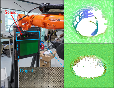
Figure 1: One of our inspection scenes, where noisy point clouds of multiple circles are captured. In the traditional geometric processing field, circle extraction from point clouds should be divided into two (individual) steps, i.e., classifying circle-boundary points, and fitting a series of circles from these classified circle-boundary points. However, the classification, i.e., judging whether a point is a circle-boundary point or not, is sensitive to the quality of raw point clouds, and the fitting step requires well-designed weighting functions when regressing circle parameters. Is it possible to combine the learning-based local feature representation and traditional algebraic fitting model together, to robustly and accurately fit circles in a deep learning fashion? This work answers the question by designing Circle-Net, an end-to-end Point Cloud Circle Algebraic Fitting Network.

Geometric primitive extraction from man-made engineering objects is essential for many practically meaningful applications, such as reverse engineering Lafarge and Mallet (2012) and 3D inspection Kleppe et al (2019). As very common circle primitives in aviation manufacturing, the repetitive rivet holes have an important effect on production quality control. Fig. 1 presents a practical circle inspection scene. Cutting-edge vision-based techniques have been developed to extract circles from either captured images or scanned point clouds (Wang et al (2020); Xie et al (2020)). Although possibly serving to determine the rivet hole’s quality, these methods still involve many parameters to fine-tune (i.e., complicated efforts on human-computer interactions) and are limited by their extraction accuracy Zhang et al (2021). More specifically, the calculation accuracy of existing methods varies from 0.03 $mm$ to 0.06 $mm$, which cannot meet the H accuracy requirement (0.02 $mm$) of standard rivet holes.

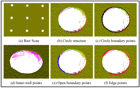
Figure 2: Circle-boundary points. (a) is the raw yet low-fidelity scan, and (b) is a circular structure in (a). The black points in (c) are the exact circle-boundary points. The pink points in (d) are inner-wall points scanned from the inside of the cylinder. In (e) and (f), the blue points and the red points are open boundary points and edge points respectively, which form the full boundary points of the circle in (c).

In the actual 3D measurement process, the acquired point clouds are usually incomplete and noisy, due to the surface reflection, self-occlusion, or limited scanning ranges. Hence, we define the circle-boundary point as the edge point or the open boundary point located around the boundary of a circle. To explain the defined circle-boundary point, we present an example of the real-scanned engineering object with multiple circles on it in Fig. 2. The pink points in Fig. 2 (d) are inner-wall points sampled from the surface of the cylinder of the target; the blue points in Fig. 2 (e) and the red points in Fig. 2 (f) form the full boundary points of the circle in Fig. 2 (c). Obviously, there always exists certain fitting error, even for human operators.

Circle extraction from point clouds mainly consists of two (individual) operations: (i) classifying initial circle-boundary points (i.e., determining whether each point in the point cloud is a circle-boundary point or not); and (ii) fitting a series of repetitive circles from these promising circle-boundary points. The main challenge in the first operation is that existing boundary/edge detection methods (Rusu and Cousins (2011); Gersho and Gray (2012); Belton and Lichti (2006); Yu et al (2018); Wang et al (2020); Chen et al (2021)) cannot effectively distinguish which points are boundary points of circles or not, since these circle primitives are usually distributed on the base surface as very plain features (i.e., subtle differences between the base surface and circles). For the latter operation which aims to compute accurate parameters of the circles, typical methods include weighted least-squares (WLS) fitting (Rousseeuw and Leroy (2005); Cleveland (1979); Nurunnabi et al (2015b)) and RANSAC-based solutions (Torr and Zisserman (2000)). However, the real-scanned point clouds of man-made engineering objects are often of low fidelity (e.g., biased noise, outliers, distortions, missing boundaries, or unclear boundaries), as shown in Fig. 1, even if acquired with a high-accuracy measurement devices such as Creaform MetraScan, and Wenglor MLAS202. Such low-fidelity data makes existing parameter estimation methods difficult to design weight functions to measure the significance of each point for accurately fitting a circle.

To this end, we propose to endow classical circle algebraic fitting with an adaptive weight learning mechanism, by cascading and synergizing the aforementioned two operations into a neural network. In detail, (1) we design a circle-boundary learning module, which considers local and global neighboring contexts of each point, to detect all potential circle-boundary points; (2) we develop a circle parameter learning module for algebraic circle fitting, without designing any weight metric to avoid the influence of outliers during fitting; (3) the classification-and-fitting modules are originally co-trained with a comprehensive loss to enhance the quality of extracted circles, which to our knowledge is the first time.

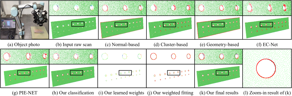
Figure 3: Comparison of circle-boundary point detection by different methods from a raw point cloud (scanned by a MetraSCAN 3D Scanner). (a) and (b) are the photo of a mechanical part and its corresponding real-scanned point cloud respectively. From (c) to (h): the circle-boundary point detection results by different methods, including normal-based Rusu and Cousins (2011), cluster-based Gersho and Gray (2012), geometry-based Belton and Lichti (2006), EC-NET Yu et al (2018), PIE-NET Wang et al (2020) and our classification network. (i) and (j) are our learned point-wise weights and the corresponding circle fitting results. (k) visualizes the fitted circles (j) in the raw point cloud (b). (l) highlights one circle for better observing our fitting results. Compared with other methods, our approach can detect circle-boundary points more reliably and produce circle primitives more accurately.

To summarize, the major features of our novel circle extraction method include:

• An end-to-end point cloud circle algebraic fitting network (Circle-Net) is proposed, which is a fully automatic multi-circle extraction paradigm for joint circle-boundary point classification and algebraic circle fitting.

• A transformer-based point classification network is proposed, which can detect all potential circle-boundary points from raw point clouds, while excluding the other kinds of boundary points.

• A circle parameter estimation network for raw point clouds is proposed, which predicts point-wise weights for weighted algebraic fitting of circles with artifacts, such as noise, outliers, shape distortion, and missing boundaries.

• An industrial application of quality inspection for the drilling circles is conducted, which further demonstrates the practicality of our proposed Circle-Net.

Through a variety of experiments, we show that our method significantly outperforms the state-of-the-art approaches, in terms of both circle-boundary point classification and circle fitting accuracy (Sec. 6), as demonstrated in Fig. 3.

2 Related Work

In this section, we review the related work from three aspects, that is, boundary point detection, robust circle fitting, and deep learning for unstructured point clouds.

2.1 Boundary point detection

It is a nontrivial task to identify the borderline and detect the boundary points from an unstructured point cloud. The human brain can determine the boundary of the point cloud by observing the distribution of the point cloud. For a computer, a point cloud is just vector data without a clear boundary. Barber et al. Barber et al (1996) propose the Quickhull method to detect the smallest convex polygon containing all points by a divide and conquer approach from a given set of finite bi-dimensional points. Their method is very effective, but it can only detect a set of boundary points belonging to the convex polygon. Akkiraju et al (1995) propose an alpha-shape method generalized from QuickHull, which can deal with concave areas and holes in point clouds. Kettner et al (2004) propose Computational Geometry Algorithms Library (CGAL) which implements alpha-shape for 2D and 3D point clouds robustly. However, the performance of the alpha-shape method is limited by the involved parameter and the point sampling irregularity. Öztireli et al (2009) give a non-parametric edge extraction method based on kernel regression. Bazazian et al (2015) propose a non-parametric method based on analysis of eigenvalue. Chen et al (2021) propose an effective multi-scale feature line extraction method, which can detect different levels of geometric features from noisy input with high accuracy. Mineo et al (2019) introduce an algorithm to boundary point detection and spatial filtering approach based on Fast Fourier Transform (FFT). This method generates low noise tessellated surfaces from point cloud data directly by detecting points belonging to sharp edges and creases which are not based on predefined threshold values. As we reviewed, most boundary detection methods are only suitable for the detection of sharp edges or boundaries, rather than detecting specific circle boundaries.

2.2 Circle fitting

Geometric and algebraic are the two main kinds of circle fitting methods. The geometric method minimizes the sum of the square distances from the data point to the circle and produces invariant results under rotations and translations Abdul-Rahman and Chernov (2014). Two classical geometric methods are Gauss-Newton and Levenberg-Marquardt Chernov (2010). Many later circle fitting approaches are inspired by them. For example, Calafiore (2002) propose to use a difference-of-squares as a geometric criterion to obtain a closed-form solution. Chernov and Lesort (2005) present an alternative Levenberg-Marquardt algorithm, and prove the superiority of this approach in terms of robustness, reliability, and efficiency. De Guevara et al (2011) propose an iterative geometric fitting using mean absolute error to reduce outlier influence. Generally speaking, geometric fitting is more accurate than algebraic fitting, even though it has intensive iterative computation. However, the initial guess seriously affects the results of geometric fitting (Chernov (2010); Al-Sharadqah (2014)). Specifically, Abdul-Rahman and Chernov (2014) think that the divergence probability of algebraic fitting is much lower than that of geometric fitting.

Algebraic fitting is non-iterative, faster, and provides a good initial guess. It minimizes the algebraic function. Chernov and Lesort (2005) propose using an algebraic method to determine algebraic parameters for the best fitting circle and then center and radius are obtained from them and converge to a minimum of the sum of the squared geometric distance. Kåsa (1976) proposes a simple and fast algebraic approach that is used as a basis by many circle fitting methods. The approach minimizes the square of radius, which is a linear least-squares problem and can be solved easily as a system of linear equations. Notably, Al-Sharadqah et al (2009) observe that the method introduced by Kåsa (1976) is heavily biased toward smaller circular arcs. Pratt (1987) and Taubin (1991) extend this. They each develop one popular method, which only needs to change the parameter constraints. Al-Sharadqah et al (2009) develop a method, called Hyper, by minimizing the algebraic function using the two constraints proposed by Pratt (1987) and Taubin (1991). Al-Sharadqah (2014) and Al-Sharadqah et al (2009) note that the Hyper approach outperforms many efficient existing algebraic methods, is nearly as good as some efficient geometric fittings, is useful for incomplete data, and has the correct estimate. Like Pratt (1987) and Taubin (1991), Hyper Al-Sharadqah et al (2009) produces invariant results under rotations and translations by using a constraint matrix, which is a linear combination of the two constraints of Pratt (1987) and Taubin (1991), that satisfies the invariance requirements (Chernov (2010); Al-Sharadqah et al (2009)).

In addition, De Guevara et al (2011) think that a major problem remains in that some efficient algorithms from algebraic criteria are questionable in the presence of outliers. To counter this, Wang and Suter (2003) propose a robust algorithm based on symmetry distance. Their method tolerates a high percentage of outliers but is only suitable for spatially symmetric points. Subsequently, Frosio and Borghese (2008) present an occlusion indifferent circle fitting method based on the maximum likelihood. Similarly, Lund (2013) introduce a statistical approach based on a Monte Carlo maximum likelihood which performs well for the data without outliers. Duda and Hart (1972) propose the well-known Hough Transformation (HT). Frosio and Borghese (2008) develop circular HT from HT to detect circle. De Marco et al (2015) note that HT-based approaches are generally affected by false positive errors in case of error settings in the input parameters. Fischler and Bolles (1981) propose RANdom SAmple Consensus (RANSAC) to robust model fitting, but RANSAC is sensitive to thresholding errors (Nurunnabi et al (2015a); Fischler and Bolles (1981)). Dorst (2014) embeds circle fitting of Pratt (1987) into the conformal geometric algebra for hypercircle fitting, which is an extension of the hypersphere approach. It performs as an approximate least-squares approach and has strong results for circle fitting without outliers. Nurunnabi et al (2018) propose a robust circle fitting algorithm Repeated Least Trimmed Squares (RLTS) applicable to incomplete 3D point cloud data in the presence of outliers. For other circle fitting methods, the reader is referred to Kanatani et al (2016); Ahn et al (2001); Kanatani and Rangarajan (2011).

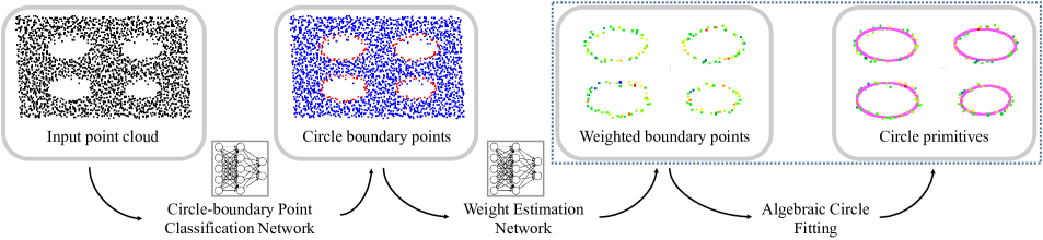
Figure 4: Overview of our point cloud circle algebraic fitting network: given a raw point cloud with multiple circles in it, we first extract all potential circle-boundary points by a point classification network. Then, we learn to estimate the weight of each circle-boundary point for serving algebraic circle fitting. By such a cascaded classification-and-fitting learning paradigm, circles in the point cloud can be learned effectively. Please note that the circle fitting step is embedded in the network.

2.3 Deep learning for unstructured point clouds

Since point clouds are unstructured and orderless, it is infeasible to directly apply standard CNNs. To resolve this problem, Qi et al (2017a) propose PointNet to learn per-point features using shared MLPs and global features using symmetrical pooling functions. Later, based on the PointNet, a series of point-based learning networks have been proposed (Jiang et al (2018); Engelmann et al (2018); Zhao et al (2019b); Zhang et al (2019); Hu et al (2020); Wang et al (2019); Zhao et al (2020); Wang et al (2021)).

Many networks are also elaborately designed for geometry extraction based on PointNet. For example, Wang et al (2020) introduce an end-to-end learnable technique, PIE-NET, to robustly identify feature edges in 3D point cloud data. Li et al (2019) propose a supervised geometric primitive fitting method that detects a varying number of primitives with different scales and design a differentiable primitive model estimator to solve a series of linear least-squares problems, which makes their whole network end-to-end trainable. Our method has three main differences: (1) Li et al (2019) use the PointNet++ to extract point-wise features, while our method employs the transformer module to obtain more effective deep features, which produces more accurate classification results. (2) In Li et al (2019), all points with their classification probabilities take part in the fitting process of all primitives. This kind of weighted fitting contributes more to classification, rather than as a fitting significance. We separately learn the circle boundary-point classification probabilities and fitting weights for only circle-boundary points. In our early experiments, we find that our schemes produce more accurate detection results and fitting results. (3) The approach in Li et al (2019) classifies points into instances during the learning process. So, it requires setting a fixed instance number. By contrast, we use a non-learning way, RANSAC, to cluster circle instances. This avoids pre-defining the number of instances in the input data. Angelina Uy et al (2021) propose differentiable algorithms suitable for a neural architecture, which partitions a point cloud into a set of Extrusion Cylinders. Sharma et al (2020) give an end-to-end differentiable approach for extracting an assembly of parametric primitives from a raw 3D point cloud. Paschalidou et al (2019) propose a learning-based approach for parsing 3D objects into consistent superquadric representations. Yu et al (2018) present an edge-aware network, EC-Net, to learn edges on point clouds using a deep architecture. Loizou et al (2020) propose a probabilistic boundaries detection approach based on a graph convolutional network to localize boundaries of semantic parts or geometric primitives. Different from above approaches, in this work, we present a new learning-based circle primitive method, by combining advanced point-based network and traditional algebraic methods, which makes our method more effective and explainable.

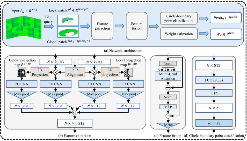
Figure 5: Detailed architecture of our Circle-Net. (a) is the full network architecture including both circle-boundary point classification and weight estimation. (b) to (d) are the feature extraction module, the feature fusion module and the circle-boundary point classification module in (a) respectively. The structure of the weight estimation module is similar to (d).

3 Overview

Motivation: Circle extraction from point clouds are divided to two (individual) operations: (1) classifying circle-boundary points; and (2) fitting a series of circles from these classified circle-boundary points. The first operation is sensitive to the quality of raw point clouds when determining whether each point in the point cloud is a circle-boundary point or not, and the second operation requires well-designed fitting or weighting functions when regressing circle parameters. The key idea of our framework is to combine learning-based local feature representation and traditional algebraic fitting model together, to robustly and accurately fit circles in the deep learning fashion.

We provide a brief overview of Circle-Net. It expects a raw point cloud $\mathbb{P}=\left\{\mathbf{p}_{i}\right\}_{i=1}^{N}\subset R^{3}$ as input, and aims at automatically detecting all potential circle-boundary points ${Q}_{f}$, while accurately computing circle parameters ($\mathbf{c}_{j}$, $r_{j}$) for each circle ($\mathbf{c}_{j}$ and $r_{j}$ are the circle center and radius, respectively). At the top level, Circle-Net consists of two cascaded sub-learning stages as shown in Fig. 4. Note that the weighted algebraic circle fitting step is embedded in the weight learning stage.

Circle-boundary Point Classification: We start by proposing a circle-boundary point classification network. First, we build two different neighborhoods and their corresponding 2D projection maps for each point, for perceiving multi-modality, multi-scale contextual information. The two neighborhoods contain a small local part of a circular structure, and a global patch covering an entire circle. Four different deep features of the two patches are then extracted by PointNet-like 3D networks and ResNet-like 2D networks, respectively. A transformer module is used to fuse the four features, for better distinguishing the points on the circle boundary and the points which are very close to the boundary. Finally, the fused features are exploited to regress the label of each point, i.e., the circle boundary or not.

Weight Estimation for Algebraic Circle Fitting: We leverage the learned features of circle-boundary points for robust circle fitting. A neural network is employed to estimate the weight of each detected circle-boundary point, which will be subsequently used for weighted algebraic circle fitting. The estimated weights can be intuitively interpreted as the significance metric for each point taking part in the traditional circle fitting operation. By such a soft selection mechanism, we can obtain more accurate circle parameters, than directly predicting these parameters.

4 Methodology

We start this section by first providing a simple background and mathematical notation for traditional circle fitting in Sec. 4.1. Then, in Sec. 4.2, we introduce how to use a network to detect circle-boundary points and how to synergize the learned deep features and traditional circle fitting. Sec. 4.3 describes our end-to-end joint loss function. Lastly, the multi-circle extraction strategy is introduced in Sec. 4.4.

4.1 Traditional Algebraic Circle Fitting Model

Traditional geometric approaches minimize the sum of the squared residuals:

$$\min\sum_{i=1}^{n}\left|r-\sqrt{(c_{x}-x_{i})^{2}+(c_{y}-y_{i})^{2}}\right|^{2}$$ (1)

where $(x_{i},y_{i})$ is the data point around a circle, $r$ is the circle radius, $(c_{x},c_{y})$ is the circle center. $|\cdot|$ denotes the absolute value function. Generally, the sampled points include noise and outliers, which could seriously reduce the accuracy of the fitting. To relieve it, the formulation given in Eq. 1 can be extended to a weighted version:

$$\min\sum_{i=1}^{n}(w_{i}\left|r-\sqrt{(c_{x}-x_{i})^{2}+(c_{y}-y_{i})^{2}}\right|)^{2}$$ (2)

where $w_{i}$ represents the weight of point $(x_{i},y_{i})$.

However, both Eq. 1 and Eq. 2 are non-linear least-squares problems, which have no closed-form solution and can only be solved by an iterative and expensive approach. An elegant alternative is to estimate the algebraic circle parameters:

$$A(x^{2}+y^{2})+Bx+Cy+D=0$$ (3)

where $A\neq 0$ and $B^{2}+C^{2}-4D>0$. The corresponding center $\mathbf{c}$ and radius $r$ are easily computed as:

$$c_{x}=-\frac{B}{2A},c_{y}=-\frac{C}{2A},r=\frac{\sqrt{B^{2}+C^{2}-4D}}{2A}$$ (4)

Then, we can minimize a parameter constrained approximation to Eq. 2:

$$\min\sum_{i=1}^{n}{w_{i}}^{2}(A(x_{i}^{2}+y_{i}^{2})+Bx_{i}+Cy_{i}+D)^{2}$$ (5)

Eq. 5 can be simply reformulated in the matrix form:

$$\min\mathbf{K}^{T}\mathbf{M}\mathbf{K}$$ (6)

where $\mathbf{K}=(A,B,C,D)$, $\mathbf{M}=\frac{1}{n}\mathbf{Z}^{T}\mathbf{W}^{T}\mathbf{W}\mathbf{Z}$, $\mathbf{Z}^{T}=\left[\mathbf{z}_{1},\mathbf{z}_{2},\ldots,\mathbf{z}_{n}\right]$, $\mathbf{z}_{i}=(x_{i}^{2}+y_{i}^{2},x_{i},y_{i},1)$, and $\mathbf{W}=diag(w_{i})$ is a diagonal matrix. $\mathbf{M}$ is a positive definite matrix. $\mathbf{H}$ is the constraint matrix which satisfies $\mathbf{K}^{T}\mathbf{H}\mathbf{K}=1$. We use the constraint matrix inspired by Hyper Al-Sharadqah et al (2009):

$$\mathbf{H}=\begin{bmatrix}8\sum w_{i}(x_{i}^{2}+y_{i}^{2})&4\sum w_{i}x_{i}&4\sum w_{i}y_{i}&2\\ 4\sum w_{i}x_{i}&1&0&0\\ 4\sum w_{i}y_{i}&0&1&0\\ 2&0&0&0\\ \end{bmatrix}$$ (7)

Eq. 6 can be solved as a generalized eigenvalue problem by using a Lagrange multiplier $\eta$. It then becomes an unconstrained minimization problem:

$$\min\mathbf{K}^{T}\mathbf{M}\mathbf{K}-\eta(\mathbf{K}^{T}\mathbf{H}\mathbf{K}-1)$$ (8)

Differentiating with respect to $\mathbf{K}$ and $\eta$, we obtain

$$\begin{array}[]{c}\mathbf{M}\mathbf{K}=\eta\mathbf{H}\mathbf{K}\\ \mathbf{K}^{T}\mathbf{H}\mathbf{K}=1\end{array}$$ (9)

Each solution ($\mathbf{K}$,$\eta$) of Eq. 9 can be obtain by calculating the generalized eigenvectors for the matrix pair $(\mathbf{M},\mathbf{H})$. The parameter $\mathbf{K}$ is the corresponding unit vector of the smallest positive $\eta$ from all the solutions. Then, the circle parameters can be calculated by Eq. 4.

4.2 Network Architecture

The architecture of our point cloud circle algebraic fitting network is illustrated in Fig. 5. Next, we would like to introduce the proposed network architecture in detail.

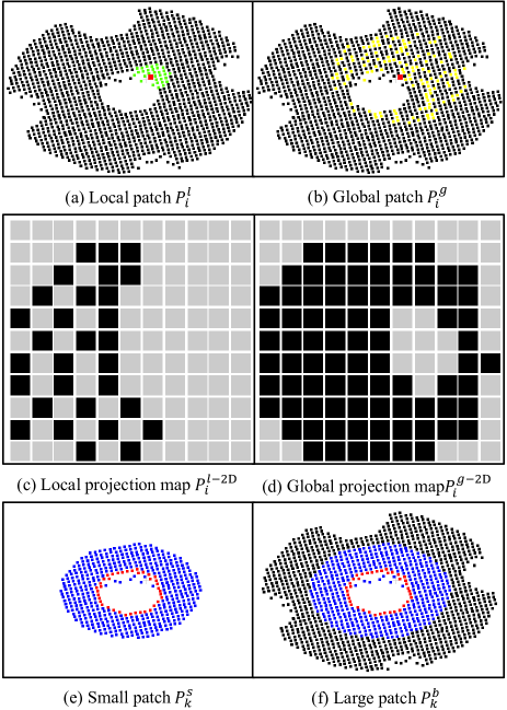
Figure 6: Illustration of the training data. The red point in (a) and (b) is the query point. The green points form the local patch, and the yellow points form the global patch. (c) and (d) are the 2D projection maps of the local and global patches in (a) and (b). (e) and (f) form a patch pair. (e) is the prepared point cloud to be classified, in which the red points are the circle-boundary points, and the blue points are the other points. (f) is a larger patch covering (a). During training, the local patch (a) and global patch (b) are extracted from (f) for each point in (e).

4.2.1 Circle-boundary point classification

Local/global patches generation. The key idea is to extract the potential boundary points only belonging to the circles, by fusing the multi-modality and multi-scale features, i.e., the local feature of circle boundary and the global feature of circle, the 3D feature of raw data and the 2D feature of projection map. This is because if only perceiving each point’s local context information, many near-circular boundary points may be misidentified as the circle-boundary points. Moreover, under the observation which a circular structure always locates on a planar-like surface, a 2D projection map is able to encode useful information of a circle structure. To this end, for each point in the small patch ${P}_{k}^{s}$ (Fig. 6 (e)), we use ball query search to build two neighborhoods and the corresponding 2D projection maps: the local patch $P_{i}^{l}$ (green points in Fig. 6 (a)), the global patch $P_{i}^{g}$ (yellow points in Fig. 6 (b)), the local projection map $P_{i}^{l-2D}$ (Fig. 6 (c)) and the global projection map $P_{i}^{g-2D}$ (Fig. 6 (d)). Note that we search neighboring points in the large patch ${P}_{k}^{b}$ with quarter and two times radius hyper-parameter $R^{hyper}$ (Fig. 6 (f)), respectively. To effectively tune network parameters with batch processing, the number of points in each input patch should be the same. We pad the origin for patches with insufficient points, and do random sampling for patches with sufficient points. The point numbers of local and global patches are fixed as $k_{l}=$ 16 and $k_{g}=$ 128 by trial and error.

Remark 1. To avoid the unnecessary degrees of freedom from feature space and make our network easier to train, we translate the center point to the origin. Besides, since a point cloud has no canonical orientation, and the point cloud with different poses should have the same detection results, we align the principle axis of $P_{i}^{l}$ and $P_{i}^{g}$ with the Z-axis by the transformation matrix formed by the principal axes of $P_{i}^{g}$. This is because that the global patch is more structure-aware, while the principal axes of the local patch are easier to be affected by the outliers. Then, all points of local patch and global patch are projected into the $11\times 11$ grids on the xy-plane separately. The values of grids with projection points are set to 1, and the others are 0. The values of all grids form two $11\times 11$ binary matrices as the inputs of projection maps.

Feature extraction. For each neighborhood and projection map, we extract its feature vector, by using 3D CNN and 2D CNN followed by a max-pooling operation. Both the 3D CNN and 2D CNN are composed of multi-layer perceptions (MLP). 3D CNN contains six layers: 64, 64, 128, 128, 256, 512, and 2D CNN contains four layers: 32, 128, 256, 512. In such a way, the feature from the local patch which captures local information, the feature from the global patch which is more shape-aware, and the feature from another type of modality, can be encoded simultaneously. The detailed feature learning module is shown in Fig. 5 (b).

Transformer-based feature fusion. As observed, the surrounding local structure of a circle-boundary point is very similar to that of its neighboring points. To further promote the accuracy of circle-boundary point classification, we exploit a transformer module to make full use of our extracted multi-modality and multi-scale features. In the feature fusion module, we feed the extracted four features to a Multi-Head Attention unit Dosovitskiy et al (2020), an MLP and an Average Pooling layer. Then, we get the integrated feature which fuses the boundary-level local information and the circle-level global information. Fig. 5 (c) shows the feature fusion module. Compared with the operation of direct feature concatenation, the transformer module is able to better capture the correlation between local and global information. Hence, the differences between the real circle-boundary points and their neighboring points will be easier to be perceived. Please refer to Sec. 6.3 for detailed qualitative and quantitative evaluation.

Circle-boundary point classification. In this step, a regressor (see from Fig. 5 (d)) is employed to evaluate the classification probabilities with the fused deep feature as input. The regressor is implemented by two fully connected layers and a softmax activation function which limits the classification probability to be within 0 and 1.

4.2.2 Weight estimation for circle fitting

The original data is noisy, and the extracted classification points may be also noisy. We improve the fitting effect by synergizing learning-based circle-boundary point feature representation and weighted algebraic fitting.

Weight learning. We borrow the fused feature from the feature fusion module and feed it to an MLP $h(\cdot)$, followed by a sigmoid activation function. We use the sigmoid to limit the output values within the range of 0 and 1. The output serves as a weight which measures the contribution of each point to the circle fitting task. Finally, we construct the diagonal weight matrix, $\mathbf{W}=diag(w_{i})$ with

$$w_{i}=\operatorname{sigmoid}\left(h\left(\mathbf{z}_{f}\right)\right)+\epsilon$$ (10)

where $\mathbf{z}_{f}$ is the fused feature. For the numerical stability, we add a constant small $\epsilon$ to avoid the degenerate case of a zero or poorly conditioned matrix. This weight matrix is then used to solve the circle fitting problem of Eq. 6.

4.3 Joint loss

Circle-Net is a cascaded classification-and-fitting circle extraction network. Its joint loss should cover two parts, i.e., the circle-boundary point classification loss and the fitting loss. Therefore, we formulate the joint loss function $L$ as the sum of the following two terms:

$$L=(1-\eta)*L_{c}+\eta*L_{f}$$ (11)

where $L_{c}$ is the circle-boundary point classification loss, and $L_{f}$ is the circle parameter learning loss. $\eta$ is a trade-off factor to balance the two terms (we empirically set $\eta=0.8$).

Circle-boundary point classification loss. The proportion of circle-boundary points in a point cloud is relatively low. We hence use the weighted cross-entropy loss to balance them:

$$\begin{split}L_{c}=\frac{1}{N}\sum_{i=1}^{N}w_{0}*(1-p_{i}^{label})*\log(1-p_{i}^{prob})+\\ w_{1}*p_{i}^{label}*\log(p_{i}^{prob})\end{split}$$ (12)

where $w_{0}$ and $w_{1}$ are category weights, which are determined by the number of samples. $N$ is the point number of the point clouds. $p_{i}^{label}$ is the point label (0 or 1). $p_{i}^{prob}$ is the predicted probability.

Fitting loss. The fitting loss function is formulated as the differences between $K$ fitted circle parameters ($\mathbf{c}_{j}$, $r_{j}$) and the corresponding ground truths ($\mathbf{\hat{c}}_{j}$, $\hat{r}_{j}$):

$$L_{f}=\frac{1}{K}\sum_{j=1}^{K}(r_{j}-\hat{r}_{j})_{2}^{2}+\left\|\mathbf{c}_{j}-\mathbf{\hat{c}}_{j}\right\|_{2}^{2}$$ (13)

4.4 Multi-circle fitting

Steps taken so far make it successful for us to obtain accurate individual circle primitives. Note that our goal is to extract all circle primitives, since an object may contain multiple circular structures. Instead of utilizing a network to learn all circle instances, during the test time, we use the RANSAC algorithm to cluster the points belonging to each circle, based on the results of circle-boundary point classification. There are two main reasons: i) for most objects, it is seldom to see two circles overlapping each other, and hence it is easy to segment them via the geometric technique; ii) the instance-level circle primitive learning from a raw scan is rather hard, without knowing some priors, such as circle numbers in this point cloud. Although we do not implement instance-level learning, when the input contains multiple circular structures, our method is still able to predict the label and the weight of each point. This makes the multi-circle fitting task very simple and feasible.

5 Training Data Preparation

Training dataset. In order to extract the potential circle-boundary points from raw data, it is necessary to add a label for each point for training. However, it is difficult to manually add labels in the noisy raw data acquired by a real scanner. As a result, we utilize a simulated scanner, which is developed by Blender, to virtually scan CAD models to generate raw data with different noise intensities and different resolutions, which are controlled by the parameters of the simulation software. In addition, circular structures in CAD models have different depths and we scan them from different views. Through the above schemes, we can obtain virtual point cloud data similar to the real-scanned. Notably, if we feed the complete point cloud into the network, we need to prepare many complete point clouds for training and the network will consume too many memories for neighbors searching. Hence, we crop patch pairs as input of our network, although we present a whole point cloud in Fig. 5.

Specifically, we use thirty CAD models, including curved and flat thin-walled planes with multiple circular structures. These circles have different radii, where the largest radius is about five times the smallest. The depth of each circular structure is between one-tenth and four times its radius. The angles between the scanned surface and the scanner are within fifteen and ninety degrees. Three different levels of noise (Gaussian noise with the standard deviation of 0.1%, 0.5%, and 1.0%) are added when virtually scanning each model. We also set three different sampling resolutions, to mimic more general scanning scenarios.

Before cropping patch pairs, we first calculate the ground-truth radii and centers of the scanned circular structures from CAD models. The computed radius and center of $j$-th circle are denoted as $\mathbf{\hat{c}}_{j}$ and $\hat{r}_{j}$. The radius of the largest circle is used as the radius hyper-parameter $R^{hyper}$. Next, forty patch pairs are extracted from each point cloud as the training data. Each patch pair $\langle{P}_{k}^{s},{P}_{k}^{b}\rangle$ contains a small point cloud patch ${P}_{k}^{s}$ (Fig. 6 (e)) and a large point cloud patch ${P}_{k}^{b}$ (Fig. 6 (f)). We construct each patch pair by ball query. The query radii for ${P}_{k}^{s}$ and ${P}_{k}^{b}$ are three and five times $R^{hyper}$, respectively, which are set empirically. ${P}_{k}^{s}$ is sufficiently large to contain any whole circular structure. ${P}_{k}^{b}$ is large enough to provide the complete neighborhood when each point in ${P}_{k}^{s}$ searches its neighborhood in ${P}_{k}^{b}$ during training. The query points include all circle centers and some randomly-sampled points. For each randomly-sampled point, its distance to any $\mathbf{\hat{c}}_{j}$ is either longer than $3\times R^{hyper}+\hat{r}_{j}$ or shorter than $3\times R^{hyper}$. Under the distance constraint, we keep that each ${P}_{k}^{s}$ either does not contain any part of circular structures, or contains circular structures larger than a semicircle. The goal for this design is to avoid detecting extremely incomplete circles. Totally, we create $30\times 3\times 3\times 40=12,000$ point cloud patch pairs for training. Tab. 1 concludes the training data enhancement operations.

Ground truth generation. We extract the ground-truth circle primitives directly from CAD models because our virtually scanned data is consistent with the corresponding CAD models. The ground truths contain two parts: labels of all points and parameters ($\mathbf{\hat{c}}_{j}$, $\hat{r}_{j}$) of all circles. We label all the virtually-scanned points into two categories: circle-boundary point set ${Q}_{f}$ and non-circle point set ${Q}_{nf}$. The points in ${Q}_{f}$ are edge points or boundary points of the circles in the raw point clouds (red points in Fig. 6 (e) and (f)). Non-circle points in ${Q}_{nf}$ lie in the other surface regions (blue and black point in Fig. 6 (e) and (f)). Detailedly, we label those points whose Euclidean distance to the noiseless high-density point set ${Q}_{gt}$ is less than a threshold as the circle-boundary points, and the others as non-circle boundary points:

$$\begin{array}[]{l}{Q}_{f}=\left\{\mathbf{p}_{i}\in\mathbb{P}\mid\left\|\mathbf{p}_{i}-\mathbf{q}_{gt}\right\|_{2}<t,\exists\mathbf{q}_{gt}\in{Q}_{gt}\right\}\\ {Q}_{nf}=\left\{\mathbf{p}_{i}\in\mathbb{P}\mid\left\|\mathbf{p}_{i}-\mathbf{q}_{gt}\right\|_{2}\geq t,\forall\mathbf{q}_{gt}\in{Q}_{gt}\right\}\end{array}$$ (14)

where ${Q}_{gt}$ is the accurate circle-boundary point set, and it is sampled from ground-truth circle curves, which are extracted by a CAD software. $t$ is a threshold which is set as the average neighboring point distance in $\mathbb{P}$. $\|\cdot\|_{2}$ denotes the $l_{2}$-norm. Notably, the accurate circle parameters ($\mathbf{\hat{c}}_{j}$, $\hat{r}_{j}$) are also directly generated by CAD software.

During the test, our method is capable of detecting circular structures with different radii, since our training data contains circles with different radii. When dealing with some circles, whose radii are very different from the training data, we need to adjust the radius hyper-parameter $R^{hyper}$. Its value is approximately set as the target circle radius.

Table 1: Data enhancement of training data.

Description	Operation
Shape	Thirty multi-circle CAD models, including both curved and flat thin-walled planes
Radius	The largest radius is about five times the smallest
Depth	Between one-tenth and four times the radius
Scanning direction	Between fifteen and ninety degrees
Noise	0.1%, 0.5%, and 1.0% Gaussian noise
Density	Three different sampling resolutions

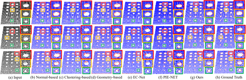
Figure 7: Comparison of the circle boundary detection results on virtually-scanned point clouds. The input in each row contains 18 circular structures with 6 different radii. The noise level of each row is 0.1%, 0.5% and 1%, respectively. The zoomed regions highlight the fact that our approach achieves better detection results, compared to previous techniques.

Table 2: Quantitative result of the circle boundary detection accuracy comparisons on the virtually-scanned data from normal-based Rusu and Cousins (2011), cluster-based Gersho and Gray (2012), geometry-based Belton and Lichti (2006), EC-Net Yu et al (2018), PIE-NET Wang et al (2020), and our classification network ($Precision-\%,Recall-\%,F1-\%$).

Method	Normal-based	Clustering-based	Geometry-based	EC-NET	PIE-NET	Ours
$Precision$	39.04	40.38	33.93	32.60	77.95	86.06
$Recall$	70.10	22.15	69.81	26.82	69.79	77.62
$F1$	49.21	28.61	45.66	29.43	73.64	81.58

Table 3: Quantitative evaluation of the circle fitting results on testing dataset shows the fitting error comparisons on weighted circle-boundary points from Hyper Al-Sharadqah et al (2009), LLS Coope (1993), RANSAC Fischler and Bolles (1981), RLTS Nurunnabi et al (2018), PIE-NET Wang et al (2020) and our method, including average center deviation ($AD(\mathbf{c})-mm$), average radius deviation ($AD(r)-mm$) and mean squared error of radius ($MSE(r)-mm^{2}$). The best results are in bold.

Noise level	0.1% noise			0.5% noise			1% noise
Method	$AD(\mathbf{c})$	$AD(r)$	$MSE(r)$	$AD(\mathbf{c})$	$AD(r)$	$MSE(r)$	$AD(\mathbf{c})$	$AD(r)$	$MSE(r)$
Hyper	0.465328	0.296654	0.089543	0.38116	0.31696	0.103115	0.667738	0.271244	0.076074
LLS	0.466897	0.296752	0.089596	0.385131	0.321495	0.105989	0.675546	0.279059	0.08018
RANSAC	0.438734	0.309176	0.103949	0.454232	0.377379	0.172154	0.809487	0.281098	0.108321
RLTS	0.469162	0.278478	0.080783	0.50883	0.239431	0.092588	0.707097	0.252474	0.075499
PIE-NET	0.649781	0.312905	0.121466	0.67379	0.312294	0.155506	0.783924	0.268966	0.207283
Ours	0.421035	0.103621	0.016823	0.398301	0.082654	0.01207	0.671365	0.016359	0.006351

6 Results and Discussion

In this section, to verify the effectiveness of the proposed method, we experiment with our method on a variety of virtually-scanned and real-scanned point clouds. Specifically, we compare our circle-boundary point classification scheme with several classical boundary detection methods, including the normal-based method Rusu and Cousins (2011) (implemented in the point cloud library, i.e., PCL), the clustering-based method Gersho and Gray (2012), the geometry-based method Belton and Lichti (2006), and the learning-based methods (EC-Net Yu et al (2018) and PIE-NET Wang et al (2020)). For the circle fitting part, we use the circle-boundary points classified by our method as the input, and then compare our fitting results with those produced by other approaches, including Hyper Al-Sharadqah et al (2009), LLS Coope (1993), RANSAC Fischler and Bolles (1981), RLTS Nurunnabi et al (2018) and PIE-NET Wang et al (2020). All the results of compared methods are produced by their released codes or with the help of the open source library, like PCL Rusu and Cousins (2011). For fair comparisons, the parameters of each method are tuned carefully, based on the recommended values. Besides, to make a fairer comparison with PIE-NET, we remove its corner point classification branch, open curve branch, and the corresponding loss, and encourage it to focus only on circle detection. Then, we train it on our patch-pair training data.

Notably, a circle is a 2D structure. When we draw it, we need to know a projection plane, which is determined by a normal direction and a point on this plane. For all the methods, the plane points are their own fitted circle centers. One evident difference is that our method computes the normal direction by weighted PCA, and the weights used are produced by the proposed network, while for the compared methods, the plane normal is computed by PCA.

6.1 Comparison of circle boundary detection

We test the six algorithms of boundary detection using 54 virtually-scanned point clouds with a total of 286K points. The circular structures have different radii. An example with 18 circles is shown in Fig. 7. The inputs are corrupted by 0.1%, 0.5% and 1% Gaussian noise, respectively. Note that these circular structures in CAD models are parts of cylinders formed when drilling holes. Those points from the surfaces of the cylinder, which are also close to the circle boundary, increase the difficulty of boundary detection.

Subjective evaluation. From the results in Fig. 7, only our algorithm successfully detects circle-boundary points. For the other five methods, this task is quite challenging. The reason is that the boundary points of a circular structure include edge points and open boundary points, and the five compared methods cannot distinguish that the open boundary points are located on the circles or the other structures. Moreover, due to not knowing where an accurate circle border is, the other methods can only roughly detect the boundary point set, which may contain those points very close to the circle boundaries. In contrast, our algorithm can well detect accurate circle-boundary points, by learning from the training data labeled with ground truths.

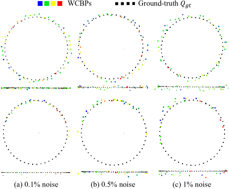
Figure 8: Visualization of the learned weights. There are six circles with three different-level noise. The circles in the first row are complete, and the circles in the bottom row are semi-circles. Red and blue colors represent the highest weight and the lowest weight, respectively, and the black points are ground-truth points of each circle. It is obvious to see that the boundary points near the black circle are almost red or yellow, which means they have higher weight. The results of color distribution prove that our weight learning module works well.

Objective evaluation. Apart from the visual results, the quantitative evaluation on the 54 virtually-scanned point clouds is reported in Tab. 2. $Precision$, $Recall$, and $F1$ are the three metrics:

$$\begin{array}[]{c}Precision=\frac{\#\text{ correctly detected circle-boundary points }}{\#\text{ all detected circle-boundary points }}\times 100\%\\ \\ Recall=\frac{\#\text{ correctly detected circle-boundary points }}{\#\text{ all ground-truth circle-boundary points }}\times 100\%\\ \\ F1=\frac{2Precision\times Recall}{Precision+Recall}\times 100\%\end{array}$$ (15)

Tab. 2 shows the detection accuracy results. Obviously, our method has the best results on both three metrics.

6.2 Comparison of circle fitting

To verify the effectiveness of the learning-based circle fitting, we first visualize the weight learning results, and then evaluate the accuracy of the fitted circle results.

Weight visualization. Since one of the main contributions of this work is to set the fitting weights in a data-driven way, we visualize the learned weights on three complete-circle points and three semi-circle points with different-level noise, as shown in Fig. 8. The black points are the precise circle-boundary points, and the other colorful points are the learned circle-boundary points, which are colorized by their corresponding weights. We call them weighted circle-boundary points (WCBPs). The redder the color, the greater the weight. It can be found that the yellow and red points are closer to the ground-truth circle, and the points far away from the ground-truth circle tend to be green and blue. Besides, even if the input is very noisy and incomplete, our weight learning module still yields reliable weights for circle fitting. This observation is consistent with our intuition.

Table 4: Quantitative comparison of circle boundary detection for different network variants ($Precision-\%,Recall-\%,F1-\%$). The last column $"Full"$ denotes our full pipeline.

Method	$Precision$	$Recall$	$F1$
$Variant\_1$	80.47	71.08	75.49
$Variant\_2$	84.45	76.91	80.51
$Variant\_3$	78.75	72.55	75.52
$Variant\_4$	79.40	74.37	76.80
$Variant\_5$	83.18	75.95	79.40
$Full$	86.03	77.62	81.58

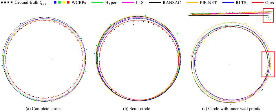
Figure 9: Circle fitting comparisons. We compare circle fitting with the other five methods by fitting the weighted circle-boundary points. (a) to (c) are the comparison results of a complete circle, semi-circle and circle with inner-wall points (in the red box). It can be seen from each result that the circle fitted by our method is closest to the ground truth.

Table 5: Quantitative comparison of circle fitting results of different network variants ($AD(\mathbf{c})-mm,AD(r)-mm,MSE(r)-mm^{2}$).

Noise level	0.1% noise			0.5% noise			1% noise
Method	$AD(\mathbf{c})$	$AD(r)$	$MSE(r)$	$AD(\mathbf{c})$	$AD(r)$	$MSE(r)$	$AD(\mathbf{c})$	$AD(r)$	$MSE(r)$
$Variant\_1$	0.47372	0.291626	0.086550	0.378543	0.284565	0.083755	0.683557	0.203256	0.043517
$Variant\_2$	0.441876	0.313686	0.100596	0.361986	0.330956	0.111946	0.668966	0.277501	0.079145
$Variant\_3$	0.502384	0.283151	0.082876	0.484761	0.219477	0.069472	0.910986	0.022152	0.103095
$Variant\_4$	0.448136	0.266749	0.083464	0.364695	0.235270	0.073410	0.691933	0.086769	0.033559
$Variant\_5$	0.432098	0.127128	0.018671	0.42052	0.093475	0.01345	0.680641	0.018848	0.007759
$Full$	0.421035	0.103621	0.016823	0.398301	0.082654	0.01207	0.671365	0.016359	0.006351

Accuracy of circle fitting. We compare the circle primitive extraction results of five methods. Fig. 9 demonstrates the visual fitting results. Three circle-boundary point inputs in Fig. 9 are complete, semi-complete, and polluted by strong outliers, respectively. They are the circle boundary detection results of our method. Each circle is an instance of the 54 virtually-scanned point clouds. Note that PIE-NET uses its own circle boundary detection results. It can be seen that the results of our method are closest to the ground-truth circles. There are two main reasons: i) the identified circle-boundary point set inevitably contains erroneous points; ii) when using a 3D scanner to reconstruct a circular structure, the acquired points do not exactly locate on the circle boundary. Also, we cannot define where the accurate circle boundary position is from discrete real-scanned point clouds, in nature. This is an ill-posed problem. Those robust fitting methods design various weighting functions to strengthen the robustness to the incorrect points (e.g., some outliers). However, their results always exist certain deviations to the accurate boundary. Unlike these methods, our approach is under the supervision of ground truths. By such a learning process, our method can infer more reliable circle parameters, from discrete circle-boundary points.

In addition to the above visual comparisons, we also objectively evaluate the performance of our learning-based circle fitting algorithm and compare it with other fitting methods. The inputs are the circle-boundary point classification results of our method on the fifty-four virtually-scanned point clouds. PIE-NET uses it own circle boundary detection results. For evaluating the accuracy of estimated circles, we compute the average center deviation $AD(\mathbf{c})$ between the estimated centers and the precise centers, the average radius deviation $AD(r)$, and the mean squared error of radius $MSE(r)$:

$$\begin{array}[]{c}AD(\mathbf{c})=\frac{1}{K}\sum_{j=1}^{K}\left\|\mathbf{c}_{j}-\hat{\mathbf{c}_{j}}\right\|_{2}\\ \\ AD(r)=\frac{1}{K}\sum_{j=1}^{K}|r_{j}-\hat{r}_{j}|\\ \\ MSE(r)=\frac{1}{K}\sum_{j=1}^{K}\left(r_{j}-\hat{r}_{j}\right)^{2}\end{array}$$ (16)

where $\mathbf{c}_{j}$ is the estimated circle center, $\hat{\mathbf{c}_{j}}$ is the accurate circle center, $r_{j}$ is the estimated circle radius, $\hat{r}_{j}$ is the accurate radius, and $K$ is the number of circles. From Tab. 3, it can be seen that our method achieves the lowest $AD(\mathbf{c})$ and $AD(r)$ among the five compared fitting approaches on the testing dataset. The quantitative comparison results further demonstrate the superiority of our learning-based weighted fitting over the other competing approaches.

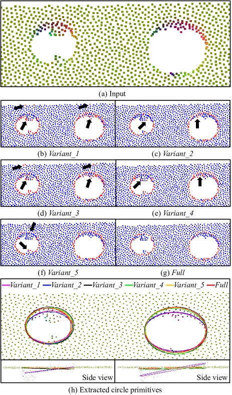
Figure 10: Comparison of ablation learning results. (a) is a real-scanned input data with two circles (scanned by a PhoXi 3D Scanner S). (h) is the extracted circle primitives of all network variants. From (b) to (g): the circle boundary detection results by different network variants. Black arrows indicate some unpleasing recognition results.

6.3 Ablation analysis

In this section, we take ablation experiments to analyze the contributions of the major modules in our method, by designing several variants of our method, as follows:

$\bullet\ Variant\_1$: replacing the transformer module with contacting the features of local patch and global patch directly, and fitting circles without the learning weights, namely, all the weights are set to 1.

$\bullet\ Variant\_2$: using the transformer module to fuse the features of local patch and global patch, and fitting circles without the learning weight. All the weights are set to 1.

$\bullet\ Variant\_3$: replacing the transformer module with concatenating the features of local patch and global patch directly, and fitting circles with the learning weights.

$\bullet\ Variant\_4$: replacing the transformer module with the attention module in Hu et al (2018) to fuse the features of local patch and global patch, and fitting circles with the learning weights.

$\bullet\ Variant\_5$: using the transformer module to fuse the features of local patch and global patch, and fitting circles with the learning weights.

$\bullet\ Full$: using the transformer module to fuse the the features of local patch, global patch, local projection map and global projection map, and fitting circles with the learning weights.

We retrain the five variants, and give visual comparisons in Fig. 10, followed by the quantitative evaluation of circle boundary detection and circle fitting in Tab. 4 and Tab. 5.

The input of Fig. 10 is a real-scanned point cloud that contains two circles with different sizes. The inputs of Tab. 4 are the fifty-four virtually-scanned point clouds. In Fig. 10, $Variant$_$2$ and $Variant$_$5$ have better circle-boundary point classification results than $Variant$_$1$ and $Variant$_$3$, and $Full$ is better than $Variant$_$5$ without mistaking other kinds of boundary points (see the black arrows). The quantitative results in Tab. 4 also prove them. It can be seen that the transformer module improves the $Precision$ of $Variant$_$2$ and $Variant$_$5$ by 3.98% and 4.43%, the $Recall$ by 5.83% and 3.4%, and the $F1$ by 5.02% and 3.88%, respectively. The 2D projection module improves the three metrics of $Full$ by 2.86%, 1.67% and 2.18%. These results prove that the transformer module and 2D projection module can increase the accuracy of circle boundary detection. They reduce the boundary points that do not belong to any circular structure and well distinguish the non-boundary points that are adjacent to the circle boundary points. The reason is that the transformer module can better capture the correlation between multi-modality and multi-scale features to determine whether a boundary point belongs to a circular structure. Besides, they can perceive the differences between the circle-boundary points’ features and their adjacent points’ features. By comparing the circle boundary detection results of $Variant$_$3$, $Variant$_$4$ and $Variant$_$5$, the attention module in $Variant$_$4$ improves the $Precision$ by 0.65%, the $Recall$ by 1.92%, and the $F1$ by 1.28%, respectively. However, its effect is worse than the transformer module. This is because the transformer module can fuse features better than the general attention module.

The fitted circle primitives are shown in Fig. 10 (h). It can be found that, by using the weight learning module, all the fitting results of $Variant$_$3$, $Variant$_$4$, $Variant$_$5$ and $Full$ are more immune to the outliers. The quantitative evaluation of circle fitting is shown in Tab. 5. The inputs of each variant are its own circle boundary detection results achieved on the fifty-four virtually-scanned point clouds. Our weight learning module produces more accurate circle primitives. Moreover, comparing the fitting results of $Variant$_$3$, $Variant$_$5$, and $Full$, the transformer module and 2D projection module can improve the fitting accuracy effectively. Note that we have also tried to directly regress the circle parameters, without incorporating the weighted circle fitting method. However, the learned result is very undesirable. The radius error is nearly 0.5 $mm$. The reason is that the combination of learning-based feature representation and traditional fitting model makes the learning process easier and more interpretable, than directly learning the parameters of circles.

6.4 More results on raw point clouds

The above experiments have proved that our method is effective on the virtually-scanned data. In addition, we also test the generalization ability on 10 real-scanned point clouds, as shown in Fig. 11. Our algorithm successfully detects most of the circle-boundary points. However, our method may also misidentify some boundary points of the circle-like structure (third row in Fig. 11) and some noisy points (fifth row in Fig. 11). Moreover, Fig. 12 shows the circle fitting result of a car engine with very complex structures. This raw input contains multi-scale circles, large missing regions, and noise. Note that we use the region growing algorithm to segment this input into small smooth parts before testing it. Although there are still some errors in the circle boundary detection result, our method is robust to the erroneous points and successfully fits the circles in the car engine data.

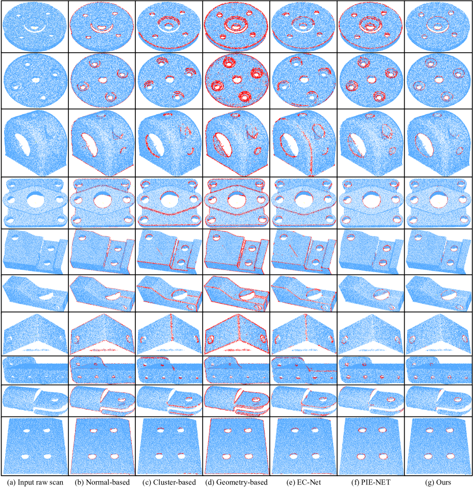
Figure 11: Comparison of circle boundary detection results on 10 real-scanned point clouds (scanned by MetraSCAN 3D Scanner). The results show that our approach achieves better detection results, compared to previous techniques.

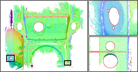
Figure 12: Circle fitting results on a real-scanned car engine point cloud with multiple circular structures (acquired by MetraSCAN 3D Scanner).

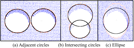
Figure 13: Results of two adjacent circles, two intersecting circles and an ellipse on the virtually-scanned data.The red points are the detected circle-boundary points and the black lines are the fitted circles

6.5 Effectiveness on some special cases

To demonstrate the effectiveness of our method in some special cases, Fig. 13 (a), (b), and (c) show the results of our method on two adjacent circles, two intersecting circles, and an ellipse structure, respectively. It can be seen that our method successfully detects the adjacent circles and the intersecting circles. However, in the result of the ellipse data, our method extracts the circle-boundary points but fits them into a circle rather than an ellipse.

6.6 Implementation

We implement the networks with Pytorch and train them on an NVIDIA Geforce GTX 1080 GPU. The network is trained with the Adam Optimizer, by a learning rate of 0.00001 for 400 epochs. The accuracy for the training dataset and test dataset and the loss for the training dataset are shown in Fig. 14.

Timing. Generally, the training takes about 8 hours. During testing, we conduct all experimental cases on a desktop PC with a 3.4 GHz Intel Core i7 CPU and 16 GB of RAM. Our method consumes around 5 seconds on a virtually scanned point cloud with 53000 points and 18 circles.

6.7 Application

Based on the proposed circle-boundary point classification and weighted algebraic circle fitting algorithms for circle primitives extraction, we develop a practical application in the quality inspection of drilling, which achieves favorable results, in terms of accuracy. The quality of drilling is a vital factor affecting the riveting quality of aircraft. Good riveting can improve the stability of the connection, reduce vibration, and prolong the service life of aircraft.

We test our approach on fifteen standard drilling parts with different circle radii ranging from 2.501 $mm$ to 2.524 $mm$, as shown in Fig. 15 (a). These drilling parts are standard parts, and the holes are precisely machined, whose radius errors are all less than 0.001 $mm$. Thus, we can regard them as the ground truths of quantitative comparison. To verify the accuracy of our method, we first use a high-precision 3D laser scanner to obtain the real-scanned point clouds of these parts (Fig. 15 (b)). The circle-boundary points are computed by five competing methods (see from Fig. 15 (c) to (g) and our method (Fig. 15 (h)). It can be seen that the circle boundary detection results of our approach are the cleanest. In Tab. 6, we report the fitting errors. The inputs are the circle boundary detection results of our method on the real-scanned data of fifteen standard drilling parts, except that PIE-NET uses its own boundary detection results. Our method achieves the lowest error, even compared with the commercial inspection software, PolyWorks. Note that the fitting results of PolyWorks are yielded by an experienced engineer. Moreover, only our method meets the H accuracy requirement (0.02 $mm$) of standard rivet holes.

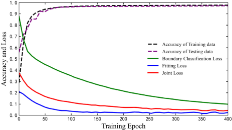
Figure 14: Accuracy for training dataset and test dataset and the loss for training dataset.

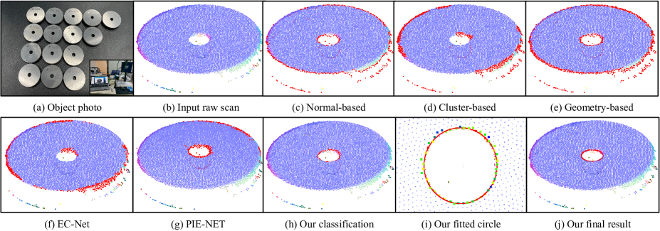
Figure 15: Visual results of rivet hole inspection on a real-scanned data (scanned by a Wenglor MLAS202 3D Scanner). (a) and (b) are the photo of a standard rivet hole and its corresponding real-scanned point cloud. From (c) to (h): The circle boundary detection results by normal-based Rusu and Cousins (2011), cluster-based Gersho and Gray (2012), geometry-based Belton and Lichti (2006), EC-Net Yu et al (2018), PIE-NET Wang et al (2020), and our classification network. (i) highlights a circle fitted with the learned point-wise weights. (j) is our circular structure inspection result. Our method can detect the circle primitive accurately.

Table 6: Quantitative evaluation of rivet hole inspection. The result shows the inspection error comparisons from Hyper Al-Sharadqah et al (2009), LLS Coope (1993), RANSAC Fischler and Bolles (1981), RLTS Nurunnabi et al (2018), PIE-NET Wang et al (2020), PolyWorks, and our method. PolyWorks is a commercial 3D inspection software ($AD(r)-mm,MSE(r)-mm^{2}$). As shown, our method achieves the best results.

Method	Hyper	LLS	RANSAC	RLTS	PIE-NET	PolyWorks	Ours
$AD(r)$	0.027201	0.028264	0.052397	0.068493	0.060182	0.0267	0.016884
$MSE(r)$	0.001113	0.001166	0.005844	0.009348	0.006742	0.001045	0.000530

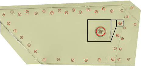
Figure 16: Circle fitting results on a real-scanned rivet point cloud with multiple circular structures (acquired by MetraSCAN 3D Scanner).

6.8 Experiments on outer circles

The circles detected above are all inner circles from drilling, but general circular structures also include outer circles, such as the edge of the cylinder. To detect the outer circles, we build the outer circle training set, and train our network on it. The test result on a real-scanned data is shown in Fig. 16. The detection object are the outer circles of rivets with a very low height, and the low-height circle is a difficulty in outer circle detection. As seen, our method succeeds in locating all the circle primitives automatically and accurately.

6.9 Limitation

Although our method can effectively extract circles from the real-scanned data, it still has some limitations.

$\bullet$ Our method may treat the ellipse or other circle-like shape as a circle. If we want to apply our method to correctly fit ellipses, we need to add ellipse data into the training set and revise the corresponding geometry fitting function.

$\bullet$ When dealing with some models with some circles whose size is very different with our training data, our method needs an approximate radius as the hyper-parameter $R^{hyper}$ during testing, for avoiding missing these circles.

7 Conclusion

We present a new method for multiple circle primitives learning from noisy yet incomplete point clouds. Taking a raw point cloud as input, our approach can accurately learn weighted circle-boundary points, which are further used for fitting circle primitives. Extensive experiments prove the effectiveness of our method and demonstrate its superiority in both circle boundary detection and circle fitting. The additional application further demonstrates the potential practical value in the field of 3D inspection.

Future work. It is our research interest to solve the traditional geometric optimization problem in a data-driven way, such as learning weights for geometric fitting. We plan to conquer the limitations of our method and extend this method to more geometry primitives in the future.

References

- Abdul-Rahman and Chernov (2014) Abdul-Rahman H, Chernov N (2014) Fast and numerically stable circle fit. Journal of mathematical imaging and vision 49(2):289–295
- Abelson et al (1985) Abelson H, Sussman GJ, Sussman J (1985) Structure and Interpretation of Computer Programs. MIT Press, Cambridge, Massachusetts
- Ahn et al (2001) Ahn SJ, Rauh W, Warnecke HJ (2001) Least-squares orthogonal distances fitting of circle, sphere, ellipse, hyperbola, and parabola. Pattern Recognition 34(12):2283–2303
- Akkiraju et al (1995) Akkiraju N, Edelsbrunner H, Facello M, Fu P, Mucke E, Varela C (1995) Alpha shapes: definition and softwaref. In: Proceedings of the 1st international computational geometry software workshop, vol 63, p 66
- Al-Sharadqah (2014) Al-Sharadqah A (2014) Further statistical analysis of circle fitting. Electronic Journal of Statistics 8(2):2741–2778
- Al-Sharadqah et al (2009) Al-Sharadqah A, Chernov N, et al (2009) Error analysis for circle fitting algorithms. Electronic Journal of Statistics 3:886–911
- Angelina Uy et al (2021) Angelina Uy M, Chang Yy, Sung M, Goel P, Lambourne J, Birdal T, Guibas L (2021) Point2cyl: Reverse engineering 3d objects from point clouds to extrusion cylinders. arXiv e-prints pp arXiv–2112
- Arandjelovic et al (2016) Arandjelovic R, Gronat P, Torii A, Pajdla T, Sivic J (2016) Netvlad: Cnn architecture for weakly supervised place recognition. In: Proceedings of the IEEE conference on computer vision and pattern recognition, pp 5297–5307
- Barber et al (1996) Barber CB, Dobkin DP, Huhdanpaa H (1996) The quickhull algorithm for convex hulls. ACM Transactions on Mathematical Software (TOMS) 22(4):469–483
- Baumgartner et al (2001) Baumgartner R, Gottlob G, Flesca S (2001) Visual information extraction with Lixto. In: Proceedings of the 27th International Conference on Very Large Databases, Morgan Kaufmann, Rome, Italy, pp 119–128
- Bazazian et al (2015) Bazazian D, Casas JR, Ruiz-Hidalgo J (2015) Fast and robust edge extraction in unorganized point clouds. In: 2015 international conference on digital image computing: techniques and applications (DICTA), IEEE, pp 1–8
- Belton and Lichti (2006) Belton D, Lichti DD (2006) Classification and segmentation of terrestrial laser scanner point clouds using local variance information. Int Arch Photogramm Remote Sens Spat Inf Sci 36(5):44–49
- Brachman and Schmolze (1985) Brachman RJ, Schmolze JG (1985) An overview of the KL-ONE knowledge representation system. Cognitive Science 9(2):171–216
- Calafiore (2002) Calafiore G (2002) Approximation of n-dimensional data using spherical and ellipsoidal primitives. IEEE Transactions on Systems, Man, and Cybernetics-Part A: Systems and Humans 32(2):269–278
- Chen et al (2021) Chen H, Huang Y, Xie Q, Liu Y, Zhang Y, Wei M, Wang J (2021) Multiscale feature line extraction from raw point clouds based on local surface variation and anisotropic contraction. IEEE Transactions on Automation Science and Engineering
- Chen et al (2019) Chen LZ, Li XY, Fan DP, Wang K, Lu SP, Cheng MM (2019) Lsanet: Feature learning on point sets by local spatial aware layer. arXiv preprint arXiv:190505442
- Chernov (2010) Chernov N (2010) Circular and linear regression: Fitting circles and lines by least squares. CRC Press
- Chernov and Lesort (2005) Chernov N, Lesort C (2005) Least squares fitting of circles. Journal of Mathematical Imaging and Vision 23(3):239–252
- Choi et al (2012) Choi C, Taguchi Y, Tuzel O, Liu MY, Ramalingam S (2012) Voting-based pose estimation for robotic assembly using a 3d sensor. In: 2012 IEEE International Conference on Robotics and Automation, IEEE, pp 1724–1731
- Cleveland (1979) Cleveland WS (1979) Robust locally weighted regression and smoothing scatterplots. Journal of the American statistical association 74(368):829–836
- Coope (1993) Coope ID (1993) Circle fitting by linear and nonlinear least squares. Journal of Optimization Theory and Applications 76(2):381–388
- De Guevara et al (2011) De Guevara IL, Muñoz J, De Cózar O, Blázquez EB (2011) Robust fitting of circle arcs. Journal of Mathematical Imaging and Vision 40(2):147–161
- De Marco et al (2015) De Marco T, Cazzato D, Leo M, Distante C (2015) Randomized circle detection with isophotes curvature analysis. Pattern Recognition 48(2):411–421
- Dorst (2014) Dorst L (2014) Total least squares fitting of k-spheres in n-d euclidean space using an (n+ 2)-d isometric representation. Journal of mathematical imaging and vision 50(3):214–234
- Dosovitskiy et al (2020) Dosovitskiy A, Beyer L, Kolesnikov A, Weissenborn D, Zhai X, Unterthiner T, Dehghani M, Minderer M, Heigold G, Gelly S, et al (2020) An image is worth 16x16 words: Transformers for image recognition at scale. arXiv preprint arXiv:201011929
- Duda and Hart (1972) Duda RO, Hart PE (1972) Use of the hough transformation to detect lines and curves in pictures. Communications of the ACM 15(1):11–15
- Engelmann et al (2018) Engelmann F, Kontogianni T, Schult J, Leibe B (2018) Know what your neighbors do: 3d semantic segmentation of point clouds. In: Proceedings of the European Conference on Computer Vision (ECCV) Workshops, pp 0–0
- Fan et al (2009) Fan H, Yu Y, Peng Q (2009) Robust feature-preserving mesh denoising based on consistent subneighborhoods. IEEE Transactions on Visualization and Computer Graphics 16(2):312–324
- Fischler and Bolles (1981) Fischler MA, Bolles RC (1981) Random sample consensus: a paradigm for model fitting with applications to image analysis and automated cartography. Communications of the ACM 24(6):381–395
- Frosio and Borghese (2008) Frosio I, Borghese NA (2008) Real-time accurate circle fitting with occlusions. Pattern Recognition 41(3):1041–1055
- Gersho and Gray (2012) Gersho A, Gray RM (2012) Vector quantization and signal compression, vol 159. Springer Science & Business Media
- Gottlob (1992) Gottlob G (1992) Complexity results for nonmonotonic logics. Journal of Logic and Computation 2(3):397–425
- Gottlob et al (2002) Gottlob G, Leone N, Scarcello F (2002) Hypertree decompositions and tractable queries. Journal of Computer and System Sciences 64(3):579–627
- Guo et al (2020) Guo MH, Cai JX, Liu ZN, Mu TJ, Martin RR, Hu SM (2020) Pct: Point cloud transformer. arXiv preprint arXiv:201209688
- Hu et al (2018) Hu J, Shen L, Sun G (2018) Squeeze-and-excitation networks. In: Proceedings of the IEEE conference on computer vision and pattern recognition, pp 7132–7141
- Hu et al (2020) Hu Q, Yang B, Xie L, Rosa S, Guo Y, Wang Z, Trigoni N, Markham A (2020) Randla-net: Efficient semantic segmentation of large-scale point clouds. In: Proceedings of the IEEE/CVF Conference on Computer Vision and Pattern Recognition, pp 11,108–11,117
- IJCAI Proceedings (????) IJCAI Proceedings (????) IJCAI camera ready submission. https://proceedings.ijcai.org/info
- Jiang et al (2018) Jiang M, Wu Y, Zhao T, Zhao Z, Lu C (2018) Pointsift: A sift-like network module for 3d point cloud semantic segmentation. arXiv preprint arXiv:180700652
- Kanatani and Rangarajan (2011) Kanatani K, Rangarajan P (2011) Hyper least squares fitting of circles and ellipses. Computational Statistics & Data Analysis 55(6):2197–2208
- Kanatani et al (2016) Kanatani K, Sugaya Y, Kanazawa Y (2016) Guide to 3D Vision Computation, vol 3. Springer
- Kåsa (1976) Kåsa I (1976) A circle fitting procedure and its error analysis. IEEE Transactions on instrumentation and measurement (1):8–14
- Kettner et al (2004) Kettner L, Näher S, Goodman JE, O’Rourke J (2004) Two computational geometry libraries: Leda and cgal. In: Handbook of Discrete and Computational Geometry, Chapman & Hall/CRC, pp 1435–1463
- Kleppe et al (2018) Kleppe AL, Tingelstad L, Egeland O (2018) Coarse alignment for model fitting of point clouds using a curvature-based descriptor. IEEE Transactions on Automation Science and Engineering 16(2):811–824
- Kleppe et al (2019) Kleppe AL, Tingelstad L, Egeland O (2019) Coarse alignment for model fitting of point clouds using a curvature-based descriptor. IEEE transactions on automation science and engineering 16(2):811–824
- Lafarge and Mallet (2012) Lafarge F, Mallet C (2012) Creating large-scale city models from 3d-point clouds: A robust approach with hybrid representation. International Journal of Computer Vision 99(1):69–85
- Levesque (1984a) Levesque HJ (1984a) Foundations of a functional approach to knowledge representation. Artificial Intelligence 23(2):155–212
- Levesque (1984b) Levesque HJ (1984b) A logic of implicit and explicit belief. In: Proceedings of the Fourth National Conference on Artificial Intelligence, American Association for Artificial Intelligence, Austin, Texas, pp 198–202
- Li et al (2010) Li B, Wang X, Yang H, Zhou Z (2010) Aircraft rivets defect recognition method based on magneto-optical images. In: 2010 International Conference on Machine Vision and Human-machine Interface, IEEE, pp 788–791
- Li et al (2019) Li L, Sung M, Dubrovina A, Yi L, Guibas LJ (2019) Supervised fitting of geometric primitives to 3d point clouds. In: Proceedings of the IEEE/CVF Conference on Computer Vision and Pattern Recognition, pp 2652–2660
- Loizou et al (2020) Loizou M, Averkiou M, Kalogerakis E (2020) Learning part boundaries from 3d point clouds. In: Computer Graphics Forum, Wiley Online Library, vol 39, pp 183–195
- Lu et al (2015) Lu X, Deng Z, Chen W (2015) A robust scheme for feature-preserving mesh denoising. IEEE transactions on visualization and computer graphics 22(3):1181–1194
- Lund (2013) Lund UJ (2013) Monte carlo maximum likelihood circle fitting using circular density functions. Computational Statistics 28(2):393–411
- Maligo and Lacroix (2016) Maligo A, Lacroix S (2016) Classification of outdoor 3d lidar data based on unsupervised gaussian mixture models. IEEE Transactions on Automation Science and Engineering 14(1):5–16
- Mineo et al (2019) Mineo C, Pierce SG, Summan R (2019) Novel algorithms for 3d surface point cloud boundary detection and edge reconstruction. Journal of Computational Design and Engineering 6(1):81–91
- Nebel (2000) Nebel B (2000) On the compilability and expressive power of propositional planning formalisms. Journal of Artificial Intelligence Research 12:271–315
- Nurunnabi et al (2014) Nurunnabi A, Belton D, West G (2014) Robust statistical approaches for local planar surface fitting in 3d laser scanning data. ISPRS journal of photogrammetry and Remote Sensing 96:106–122
- Nurunnabi et al (2015a) Nurunnabi A, West G, Belton D (2015a) Outlier detection and robust normal-curvature estimation in mobile laser scanning 3d point cloud data. Pattern Recognition 48(4):1404–1419
- Nurunnabi et al (2015b) Nurunnabi A, West G, Belton D (2015b) Robust locally weighted regression techniques for ground surface points filtering in mobile laser scanning three dimensional point cloud data. IEEE Transactions on Geoscience and Remote Sensing 54(4):2181–2193
- Nurunnabi et al (2018) Nurunnabi A, Sadahiro Y, Laefer DF (2018) Robust statistical approaches for circle fitting in laser scanning three-dimensional point cloud data. Pattern Recognition 81:417–431
- Öztireli et al (2009) Öztireli AC, Guennebaud G, Gross M (2009) Feature preserving point set surfaces based on non-linear kernel regression. In: Computer Graphics Forum, Wiley Online Library, vol 28, pp 493–501
- Paschalidou et al (2019) Paschalidou D, Ulusoy AO, Geiger A (2019) Superquadrics revisited: Learning 3d shape parsing beyond cuboids. In: Proceedings of the IEEE/CVF Conference on Computer Vision and Pattern Recognition, pp 10,344–10,353
- Pratt (1987) Pratt V (1987) Direct least-squares fitting of algebraic surfaces. ACM SIGGRAPH computer graphics 21(4):145–152
- Qi et al (2017a) Qi CR, Su H, Mo K, Guibas LJ (2017a) Pointnet: Deep learning on point sets for 3d classification and segmentation. In: Proceedings of the IEEE conference on computer vision and pattern recognition, pp 652–660
- Qi et al (2017b) Qi CR, Yi L, Su H, Guibas LJ (2017b) Pointnet++: Deep hierarchical feature learning on point sets in a metric space. arXiv preprint arXiv:170602413
- Rousseeuw (1984) Rousseeuw PJ (1984) Least median of squares regression. Journal of the American statistical association 79(388):871–880
- Rousseeuw and Leroy (2005) Rousseeuw PJ, Leroy AM (2005) Robust regression and outlier detection, vol 589. John wiley & sons
- Rusu and Cousins (2011) Rusu RB, Cousins S (2011) 3d is here: Point cloud library (pcl). In: 2011 IEEE international conference on robotics and automation, IEEE, pp 1–4
- Sharma et al (2020) Sharma G, Liu D, Maji S, Kalogerakis E, Chaudhuri S, Měch R (2020) Parsenet: A parametric surface fitting network for 3d point clouds. In: European Conference on Computer Vision, Springer, pp 261–276
- Taubin (1991) Taubin G (1991) Estimation of planar curves, surfaces, and nonplanar space curves defined by implicit equations with applications to edge and range image segmentation. IEEE Computer Architecture Letters 13(11):1115–1138
- Torr and Zisserman (2000) Torr PH, Zisserman A (2000) Mlesac: A new robust estimator with application to estimating image geometry. Computer vision and image understanding 78(1):138–156
- Wang and Suter (2003) Wang H, Suter D (2003) Using symmetry in robust model fitting. Pattern Recognition Letters 24(16):2953–2966
- Wang et al (2012) Wang J, Zhang X, Yu Z (2012) A cascaded approach for feature-preserving surface mesh denoising. Computer-Aided Design 44(7):597–610
- Wang et al (2020) Wang X, Xu Y, Xu K, Tagliasacchi A, Zhou B, Mahdavi-Amiri A, Zhang H (2020) Pie-net: Parametric inference of point cloud edges. arXiv preprint arXiv:200704883
- Wang et al (2019) Wang Y, Sun Y, Liu Z, Sarma SE, Bronstein MM, Solomon JM (2019) Dynamic graph cnn for learning on point clouds. Acm Transactions On Graphics (tog) 38(5):1–12
- Wang et al (2021) Wang Z, Xie Q, Lai YK, Wu J, Long K, Wang J (2021) Mlvsnet: Multi-level voting siamese network for 3d visual tracking. In: ICCV, pp 3101–3110
- Wei et al (2014) Wei M, Yu J, Pang WM, Wang J, Qin J, Liu L, Heng PA (2014) Bi-normal filtering for mesh denoising. IEEE transactions on visualization and computer graphics 21(1):43–55
- Wei et al (2016) Wei M, Liang L, Pang WM, Wang J, Li W, Wu H (2016) Tensor voting guided mesh denoising. IEEE Transactions on Automation Science and Engineering 14(2):931–945
- Xie et al (2020) Xie Q, Lu D, Du K, Xu J, Dai J, Chen H, Wang J (2020) Aircraft skin rivet detection based on 3d point cloud via multiple structures fitting. Computer-Aided Design 120:102,805
- Yang et al (2019) Yang J, Zhang Q, Ni B, Li L, Liu J, Zhou M, Tian Q (2019) Modeling point clouds with self-attention and gumbel subset sampling. In: Proceedings of the IEEE/CVF Conference on Computer Vision and Pattern Recognition, pp 3323–3332
- Yu et al (2018) Yu L, Li X, Fu CW, Cohen-Or D, Heng PA (2018) Ec-net: an edge-aware point set consolidation network. In: Proceedings of the European Conference on Computer Vision (ECCV), pp 386–402
- Zhang et al (2021) Zhang Q, Liu J, Zheng S, Yu C (2021) A novel accurate positioning method of reference hole for complex surface in aircraft assembly. The International Journal of Advanced Manufacturing Technology pp 1–16
- Zhang et al (2019) Zhang Z, Hua BS, Yeung SK (2019) Shellnet: Efficient point cloud convolutional neural networks using concentric shells statistics. In: Proceedings of the IEEE/CVF International Conference on Computer Vision, pp 1607–1616
- Zhao et al (2019a) Zhao C, Zhou W, Lu L, Zhao Q (2019a) Pooling scores of neighboring points for improved 3d point cloud segmentation. In: 2019 IEEE International Conference on Image Processing (ICIP), IEEE, pp 1475–1479
- Zhao et al (2019b) Zhao H, Jiang L, Fu CW, Jia J (2019b) Pointweb: Enhancing local neighborhood features for point cloud processing. In: Proceedings of the IEEE/CVF Conference on Computer Vision and Pattern Recognition, pp 5565–5573
- Zhao et al (2020) Zhao H, Jiang L, Jia J, Torr P, Koltun V (2020) Point transformer. arXiv preprint arXiv:201209164
- Zhao et al (2019c) Zhao W, Liu X, Wang S, Fan X, Zhao D (2019c) Graph-based feature-preserving mesh normal filtering. IEEE Transactions on Visualization and Computer Graphics
- Zhao et al (2019d) Zhao Y, Birdal T, Deng H, Tombari F (2019d) 3d point capsule networks. In: Proceedings of the IEEE/CVF Conference on Computer Vision and Pattern Recognition, pp 1009–1018
- Zheng et al (2017) Zheng Y, Li G, Wu S, Liu Y, Gao Y (2017) Guided point cloud denoising via sharp feature skeletons. The Visual Computer 33(6):857–867