Unbiased Top-$k$ Learning to Rank with
Causal Likelihood Decomposition

Abstract.

Unbiased learning to rank has been proposed to alleviate the biases in the search ranking, making it possible to train ranking models with user interaction data. In real applications, search engines are designed to display only the most relevant $k$ documents from the retrieved candidate set. The rest candidates are discarded. As a consequence, position bias and sample selection bias usually occur simultaneously. Existing unbiased learning to rank approaches either focus on one type of bias (e.g., position bias) or mitigate the position bias and sample selection bias with separate components, overlooking their associations. In this study, we first analyze the mechanisms and associations of position bias and sample selection bias from the viewpoint of a causal graph. Based on the analysis, we propose Causal Likelihood Decomposition (CLD), a unified approach to simultaneously mitigating these two biases in top-$k$ learning to rank. By decomposing the log-likelihood of the biased data as an unbiased term that only related to relevance, plus other terms related to biases, CLD successfully detaches the relevance from position bias and sample selection bias. An unbiased ranking model can be obtained from the unbiased term, via maximizing the whole likelihood. An extension to the pairwise neural ranking is also developed. Advantages of CLD include theoretical soundness and a unified framework for pointwise and pairwise unbiased top-$k$ learning to rank. Extensive experimental results verified that CLD, including its pairwise neural extension, outperformed the baselines by mitigating both the position bias and the sample selection bias. Empirical studies also showed that CLD is robust to the variation of bias severity and the click noise.

1. Introduction

In order to efficiently make use of user interaction data in learning of ranking models, studies on alleviating biases in user interaction data have been conducted, called Unbiased Learning to Rank (ULTR) (Ai et al., 2018; Hu et al., 2019; Ai et al., 2021) or Counterfactual Learning to Rank (CLTR) (Agarwal et al., 2019a; Jagerman et al., 2019; Oosterhuis and de Rijke, 2021b). Previously, studies focused on position bias and usually assumed that users can examine the whole ranking list so that every relevant document is guaranteed to be examined (Joachims et al., 2017; Carterette and Chandar, 2018; Craswell et al., 2008; Zhuang et al., 2021). Due to the limitation of the device sizes, however, search engines usually only display at most $k$ relevant documents to the user-issued query, on the basis of existing ranking models. It leads to the problem of unbiased top-$k$ learning to rank(Niu et al., 2012). If the ranking models are trained on the user interactions with these top-$k$ displayed documents, the sample selection bias will occur (Heckman, 1976, 1979). Moreover, the user interaction data gathered from the top-$k$ ranking positions still suffers from the effect of position bias, making unbiased top-$k$ learning to rank more challenging.

Recently, Oosterhuis and de Rijke (2020) developed policy-aware propensity scoring to eliminate sample selection bias. They prove that the policy-aware estimator is unbiased if every relevant item has a non-zero probability to appear in the top-$k$ ranking. However, to meet the critical assumption, the policy-aware estimator needs to know multiple logging policies and requires these policies to differ enough in their ranking results, which is actually a kind of expensive external intervention. Inspired by Heckman’s two-stage method (Heckman, 1979, 1976), Ovaisi et al. (2020) proposed Heckman^rank for top-$k$ learning to rank. In order to correct both the sample selection bias and position bias, RankAgg is proposed to combine the result of Heckman^rank and IPW (Inverse Propensity Weighting). Since position bias and sample selection bias were mitigated in two separated components and their associations were neglected, biased ranking results may still be generated. How to mitigate both position bias and sample selection bias simultaneously is still a challenging problem.

In this paper, we conducted an analysis on the effects of the biases compounded in user interactions, from the viewpoint of a causal graph. With the decomposition of the likelihood of top-$k$ ranking, we show that position bias is caused by the effect of examination in a different position and is a typical confounding bias. The sample selection bias, on the other hand, is actually a collider bias(Cole et al., 2010). Moreover, position bias and sample selection bias are associated in top-$k$ ranking. The click probability on a document is determined by both the displayed position and the selection of search engine. This indicates mitigating each bias separately can not lead to unbiased ranking results. The analysis also demonstrated that these two biases could be compounded in user interaction data, thus making the effect of bias even more severe. Mitigating one bias at a time won’t obtain an overall unbiased ranking result, motivating us to develop a new approach that can mitigate both two biases simultaneously.

Based on the analysis, we proposed a unified approach to mitigate the position bias and the sample selection bias simultaneously, called Causal Likelihood Decomposition (CLD). Unlike the existing studies that usually maximize the rewards for a ranking policy (Joachims and Swaminathan, 2016; Oosterhuis et al., 2020), CLD aims to maximize the log-likelihood of the observed user interaction data (Jeunen et al., 2020; Storkey, 2009). Specifically, CLD tries to decompose the log-likelihood function into an unbiased term that only related to the user-perceived relevance, plus other terms that related to the position bias or sample selection bias. In this way, the relevance signals are detached from the likelihood of observed user interaction data. Theoretical analysis showed that an unbiased relevance ranking model could be obtained from the unbiased term of the log-likelihood function when the whole log-likelihood is maximized. We also present an extension of the CLD in which the neural networks are adopted as the ranking model and selection model, and their parameters are learned with pairwise losses.

CLD offers several advantages: theoretical soundness, elegant extension to pairwise neural ranking, and high accuracy in unbiased top-$k$ learning to rank. The major contributions of this work are:

1. A theoretical analysis towards position bias and sample selection bias from the viewpoint of statistical causal inference;

2. A unified and theoretical sound approach to mitigating both position bias and sample selection bias in top-$k$ ranking. The method is derived under likelihood maximization and can be applied to both pointwise and pairwise training;

3. Extensive experiments on two publicly available datasets demonstrated the effectiveness of the proposed approaches over baselines for the task of unbiased top-$k$ learning to rank. The empirical analysis also showed the robustness of the approaches in terms of the variation of bias severity and the click noise.

2. Related work

2.1. Unbiased learning to rank

Recently, there has been a trend towards utilizing the user interaction data (e.g., the click log) as the substitute for the expert annotated relevance labels to train the ranking models in web search (Yuan et al., 2020; Hu et al., 2019; Wang et al., 2016). In contrast to the expert annotated labels, the user interaction data is massive, cheap, and most importantly, user-centric (Agarwal et al., 2019a). However, the behaviors of the users could probably be affected by some unexpected factors (Joachims et al., 2005), including the display ranking position (Joachims et al., 2007; Joachims et al., 2017; Ai et al., 2018; Agarwal et al., 2019c, a; Fang et al., 2019; Dong et al., 2020), the search engine’s selection (Ovaisi et al., 2020; Oosterhuis and de Rijke, 2020; Ovaisi et al., 2021), and others(Schnabel et al., 2016; Wang et al., 2019; Saito, 2020; Agarwal et al., 2019b; Vardasbi et al., 2020; Dong et al., 2020; Wei et al., 2021). These factors, along with users’ true perceived relevance, impact the observational user interaction data gathered from search engines. Although relevance signal is contained inside, the interaction data cannot be directly used to train the ranking models unless those aforementioned factors are eliminated. Otherwise, a biased ranking model would be learned and hurt the user experience (Chen et al., 2020).

To mitigate biases, unbiased learning to rank has attracted a lot of research efforts recently. Most approaches focus on addressing a single bias. For example, inverse propensity weighting (IPW) has been widely discussed in many studies (Joachims et al., 2017; Agarwal et al., 2019a) for addressing the position bias. It estimates the causal effect of examination and extracts them from the click signal directly. The top-$k$ cut-off of search engines leads to sample selection bias. Inspired by the famous Heckman’s two-stage method (Heckman, 1979, 1976), Ovaisi et al. (2020) proposed $Heckman^{rank}$ for top-$k$ learning to rank. Furthermore, Oosterhuis and de Rijke (2020) developed policy-aware propensity scoring to eliminate sample selection bias, by assuming that policy-aware estimator knows multiple differ enough logging policies.

In the real world, various biases could occur simultaneously (Chen et al., 2020). To address the trust bias and position bias simultaneously, Agarwal et al. (2019b) proposed a Bayes-IPS estimator. Affine-IPS (Vardasbi et al., 2020) improved Bayes-IPS and achieved better performance. Ovaisi et al. (2020) proposed RankAgg who ensembles the ranking results by the model for correcting position bias and the model for correcting sample selection bias. Ovaisi et al. (2021) proposed PIJD which does not require the exact propensity scores and can mitigate both position bias and sample selection bias. More recently, Oosterhuis and de Rijke (2021a) introduced an intervention-aware estimator for integrating counterfactual and online learning to rank, which can mitigate position bias, sample selection bias, and trust bias simultaneously. Chen et al. (2021) proposed AutoDebias that leverages the uniform data to learn the optimal debiasing strategy for various biases.

2.2. Causal inference in information retrieval

The generation of users’ implicit feedback in real search engines is affected by many biased factors. To make this feedback usable, causal inference has been introduced to analyze the generation procedure of users’ implicit feedback and mitigate bias inside. For instance, Zheng et al. (2021) analyzed the casual structure of popularity bias and proposed DICE to disentangle the user interest from click. Zhang et al. (2021) further analyzed the causal structure of item popularity and leveraged them to enhance the performance of recommendation. Wang et al. (2020) utilized the causal inference to handle the unobserved confounders in the recommendation.  Wang et al. (2021) proposed DecRs to dynamically regulate backdoor adjustment according to user status, thus eliminating the effect of confounders. However, few works conduct a systematical analysis for the bias in ranking from the viewpoint of causal inference.

3. Analyzing the Biases in top-k ranking

The problem of unbiased top-$k$ learning to rank can be described as follows. Given a user query $q$ and $K$ retrieved documents, each query-document pair $(q,d)$ is described by a feature vector $\mathbf{x}=\phi(q,d)\in\mathbb{R}^{n}$. The relevance of $(q,d)$ can be represented by an unobserved variable $R$, which could be binary, ordinal, or real. The retrieved documents are ranked by a logging policy (an existing ranking model) $\pi_{0}:\mathbb{R}^{n}\mapsto\{1,2,\cdots,K\}$ according to their features, where each document will be ranked at some position $P\in\{1,2,\cdots,K\}$ by $\pi_{0}$. In the real world, only the top $k\leq K$ documents can be presented to users due to some limitations (e.g., screen sizes). Let’s use $S\in\{0,1\}$ to denote whether a document is selected and presented to the user, i.e., $S=1$ if selected otherwise not. Further, let’s use $E\in\{0,1\}$ to denote that the user has examined the presented document, and $C\in\{0,1\}$ to denote whether a user clicks the document, which is a random variable obeying Bernoulli distribution(Joachims et al., 2017; Agarwal et al., 2019a; Vardasbi et al., 2020).

The user interactions with a search engine can be recorded as click log $\mathcal{D}=\{(\mathbf{x}_{i},c_{i},k_{i},s_{i})\}_{i=1}^{N}$, where $\mathbf{x}_{i},c_{i},k_{i},s_{i}$ respectively denote the $i$-th query-document pair’s feature vector, whether the document being clicked, the ranking position, and whether being selected. Ideally, we hope an unbiased ranking model could be estimated by maximizing the log-likelihood shown below:

(1) $$\begin{split}\mathcal{L}_{\mathrm{unbiased}}&=\sum_{i=1}^{N}\log\left(\mathrm{Pr}(r_{i}|\mathbf{x}_{i})\right),\end{split}$$

where the $r_{i}$ is the unobserved relevance for query-document pairs encoded by $\mathbf{x}_{i}$. Equation (1) cannot be maximized because $r_{i}$ cannot be observed directly.

On the other hand, we observed that the click log consists of two parts: $\mathcal{D}=\mathcal{D}_{s}\bigcup\mathcal{D}_{u}$, where $\mathcal{D}_{s}=\{(\mathbf{x}_{i},c_{i},k_{i},s_{i}=1)\}_{i=1}^{N_{s}}$ are the interactions for the $N_{s}$ selected $(q,d)$ pairs, and $\mathcal{D}_{u}=\{(\mathbf{x}_{i},c_{i}=0,k_{i},s_{i}=0)\}_{i=1}^{N_{u}}$ are those for the $N_{u}$ not selected pairs. A naive log-likelihood can be written as:

(2) $$\begin{split}\mathcal{L}_{\mathrm{naive}}&=\sum_{i=1}^{N_{s}}\log\left(\mathrm{Pr}(c_{i},s_{i}|\mathbf{x}_{i})\right)+\sum_{i=1}^{N_{u}}\log\left(\mathrm{Pr}(s_{i}|\mathbf{x}_{i})\right).\end{split}$$

Though it can be optimized, the naive log-likelihood suffers from both position bias from $c_{i}$ and the sample selection bias from $s_{i}$. There exists a large gap between the naive Equation (2) and the ideal unbiased objective Equation (1).

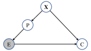
(a) Position bias

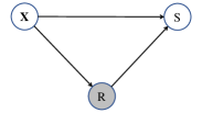
(b) Sample selection bias

Figure 1. The casual graphs of position bias (a) and sample selection bias (b). Each node corresponds a casual variable and the gray node means that the variable is unobserved.

Previous studies on the problem (Joachims et al., 2007; Joachims et al., 2017; Ai et al., 2018; Agarwal et al., 2019c, a; Fang et al., 2019) have made several assumptions. That is, for all $\mathbf{x}=\phi(q,d)$:

Assumption (1)::

The logging policy $\pi_{0}$ is deterministic, i.e., $d$ will always be displayed at a certain position $k$ by $\pi_{0}$:

$$\mathrm{Pr}(P=k|\mathbf{x})=\mathbbm{1}[k=\pi_{0}(\mathbf{x})];$$

Assumption (2)::

$d$ will not be clicked if it is not examined:

$$\mathrm{Pr}(C=1|E=0,\mathbf{x})=0;$$

Assumption (3)::

The click probability on $d$ is equal to its relevance $R(\mathbf{x})$ if and only if $d$ always be examined:

$$E\equiv 1\iff{\mathrm{Pr}(C=1|\mathbf{x})=R(\mathbf{x})}.$$

Note that Assumption (3) indicates the user’s click probability can represent a query-document’s relevance when it is always examined. This paper focuses on the popular setting that the user examination is influenced by the position biases and sample selection biases. Table 1 lists the major notations in the paper.

Table 1. Notations and explanations.

Notation	Description
$(q,d)$	a query-document pair
$\mathbf{x}=\phi(q,d)$	feature vector in $\mathbb{R}^{n}$ corresponding to a $(q,d)$ pair
$R,\;r_{i}$	true relevance of a $(q,d)$ pair (unobserved)
$E$	user’s examination on a document (unobserved)
$C,\;c_{i}$	click on a document (can be observed)
$P,\;k_{i}$	position of a document being displayed (observed)
$S,\;s_{i}$	whether a document being selected (observed)
$\mathcal{D}=\mathcal{D}_{s}\bigcup\mathcal{D}_{u}$	click log for selected and not selected $(q,d)$ pairs
$\rho_{i}$	the propensity score of the $i$-th $(q,d)$ pair
$\pi_{0}$	logging policy (an existing ranking model)

3.1. Causal view of the position bias

Next, based on a causal graph, we will illustrate why ranking models are biased if they are trained with user clicks directly, and how to realize unbiased learning for position bias.

As shown in Figure 1(a), given a query-document pair $(q,d)$, the click $C$ on the document would be impacted by both the features $\mathbf{x}$ and the examination $E$ of a user, where $E$ is a causal variable which is unobserved and is determined by the displayed position $P$ of $d$. Moreover, the displayed position is determined by a logging policy $\pi_{0}(\mathbf{x})$ which takes the feature $\mathbf{x}$ as the input. When click $C$ is directly used as the supervision signal for learning a ranking model, the learned click probability can be decomposed as

$$\mathrm{Pr}(C=1|\mathbf{x}) =\sum_{E\in\{0,1\}}\mathrm{Pr}(C=1|E,\mathbf{x})\sum_{i=1}^{K}\mathrm{Pr}(E|P=i)\mathrm{Pr}(P=i|\mathbf{x})$$

$$\overset{\text{Assump.(1)}}{=}\sum_{E\in\{0,1\}}\mathrm{Pr}(C=1|E,\mathbf{x})\mathrm{Pr}(E|P=k)$$

(3) $$\overset{\text{Assump.(2)}}{=}\mathrm{Pr}(C=1|E=1,\mathbf{x})\mathrm{Pr}(E=1|P=k),$$

where $k=\pi_{0}(\mathbf{x})$. The first equation is an expansion based on Figure 1(a). Equation (3) indicates that $\mathrm{Pr}(C=1|\mathbf{x})$ is affected not only by the feature $\mathbf{x}$ but also by the user examination $E$. The effect towards click caused by examination varies for different $(q,d)$ pairs. Therefore, a biased model will be obtained if using the click as a supervision signal directly.

To get rid of the bias, we need to block the effect from $\mathbf{x}$ to $E$, thus making the effect of examination identical for every $(q,d)$ pair. One way is using the $do$-operation (Pearl, 2009), which introduces an external intervention where the values of the variables are fixed. For example, $do(E=1)$ means setting the $(q,d)$ to always be examined regardless it is actually observed or not. Thus, the value of $E$ cannot be affected by $\mathbf{x}$. Once the examination $E$ is intervened artificially, the effect from $\mathbf{x}$ to $E$ is blocked. Formally, the click probability after the intervention on $E$ can be written as:

(4) $$\begin{split}\mathrm{Pr}(C=1|do(E=1),\mathbf{x})&=\mathrm{Pr}(C=1|E=1,\mathbf{x})\overset{\text{Assump.(3)}}{=}R(\mathbf{x}),\end{split}$$

where $\mathbf{x}$ satisfies the backdoor criterion (Pearl, 2009) in Figure 1(a), conditioned on $\mathbf{x}$ will block the backdoor path from $E$ to $C$. That is, the $do$-operation $do(E=1)$ can be replaced by a condition $E=1$. Therefore, the causal effect can be identified from observational data. Based on Assumption (3), the relationship between click and relevance is bridged.

Since the variable $E$ is still unobserved, $\mathrm{Pr}(C=1|E=1,\mathbf{x})$ cannot be identified. To address the issue, we can transform it into:

(5) $$\begin{split}\mathrm{Pr}(C=1|E=1,\mathbf{x})=&\frac{\mathrm{Pr}(C=1|\mathbf{x})}{\mathrm{Pr}(E=1|P=k)}=\frac{\mathbb{E}[C|\mathbf{x}]}{\mathrm{Pr}(E=1|P=k)}\\ =&\mathbb{E}\left[\frac{C}{\mathrm{Pr}(E=1|P=k)}~{}\Big{|}\mathbf{x}\right]=R(\mathbf{x}).\\ \end{split}$$

The first equation is based on Equation (3). The click probability $\mathrm{Pr}(C=1|\mathbf{x})$ is observed while $\mathrm{Pr}(E=1|P=k)$ (a.k.a. propensity score) corrects the click probability for each $(q,d)$. Since click $C$ is a random variable obeying the Bernoulli distribution, the click probability can be transformed to the expectation. Therefore, we can re-weight each click data rather than re-weighting the click probability. Finally, based on Assumption (3), we know that the expectation of re-weighted click is equal to the relevance, making it an unbiased estimator under position bias.

Equation (5) just depends on the propensity score $\mathrm{Pr}(E=1|P=k)$, we treat them as known values in this study. The methods proposed in the previous studies (Agarwal et al., 2019c; Ai et al., 2018; Wang et al., 2018) can also be used for estimating the propensity score.

3.2. Causal view of the sample selection bias

In this section, based on a causal graph, we illustrate why ranking models will be biased if trained with only selected $(q,d)$ pairs, and how to realize unbiased learning.

As shown in Figure 1(b), given a query-document pair $(q,d)$, the selection of the document will be determined by feature $\mathbf{x}$ and relevance $R$ simultaneously, while $\mathbf{x}$ will impact $R$. Please note that the rank position used to select is determined by the predicted score of logging policy $\pi_{0}$, and $\pi_{0}$ is trained by $\mathbf{x}$ and $R$, thus the selection $S$ is indirectly determined by $\mathbf{x}$ and $R$. The intermediate factors are omitted for simplifying the formulation.

In the real world, users can only observe those $(q,d)$’s that are selected and presented at the top-$k$ positions. The joint probability of a selected sample is:

(6) $$\begin{split}\mathrm{Pr}(R=r,S=1|\mathbf{x})&=\mathrm{Pr}(R=r|S=1,\mathbf{x})\mathrm{Pr}(S=1|\mathbf{x})\\ &\leq\mathrm{Pr}(R=r|S=1,\mathbf{x})\cdot 1.\end{split}$$

Equation (6) shows that this joint probability can be decomposed into the selection probability $\mathrm{Pr}(S=1|\mathbf{x})$ of a given $(q,d)$, and the relevance probability $\mathrm{Pr}(R=r|S=1,\mathbf{x})$ conditioned on the selection. It is obvious that only $\mathrm{Pr}(R=r|S=1,\mathbf{x})$, the upper bound of the joint probability of selected data, is actually maximized if the selected data is directly used to learn the ranking model.

From the viewpoint of a causal graph, $S$ is the collider (Pearl, 2009) between $\mathbf{x}$ and $R$. The backdoor path between $\mathbf{x}$ and $R$ will be opened when conditioned on it. The sample selection bias in top-$k$ ranking is in fact an instantiation of collider bias (Cole et al., 2010), which leads to mistakenly estimate the effect from $\mathbf{x}$ to $R$. Based on the causal analysis, we know that the unbiased model should be learned from $\mathrm{Pr}(R=r|\mathbf{x})$, which is not conditioned on $S$, and Equation (6) can be re-written as:

(7) $$\begin{split}\mathrm{Pr}(R=r,S=1|\mathbf{x})&=\mathrm{Pr}(R=r|\mathbf{x})\mathrm{Pr}(S=1|R=r,\mathbf{x}),\end{split}$$

where the first term $\mathrm{Pr}(R=r|\mathbf{x})$ is an unbiased term, and the second term $\mathrm{Pr}(S=1|R=r,\mathbf{x})$ is a conditional selection probability. Modeling this joint probability can mitigate the sample selection bias. Note that the second term in Equation (7) can be regarded as an adjustment towards each selected data: the $(q,d)$ pairs that have a lower probability to be selected should be up weighted in its unbiased term, and vice versa. Also note that the relevance $R$ is unobserved for every $(q,d)$ pair in click data. Thus it is necessary to eliminate the position bias in the click signal first.

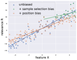
(a) Only one bias

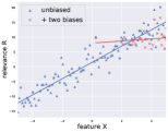
(b) Both two biases

Figure 2. Results of the synthetic study. Points and lines denote the training data and the models, respectively.

3.3. An illustrative synthetic study

To present how these two biases affect our model, we conducted a synthetic experiment and the results are shown in Figure 2(a). Specifically, we simulated a learning to rank dataset which has one dimension feature $x$ for each query-document pair. Based on the synthetic data (blue triangles), an unbiased linear model was estimated (blue line). We added position bias into the dataset, resulting the observed records (orange crosses) which have an offset to the true relevance. Therefore, the learned ranking model (orange line) is biased. Similarly, if we selected the top-$k$ records (green triangles), the learned ranking model (green line) is also biased.

Moreover, two biases can be compounded and make the learned model deviate even severe, as shown in Figure 2(b). As a consequence, just mitigating one bias at a time (e.g., simply ensembling the results (Ovaisi et al., 2020)) still leads to biased results. It is necessary to develop a unified model that can mitigate two biases simultaneously.

4. Unified bias mitigation in top-$k$ ranking

Based on the analysis in the above section, this section presents a model called Causal Likelihood Decomposition (CLD) which simultaneously mitigates the position bias and the sample selection bias in top-$k$ learning to rank.

4.1. Formulation of the log-likelihood

The analysis of Equation (5) in Section 3.1 indicates that the click signals can be transformed to relevance with the help of propensity score: $\mathbb{E}\left[\frac{C}{\mathrm{Pr}(E=1|P=k)}~{}\Big{|}\mathbf{x}\right]=R(\mathbf{x})$. Therefore, the click in Equation (2) can be replaced with the expectation of propensity re-weighted click, achieving a log-likelihood with position bias be detached:

(8) $$\mathcal{L}_{\mathrm{de.}\;\mathrm{posi.}}=\!\!\!\!\sum_{i=1\land s_{i}=1}^{N_{s}}\!\!\!\!\log\left(\mathrm{Pr}\left(\mathbb{E}\left[\frac{c_{i}}{\rho_{i}}\right],s_{i}\bigg{|}\mathbf{x}_{i}\right)\right)+\!\!\!\!\sum_{i=1\land s_{i}=0}^{N_{u}}\!\!\!\!\log\left(\mathrm{Pr}(s_{i}|\mathbf{x}_{i})\right),$$

where $\mathbb{E}\left[\frac{c_{i}}{\rho_{i}}\right]=\mathbb{E}\left[\frac{C}{\mathrm{Pr}(E=1|P=k)}~{}\Big{|}\mathbf{x}\right]$ for simplifying the notations. Note that $\rho_{i}$ is the propensity score for the $i$-th $(q,d)$ pair. A number of studies have been proposed to estimate the weights (Agarwal et al., 2019c; Ai et al., 2018; Wang et al., 2018). In this paper, we treat them as known values.

Equation (8) still suffers sample selection bias because the first term still contains $s_{i}$. As have shown in Equation (7) in Section 3.2, the likelihood of selected data can be decomposed to contain the unbiased learning target, thus detaching sample selection bias:

(9) $$\begin{split}\mathcal{L}_{\mathrm{de.}\;\mathrm{both}\;\mathrm{biases}}&=\sum_{i=1\land s_{i}=1}^{N_{s}}\log\left(\mathrm{Pr}\left(\mathbb{E}\left[\frac{c_{i}}{\rho_{i}}\right]\bigg{|}\mathbf{x}_{i}\right)\right)\\ &+\sum_{i=1\land s_{i}=1}^{N_{s}}\log\left(\mathrm{Pr}\left(s_{i}\bigg{|}~{}\mathbb{E}\left[\frac{c_{i}}{\rho_{i}}\right],\mathbf{x}_{i}\right)\right)\\ &+\sum_{i=1\land s_{i}=0}^{N_{u}}\log\left(\mathrm{Pr}(s_{i}|\mathbf{x}_{i})\right),\end{split}$$

4.2. Optimization

To optimize Equation (9), we followed the Type II Tobit model (Amemiya, 1984), which parameterized the likelihood in Equation (9) under the linear and Gaussian assumptions. Specifically, assuming that both the selection model and the ranking model are linear:

$$s_{i}=\begin{cases}0&\;\mbox{if}\;\mathbf{x}_{i}^{T}\bm{\omega}+\epsilon_{i}\leq 0\\ 1&\;\mbox{if}\;\mathbf{x}_{i}^{T}\bm{\omega}+\epsilon_{i}>0\end{cases},\quad r_{i}=\begin{cases}\mathbf{x}_{i}^{T}\bm{\beta}+\mu_{i}&\;\mbox{if}\;s_{i}=1\\ \mbox{unobserved}&\;\mbox{if}\;s_{i}=0\end{cases},$$

where $s_{i}$ and $r_{i}$ are the selection indicator and the relevance of the $i$-th $(q,d)$, respectively, and both of them are calculated based on the feature vector $\mathbf{x}_{i}$. $\bm{\omega}$ and $\bm{\beta}$ are the parameters of these two linear models. $\epsilon_{i}$ and $\mu_{i}$ are the I.I.D. noises that obey Gaussian distributions and their variances are assumed to be 1.

According to the derivations and conclusions in (Amemiya, 1984), the parameterized log-likelihood of Equation (9) becomes:

(10) $$\begin{split}\mathcal{L}_{\mathrm{CLD}}(\bm{\beta},\bm{\omega})=&-\sum_{i=1\land s_{i}=1}^{N_{s}}\left(\mathbb{E}\left[\frac{c_{i}}{\rho_{i}}\right]-\mathbf{x}_{i}^{T}\bm{\beta}\right)^{2}\\ &+\sum_{i=1\land s_{i}=1}^{N_{s}}\log\Phi\left(\frac{\mathbf{x}_{i}^{T}\bm{\omega}+\gamma\left(\mathbb{E}\left[\frac{c_{i}}{\rho_{i}}\right]-\mathbf{x}_{i}^{T}\bm{\beta}\right)}{(1-\gamma^{2})^{\frac{1}{2}}}\right)\\ &+\sum_{i=1\land s_{i}=0}^{N_{u}}\log\left(1-\Phi(\mathbf{x}_{i}^{T}\bm{\omega})\right),\end{split}$$

where $\Phi$ is the cumulative distribution function of a standard normal distribution, $\gamma$ is the correlation coefficient of the error terms of $\epsilon_{i}$ and $\mu_{i}$, which indicates how the selection of a $(q,d)$ pair related to its relevance. In our implementation, $\gamma$ is treated as a hyper parameter. Maximizing Equation (10) achieves an unbiased estimation of $\bm{\beta}$ and $\bm{\omega}$:

$$(\bm{\beta^{*}},\bm{\omega^{*}})\leftarrow\mathop{\arg\max}_{\bm{\beta},\bm{\omega}}~{}\mathcal{L}_{\mathrm{CLD}}(\bm{\beta},\bm{\omega}).$$

Algorithm 1 shows the procedure of the CLD learning algorithm for learning unbiased relevance ranking model $\bm{\beta}$ (and the selection model $\bm{\omega}$). The inputs to the algorithm are click log with feature, selection indicator, and propensity score re-weighted click signals. After sampling a batch of data, the algorithm updates both models if this data record was selected, and only updates the selection model if it was not selected.

1

Input: iteration number $T$, click log $\mathcal{D}=\mathcal{D}_{s}\bigcup\mathcal{D}_{u}$

2

Output: Model parameters $\bm{\beta}$ and $\bm{\omega}$

3

4$\bm{\rho}\leftarrow$ estimate $K$ propensity scores;

5$\bm{\beta},\bm{\omega}\leftarrow$ Xavier initialization(Glorot and Bengio, 2010);

6 for $1\leq t\leq T$ do

7       Randomly sample a batch of sessions $\mathcal{D^{{}^{\prime}}}$ from $\mathcal{D}_{s}\cup\mathcal{D}_{u}$;

8       for $\left(\mathbf{x}_{i},c_{i},k_{i},s_{i}\right)\in\mathcal{D^{{}^{\prime}}}$ do

9             $\rho_{i}\leftarrow\bm{\rho}[k_{i}]$

10            if $s_{i}=1$ then

11                   Update $\bm{\beta},\bm{\omega}$ with the gradient of Eq. (10) ;

12                  

13            else

14                   Update $\bm{\omega}$ with the gradient of Eq. (10);

15                  

16             end if

17            

18       end for

19      

20 end for

21

return $\bm{\beta},\bm{\omega}$

Algorithm 1 The training procedure of CLD

4.3. Online ranking

The outputs of the learning algorithm are the parameters of the ranking model $\bm{\beta^{*}}$ and parameters of the selection model $\bm{\omega^{*}}$. Intuitively, the selection model is used to absorb the sample selection bias while the relevance model is used to obtain the unbiased estimation of relevance. Therefore, in online ranking, a $(q,d)$ pair’s ranking score is calculated as an unbiased estimation of relevance:

$$\hat{r}=\langle\phi(q,d),\bm{\beta^{*}}\rangle.$$

4.4. Theoretic analysis

Maximizing the propensity re-weighted cumulative rewards has been widely adopted as an effective approach in existing ULTR methods (Joachims and Swaminathan, 2016; Oosterhuis et al., 2020). The proposed CLD, on the other hand, provides a new approach to learning the unbiased ranking model via maximizing the unbiased likelihood of the observed data. The theoretical grantees on the unbiasedness and the variance of CLD are also provided in the following two theorems.

Theorem 1 (Unbiasedness).

$\forall(\mathbf{x}_{i},c_{i},k_{i},s_{i})\in\mathcal{D}$,

$$\begin{split}\mathbb{E}\left[\frac{c_{i}}{\rho_{i}}\right]=r_{i}\Longrightarrow\log\left(\mathrm{Pr}\left(\mathbb{E}\left[\frac{c_{i}}{\rho_{i}}\right]\bigg{|}\mathbf{x}_{i}\right)\right)=\log\left(\mathrm{Pr}(r_{i}|\mathbf{x}_{i})\right).\end{split}$$

The proof of the theorem is straightforward, by directly substituting the term $\mathbb{E}\left[\frac{c_{i}}{\rho_{i}}\right]$ in the right equation with $r_{i}$ in the condition. Theorem 1 indicates that an unbiased ranking model can be obtained via the first term of Equation (9), by maximizing the unified log-likelihood with click log.

Theorem 2 (Variance).

Given a dataset $(\mathbf{x}_{i},c_{i},k_{i},s_{i})\in\mathcal{D}$ and defining $\epsilon=\left(\mathbb{E}\left[\frac{c_{i}}{\rho_{i}}\right]-\mathbf{x}_{i}^{T}\bm{\beta}\right)$, the variance of $\mathcal{L}_{\mathrm{CLD}}$ is:

$$\begin{split}\mathbb{V}\left[\mathcal{L}_{\mathrm{CLD}}\right]=\sum_{i}^{|\mathcal{D}|}\mathbb{V}\left[s_{i}\right]\left(\log\Phi\left(\frac{\mathbf{x}_{i}^{T}\bm{\omega}+\gamma\epsilon}{(1-\gamma^{2})^{\frac{1}{2}}}\right)-\epsilon^{2}+\log\left(1-\Phi(\mathbf{x}_{i}^{T}\bm{\omega})\right)\right)^{2}\end{split}$$

Proof.

The likelihood defined in Equation (10) can be rewritten as the form for a single sample:

$$\begin{split}\mathcal{L}_{\mathrm{CLD}}&=\sum_{i}^{\mathcal{D}}s_{i}\left(\log\Phi\left(\frac{\mathbf{x}_{i}^{T}\bm{\omega}+\gamma\epsilon}{(1-\gamma^{2})^{\frac{1}{2}}}\right)-\epsilon^{2}\right)+(1-s_{i})\log\left(1-\Phi(\mathbf{x}_{i}^{T}\bm{\omega})\right),\end{split}$$

where $\epsilon=\left(\mathbb{E}\left[\frac{c_{i}}{\rho_{i}}\right]-\mathbf{x}_{i}^{T}\bm{\beta}\right)$, for the ease of notation. Since each record in dataset $\mathcal{D}$ is independent, we have:

$$\begin{split}\mathbb{V}\left[\mathcal{L}_{\mathrm{CLD}}\right]&=\mathbb{V}\left[\sum_{i}^{\mathcal{D}}s_{i}\left(\log\Phi\left(\frac{\mathbf{x}_{i}^{T}\bm{\omega}+\gamma\epsilon}{(1-\gamma^{2})^{\frac{1}{2}}}\right)-\epsilon^{2}-\log\left(1-\Phi(\mathbf{x}_{i}^{T}\bm{\omega})\right)\right)\right]\\ &=\sum_{i}^{\mathcal{D}}\mathbb{V}\left[s_{i}\left(\log\Phi\left(\frac{\mathbf{x}_{i}^{T}\bm{\omega}+\gamma\epsilon}{(1-\gamma^{2})^{\frac{1}{2}}}\right)-\epsilon^{2}-\log\left(1-\Phi(\mathbf{x}_{i}^{T}\bm{\omega})\right)\right)\right]\\ &=\sum_{i}^{\mathcal{D}}\mathbb{V}\left[s_{i}\right]\left(\log\Phi\left(\frac{\mathbf{x}_{i}^{T}\bm{\omega}+\gamma\epsilon}{(1-\gamma^{2})^{\frac{1}{2}}}\right)-\epsilon^{2}-\log\left(1-\Phi(\mathbf{x}_{i}^{T}\bm{\omega})\right)\right)^{2}\end{split}$$

∎

It is worth noting that $s_{i}$ is a random variable that obeys the Bernoulli distribution. The other part except $s_{i}$ can be treated as a constant for a given $i$, which is related to input $\mathbf{x_{i}}$. Therefore, the variance of CLD depends on the variance of $s_{i}$ and the scale of input $\mathbf{x_{i}}$. In comparison with IPS, the variance of CLD avoids dividing by propensity, thus avoiding being affected by those extreme minimal propensity values.

Input: iteration number $T$, click log $\mathcal{D}=\mathcal{D}_{s}\bigcup\mathcal{D}_{u}$

Output: Model parameters $\bm{\beta}$, $\bm{\omega}$

1 // Create preference pairs based on $\mathcal{D}$ ;

2

3$\bm{\rho}\leftarrow$ estimate $K$ propensity scores;

4$\mathcal{D}_{s}^{pair}\!\!\!\!\leftarrow\left\{\left((\mathbf{x}_{i},s_{i}),(\mathbf{x}_{j},s_{j})\right)\Big{|}~{}\mathbb{E}\left[\frac{c_{i}}{\bm{\rho}[k_{i}]}\right]>\mathbb{E}\left[\frac{c_{j}}{\bm{\rho}[k_{j}]}\right],s_{i}=1\land s_{j}=1\right\}$;

5

6$\mathcal{D}_{u}^{pair}\!\!\!\!\leftarrow\left\{\left((\mathbf{x}_{i},s_{i}),(\mathbf{x}_{j},s_{j})\right)\Big{|}~{}s_{i}=0\lor s_{j}=0\right\}$;

7

8$\bm{\beta},\bm{\omega}\leftarrow$ Xavier initialization(Glorot and Bengio, 2010);

9 for $1\leq t\leq T$ do

10       Randomly sample a batch $\mathcal{D^{{}^{\prime}}}$ from $\mathcal{D}_{s}^{pair}\cup\mathcal{D}_{u}^{pair}$;

11       for $\left((\mathbf{x}_{i},s_{i}),(\mathbf{x}_{j},s_{j})\right)\in\mathcal{D^{{}^{\prime}}}$ do

12             if $s_{i}=1\lor s_{j}=1$ then

13                   Update $\bm{\beta},\bm{\omega}$ with the gradient of Eq. (13) ;

14                  

15            else

16                   Update $\bm{\omega}$ with the gradient of Eq. (13);

17                  

18             end if

19            

20       end for

21      

22 end for

23return $\bm{\beta},\bm{\omega}$

Algorithm 2 Pairwise training for CLD

5. Extension to pairwise neural ranking

The models learned by Algorithm 1 are limited to be linear and learned with a pointwise objective function. Previous studies have shown that the neural ranking models learned with a pairwise objective such as BPR (Rendle et al., 2012) usually achieve better results. In this section, we extend the proposed pointwise and linear CLD model to pairwise neural ranking, denoted as CLD${}^{\textrm{pair}}$.

To derive the pairwise format of CLD, we first give the unbiased log-likelihood in pairwise format:

(11) $$\begin{split}\mathcal{L}_{\mathrm{unbiased}}^{\mathrm{pair}}&=\sum_{r_{i}>r_{j}}\log\left(\mathrm{Pr}(r_{i}>r_{j}|\mathbf{x}_{i},\mathbf{x}_{j})\right).\end{split}$$

For a document $i$ and document $j$ in the ranking list of query $\bm{q}$, the pairwise unbiased likelihood is consists of the relative order of their relevance comparisons. Unfortunately, the relevance $r_{i}$ and $r_{j}$ is unknown for us. What we can observe is the click signal of each document, Based on Equation (9) and Equation (11), the decomposed log-likelihood in pairwise can be written as

$$\mathcal{L}_{\mathrm{de.}\;\mathrm{both}\;\mathrm{biases}}^{\mathrm{pair}} =\sum_{\bar{r}_{i}>\bar{r}_{j},\;s_{i}=1\land s_{j}=1}\log\left(\mathrm{Pr}(\bar{r}_{i}>\bar{r}_{j}|\mathbf{x}_{i},\mathbf{x}_{j})\right)$$

$$+\sum_{\bar{r}_{i}>\bar{r}_{j},\;s_{i}=1\land s_{j}=1}\log\left(\mathrm{Pr}(s_{i},s_{j}|\bar{r}_{i}>\bar{r}_{j},\mathbf{x}_{i},\mathbf{x}_{j})\right)$$

(12) $$+\sum_{s_{i}=0\lor s_{j}=0}\log\left(\mathrm{Pr}(s_{i},s_{j}|\mathbf{x}_{i},\mathbf{x}_{j})\right),$$

where $\bar{r}_{i}=\mathbb{E}\left[c_{i}/\rho_{i}\right]$ and $\bar{r}_{j}=\mathbb{E}\left[c_{j}/\rho_{j}\right]$. Since $\mathbb{E}\left[c_{i}/\rho_{i}\right]=r_{i}$, the first term of Equation (12) implies an unbiased log-likelihood. Maximizing Equation (12) can obtain an unbiased ranking model.

To conduct the optimization, we first parameterize the models with neural networks, as shown in Figure 3. Given a $(q,d)$ pair, its representation is denoted as $\mathbf{x}$. Based on the representation, the relevance ranking model and selection model are defined as feed-forward neural networks, denoted as $f_{\bm{\beta}}(\cdot)$ and $f_{\bm{\omega}}(\cdot)$, respectively. Furthermore, we assume that in the second and third terms of Equation (12), the selection of document pairs $(\mathbf{x}_{i},\mathbf{x}_{j})$ are independent:

$$\mathrm{Pr}(s_{i},s_{j}|\bar{r}_{i}>\bar{r}_{j},\mathbf{x}_{i},\mathbf{x}_{j}) =\mathrm{Pr}(s_{i}|\bar{r}_{i}>\bar{r}_{j},\mathbf{x}_{i})\mathrm{Pr}(s_{j}|\bar{r}_{i}>\bar{r}_{j},\mathbf{x}_{j});$$

$$\mathrm{Pr}(s_{i},s_{j}|\mathbf{x}_{i},\mathbf{x}_{j}) =\mathrm{Pr}(s_{i}|\mathbf{x}_{i})\mathrm{Pr}(s_{j}|\mathbf{x}_{j}).$$

Figure 3. The unified debiasing model structure for optimizing pairwise neural format of CLD.

As shown in Figure 3(a), if both of the documents in a pair are selected into the top-$k$ positions, the likelihood of relevance part and conditional selection part can be formulated with BPR loss and Binary Cross Entropy loss, respectively. if only one document in a pair is selected, the conditional selection likelihood can be approximated as that shown in Figure 3(b). If neither of the two documents in a pair is selected, the selection likelihood can be formulated with Binary Cross Entropy loss directly (Figure 3(c)). Therefore, the overall pairwise objective function becomes:

(13) $$\hphantom{{}={}}\mathcal{O}_{\mathrm{CLD}}^{\mathrm{pair}}(\bm{\beta},\bm{\omega})=s_{i}s_{j}\log~{}\sigma\left(f_{\bm{\beta}}(\mathbf{x}_{i})-f_{\bm{\beta}}(\mathbf{x}_{j})\right)$$

$$+s_{i}\log~{}\sigma\left(f_{\bm{\omega}}(\mathbf{x}_{i})+f_{\bm{\beta}}(\mathbf{x}_{i})-f_{\bm{\beta}}(\mathbf{x}_{j})\right)+(1-s_{i})\log~{}\sigma\left(1-f_{\bm{\omega}}(\mathbf{x}_{i})\right)$$

$$+s_{j}\log~{}\sigma\left(f_{\bm{\omega}}(\mathbf{x}_{j})+f_{\bm{\beta}}(\mathbf{x}_{i})-f_{\bm{\beta}}(\mathbf{x}_{j})\right)+(1-s_{j})\log~{}\sigma\left(1-f_{\bm{\omega}}(\mathbf{x}_{j})\right),$$

where $\sigma$ denotes the sigmoid function. To maximize Equation (13), we can get the approximately unbiased estimation of $\bm{\beta}$ and $\bm{\omega}$:

$$(\bm{\beta^{*}},\bm{\omega^{*}})\leftarrow\mathop{\arg\max}_{\bm{\beta},\bm{\omega}}~{}\mathcal{O}_{\mathrm{CLD}}^{\mathrm{pair}}(\bm{\beta},\bm{\omega}).$$

Algorithm 2 illustrates the optimization procedure for Equation (13).

As for online ranking, given a $(q,d)$ pair, its ranking score is calculated by the ranking model $f_{\bm{\beta^{*}}}$:

$$\hat{r}=f_{\bm{\beta^{*}}}(\phi(q,d)).$$

6. Experiment setup

We conducted experiments to evaluate the proposed CLD and its extension CLD${}^{\textrm{pair}}$, by following the settings presented in the existing unbiased learning to rank studies (Joachims et al., 2017; Ai et al., 2018; Agarwal et al., 2019a; Oosterhuis and de Rijke, 2020).

Datasets: Two widely used public datasets, YaHooC14B (Chapelle and Chang, 2011) and WEB10K (Qin and Liu, 2013), were used in our experiments. YaHooC14B contains around 30,000 queries, each associated with averaged of 24 documents. Each query-document pair is depicted with a 700-dimension feature vector and five-grade relevance labels. WEB10K has 10,000 queries and each associated with about 125 documents. Each query-document pair is depicted with a 136-dimension feature vector and a five-grade relevance label. Following the practices in (Joachims et al., 2017), we converted the relevance label in both two datasets with $r=1$ for grades 3 and 4 and $r=0$ for the others. Only the set 1 of YaHooC14B and the first fold of WEB10K was used for training. Expert annotated labels in the test sets were used to evaluate the ranking accuracy.

Click simulation: Following the practices in (Joachims et al., 2017), the users’ interactions with search engines were simulated and got the clicks. First, 1% labeled data were randomly sampled from the dataset and used to train an SVM^rank(Joachims, 2002) as the production ranker. Then for each click session, a query was uniformly sampled and the ranking result was generated by the production ranker. To simulate users’ click, the position based model (PBM) (Richardson et al., 2007; Ai et al., 2021) was adopted in which $(E=1\wedge R=1)\Rightarrow C=1$, a click occurs only when the document is examined and is relevant. For every $(q,d)$ pair, the examination probability is based on the displayed position:

(14) $$\mathrm{Pr}(E=1|P=k)=\begin{cases}\left(\frac{1}{k}\right)^{\eta},&\mbox{if\;}k\leq K\\ 0,&\mathrm{else}\end{cases}$$

where $\eta$ is the parameter to control the severity of position bias, and $K$ is the cut-off position. The examination probability is also the propensity score in the proposed approach and we assume it is known in advance. During the process, the irrelevant documents were allowed to be clicked with a small probability to simulate the click noise.

Baselines: State-of-the-art unbiased learning to rank approaches were adopted as the baselines:

Naive:

: Directly regarding the clicks as relevance labels.

IPS (Joachims et al., 2017):

: Correcting the position bias with propensity score.

Heckman${}^{\textrm{rank}}$ (Ovaisi et al., 2020):

: Correcting the sample selection bias with Heckman two-stage method.

RankAgg(Ovaisi et al., 2020):

: Mitigating both the position bias and sample selection bias by combining the results of IPS and Heckman${}^{\textrm{rank}}$.

Oracle:

: Using the non-discarded expert annotated labels to learn the ranking model. It showed the (theoretical) performance upper bound on the dataset.

Policy-aware IPS (Oosterhuis and de Rijke, 2020) was not chosen as a baseline because it assumes the previous ranking models should be stochastic, which violets the Assumption (1).

Evaluation metric: NDCG@1, NDCG@3, and MAP were used to evaluate the accuracy of the baselines and the proposed method.

Implementation details: Similar to existing studies (Ai et al., 2018; Agarwal et al., 2019a; Vardasbi et al., 2020), we used a three layers neural networks with $elu$ activation function as the ranking model for Naive, IPS, Oracle and CLD${}^{\textrm{pair}}$, with the hidden sizes $[256,128,64]$, and dropout probability of $0.5$. For Heckman${}^{\textrm{rank}}$ and CLD (pointwise and linear), the ranking model was set to linear. The selection models for CLD and CLD${}^{\textrm{pair}}$ were also set to linear. The learning rate were tuned among $\{2e{-4},5e{-4},1e{-3},2e{-3},5e{-3}\}$. The $L2$ regularization was used and the trade-off factor was tuned between $[1e{-3},1e{-2}]$. The correlation $\gamma$ in Equation (10) was tuned between $[0.05,0.30]$. In all of the experiments, the reported numbers were the averaged results after training 12 epochs with 5 different random seeds.

The source code, data, and experiments will be available at https://github.com/hide_for_blind_review

7. Results and discussions

Table 2. Ranking accuracy on YaHooC14B and WEB10K. Boldface means the best performed approaches (excluding Oracle). Experimental settings: top-5 cut-off, $\mathbf{\eta=0.1}$, $10^{5}$ click sessions, and 10% click noise. We also present the 90% confidence interval of $t$-distribution for our methods.

Method	YaHooC14B			WEB10K
	NDCG@1	NDCG@3	MAP	NDCG@1	NDCG@3	MAP
Naive	0.606	0.593	0.592	0.383	0.350	0.294
IPS	0.650	0.619	0.609	0.413	0.368	0.282
$\mathrm{Heckman}^{\mathrm{rank}}$	0.608	0.590	0.587	0.350	0.331	0.287
RankAgg	0.649	0.623	0.608	0.413	0.375	0.299
$\mathrm{CLD}$	$0.661\pm.002$	$\mathbf{0.631\pm.001}$	$\mathbf{0.616\pm.001}$	$0.434\pm.005$	$0.391\pm.003$	$0.312\pm.001$
$\mathrm{CLD}^{\mathrm{pair}}$	$\mathbf{0.662\pm.001}$	$0.630\pm.001$	$0.615\pm.001$	$\mathbf{0.439\pm.001}$	$\mathbf{0.397\pm.001}$	$\mathbf{0.312\pm.000}$
Oracle	0.666	0.636	0.622	0.455	0.416	0.332

Table 2 shows the ranking accuracy of our approaches and the baselines, on YaHooC14B and WEB10K. The results showed that the proposed CLD and CLD${}^{\textrm{pair}}$ outperformed the baselines in terms of NDCG and MAP. “Oracle” is the upper bound of the performance, since it uses expert annotated labels. The results verified the effectiveness of the unified bias mitigation in top-k ranking.

Figure 4. Performance curves of different methods w.r.t. bias severity levels. Experimental settings: $10^{5}$ click sessions, and 10% click noise. Shaded area indicates the 90% confidence intervals of $t$-distribution. Left two figures: performance curves w.r.t. different severity of sampling selection bias. Right two figures: performance curves w.r.t. different severity of position bias.

To further reveal how CLD and CLD${}^{\text{pair}}$ outperformed the baselines, we conducted a group of exploratory experiments to answer the following research questions:

• How does CLD perform under different severity levels of sample selection bias and position bias?

• How does CLD perform under different scales of click data?

• Is CLD robust to click noise?

• Is CLD robust to misspecified propensity score?

• How does CLD perform with different base model?

7.1. The effect of biases severity (RQ1)

To varying the severity levels of sample selection bias, we changed the ranking cut-off position $k$ from 2 to 20. Smaller $k$ leads to more severe sample selection bias. The left two sub-figures of Figure (4) show the performance curves of different approaches w.r.t. different $k$ values. From the results, we can see that in general CLD and CLD${}^{\textrm{pair}}$ outperformed the baselines at all of the $k$ values (except CLD when $k>10$ on WEB10K). On both datasets, when $k$ was small , CLD and CLD${}^{\textrm{pair}}$ outperformed the baselines with a large margin and achieved the performance closing to the upper bound. With the increasing of $k$, the improvements of CLD and CLD${}^{\textrm{pair}}$ over IPS gradually become limited. This is because sample selection bias gets milder for larger $k$, making position bias dominates the negative effects of bias. Similar performance curves also came to RankAgg, another model which can mitigate both position bias and sample selection bias.

On the contrary, increasing $k$ will lead to the performance drop of naive methods. This is because the naive method can handle neither of these two biases. Increasing data will not further improve its performance but decrease its performance instead. Also note that CLD${}^{\textrm{pair}}$ outperformed CLD on WEB10K since it learns a neural ranking model based on the pairwise loss. However, all methods can achieve relatively high performances on YaHooC14B. The spaces for further improvement are limited, leading to similar performances for CLD${}^{\textrm{pair}}$ and CLD.

To change the severity levels of position bias, we tuned the the parameter $\eta$ in Equation (14) from 0.0 to 2.0. Larger $\eta$ leads to more severe position bias. The right two sub-figures in Figure 4 illustrate the performances curves w.r.t. different $\eta$ values. From the results, we can see that CLD and CLD${}^{\textrm{pair}}$ still outperformed all the baselines on both datasets. With the increasing of $\eta$, the methods that can correct position bias (except Heckman${}^{\textrm{rank}}$ and Naive) have slight performance drops. Among the baselines, Heckman${}^{\textrm{rank}}$ achieved the higher performance when $\eta=0$ (no position bias), but dropped rapidly when $\eta$ increases. RankAgg also suffered from the performance drop with the increasing $\eta$ because it is an ensemble of Heckman${}^{\textrm{rank}}$. The phenomenon confirmed the conclusion in Section 3.3: only mitigating one bias separately still leads to a biased result in top-$k$ ranking. Simply aggregating the results outputted by the methods that only correct one bias still leads to biased results.

Figure 5. Performance curves of different methods w.r.t. the number of click sessions. Experimental settings: top-5 cut-off, $\mathbf{\eta=1.0}$ and 10% click noise.

Figure 6. Performance curves of different methods w.r.t. click noise severity levels. Experimental settings: top-5 cut-off, $\mathbf{\eta=1.0}$ and trained with $10^{5}$ click sessions.

7.2. The effects of click scales (RQ2)

We tested the performances of different methods by varying the scale of the click data. Figure 5 illustrates the performance curves of different methods w.r.t. the number of click sessions used for training the models. The results indicate that both CLD and CLD${}^{\textrm{pair}}$ consistently outperformed the baseline methods over different click session scales. According to Equation (10) and (13), CLD and CLD${}^{\textrm{pair}}$ have the ability of utilizing the unobserved data in training. The ability makes them perform well even being trained with a limited number of click sessions. With more click sessions being involved in training, the performances of CLD and CLD${}^{\textrm{pair}}$ steadily improved. In contrast, IPS and Heckman${}^{\textrm{rank}}$ can only correct one bias in top-$k$ ranking. Therefore, with the increasing number of click sessions used for training, they underperformed those methods that can mitigate both position bias and sample selection bias (e.g., RankAgg, CLD and CLD${}^{\textrm{pair}}$). All these results clearly verified the advantages of the proposed unified bias mitigation.

7.3. The effects of click noises (RQ3)

We also conducted experiments with variant noise levels in the clicks, by changing the probability of clicking irrelevant documents from 0.0 to 0.5 when generating the training data. According to the results shown in Figure 6, both CLD and CLD${}^{\textrm{pair}}$ outperformed the baselines at different noise levels, indicating the robustness of the unified bias mitigation approach. Particularly, among all of the methods, CLD has minimal performance drops.

We analyzed the reasons and found that each noise click will produce more mistake pairs in pairwise methods than that of in pointwise methods. Therefore, when training with these mistake pairs, pairwise method will be suffered more. However, for pointwise method, each noise click is only presented once in the training set, making it more robust than the pairwise models.

Figure 7. Performance curves of different methods on YaHooC14B w.r.t. degrees of misspecified propensity scores in different top-k cut-offs. The true $\mathbf{\eta}=1$ and click noise is 10%.

7.4. Effects of misspecified propensity score (RQ4)

The result we reported before assumes that the model knows the true propensity score, which is often difficult in the real world. In this experiment, we conducted experiments to test the performance of each method under various degrees on misspecified propensity scores and different top-$k$ cut-offs, characterized by parameters $\eta$ and $k$, respectively. The true value $\eta=1$ and we varied it in $[0.0,2.0]$. We tested the cases when $k=3$ and $k=5$. Note that Heckman${}^{\textrm{rank}}$ are not considered as a baseline in this experiment. This is because Heckman${}^{\textrm{rank}}$ does not use propensity scores.

Figure 7 illustrates the performance curves of CLD, CLD^pair, IPS, and RankAgg on YaHooC14B, under various degrees of misspecified propensity scores. The left and right figures respectively illustrate the results when $k=3$ and $k=5$. From the results, we can see that in general CLD outperformed the best in all degrees of misspecified propensity scores, which indicates the robustness of CLD. When the propensity was overestimated (i.e., $\eta<1$), all methods related to propensity score only have a slight performance drop. However, all methods have violent performance drops if the propensity was underestimated (i.e., $\eta>1$). This is because when the propensity is underestimated, the estimated propensity becomes smaller than its true value, and thus increasing the variance of propensity re-weighting. Even when the propensity was underestimated, the proposed CLD still outperformed other methods with large margins. As have stated in Theorem 2, the variance of CLD avoids dividing by propensity score and therefore can reduce the variance caused by the underestimation of the propensity. Moreover, we found that the effects of misspecified propensity scores were more severe on large $k$. This is because the larger the ranking positions, the more suffers come from the position bias.

Table 3. Ranking accuracy comparison among different variants of CLD on YaHooC14B and WEB10K. Boldface means the best performed approaches (excluding Oracle). Experimental settings: top-5 cut-off, $\mathbf{\eta=0.1}$, $10^{5}$ click sessions, and 10% click noise.

Method	YaHooC14B			WEB10K
	NDCG@1	NDCG@3	MAP	NDCG@1	NDCG@3	MAP
CLD	0.661	0.631	0.616	0.434	0.391	0.312
CLD-N	0.652	0.619	0.610	0.340	0.321	0.284
CLD${}^{\textrm{pair}}$	0.662	0.630	0.615	0.439	0.397	0.312
CLD${}^{\textrm{pair}}$-L	0.660	0.634	0.618	0.431	0.389	0.309
Oracle	0.666	0.636	0.622	0.455	0.416	0.332

7.5. The effects of base model (RQ5)

In previous experiments, CLD was designed as a linear ranking model because of its theoretic grantees, while CLD${}^{\textrm{pair}}$ was designed to use nonlinear neural networks as its ranker. In this experiment, we modified these models so that CLD was based on a neural network with three hidden layers and CLD${}^{\textrm{pair}}$ used a linear model as the ranker, denoted as CLD-N and CLD${}^{\textrm{pair}}$-L, respectively.

Table 3 reports the ranking accuracy of CLD, CLD${}^{\textrm{pair}}$, and their variations, on YaHooC14B and WEB10K. From the results, we found that (1) CLD-N performed worst among these methods, especially on WEB10K. Compared to CLD, CLD-N used a nonlinear neural network as its ranker, which makes it lose the theoretical guarantees; (2) CLD${}^{\textrm{pair}}$ outperformed CLD${}^{\textrm{pair}}$-L on WEB10K and performed comparably on YaHooC14B. Please note that WEB10K is larger than YaHooC14B and all methods can achieve relatively scores on YaHooC14B. We concluded that using a linear model in CLD and using nonlinear neural networks in CLD${}^{\textrm{pair}}$ are reasonable settings.

8. Conclusions

In this paper, we have proposed a novel and theoretical sound model for learning unbiased ranking models in top-$k$ learning to rank, referred to as CLD. In contrast to existing methods, CLD simultaneously tackles the position bias and sampling selection biases from the viewpoint of a causal graph. It decomposes the log-likelihood function of user interactions as an unbiased relevance term plus other terms that model the biases. An unbiased ranking model can be obtained by maximizing the whole log-likelihood. Extension to the pairwise neural ranking is also developed. Experimental results verified the superiority of the proposed methods over the baselines in terms of ranking accuracy and robustness.

References

- (1)
- Agarwal et al. (2019a) Aman Agarwal, Kenta Takatsu, Ivan Zaitsev, and Thorsten Joachims. 2019a. A General Framework for Counterfactual Learning-to-Rank. In Proceedings of the 42nd International ACM SIGIR Conference on Research and Development in Information Retrieval. ACM, 5–14.
- Agarwal et al. (2019b) Aman Agarwal, Xuanhui Wang, Cheng Li, Michael Bendersky, and Marc Najork. 2019b. Addressing Trust Bias for Unbiased Learning-to-Rank. In The World Wide Web Conference. ACM, 4–14.
- Agarwal et al. (2019c) Aman Agarwal, Ivan Zaitsev, Xuanhui Wang, Cheng Li, Marc Najork, and Thorsten Joachims. 2019c. Estimating Position Bias without Intrusive Interventions. In Proceedings of the Twelfth ACM International Conference on Web Search and Data Mining. ACM, 474–482.
- Ai et al. (2018) Qingyao Ai, Keping Bi, Cheng Luo, Jiafeng Guo, and W. Bruce Croft. 2018. Unbiased Learning to Rank with Unbiased Propensity Estimation. In The 41st International ACM SIGIR Conference on Research Development in Information Retrieval. ACM, 385–394.
- Ai et al. (2021) Qingyao Ai, Tao Yang, Huazheng Wang, and Jiaxin Mao. 2021. Unbiased Learning to Rank: Online or Offline? ACM Trans. Inf. Syst. 39, 2, Article 21 (Feb. 2021), 29 pages.
- Amemiya (1984) T. Amemiya. 1984. Tobit models: A survey. Journal of Econometrics 24, 1-2 (1984).
- Carterette and Chandar (2018) Ben Carterette and Praveen Chandar. 2018. Offline Comparative Evaluation with Incremental, Minimally-Invasive Online Feedback. In The 41st International ACM SIGIR Conference on Research Development in Information Retrieval. ACM, 705–714.
- Chapelle and Chang (2011) Olivier Chapelle and Yi Chang. 2011. Yahoo! learning to rank challenge overview. In Proceedings of the learning to rank challenge. PMLR, 1–24.
- Chen et al. (2021) Jiawei Chen, Hande Dong, Yang Qiu, Xiangnan He, Xin Xin, Liang Chen, Guli Lin, and Keping Yang. 2021. AutoDebias: Learning to Debias for Recommendation. In Proceedings of the 44th International ACM SIGIR Conference on Research and Development in Information Retrieval. ACM, 21–30.
- Chen et al. (2020) Jiawei Chen, Hande Dong, Xiang Wang, Fuli Feng, Meng Wang, and Xiangnan He. 2020. Bias and debias in recommender system: A survey and future directions. arXiv preprint arXiv:2010.03240 (2020).
- Cole et al. (2010) Stephen R Cole, Robert W Platt, Enrique F Schisterman, Haitao Chu, Daniel Westreich, David Richardson, and Charles Poole. 2010. Illustrating bias due to conditioning on a collider. International journal of epidemiology 39, 2 (2010), 417–420.
- Craswell et al. (2008) Nick Craswell, Onno Zoeter, Michael Taylor, and Bill Ramsey. 2008. An Experimental Comparison of Click Position-Bias Models. In Proceedings of the 2008 International Conference on Web Search and Data Mining. ACM, 87–94.
- Dong et al. (2020) Zhenhua Dong, Hong Zhu, Pengxiang Cheng, Xinhua Feng, Guohao Cai, Xiuqiang He, Jun Xu, and Jirong Wen. 2020. Counterfactual learning for recommender system. In Fourteenth ACM Conference on Recommender Systems. 568–569.
- Fang et al. (2019) Zhichong Fang, Aman Agarwal, and Thorsten Joachims. 2019. Intervention Harvesting for Context-Dependent Examination-Bias Estimation. In Proceedings of the 42nd International ACM SIGIR Conference on Research and Development in Information Retrieval. ACM, 825–834.
- Glorot and Bengio (2010) Xavier Glorot and Yoshua Bengio. 2010. Understanding the difficulty of training deep feedforward neural networks. In Proceedings of the thirteenth international conference on artificial intelligence and statistics. JMLR Workshop and Conference Proceedings, 249–256.
- Heckman (1976) James J Heckman. 1976. The common structure of statistical models of truncation, sample selection and limited dependent variables and a simple estimator for such models. In Annals of economic and social measurement. NBER, 475–492.
- Heckman (1979) James J Heckman. 1979. Sample selection bias as a specification error. Econometrica: Journal of the econometric society (1979), 153–161.
- Hu et al. (2019) Ziniu Hu, Yang Wang, Qu Peng, and Hang Li. 2019. Unbiased LambdaMART: An Unbiased Pairwise Learning-to-Rank Algorithm. In The World Wide Web Conference. ACM, 2830–2836.
- Jagerman et al. (2019) Rolf Jagerman, Harrie Oosterhuis, and Maarten de Rijke. 2019. To Model or to Intervene: A Comparison of Counterfactual and Online Learning to Rank from User Interactions. In Proceedings of the 42nd International ACM SIGIR Conference on Research and Development in Information Retrieval. ACM, 15–24.
- Jeunen et al. (2020) Olivier Jeunen, David Rohde, Flavian Vasile, and Martin Bompaire. 2020. Joint Policy-Value Learning for Recommendation. In Proceedings of the 26th ACM SIGKDD International Conference on Knowledge Discovery Data Mining. ACM, 1223–1233.
- Joachims (2002) Thorsten Joachims. 2002. Optimizing Search Engines Using Clickthrough Data. In Proceedings of the Eighth ACM SIGKDD International Conference on Knowledge Discovery and Data Mining. Association for Computing Machinery, 133–142.
- Joachims et al. (2005) Thorsten Joachims, Laura Granka, Bing Pan, Helene Hembrooke, and Geri Gay. 2005. Accurately Interpreting Clickthrough Data as Implicit Feedback. In Proceedings of the 28th Annual International ACM SIGIR Conference on Research and Development in Information Retrieval. ACM, 154–161.
- Joachims et al. (2007) Thorsten Joachims, Laura Granka, Bing Pan, Helene Hembrooke, Filip Radlinski, and Geri Gay. 2007. Evaluating the Accuracy of Implicit Feedback from Clicks and Query Reformulations in Web Search. ACM Trans. Inf. Syst. 25, 2 (2007), 7–es.
- Joachims and Swaminathan (2016) Thorsten Joachims and Adith Swaminathan. 2016. Counterfactual Evaluation and Learning for Search, Recommendation and Ad Placement. In Proceedings of the 39th International ACM SIGIR Conference on Research and Development in Information Retrieval. ACM, 1199–1201.
- Joachims et al. (2017) Thorsten Joachims, Adith Swaminathan, and Tobias Schnabel. 2017. Unbiased Learning-to-Rank with Biased Feedback. In Proceedings of the Tenth ACM International Conference on Web Search and Data Mining. ACM, 781–789.
- Niu et al. (2012) Shuzi Niu, Jiafeng Guo, Yanyan Lan, and Xueqi Cheng. 2012. Top-k Learning to Rank: Labeling, Ranking and Evaluation. In Proceedings of the 35th International ACM SIGIR Conference on Research and Development in Information Retrieval. ACM, 751–760.
- Oosterhuis and de Rijke (2020) Harrie Oosterhuis and Maarten de Rijke. 2020. Policy-Aware Unbiased Learning to Rank for Top-k Rankings. In Proceedings of the 43rd International ACM SIGIR Conference on Research and Development in Information Retrieval. ACM, 489–498.
- Oosterhuis and de Rijke (2021a) Harrie Oosterhuis and Maarten de Rijke. 2021a. Unifying Online and Counterfactual Learning to Rank: A Novel Counterfactual Estimator That Effectively Utilizes Online Interventions. In Proceedings of the 14th ACM International Conference on Web Search and Data Mining. ACM, 463–471.
- Oosterhuis and de Rijke (2021b) Harrie Oosterhuis and Maarten de de Rijke. 2021b. Robust Generalization and Safe Query-Specializationin Counterfactual Learning to Rank. In Proceedings of the Web Conference 2021. Association for Computing Machinery, 158–170.
- Oosterhuis et al. (2020) Harrie Oosterhuis, Rolf Jagerman, and Maarten de Rijke. 2020. Unbiased Learning to Rank: Counterfactual and Online Approaches. In Companion Proceedings of the Web Conference 2020. ACM, 299–300.
- Ovaisi et al. (2020) Zohreh Ovaisi, Ragib Ahsan, Yifan Zhang, Kathryn Vasilaky, and Elena Zheleva. 2020. Correcting for Selection Bias in Learning-to-Rank Systems. In Proceedings of The Web Conference 2020. ACM, 1863–1873.
- Ovaisi et al. (2021) Zohreh Ovaisi, Kathryn Vasilaky, and Elena Zheleva. 2021. Propensity-Independent Bias Recovery in Offline Learning-to-Rank Systems. In Proceedings of the 44th International ACM SIGIR Conference on Research and Development in Information Retrieval. ACM, 1763–1767.
- Pearl (2009) Judea Pearl. 2009. Causality. Cambridge university press.
- Qin and Liu (2013) Tao Qin and Tie-Yan Liu. 2013. Introducing LETOR 4.0 datasets. arXiv preprint arXiv:1306.2597 (2013).
- Rendle et al. (2012) Steffen Rendle, Christoph Freudenthaler, Zeno Gantner, and Lars Schmidt-Thieme. 2012. BPR: Bayesian personalized ranking from implicit feedback. arXiv preprint arXiv:1205.2618 (2012).
- Richardson et al. (2007) Matthew Richardson, Ewa Dominowska, and Robert Ragno. 2007. Predicting Clicks: Estimating the Click-through Rate for New Ads. ACM, 521–530.
- Saito (2020) Yuta Saito. 2020. Asymmetric Tri-Training for Debiasing Missing-Not-At-Random Explicit Feedback. In Proceedings of the 43rd International ACM SIGIR Conference on Research and Development in Information Retrieval. ACM, 309–318.
- Schnabel et al. (2016) Tobias Schnabel, Adith Swaminathan, Ashudeep Singh, Navin Chandak, and Thorsten Joachims. 2016. Recommendations as treatments: Debiasing learning and evaluation. In international conference on machine learning. PMLR, 1670–1679.
- Storkey (2009) Amos Storkey. 2009. When training and test sets are different: characterizing learning transfer. Dataset shift in machine learning 30 (2009), 3–28.
- Vardasbi et al. (2020) Ali Vardasbi, Harrie Oosterhuis, and Maarten de Rijke. 2020. When Inverse Propensity Scoring Does Not Work: Affine Corrections for Unbiased Learning to Rank. In Proceedings of the 29th ACM International Conference on Information Knowledge Management. ACM, 1475–1484.
- Wang et al. (2021) Wenjie Wang, Fuli Feng, Xiangnan He, Xiang Wang, and Tat-Seng Chua. 2021. Deconfounded Recommendation for Alleviating Bias Amplification. In Proceedings of the 27th ACM SIGKDD Conference on Knowledge Discovery Data Mining. Association for Computing Machinery, 1717–1725.
- Wang et al. (2016) Xuanhui Wang, Michael Bendersky, Donald Metzler, and Marc Najork. 2016. Learning to Rank with Selection Bias in Personal Search. In Proceedings of the 39th International ACM SIGIR Conference on Research and Development in Information Retrieval. ACM, 115–124.
- Wang et al. (2018) Xuanhui Wang, Nadav Golbandi, Michael Bendersky, Donald Metzler, and Marc Najork. 2018. Position Bias Estimation for Unbiased Learning to Rank in Personal Search. In Proceedings of the Eleventh ACM International Conference on Web Search and Data Mining. ACM, 610–618.
- Wang et al. (2019) Xiaojie Wang, Rui Zhang, Yu Sun, and Jianzhong Qi. 2019. Doubly robust joint learning for recommendation on data missing not at random. In International Conference on Machine Learning. PMLR, 6638–6647.
- Wang et al. (2020) Yixin Wang, Dawen Liang, Laurent Charlin, and David M. Blei. 2020. Causal Inference for Recommender Systems. In Fourteenth ACM Conference on Recommender Systems. ACM, 426–431.
- Wei et al. (2021) Tianxin Wei, Fuli Feng, Jiawei Chen, Ziwei Wu, Jinfeng Yi, and Xiangnan He. 2021. Model-Agnostic Counterfactual Reasoning for Eliminating Popularity Bias in Recommender System. In Proceedings of the 27th ACM SIGKDD Conference on Knowledge Discovery Data Mining. Association for Computing Machinery, 1791–1800.
- Yuan et al. (2020) Bowen Yuan, Yaxu Liu, Jui-Yang Hsia, Zhenhua Dong, and Chih-Jen Lin. 2020. Unbiased Ad Click Prediction for Position-Aware Advertising Systems. In Fourteenth ACM Conference on Recommender Systems. ACM, 368–377.
- Zhang et al. (2021) Yang Zhang, Fuli Feng, Xiangnan He, Tianxin Wei, Chonggang Song, Guohui Ling, and Yongdong Zhang. 2021. Causal Intervention for Leveraging Popularity Bias in Recommendation. In Proceedings of the 44th International ACM SIGIR Conference on Research and Development in Information Retrieval. ACM, 11–20.
- Zheng et al. (2021) Yu Zheng, Chen Gao, Xiang Li, Xiangnan He, Yong Li, and Depeng Jin. 2021. Disentangling User Interest and Conformity for Recommendation with Causal Embedding. In Proceedings of the Web Conference 2021. ACM, 2980–2991.
- Zhuang et al. (2021) Honglei Zhuang, Zhen Qin, Xuanhui Wang, Michael Bendersky, Xinyu Qian, Po Hu, and Dan Chary Chen. 2021. Cross-Positional Attention for Debiasing Clicks. In Proceedings of the Web Conference 2021. Association for Computing Machinery, 788–797.