Amplitude and phase fluctuations of gravitational waves magnified by strong gravitational lensing

Abstract

We discuss how small-scale density perturbations on the Fresnel scale affect amplitudes and phases of gravitational waves that are magnified by gravitational lensing in geometric optics. We derive equations that connect the small-scale density perturbations with the amplitude and phase fluctuations to show that such perturbative wave optics effects are significantly boosted in the presence of macro model magnifications such that amplitude and phase fluctuations can easily be observed for highly magnified gravitational waves. We discuss expected signals due to microlensing by stars, dark matter substructure, fuzzy dark matter, and primordial black holes.

I Introduction

The first direct observation of gravitational waves from a compact binary merger in 2015 opened a new window to study the Universe [1]. One of the unique characteristics of gravitational waves from compact binary mergers is that their wavelengths are typically much longer than those of any electromagnetic observations. The longer wavelengths indicate that wave optics effects in the propagation of gravitational waves can become more important, unlike electromagnetic observations for which the geometric optics approximation can safely be used in most cases. Indeed, it has been shown that wave optics effects play a key role in predicting gravitational lensing effects on gravitational waves in several cases (see e.g., [2, 3] for reviews).

When wave optics effects are relevant, the propagation of gravitational waves is barely affected by any structures smaller than the Fresnel scale due to the diffraction. Since the Fresnel scale [4, 5] depends on the frequency of gravitational waves as $\propto f^{-1/2}$, the amplification factor due to gravitational lensing depends also on the frequency in wave optics. Therefore, by checking the frequency evolution of gravitational waveforms we can in principle identify the signature of wave optics gravitational lensing for an ensemble of events or even for a single event (e.g., [6]).

With this situation in mind, Takahashi [5] proposed a novel method to probe small-scale density fluctuations from amplitude and phase fluctuations of gravitational waves. Adopting the Born approximation [7], simple relations between the matter power spectrum and amplitude and phase fluctuations are derived. Oguri and Takahashi [8] extended this work and explored the possibility of using amplitude and phase fluctuations as a probe of dark low-mass halos and primordial black holes. Inamori and Suyama [9] reported a simple universal relation between amplitude and phase fluctuations.

In this paper, we ask how wave optics effects modify amplitudes and phases of gravitational waves magnified by strong gravitational lensing due to normal galaxies or clusters of galaxies. Observing such strong lensing events is expected to be within a reach of ongoing ground experiments (e.g., [10, 11, 12, 13, 14, 15, 16, 17, 18, 19, 20, 21]), for which the geometric optics approximation can be safely used. Wave optics effects on multiple images due to microlensing by stars have been studies in detail [22, 23, 24, 25]. Here we derive simple analytic expressions that connect amplitude and phase fluctuations and small-scale density fluctuations on the Fresnel scale in such situations. We show how the macro model magnification enhances the amplitude and phase fluctuations such that they can be easily detected when the images are highly magnified.

This paper is organized as follows. In Sec. II we derive expressions of amplitude and phase fluctuations in the presence of the macro model magnification. In Sec. III we discuss amplitude and phase fluctuations computed by our formalism, including calculations of expected signals in several models. We summarize our results in Sec. IV. Throughout the paper we assume a flat Universe with the matter density $\Omega_{M}=0.3$, the cosmological constant $\Omega_{\Lambda}=0.7$, and the dimensionless Hubble constant $h=0.7$.

II Derivation

II.1 Complex amplification factor in the presence of small-scale perturbations

We define a complex amplification factor $F$ by the ratio of waveforms with and without gravitational lensing for monochromatic waves $\psi(\bm{x},t)=\tilde{\psi}(\bm{x})e^{-2\pi ift}$ with frequency $f$. Specifically,

$$F=\frac{\tilde{\psi}^{\rm L}}{\tilde{\psi}},$$ (1)

where $\tilde{\psi}$ denotes the original waveform without gravitational lensing and $\tilde{\psi}^{\rm L}$ is the observed amplitude including gravitational lensing effects. For simplicity, throughout the paper we consider gravitational lensing effects in a single thin lens plane at redshift $z$. Under the flat sky approximation, the complex amplification factor is described by (e.g., [2, 3])

$$F_{0}(f,\bm{q}_{\beta})=\frac{\chi_{\rm s}}{c\chi(\chi_{\rm s}-\chi)}\frac{f}{i}\int d\bm{q}\,e^{2\pi if\Delta t_{0}(\bm{q},\bm{q}_{\beta})},$$ (2)

$$\Delta t_{0}(\bm{q},\bm{q}_{\beta})=\frac{\chi_{\rm s}}{c\chi(\chi_{\rm s}-\chi)}\left[\frac{(\bm{q}-\bm{q}_{\beta})^{2}}{2}-\phi_{0}(\bm{q})\right],$$ (3)

where $\chi$ and $\chi_{\rm s}$ are comoving radial distances to the lens and the source, respectively, $\bm{q}$ denotes the comoving two-dimensional coordinates in the lens plane, $\bm{q}_{\beta}$ is the source position on the sky projected on the lens plane, and $\phi_{0}(\bm{q})$ is the lens potential.

We consider a small region around a $j$-th multiple image at $\bm{q}_{j}$ for a strong lens system. In the geometric optics limit ($|f|\rightarrow\infty$), the complex amplification factor for this image is derived as

$$F_{\rm G0}^{j}(f,\bm{q}_{\beta})\simeq|\mu_{0}(\bm{q}_{j})|^{1/2}e^{2\pi if\Delta t_{0}(\bm{q}_{j},\bm{q}_{\beta})}e^{-i\pi n_{j}{\rm sgn}(f)},$$ (4)

where $\mu_{0}(\bm{q}_{j})$ is the signed magnification factor and $n_{j}=0$, $1/2$, $1$ for minimum, saddle point, and maximum images. The factor ${\rm sgn}(f)$ ensures that lensing of a real wave packet remains real [26].

Now we consider small perturbations on the main lens potential

$$\phi(\bm{q})=\phi_{0}(\bm{q})+\phi^{\prime}(\bm{q}),$$ (5)

$$F(f,\bm{q}_{\beta})=\frac{\chi_{\rm s}}{c\chi(\chi_{\rm s}-\chi)}\frac{f}{i}\int d\bm{q}\,e^{2\pi if\Delta t(\bm{q},\bm{q}_{\beta})},$$ (6)

where the time delay surface can be decomposed into $\Delta t=\Delta t_{0}+\Delta t^{\prime}$ with

$$\Delta t^{\prime}(\bm{q})=-\frac{\chi_{\rm s}}{c\chi(\chi_{\rm s}-\chi)}\phi^{\prime}(\bm{q}).$$ (7)

By adding $\phi^{\prime}(\bm{q})$ to the lens potential, the $j$-th image position is in general shifted from $\bm{q}_{j}$ to $\bm{q}_{j}+\bm{r}_{j}$. The complex amplification factor in the geometric optics limit is then modified as

$$F_{\rm G}^{j}(f,\bm{q}_{\beta})\simeq|\mu(\bm{q}_{j}+\bm{r}_{j})|^{1/2}e^{2\pi if\Delta t(\bm{q}_{j}+\bm{r}_{j},\bm{q}_{\beta})}e^{-i\pi n_{j}{\rm sgn}(f)},$$ (8)

Since $\Delta t(\bm{q}_{j}+\bm{r}_{j},\bm{q}_{\beta})\simeq\Delta t(\bm{q}_{j},\bm{q}_{\beta})$ to the first order approximation, the phase shift $\delta_{j}$ due to the perturbation in the geometric optics limit is given by

$$\delta_{j}={\rm arg}\left(\frac{F_{\rm G}^{j}}{F_{\rm G0}^{j}}\right)\simeq-2\pi f\frac{\chi_{\rm s}}{c\chi(\chi_{\rm s}-\chi)}\phi^{\prime}(\bm{q}_{j}).$$ (9)

We consider the situation that the time delay perturbation $\Delta t^{\prime}$ is sufficiently small, $|f\Delta t^{\prime}|\ll 1$, while the geometric optics approximation can be applied to $\Delta t_{0}$, i.e., we include wave optics effects perturbatively. In this case, the complex amplification factor for the $j$-th image is modified as

$$e^{-i\delta_{j}}F^{j}(f,\bm{q}_{\beta})= \frac{\chi_{\rm s}}{c\chi(\chi_{\rm s}-\chi)}\frac{f}{i}\int d\bm{q}$$

$$\times e^{2\pi if\left\{\Delta t_{0}(\bm{q},\bm{q}_{\beta})+\Delta t^{\prime}(\bm{q})-\Delta t^{\prime}(\bm{q}_{j})\right\}}$$

$$\simeq F_{\rm G0}^{j}(f,\bm{q}_{\beta})-2\pi f^{2}\left\{\frac{\chi_{\rm s}}{c\chi(\chi_{\rm s}-\chi)}\right\}^{2}$$

$$\times\int d\bm{q}\,\left\{\phi^{\prime}(\bm{q})-\phi^{\prime}(\bm{q}_{j})\right\}\,e^{2\pi if\Delta t_{0}(\bm{q},\bm{q}_{\beta})}.$$ (10)

We then consider the local coordinates $\bm{r}$ around $\bm{q}_{j}$ such that $\bm{q}=\bm{q}_{j}+\bm{r}$. Since $\bm{q}_{j}$ is a stationary point of the time delay surface $\Delta t_{0}(\bm{q},\bm{q}_{\beta})$, it satisfies

$$\left.\frac{\partial\Delta t_{0}}{\partial\bm{q}}\right|_{\bm{q}=\bm{q}_{j}}=0.$$ (11)

Hence we can expand $\Delta t_{0}$ around $\bm{q}_{j}$ as

$$\Delta t_{0}(\bm{q},\bm{q}_{\beta})\simeq\Delta t_{0}(\bm{q}_{j},\bm{q}_{\beta})+\frac{1}{2}\bm{r}^{\top}\bm{{\rm H}}(\bm{q}_{j})\bm{r}+\cdots,$$ (12)

$$H_{ab}(\bm{q}_{j})=\left.\frac{\partial^{2}\Delta t_{0}}{\partial q_{a}\partial q_{b}}\right|_{\bm{q}=\bm{q}_{j}}.$$ (13)

Since the Hessian matrix $\bm{{\rm H}}$ is symmetric it can be diagonazied by rotating the coordinate system and is described as

$$H_{ab}(\bm{q}_{j})=\frac{\chi_{\rm s}}{c\chi(\chi_{\rm s}-\chi)}\begin{pmatrix}\mu_{j,1}^{-1}&0\\ 0&\mu_{j,2}^{-1}\end{pmatrix},$$ (14)

where $\mu_{j,1}$ and $\mu_{j,2}$ satisfy $\mu_{j,1}\mu_{j,2}=\mu_{0}(\bm{q}_{j})$. We refer to $\mu_{0}(\bm{q}_{j})$ as the macro model magnification throughout the paper. By inserting this expression of the Hessian matrix $\bm{{\rm H}}$, Eq. (12) reduces to

$$\Delta t_{0}(\bm{q},\bm{q}_{\beta})\simeq \Delta t_{0}(\bm{q}_{j},\bm{q}_{\beta})$$

$$+\frac{\chi_{\rm s}}{2c\chi(\chi_{\rm s}-\chi)}\left(\mu_{j,1}^{-1}r_{1}^{2}+\mu_{j,2}^{-1}r_{2}^{2}\right)+\cdots,$$ (15)

where $\bm{r}=(r_{1},\,r_{2})$. Eq. (10) then reduces to

$$e^{-i\delta_{j}}F^{j}(f,\bm{q}_{\beta})\simeq F_{\rm G0}^{j}(f,\bm{q}_{\beta})-\frac{1}{2\pi r_{\rm F}^{4}}e^{2\pi if\Delta t_{0}(\bm{q}_{j},\bm{q}_{\beta})}$$

$$\times\int d\bm{r}\,\left\{\phi^{\prime}(\bm{r})-\phi^{\prime}(\bm{0})\right\}$$

$$\times\exp\left(i\frac{\mu_{j,1}^{-1}r_{1}^{2}+\mu_{j,2}^{-1}r_{2}^{2}}{2r_{\rm F}^{2}}\right),$$ (16)

where the Fresnel scale is introduced as

$$r_{\rm F}=\sqrt{\frac{c\chi(\chi_{\rm s}-\chi)}{2\pi f\chi_{\rm s}}}.$$ (17)

In evaluating Eq. (16), it is useful to consider the Fourier transform of $\phi^{\prime}(\bm{r})$

$$\phi^{\prime}(\bm{r})=\int\frac{d\bm{k}}{(2\pi)^{2}}\,\tilde{\phi}^{\prime}(\bm{k})e^{i\bm{k}\cdot\bm{r}}.$$ (18)

In the Fourier space, $\tilde{\phi}^{\prime}(\bm{k})$ and convergence $\tilde{\kappa}_{j}(\bm{k})$ are related with each other by

$$-k^{2}\tilde{\phi}^{\prime}(\bm{k})=2\tilde{\kappa}_{j}(\bm{k}),$$ (19)

where subscript $j$ is added to convergence to make it clear that it is the small-scale convergence field in the vicinity of $\bm{q}_{j}$, which is defined to have zero mean i.e., $\langle\kappa\rangle=0$. Inserting these expressions, we obtain

$$e^{-i\delta_{j}}F^{j}(f,\bm{q}_{\beta}) \simeq F_{\rm G0}^{j}(f,\bm{q}_{\beta})$$

$$\;\;\;+|\mu_{j,1}\mu_{j,2}|^{1/2}e^{-i\pi n_{j}{\rm sgn}(f)}e^{2\pi if\Delta t_{0}(\bm{q}_{j},\bm{q}_{\beta})}$$

$$\times\int\frac{d\bm{k}}{(2\pi)^{2}}\,\tilde{\kappa}_{j}(\bm{k})\frac{i}{r_{\rm F}^{2}k^{2}/2}$$

$$\times\left[\exp\left(-i\frac{\mu_{j,1}r_{\rm F}^{2}}{2}k_{1}^{2}-i\frac{\mu_{j,2}r_{\rm F}^{2}}{2}k_{2}^{2}\right)-1\right]$$

$$=F_{\rm G0}^{j}(f,\bm{q}_{\beta})\left[1+\int\frac{d\bm{k}}{(2\pi)^{2}}\,\tilde{\kappa}_{j}(\bm{k})\tilde{G}_{j}(\bm{k},f)\right],$$ (20)

where

$$\tilde{G}_{j}(\bm{k},f)=\frac{i}{r_{\rm F}^{2}k^{2}/2}\left[\exp\left(-i\frac{\mu_{j,1}r_{\rm F}^{2}}{2}k_{1}^{2}-i\frac{\mu_{j,2}r_{\rm F}^{2}}{2}k_{2}^{2}\right)-1\right].$$ (21)

From the explicit expressions of the complex amplification factors, we also obtain

$$\frac{F_{\rm G}^{j}(f,\bm{q}_{\beta})}{F_{\rm G0}^{j}(f,\bm{q}_{\beta})}=\frac{|\mu(\bm{q}_{j}+\bm{r}_{j})|^{1/2}}{|\mu_{0}(\bm{q}_{j})|^{1/2}}e^{i\delta_{j}}.$$ (22)

By using this expression, we finally obtain

$$F^{j}(f,\bm{q}_{\beta}) \simeq\frac{|\mu_{0}(\bm{q}_{j})|^{1/2}}{|\mu(\bm{q}_{j}+\bm{r}_{j})|^{1/2}}F_{\rm G}^{j}(f,\bm{q}_{\beta})$$

$$\times\left[1+\int\frac{d\bm{k}}{(2\pi)^{2}}\,\tilde{\kappa}_{j}(\bm{k})\tilde{G}_{j}(\bm{k},f)\right]$$

$$=|\mu_{0}(\bm{q}_{j})|^{1/2}e^{2\pi if\Delta t(\bm{q}_{j}+\bm{r}_{j},\bm{q}_{\beta})}$$

$$\times e^{-i\pi n_{j}{\rm sgn}(f)}\left[1+\int\frac{d\bm{k}}{(2\pi)^{2}}\,\tilde{\kappa}_{j}(\bm{k})\tilde{G}_{j}(\bm{k},f)\right].$$ (23)

This is a general expression of the complex amplification factor in the presence of small-scale perturbations on the Fresnel scale. We note that this expression can be applied to not only multiple images for a strongly lensed system but also single image systems. We also note that previous work [5, 8, 9] essentially corresponds to a special situation with $\mu_{j,1}=\mu_{j,2}=1$.

It is worth noting that $F^{j}$ is not a direct observable, because an intrinsic, unlensed waveform is usually unknown. However, waveforms of compact binary mergers are parameterized by a small number of physical parameters of binaries including mass and spin as well as the configuration of the detector with respect to the direction of the source, and any deviations from physical templates may be ascribed to wave optics effects in the propagation of gravitational waves. Previous work [27, 28] explored the possibility of using such wave optics signature in individual binary merger waveforms to probe small-mass subhalos.

II.2 Amplitude and phase fluctuations for multiply imaged gravitational waves

Here we discuss an alternative approach to detect amplitude and phase fluctuations by comparing waveforms of multiple images. In this case, by comparing waveform shapes of $l$-th and $m$-th multiple images with their time delay $\Delta t_{lm}$, which should be determined from the data, we can measure the ratio of complex magnification factors that is is independent of an intrinsic waveform. Specifically, we define the ratio as

$$R_{lm}(f) =e^{-2\pi if\Delta t_{lm}}\frac{F^{l}(f,\bm{q}_{\beta})}{F^{m}(f,\bm{q}_{\beta})}$$

$$=\frac{|\mu_{0}(\bm{q}_{l})|^{1/2}}{|\mu_{0}(\bm{q}_{m})|^{1/2}}e^{-i\pi(n_{l}-n_{m}){\rm sgn}(f)}\left[1+\eta_{lm}(f)\right],$$ (24)

where

$$\eta_{lm}(f)=\int\frac{d\bm{k}}{(2\pi)^{2}}\,\left[\tilde{\kappa}_{l}(\bm{k})\tilde{G}_{l}(\bm{k},f)-\tilde{\kappa}_{m}(\bm{k})\tilde{G}_{m}(\bm{k},f)\right].$$ (25)

The function $\eta_{lm}(f)$ describes effects of small-scale perturbations, which for instance induces additional phase shift on top of the phase shift due to the Morse index [26, 29, 30], and represents perturbative wave optics effects. We further decompose $\eta_{lm}(f)$ into amplitude $K_{lm}(f)$ and phase fluctuations $S_{lm}(f)$ as

$$1+\eta_{lm}(f)\simeq\left[1+K_{lm}(f)\right]e^{iS_{lm}(f)}.$$ (26)

We note that small-scale perturbations on $l$-th and $m$-th multiple images, which represent local density fluctuations with zero mean around each multiple image, are to a good approximation regarded as statistically independent because the transverse separation between these multiple images (typically $\gtrsim$ kpc for galaxy-scale strong lensing) is usually much larger than the Fresnel scale ($\sim$ pc for $f\sim 10$ Hz). The convergence power spectra $P_{\kappa}(k)$ can be defined as

$$\langle\tilde{\kappa}_{l}(\bm{k})\tilde{\kappa}_{m}(\bm{k}^{\prime})\rangle=\delta_{lm}(2\pi)^{2}\delta^{\rm D}(\bm{k}+\bm{k}^{\prime})P^{l}_{\kappa}(k),$$ (27)

where $\delta_{lm}$ denotes the Kronecker delta. Using this relation, we can compute dispersions of $K_{lm}(f)$ and $S_{lm}(f)$ as

$$\langle K_{lm}^{2}(f)\rangle=\langle K_{l}^{2}(f)\rangle+\langle K_{m}^{2}(f)\rangle,$$ (28)

$$\langle K_{j}^{2}(f)\rangle= \int\frac{d\bm{k}}{(2\pi)^{2}}\,P^{j}_{\kappa}(k)$$

$$\times\left[\frac{\sin(\mu_{j,1}r_{\rm F}^{2}k_{1}^{2}/2+\mu_{j,2}r_{\rm F}^{2}k_{2}^{2}/2)}{r_{\rm F}^{2}k^{2}/2}\right]^{2},$$ (29)

$$\langle S_{lm}^{2}(f)\rangle=\langle S_{l}^{2}(f)\rangle+\langle S_{m}^{2}(f)\rangle,$$ (30)

$$\langle S_{j}^{2}(f)\rangle= \int\frac{d\bm{k}}{(2\pi)^{2}}\,P^{j}_{\kappa}(k)$$

$$\times\left[\frac{\cos(\mu_{j,1}r_{\rm F}^{2}k_{1}^{2}/2+\mu_{j,2}r_{\rm F}^{2}k_{2}^{2}/2)-1}{r_{\rm F}^{2}k^{2}/2}\right]^{2},$$ (31)

assuming the statistical independence for the $l$-th and $m$-th multiple images as discussed above. We find that the integrations over the polar angle in the $\bm{k}$-space can be performed using the Bessel function. Specifically, by introducing the following quantities

$$A=r_{\rm F}^{2}k^{2}/2,$$ (32)

$$A^{j,\pm}=(\mu_{j,1}\pm\mu_{j,2})r_{\rm F}^{2}k^{2}/2,$$ (33)

to simplify the expressions, Eqs. (29) and (31) reduce to

$$\langle K_{j}^{2}(f)\rangle=\int\frac{k\,dk}{2\pi}\,P^{j}_{\kappa}(k)I_{K}^{j},$$ (34)

$$I_{K}^{j}=\frac{1-J_{0}(A^{j,-})\cos(A^{j,+})}{2A^{2}},$$ (35)

$$\langle S_{j}^{2}(f)\rangle=\int\frac{k\,dk}{2\pi}\,P^{j}_{\kappa}(k)I_{S}^{j},$$ (36)

$$I_{S}^{j}=\frac{3-4J_{0}(A^{j,-}/2)\cos(A^{j,+}/2)+J_{0}(A^{j,-})\cos(A^{j,+})}{2A^{2}}.$$ (37)

The amplitude shift $K_{lm}(f)$ is not observable from observations in a single frequency $f$ because it degenerates with the macro model magnification $\mu_{0}$. On the other hand, even for observations in a single frequency, the phase shift $S_{lm}(f)$ can in principle directly be observed in a manner similar to the measurement of the Morse phase (see e.g., [30]).

II.3 Frequency evolution of amplitude and phase fluctuations

In previous work [5, 8], the frequency evolution of amplitude and phase fluctuations are considered as a means of measuring the wave optics effects. Here we consider the evolution of $K_{lm}(f)$ and $S_{lm}(f)$ between frequencies $f_{1}$ and $f_{2}$. Again, by assuming the statistical independence between small-scale fluctuations around $l$-th and $m$-th images, we can compute their dispersions as

$$\langle\left[K_{lm}(f_{1})-K_{lm}(f_{2})\right]^{2}\rangle= \langle\left[K_{l}(f_{1})-K_{l}(f_{2})\right]^{2}\rangle$$

$$+\langle\left[K_{m}(f_{1})-K_{m}(f_{2})\right]^{2}\rangle,$$ (38)

$$\langle\left[S_{lm}(f_{1})-S_{lm}(f_{2})\right]^{2}\rangle= \langle\left[S_{l}(f_{1})-S_{l}(f_{2})\right]^{2}\rangle$$

$$+\langle\left[S_{m}(f_{1})-S_{m}(f_{2})\right]^{2}\rangle.$$ (39)

Writing

$$A_{1}=\left\{r_{\rm F}(f_{1})\right\}^{2}k^{2}/2,$$ (40)

$$A^{j,\pm}_{1}=(\mu_{j,1}\pm\mu_{j,2})\left\{r_{\rm F}(f_{1})\right\}^{2}k^{2}/2,$$ (41)

and similar quantities for $f_{2}$ as $A_{2}$ and $A_{2}^{j,\pm}$, we find that the integrations over the polar angle in the $\bm{k}$-space can be performed to obtain

$$\langle\left[K_{j}(f_{1})-K_{j}(f_{2})\right]^{2}\rangle=\int\frac{k\,dk}{2\pi}\,P^{j}_{\kappa}(k)I_{K}^{j,12},$$ (42)

$$\langle\left[S_{j}(f_{1})-S_{j}(f_{2})\right]^{2}\rangle=\int\frac{k\,dk}{2\pi}\,P^{j}_{\kappa}(k)I_{S}^{j,12},$$ (43)

where

$$I_{K}^{j,12}= \frac{1-J_{0}(A_{1}^{j,-})\cos(A_{1}^{j,+})}{2A_{1}^{2}}+\frac{1-J_{0}(A_{2}^{j,-})\cos(A_{2}^{j,+})}{2A_{2}^{2}}+\frac{J_{0}((A_{1}^{j,-}+A_{2}^{j,-})/2)\cos((A_{1}^{j,+}+A_{2}^{j,+})/2)}{A_{1}A_{2}}$$

$$-\frac{J_{0}((A_{1}^{j,-}-A_{2}^{j,-})/2)\cos((A_{1}^{j,+}-A_{2}^{j,+})/2)}{A_{1}A_{2}},$$ (44)

$$I_{S}^{j,12}= \frac{3-4J_{0}(A_{1}^{j,-}/2)\cos(A_{1}^{j,+}/2)+J_{0}(A_{1}^{j,-})\cos(A_{1}^{j,+})}{2A_{1}^{2}}+\frac{3-4J_{0}(A_{2}^{j,-}/2)\cos(A_{2}^{j,+}/2)+J_{0}(A_{2}^{j,-})\cos(A_{2}^{j,+})}{2A_{2}^{2}}$$

$$-\frac{2}{A_{1}A_{2}}-\frac{J_{0}((A_{1}^{j,-}+A_{2}^{j,-})/2)\cos((A_{1}^{j,+}+A_{2}^{j,+})/2)}{A_{1}A_{2}}-\frac{J_{0}((A_{1}^{j,-}-A_{2}^{j,-})/2)\cos((A_{1}^{j,+}-A_{2}^{j,+})/2)}{A_{1}A_{2}}$$

$$+\frac{2J_{0}(A_{1}^{j,-}/2)\cos(A_{1}^{j,+}/2)}{A_{1}A_{2}}+\frac{2J_{0}(A_{2}^{j,-}/2)\cos(A_{2}^{j,+}/2)}{A_{1}A_{2}}.$$ (45)

To conclude, we find simple analytic expressions for dispersions of amplitude and phase shifts due to small-scale perturbations on the Fresnel scale.

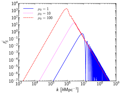
Figure 1: The kernel function $I_{S}^{j}$ defined in Eq. (37) for different macro model magnifications, $\mu_{0}=\mu_{j,1}\mu_{j,2}=1$ (solid), $10$ (dotted), and $100$ (dashed), which are computed changing $\mu_{j,1}$ while fixing $\mu_{j,2}=1$. They are computed assuming the lens redshift $z=0.3$, the source redshift $z_{\rm s}=2$, and the frequency of gravitational waves $f=10$ Hz, for which the inverse of the Fresnel scale is $1/r_{\rm F}\simeq 3\times 10^{6}h{\rm Mpc}^{-1}$.

III Discussions

III.1 Behavior of kernel functions

In Sec. II we show that dispersions of amplitude and phase shifts for strongly lensed, magnified gravitational waves are written by integrations of the convergence power spectra with kernel functions $I_{K}^{j}$ and $I_{S}^{j}$, respectively.

As was discussed in previous work [5, 8], when the macro model magnification is not considered, $\mu_{j,1}=\mu_{j,2}=1$, kernel functions peak at around $k\sim 1/r_{\rm F}$, which is evident from the fact that kernel functions are described as a function of $r_{\rm F}^{2}k^{2}$. Adopting $I_{S}^{j}$ defined in Eq. (37) as a specific example, we check how the kernel function is modified for highly magnified gravitational waves. Fig. 1 shows kernel functions $I_{S}^{j}$ for three different macro model magnifications $\mu_{0}=\mu_{j,1}\mu_{j,2}$. We find that the macro model magnification $\mu_{0}$ shifts the peak of the kernel function such that the effective Fresnel scale becomes larger in the presence of the macro model magnification. More importantly, we find that the overall amplitude of the kernel function is significantly boosted by the macro model magnification. The boosted amplitude and phase fluctuations can be explained by the nonlinear dependence of convergence perturbations on magnification factors [31]. We confirm that the similar dependence on $\mu_{0}$ is seen for the kernel function for the amplitude, $I_{K}^{j}$.

Since effects of small-scale perturbations on highly magnified images sometimes exhibit strong dependence on the image type i.e., whether the image originates from a local minimum (Type I), a saddle point (Type II), or a local maximum (Type III) of the arrival time surface (e.g. [32]), it is worth commenting on the possible image type dependence of our result. We emphasize that the equations derived in this paper do not rely on any assumption on the image type, and hence are applicable to all image types. We check the kernel functions for different image types to find that their dependence on the image type is weak. For instance, when $|\mu_{j,1}|\gg\mu_{j,2}>0$, kernel functions for positive $\mu_{\j,1}$ and negative $\mu_{\j,1}$ are almost indistinguishable with each other. The weak dependence on the image type is presumably because we consider the situation that perturbations do not create extra image pairs. In addition, our calculations are limited to the linear order in the density perturbation, while the strong image type dependence as mentioned above originates from the nonlinear dependence of the magnification on convergence and shear. This means that our calculation is valid only in the low frequency limit where contributions from individual perturbers are significantly suppressed due to the diffraction effect. We also note that effects of perturbations on Type II images may exhibit complex behaviors in the time domain as is the case for unperturbed images (e.g., [26, 29]). We leave for future work more thorough studies of the dependence of the perturbative wave optics effects on the image type.

We note that the dependence of the effective Fresnel scale and the peak height of the kernel functions can be estimated analytically. For the case of $I_{S}^{j}$ shown in Fig. 1, we find that, when $|\mu_{1}|\gg|\mu_{2}|$, the effective Fresnel scale depends on the macro model magnification as $\propto|\mu_{0}|^{1/2}$ and the peak of the kernel function as $\propto|\mu_{0}|^{2}$. On the other hand, when $\mu_{1}=\mu_{2}$ they exhibit different dependence on $\mu_{0}$ such that the effective Fresnel scale behaves as $\propto|\mu_{0}|^{1/4}$ and the peak of the kernel function as $\propto|\mu_{0}|$.

III.2 Dark matter substructure

In [8], it was concluded that amplitude and phase fluctuations due to dark matter substructures can be detected, if many observations of gravitational waves from compact binary mergers are combined statistically. Given the significant boost by the macro model magnification $\mu_{0}$, amplitude and phase fluctuations may be detected more easily for highly magnified gravitational waves, even for a small number of events. However, as discussed in [8], an obstacle is microlensing by stars in lensing galaxies or clusters of galaxies, which dominate at very small scales.

We consider a simple model of dark matter substructure to make a rough estimate of its detectability. The small-scale power spectrum at around the Einstein radius $r_{\rm Ein}$, where strongly lensed images typically appear, due to dark matter substructure can be modeled as (e.g., [33])

$$P_{\kappa}(k)=\int dm\frac{dn}{dm}\left(\frac{m}{\Sigma_{\rm cr}}\right)^{2}\left|\tilde{y}(k)\right|^{2},$$ (46)

where $\tilde{y}(k)$ is the Fourier transform of the normalized Navarro-Frenk-White (NFW) density profile [34], $\Sigma_{\rm cr}$ is the critical surface density in comoving units, and $dn/dm$ is the subhalo surface number density as a function of the subhalo mass $m$ at around the Einstein radius $r_{\rm Ein}$

$$\frac{dn}{dm}=p(r_{\rm Ein})\frac{dN}{dm},$$ (47)

with $p(r_{\rm Ein})=\Sigma_{\rm DM}(r_{\rm Ein})/M$ being the normalized dark matter density in the projected space for the host halo with mass $M$. We assume that the subhalo mass function $dN/dm$ follows a power-law shape

$$\frac{dN}{dm}=f_{\rm sub}\frac{2-\alpha}{f_{\rm cut}^{2-\alpha}}\left(\frac{m}{M}\right)^{-\alpha}\frac{1}{M}\;\;\;\;\;(m\leq f_{\rm cut}M).$$ (48)

This expression ensures that the overall mass fraction of subhalos reduces to $f_{\rm sub}$

$$\int_{0}^{f_{\rm cut}M}m\frac{dN}{dm}dm=f_{\rm sub}M.$$ (49)

We adopt the slope $\alpha=1.9$, the cutoff of the subhalo mass function $f_{\rm cut}=0.1$, and the overall mass fraction of subhalos $f_{\rm sub}=0.1$, as typical values of these parameters (e.g., [35]).

We also follow [8] to model the effect of stellar microlensing by the shot noise power spectrum due to the discrete nature of stars

$$P_{\kappa,{\rm shot}}(k)=f_{*}^{2}\frac{M_{*}}{f_{*}\Sigma(r_{\rm Ein})}\left\{\kappa(r_{\rm Ein})\right\}^{2}=\frac{f_{*}M_{*}\kappa(r_{\rm Ein})}{\Sigma_{\rm cr}},$$ (50)

where $f_{*}$ is the stellar mass fraction to the total mass density at the Einstein radius, $M_{*}$ is the mass of individual stars (i.e., we ignore the mass spectrum for simplicity), $\kappa(r_{\rm Ein})$ is the convergence value (the sum of dark matter and stellar component) of the main halo at the Einstein radius. This treatment of microlensing is expected to be valid when the Fresnel scale is larger than the Einstein radii of individual stars [8].

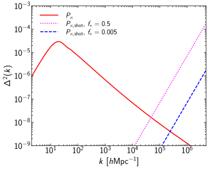
Figure 2: The small-scale dimensionless power spectra $\Delta^{2}(k)=k^{2}P(k)/(2\pi)$ at around the Einstein radius due to dark matter substructure $P_{\kappa}(k)$, Eq. (46), and microlensing by stars $P_{\kappa,{\rm shot}}(k)$, Eq. (50). See the text for parameters used for the calculation. For microlensing, we consider two cases with the stellar mass fraction of $f_{*}=0.5$ and $0.005$.

As a specific example, we compute the convergence power spectra adopting the host halo mass of $10^{13}h^{-1}M_{\odot}$ defined for the critical overdensity of $200$, the concentration parameter of $c=10$, the lens redshift of $z=0.3$, the source redshift of $z_{\rm s}=2$, the Einstein radius of $r_{\rm Ein}=0.03~{}r_{200}$, $\kappa(r_{\rm Ein})=0.5$, and $M_{*}=0.5~{}M_{\odot}$. We consider the stellar mass fraction at around the Einstein radius of both $f_{*}=0.5$ and $f_{*}=0.005$. The former is a typical value for galaxy-galaxy strong lens systems, while the latter may be achieved for strong lensing due to massive clusters of galaxies [36]. Fig. 2 shows the convergence power spectra from dark matter substructure, Eq. (46), as well as those from microlensing, Eq. (50). An example of convergence power spectra shown in Fig. 2 indicates that the effect of microlensing is dominated at the smaller scale, or equivalently the higher wavenumber $k$. Since the macro model magnification shifts the peak of the kernel function to the smaller $k$, it can significantly reduce the relative contribution of microlensing by stars to amplitude and phase fluctuations compared with that of dark matter substructure.

Figure 3: Phase dispersions as a function of the macro model magnification $\mu_{0}$ computed by Eq. (36) with convergence power spectra of dark matter substructure $P_{\kappa}(k)$, Eq. (46), and microlensing by stars $P_{\kappa,{\rm shot}}(k)$, Eq. (50), as shown in Fig. 2. The frequency of gravitational waves of $f=10$ Hz is adopted.

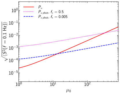
Figure 4: Similar to Fig. 3, but for $f=0.1$ Hz.

Fig. 3 shows phase dispersions as a function of the macro model magnification $\mu_{0}$ computed by Eq. (36) for the frequency of $f=10$ Hz that roughly corresponds to the low frequency end of ongoing ground based laser interferometers. In what follows, we change $\mu_{0}$ by changing $\mu_{j,1}$ while fixing $\mu_{j,2}=1$ such that $\mu_{0}=\mu_{j,1}\mu_{j,2}=\mu_{j,1}$, as done in Fig. 1. Since the dimensionless power spectrum due to dark matter substructure is a decreasing function of the wavenumber $k$, the phase dispersion is quite sensitive to the macro model magnification $\mu_{0}$. In contrast, the increase of the peak of the kernel function is somewhat compensated by the shift of the peak for the case of microlensing by stars, leading to the weaker dependence on $\mu_{0}$. Therefore, as expected, the macro model magnification $\mu_{0}$ not only increases the dispersion but also increases the relative contribution of dark matter substructure to microlensing, although the contribution of dark matter substructure appears to be subdominant even for very high $\mu_{0}$ at least within the parameter range we examined.

Since the effect of microlensing is more pronounced at the higher wavenumber $k$, it is expected that we can probe dark matter substructure more easily at lower frequency $f$. This point is clear from Fig. 4 in which results for $f=0.1$ Hz, which can be observed by space based laser interferometers, are shown. In this case, the contribution of dark matter substructure can become dominant, if the macro model magnification is sufficiently large and the stellar mass fraction is reasonably small. When the macro model magnification is sufficiently large, several hundreds, the typical phase shift can reach on the order of $0.1-0.01$, which can be detected from a single event if the signal-to-noise ratio of the observation is sufficiently high. We note that the expected magnification of strong lensing events detected by e.g., advanced LIGO, advanced VIRGO, and KAGRA tends to be high due to a strong selection effect [13], suggesting that such high magnification events may not be rare.

Our analysis indicates that microlensing by stars can induce non-negligible amplitude and phase shifts of highly magnified, multiply imaged gravitational waves. Such shifts, if significant, might degrade the performance of searching for multiple image pairs of gravitational wave events based on the similarly of waveform shapes. This effect might also degrade the application of using gravitational waves to constrain modified dispersion relations [37, 38, 39].

III.3 Fuzzy dark matter and primordial black holes

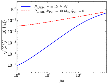
Figure 5: Phase dispersions as a function of the macro model magnification $\mu_{0}$ in the FDM (solid) and PBH (dashed) models for the frequency of $f=10$ Hz. The calculation in the FDM model is done using the convergence power spectrum shown in Eq. (51) with the FDM mass of $10^{-20}$eV, while that in the PBH model is based on the convergence power spectrum shown in Eq. (53) with $f_{\rm PBH}=0.1$ and $M_{\rm PBH}=30~{}M_{\odot}$. Here we assume the stellar mass fraction of $f_{*}=0.5$, and the other parameters are same as those used in Sec. III.2.

The small-scale matter power spectrum can test various dark matter models. For instance, Kawai et al. [40] proposed an analytic model of the small-small matter power spectrum in the Fuzzy Dark Matter (FDM) model. In this model the convergence power spectrum is given by

$$P_{\kappa,{\rm FDM}}(k)= (1-f_{*})^{2}\left\{\kappa(r_{\rm Ein})\right\}^{2}\frac{4\pi\lambda_{\rm c}^{3}}{3r_{\rm h}(r_{\rm Ein})}$$

$$\times\exp\left(-\frac{\lambda_{\rm c}^{2}k^{2}}{4}\right),$$ (51)

where $\lambda_{\rm c}$ is the de Broglie wavelength that is computed from the virial velocity of the host halo and $r_{\rm h}$ denotes an effective size of the halo defined by

$$r_{\rm h}(r_{\rm Ein})=\frac{\Sigma_{\rm DM}^{2}(r_{\rm Ein})}{\int dz\,\rho_{\rm DM}^{2}(\sqrt{r_{\rm Ein}^{2}+z^{2}})}.$$ (52)

Since in this paper the Fresnel scale and the wavenumber are defined in the comoving coordinate, we compute the quantities used above also in the comoving coordinate.

In addition, Oguri and Takahashi [8] discussed how the small-scale matter power spectrum is modified in the Primordial Black Hole (PBH) scenario. Here we ignore the enhancement of the halo formation due to the isocurvature perturbation, which turns out to be a relatively minor effect, and consider the shot noise due to the discrete nature of PBHs

$$P_{\kappa,{\rm PBH}}(k)=\frac{f_{\rm PBH}(1-f_{*})M_{\rm PBH}\kappa(r_{\rm Ein})}{\Sigma_{\rm cr}},$$ (53)

where $f_{\rm PBH}$ and $M_{\rm PBH}$ denote the relative abundance of PBHs with respect to the total dark matter density and the mass of each PBH, respectively.

Fig. 5 shows examples of phase fluctuations in the FDM and PBH models to demonstrate how they can give dominant contributions to the predicted phase fluctuations. In these examples the phase fluctuations become sufficiently large at high $\mu_{0}$ such that they dominate the contribution from stellar microlensing (see also [41] for more detailed studies on constraining PBHs with microlensing). This result indicates that amplitude and phase fluctuations of highly magnified gravitational waves may offer a powerful means of constraining dark matter models. We leave more detailed analysis on such applications to future work.

IV Summary

We have derived equations that connect the small-scale density perturbations on the Fresnel scale with amplitude and phase fluctuations of gravitational waves in the presence of macro model magnifications for which geometric optics is valid. We have found that amplitude and phase fluctuations due to perturbative wave optics effects are significantly boosted by macro model magnifications, which not only effectively increase the Fresnel scale but also increase the peak amplitudes of the kernel functions that are used to calculate the amplitude and phase fluctuations. We have found that amplitude and phase fluctuations due to dark matter substructure tend to be smaller than those from microlensing by stars, although the former could be detected for highly magnified gravitational waves in low frequencies, say $f=0.1$ Hz. We have also discussed amplitude and phase fluctuations in FDM and PBH models, and showed that they can produce large amplitude and phase fluctuations depending on model parameters. While in this paper we have focused on gravitational waves, the equations derived in this paper are not restricted to gravitational waves and can be applied to any sources. A caveat is that our results are based on linearized equations and hence ignore any nonlinear effects, although we expect that our formalism can be applied to a wide range of problems because the diffraction due to wave optics effects generally suppresses such nonlinear effects.

- [1] B. P. Abbott et al. [LIGO Scientific and Virgo], Phys. Rev. Lett. 116, no.6, 061102 (2016) doi:10.1103/PhysRevLett.116.061102 [arXiv:1602.03837 [gr-qc]].
- [2] T. T. Nakamura and S. Deguchi, Prog. Theor. Phys. Suppl. 133, 137 (1999) doi:10.1143/PTPS.133.137
- [3] M. Oguri, Rept. Prog. Phys. 82, no.12, 126901 (2019) doi:10.1088/1361-6633/ab4fc5 [arXiv:1907.06830 [astro-ph.CO]].
- [4] J. P. Macquart, Astron. Astrophys. 422, 761-775 (2004) doi:10.1051/0004-6361:20034512 [arXiv:astro-ph/0402661 [astro-ph]].
- [5] R. Takahashi, Astrophys. J. 644, 80-85 (2006) doi:10.1086/503323 [arXiv:astro-ph/0511517 [astro-ph]].
- [6] T. T. Nakamura, Phys. Rev. Lett. 80 (1998), 1138-1141 doi:10.1103/PhysRevLett.80.1138
- [7] R. Takahashi, T. Suyama and S. Michikoshi, Astron. Astrophys. 438, L5 (2005) doi:10.1051/0004-6361:200500140 [arXiv:astro-ph/0503343 [astro-ph]].
- [8] M. Oguri and R. Takahashi, Astrophys. J. 901, no.1, 58 (2020) doi:10.3847/1538-4357/abafab [arXiv:2007.01936 [astro-ph.CO]].
- [9] M. Inamori and T. Suyama, Astrophys. J. Lett. 918, no.2, L30 (2021) doi:10.3847/2041-8213/ac2142 [arXiv:2107.02443 [gr-qc]].
- [10] K. K. Y. Ng, K. W. K. Wong, T. Broadhurst and T. G. F. Li, Phys. Rev. D 97, no.2, 023012 (2018) doi:10.1103/PhysRevD.97.023012 [arXiv:1703.06319 [astro-ph.CO]].
- [11] T. Broadhurst, J. M. Diego and G. Smoot, [arXiv:1802.05273 [astro-ph.CO]].
- [12] S. S. Li, S. Mao, Y. Zhao and Y. Lu, Mon. Not. Roy. Astron. Soc. 476, no.2, 2220-2229 (2018) doi:10.1093/mnras/sty411 [arXiv:1802.05089 [astro-ph.CO]].
- [13] M. Oguri, Mon. Not. Roy. Astron. Soc. 480, no.3, 3842-3855 (2018) doi:10.1093/mnras/sty2145 [arXiv:1807.02584 [astro-ph.CO]].
- [14] G. Cusin, R. Durrer and I. Dvorkin, [arXiv:1912.11916 [astro-ph.CO]].
- [15] S. Mukherjee, T. Broadhurst, J. M. Diego, J. Silk and G. F. Smoot, Mon. Not. Roy. Astron. Soc. 501 (2021) no.2, 2451-2466 doi:10.1093/mnras/staa3813 [arXiv:2006.03064 [astro-ph.CO]].
- [16] R. Abbott et al. [LIGO Scientific and VIRGO], Astrophys. J. 923, no.1, 14 (2021) doi:10.3847/1538-4357/ac23db [arXiv:2105.06384 [gr-qc]].
- [17] J. M. Diego et al. [LIGO Scientific and VIRGO], Phys. Rev. D 104, no.10, 103529 (2021) doi:10.1103/PhysRevD.104.103529 [arXiv:2106.06545 [gr-qc]].
- [18] L. Yang, S. Wu, K. Liao, X. Ding, Z. You, Z. Cao, M. Biesiada and Z. H. Zhu, Mon. Not. Roy. Astron. Soc. 509, no.3, 3772-3778 (2021) doi:10.1093/mnras/stab3298 [arXiv:2105.07011 [astro-ph.GA]].
- [19] F. Xu, J. M. Ezquiaga and D. E. Holz, [arXiv:2105.14390 [astro-ph.CO]].
- [20] S. Mukherjee, T. Broadhurst, J. M. Diego, J. Silk and G. F. Smoot, Mon. Not. Roy. Astron. Soc. 506 (2021) no.3, 3751-3759 doi:10.1093/mnras/stab1980 [arXiv:2106.00392 [gr-qc]].
- [21] A. R. A. C. Wierda, E. Wempe, O. A. Hannuksela, L. é. V. E. Koopmans and C. Van Den Broeck, Astrophys. J. 921, no.2, 154 (2021) doi:10.3847/1538-4357/ac1bb4 [arXiv:2106.06303 [astro-ph.HE]].
- [22] J. M. Diego, O. A. Hannuksela, P. L. Kelly, T. Broadhurst, K. Kim, T. G. F. Li, G. F. Smoot and G. Pagano, Astron. Astrophys. 627, A130 (2019) doi:10.1051/0004-6361/201935490 [arXiv:1903.04513 [astro-ph.CO]].
- [23] M. H. Y. Cheung, J. Gais, O. A. Hannuksela and T. G. F. Li, Mon. Not. Roy. Astron. Soc. 503, no.3, 3326-3336 (2021) doi:10.1093/mnras/stab579 [arXiv:2012.07800 [astro-ph.HE]].
- [24] A. Mishra, A. K. Meena, A. More, S. Bose and J. S. Bagla, Mon. Not. Roy. Astron. Soc. 508, no.4, 4869-4886 (2021) doi:10.1093/mnras/stab2875 [arXiv:2102.03946 [astro-ph.CO]].
- [25] S. M. C. Yeung, M. H. Y. Cheung, J. A. J. Gais, O. A. Hannuksela and T. G. F. Li, [arXiv:2112.07635 [gr-qc]].
- [26] J. M. Ezquiaga, D. E. Holz, W. Hu, M. Lagos and R. M. Wald, Phys. Rev. D 103, no.6, 064047 (2021) doi:10.1103/PhysRevD.103.064047 [arXiv:2008.12814 [gr-qc]].
- [27] L. Dai, S. S. Li, B. Zackay, S. Mao and Y. Lu, Phys. Rev. D 98, no.10, 104029 (2018) doi:10.1103/PhysRevD.98.104029 [arXiv:1810.00003 [gr-qc]].
- [28] H. G. Choi, C. Park and S. Jung, Phys. Rev. D 104, no.6, 063001 (2021) doi:10.1103/PhysRevD.104.063001 [arXiv:2103.08618 [astro-ph.CO]].
- [29] L. Dai and T. Venumadhav, [arXiv:1702.04724 [gr-qc]].
- [30] L. Dai, B. Zackay, T. Venumadhav, J. Roulet and M. Zaldarriaga, [arXiv:2007.12709 [astro-ph.HE]].
- [31] S. d. Mao and P. Schneider, Mon. Not. Roy. Astron. Soc. 295, 587-594 (1998) doi:10.1046/j.1365-8711.1998.01319.x [arXiv:astro-ph/9707187 [astro-ph]].
- [32] P. L. Schechter and J. Wambsganss, Astrophys. J. 580 (2002), 685-695 doi:10.1086/343856 [arXiv:astro-ph/0204425 [astro-ph]].
- [33] Y. Hezaveh, N. Dalal, G. Holder, T. Kisner, M. Kuhlen and L. Perreault Levasseur, JCAP 11, 048 (2016) doi:10.1088/1475-7516/2016/11/048 [arXiv:1403.2720 [astro-ph.CO]].
- [34] J. F. Navarro, C. S. Frenk and S. D. M. White, Astrophys. J. 490, 493-508 (1997) doi:10.1086/304888 [arXiv:astro-ph/9611107 [astro-ph]].
- [35] V. Springel, J. Wang, M. Vogelsberger, A. Ludlow, A. Jenkins, A. Helmi, J. F. Navarro, C. S. Frenk and S. D. M. White, Mon. Not. Roy. Astron. Soc. 391, 1685-1711 (2008) doi:10.1111/j.1365-2966.2008.14066.x [arXiv:0809.0898 [astro-ph]].
- [36] P. L. Kelly, J. M. Diego, S. Rodney, N. Kaiser, T. Broadhurst, A. Zitrin, T. Treu, P. G. Pérez-González, T. Morishita and M. Jauzac, et al. Nature Astron. 2, no.4, 334-342 (2018) doi:10.1038/s41550-018-0430-3 [arXiv:1706.10279 [astro-ph.GA]].
- [37] C. M. Will, Phys. Rev. D 57 (1998), 2061-2068 doi:10.1103/PhysRevD.57.2061 [arXiv:gr-qc/9709011 [gr-qc]].
- [38] A. K. W. Chung and T. G. F. Li, Phys. Rev. D 104 (2021) no.12, 124060 doi:10.1103/PhysRevD.104.124060 [arXiv:2106.09630 [gr-qc]].
- [39] J. M. Ezquiaga, W. Hu, M. Lagos, M. X. Lin and F. Xu, [arXiv:2203.13252 [gr-qc]].
- [40] H. Kawai, M. Oguri, A. Amruth, T. Broadhurst and J. Lim, Astrophys. J. 925, no.1, 61 (2022) doi:10.3847/1538-4357/ac39a2 [arXiv:2109.04704 [astro-ph.CO]].
- [41] J. M. Diego, Phys. Rev. D 101, no.12, 123512 (2020) doi:10.1103/PhysRevD.101.123512 [arXiv:1911.05736 [astro-ph.CO]].