LoCoV: low dimension covariance voting algorithm for portfolio optimization

Abstract

Minimum-variance portfolio optimizations rely on accurate covariance estimator to obtain optimal portfolios. However, it usually suffers from large error from sample covariance matrix when the sample size $n$ is not significantly larger than the number of assets $p$. We analyze the random matrix aspects of portfolio optimization and identify the order of errors in sample optimal portfolio weight and show portfolio risk are underestimated when using samples. We also provide LoCoV (low dimension covariance voting) algorithm to reduce error inherited from random samples. From various experiments, LoCoV is shown to outperform the classical method by a large margin.

1 Introduction

Portfolio theory pioneered by Markowitz in 1950’s [9] is at the center of theoretical developments in finance. The mean-variance model tells investors should hold a portfolio on the efficient frontier which trade off portfolio mean (return) against variance (risk). In practice, mean and variance are calculated using estimated sample mean and sample covariance matrix. However, estimation error in sample mean and covariance will significantly affect the accuracy of the portfolio thus perform poorly in practice (see [7, 10]). Quantitative result on how sample covariance affects the performance are very limited. The bias in sample portfolio weight is discussed in [5] but no practical guidance is given on how large is the bias when use mean-variance model with sample data. We in this work will obtain that the order of magnitude of the error in sample portfolio weight which is large when the sample size $n$ is comparable to the number of assets $p$. And the error decays in the rate of $\sqrt{\frac{p}{n}}$ as $n$ increases.

For this reason, there has been many work suggest different approaches to overcome standard mean-variance portfolio optimizations. These suggestions include imposing portfolio constraints (see [6, 3, 1]), use of factor models ([2]), modifying objective to be more robust ([4]) and improving sample covariance matrix estimation ([8]). Instead, in this work we use the observation from random matrix theory to provide alternative view on the error in sample covariance matrix. We propose LoCoV, low dimension covariance voting, which effectively exploits the accurate low dimensional covariance to vote on different assets. It outperform the standard sample portfolio by a large margin.

We shall first set up the problem. For simplicity, we only discuss minimum-variance portfolio optimization. Assume the true covariance admits diagonalization

$$\Sigma=P^{T}D^{2}P$$

where $D$ is a non-negative definite diagonal matrix, and $P$ is an orthogonal matrix. Then a data matrix (asset return) realized by random matrix ${\mathcal{N}}(n\times p)$ with i.i.d. standard random variables is

$$X={\mathcal{N}}DP$$

a sample covariance matrix is then obtained as

$$\hat{\Sigma}=P^{T}D\frac{{\mathcal{N}}^{T}{\mathcal{N}}}{n}DP$$

We define the minimum variance portfolio to be the optimizer of

$$\begin{split}\min_{w}\;&w^{T}\Sigma\;w\\ s.t.\;&w^{T}\mathbbm{1}=1\end{split}$$ (1.1)

where $\mathbbm{1}=\left[\begin{array}[]{ccc}1&\cdots&1\\ \end{array}\right]^{T}$. In reality, $\Sigma$ is not known, therefore it is replaced by an estimator $\hat{\Sigma}$ to obtain an approximated optimal portfolio. That is we solve

$$\begin{split}\min_{w}\;&w^{T}\hat{\Sigma}\;w\\ s.t.\;&w^{T}\mathbbm{1}=1\end{split}$$ (1.2)

2 Universality of optimal portfolio weight and risk

We first derive the solution of minimum-variance by the method of Lagrange multiplier since a closed form is available. Later on based on the explicit form of the solutions, we will investigate probabilistic properties of portfolio weight and risk.

Observe that both $\Sigma$ and $\hat{\Sigma}$ take the form $A^{T}A$ where $A$ is $DP$ for true covariance $\Sigma$ and $A$ is $\frac{1}{\sqrt{n}}{\mathcal{N}}DP$ for the sample covariance matrix $\hat{\Sigma}$. We shall define the portfolio optimization in the general form

$$\begin{split}\min_{w}\;&w^{T}A^{T}A\;w\\ s.t.\;&w^{T}\mathbbm{1}=1\end{split}$$ (2.1)

Define the Lagrangian function

$${\mathcal{L}}(w)=w^{T}A^{T}Aw-\lambda(w^{T}\mathbbm{1}-1)$$

Taking derivatives with respect to the portfolio weight $w$, and set the gradient to be zero,

$$\nabla{\mathcal{L}}=2w^{T}A^{T}A-\lambda\mathbbm{1}^{T}=0$$

write gradient as column vector this is

$$2A^{T}Aw=\lambda\mathbbm{1}$$

For real life portfolio optimization, we can assume $A^{T}A$ ($\Sigma$ or $\hat{\Sigma}$) is invertible since otherwise optimal portfolio weight will have large error or ambiguity. Then we find the optimal portfolio weight

$$w=\frac{\lambda}{2}(A^{T}A)^{-1}\mathbbm{1}$$

We know the portfolio weights should be normalized so that they sum up to 1. Therefore $\lambda/2$ is essentially a normalizing factor. For convenience of notation, we make the following definition.

Definition 1.

The free (non-normalized) optimal weight of portfolio optimization 2.1 is

$$S=\left[\begin{array}[]{ccc}s_{1}&\cdots&s_{p}\\ \end{array}\right]^{T}=(A^{T}A)^{-1}\mathbbm{1}$$

And denote its sum as

$$\|S\|_{s}:=\sum_{k=1}^{p}s_{k}$$

Normalizing the vector $S$ we obtain optimal portfolio weight

$$w^{*}=\frac{1}{\sum_{i=1}^{p}s_{i}}S=\frac{S}{\|S\|_{s}}$$

It is easy to see $\lambda^{*}=\frac{2}{\sum_{i=1}^{p}s_{i}}=2\|S\|_{s}^{-1}$. Then take dot product of $\nabla{\mathcal{L}}$ and $w$, we find

$$0=\nabla{\mathcal{L}}^{T}w=2w^{T}A^{T}Aw-\lambda\mathbbm{1}^{T}w$$

and recall $\mathbbm{1}^{T}w=1$, therefore, we find the minimum portfolio risk

$$R(w^{*})=w^{*T}A^{T}Aw^{*}=\lambda^{*}/2=\|S\|_{s}^{-1}$$

We summarize the result as follows,

Proposition 2.

For the constrained optimization 2.1, the free optimal weight is

$$S=\left[\begin{array}[]{c}s_{1}\\ \vdots\\ s_{p}\\ \end{array}\right]=(A^{T}A)^{-1}\mathbbm{1}$$ (2.2)

Normalizing $S$, we obtain the optimal portfolio weight

$$w^{*}=\|S\|_{s}^{-1}S$$ (2.3)

and the minimum portfolio risk is

$$R(w^{*})=\|S\|_{s}^{-1}$$ (2.4)

where $\|S\|_{s}^{-1}=\sum_{k=1}^{p}s_{k}$.

2.1 Behavior of sample portfolio

Assume the diagonalization of true covariance matrix

$$\Sigma=P^{T}D^{2}P=P^{T}diag(\sigma_{1}^{2},\cdots,\sigma_{p}^{2})P$$

By proposition 2, plugging in $A^{T}A=\Sigma$, we find the true free optimal weight and true optimal portfolio weight of 1.1 are

$$S_{\Sigma}=\Sigma^{-1}\mathbbm{1}=P^{T}D^{-2}P\mathbbm{1},\qquad w^{*}=\|S_{\Sigma}\|_{s}^{-1}S_{\Sigma}$$ (2.5)

Then recall the return (data matrix) is generated as $X={\mathcal{N}}DP$ where ${\mathcal{N}}$ is a $n\times p$ matrix with i.i.d. standard random variables (mean zero and variance one). This leads to the sample covariance matrix

$$\hat{\Sigma}=P^{T}D\frac{{\mathcal{N}}^{T}{\mathcal{N}}}{n}DP$$

Plugging in $A^{T}A=\hat{\Sigma}$ for proposition 2, we obtain sample free optimal weight and sample optimal portfolio weight of 1.2

$$S_{\hat{\Sigma}}=P^{T}\hat{\Sigma}^{-1}P\mathbbm{1}=P^{T}D^{-1}\left(\frac{{\mathcal{N}}^{T}{\mathcal{N}}}{n}\right)^{-1}D^{-1}P\mathbbm{1},\qquad\hat{w}^{*}=\|S_{\hat{\Sigma}}\|_{s}^{-1}S_{\hat{\Sigma}}$$ (2.6)

The difference between $S_{\hat{\Sigma}}$ and $S_{\Sigma}$ depends on the random matrix (inverse of sample covariance) $M:=\left(\frac{{\mathcal{N}}^{T}{\mathcal{N}}}{n}\right)^{-1}$, diagonal matrix $D$ and orthogonal matrix $P$. $M$ is the inverse of a sample covariance matrix. It is possible to directly use the formula for inverse from Cramer rule to analyze this random matrix and show $\operatorname{\mathbb{E}}M=I$. Since this work mainly focus on improving the accuracy of portfolio, we will not pursue the probabilistic properties here (which shall be discussed in another work elsewhere). Instead we use several experiments to show the sample portfolio weight $\hat{w}^{*}$ is centered around the true portfolio weight $w^{*}$.

2.2 First example: sample portfolio of independent assets

We shall start with the simplest case that all assets are independent, i.e. the matrix $P$ is identity. This means the true covariance matrix is a diagonal matrix $\Sigma=D^{2}$. Then by 2.5 true free optimal weight and true optimal portfolio weight

$$S_{\Sigma}=\Sigma^{-1}\mathbbm{1}=D^{-1}D^{-1}\mathbbm{1}=\left[\begin{array}[]{ccc}\sigma_{1}^{-2}&\cdots&\sigma_{p}^{-2}\\ \end{array}\right]^{T},\qquad w^{*}=\|S_{\Sigma}\|_{s}^{-1}S_{\Sigma}$$

Similarly by 2.6 sample free optimal weight and sample optimal portfolio weight

$$S_{\hat{\Sigma}}=\hat{\Sigma}^{-1}\mathbbm{1}=D^{-1}\left(\frac{{\mathcal{N}}^{T}{\mathcal{N}}}{n}\right)^{-1}D^{-1}\mathbbm{1},\qquad\hat{w}^{*}=\|S_{\hat{\Sigma}}\|_{s}^{-1}S_{\hat{\Sigma}}$$

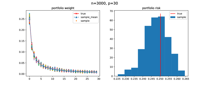
Figure 2: We select eigenvalues of $\Sigma$ equally spaced between 1 to 30. Namely $\sigma_{k}^{2}=k,1\leq k\leq 30$. We generate 300 samples for each of the two settings $(n,p)=(30,30)$ and $(3000,30)$. when $\frac{p}{n}=1$, the error of the portfolio weight is $O(1)$. when $\frac{p}{n}=1/100$, the error of the portfolio weight is $O(1/10)$

On the left figure 2, true optimal weight is red line which is closely aligned with the mean value of sample optimal weights which is show as blue connected dash-line. As we see the standard deviation in sample portfolio weight is at $O(\sqrt{p/n})$. As $p/n$ decreases, the sample portfolio weight become less volatile around the true portfolio weight. On the right, the sample optimal risk has higher chance of underestimate the true optimal risk. As $p/n$ decreases, the sample portfolio risk become less volatile and more centered around the true portfolio risk.

2.3 Second example: sample portfolio of dependent assets

For general assets with dependence, 2.5 and 2.6 have provided the formulas. Again we will only use experiments to show relations between the sample portfolio weight $\hat{w}^{*}$ and the true portfolio weight $w^{*}$.

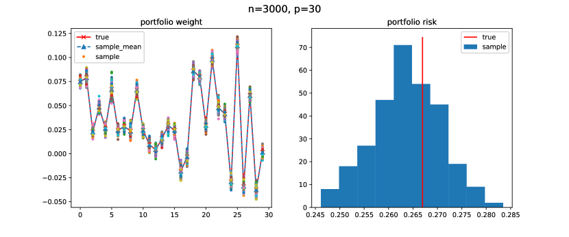
Figure 4: We still select eigenvalues of $\Sigma$ equally spaced between 1 to 30. Namely $\sigma_{k}^{2}=k,1\leq k\leq 30$. We now select $P$ to be a random orthogonal matrix according to the Haar measure.

Since we are using non-identity orthogonal matrix $P$ to create dependence among the assets, the true optimal portfolio weight is not ordered. The concentration and deviation properties of the sample portfolio weight has not changed. On the left figure 4, true optimal weight is the red line which is still closely aligned with the mean value of sample optimal weights which is shown as blue connected dash-line. As we see the standard deviation in sample portfolio weight is at $O(p/n)$. On the right, the sample optimal risk has higher chance of underestimate the true optimal risk. As $p/n$ decreases, both sample weight and sample risk become more accurate.

2.4 The order of error in sample optimal portfolio

We summarize our findings from previous examples and experiments as the following conjecture

Conjecture 1.

Error estimates for $\hat{w}^{*}$ (2.6) compared with $w^{*}$( 2.5): If assume eigenvalues of true covariance matrix $\Sigma$ are $\sigma_{k}^{2}$, then

$$\operatorname{\mathbb{E}}|\hat{w}^{*}_{k}-w^{*}_{k}|=O\left(\sigma_{k}\times\sqrt{\frac{p}{n}}\right),\quad\forall 1\leq k\leq n$$

The constant in the order depends on smallest and largest eigenvalues of $\Sigma$.

Even though we can not prove this in full generality, we can show

Theorem 2.

Assume the true covariance of assets has diagonalization $\Sigma=P^{T}D^{2}P$ with $D=diag(\sigma_{1},\cdots\sigma_{p})$ and asset return data $X={\mathcal{N}}DP$ where ${\mathcal{N}}$ is a $n\times p$ matrix with i.i.d. standard Gaussian random variables (mean zero and variance one). And the sample covariance matrix

$$\hat{\Sigma}=P^{T}D\frac{{\mathcal{N}}^{T}{\mathcal{N}}}{n}DP$$

Then error in sample free optimal weight $S_{\hat{\Sigma}}$ of 2.6 satisfies the bound

$$\operatorname{\mathbb{E}}\|S_{\hat{\Sigma}}-S_{{\Sigma}}\|_{2}\leq O\left(p\;\sigma_{max}\;\sigma_{min}^{-1}\sqrt{\frac{p}{n}}\right)$$

with high probability. where $\|\cdot\|$ is the matrix 2-norm.

Proof: From 2.5 and 2.6, we know the free optimal weights $S_{\Sigma}$ and $S_{\hat{\Sigma}}$ solves the linear system

$$\Sigma S_{\Sigma} =P^{T}D^{2}PS_{\Sigma}=\mathbbm{1}$$

$${\hat{\Sigma}}S_{\hat{\Sigma}} =P^{T}D\left(\frac{{\mathcal{N}}^{T}{\mathcal{N}}}{n}\right)DPS_{\hat{\Sigma}}=\mathbbm{1}$$

To compare $S_{\Sigma}$ and $S_{\hat{\Sigma}}$, we use perturbation theory of linear systems. Given linear system $Ax=b$ and its perturbed version $(A+B)\hat{x}=b$. then

$$(A+B)(\hat{x}-x+x) =b$$

$$(A+B)(\hat{x}-x) =Ax-(A+B)x$$

$$\hat{x}-x =-(A+B)^{-1}Bx$$

Therefore for any norm $\|\cdot\|$.

$$\|\hat{x}-x\|\leq\|(A+B)^{-1}B\|\|x\|$$

Replace $A=P^{T}D^{2}P$ and $A+B=P^{T}D\left(\frac{{\mathcal{N}}^{T}{\mathcal{N}}}{n}\right)DP$, we find

$$\|S_{\Sigma}-S_{\hat{\Sigma}}\|_{2} \leq\left\|P^{T}D^{-1}\left(\frac{{\mathcal{N}}^{T}{\mathcal{N}}}{n}\right)^{-1}D^{-1}PP^{T}D\left(\frac{{\mathcal{N}}^{T}{\mathcal{N}}}{n}-I\right)DP\right\|_{2}\|S_{\Sigma}\|_{2}$$

$$\leq\left\|P^{T}D^{-1}\left(\frac{{\mathcal{N}}^{T}{\mathcal{N}}}{n}\right)^{-1}\left(\frac{{\mathcal{N}}^{T}{\mathcal{N}}}{n}-I\right)DP\right\|_{2}\|S_{\Sigma}\|_{2}$$

Notice $D$ is diagonal and $P$ is orthogonal, we see

$$\|D\|_{2}=\sigma_{max},\;\|D^{-1}\|_{2}=\sigma_{min}^{-1},\;\|P\|_{2}=1$$

Denote $M:=\frac{{\mathcal{N}}^{T}{\mathcal{N}}}{n}$. Therefore we have the bound

$$\|S_{\Sigma}-S_{\hat{\Sigma}}\|_{2}\leq\|S_{\Sigma}\|_{2}\sigma_{min}^{-1}\sigma_{max}\left\|I-M^{-1}\right\|_{2}$$

Notice

$$\|I-M^{-1}\|_{2} =\max(|1-\lambda_{min}^{-1}|,|1-\lambda_{max}^{-1}|)$$

$$\leq|1-\lambda_{min}^{-1}|+|1-\lambda_{max}^{-1}|$$

$$=\lambda_{min}^{-1}-\lambda_{max}^{-1}$$

From random matrix theory, eigenvalues of $M$ follows Marchenko-Pastur distribution. Moreover, smallest and largest eigenvalues of $M$ satisfies (see [11])

$$\operatorname{\mathbb{E}}\lambda_{max}(M)\leq\left(1+\sqrt{\frac{p}{n}}\right)^{2},\;\operatorname{\mathbb{E}}\lambda_{min}(M)\geq\left(1-\sqrt{\frac{p}{n}}\right)^{2}$$

It is known the non-asymptotic behavior of $\lambda_{max}$ and $\lambda_{min}$ satisfies sub-exponential tails

$$\mathbb{P}\left(\left(1-\sqrt{\frac{p}{n}}\right)^{2}-t\leq\lambda_{min}(M)\leq\lambda_{max}(M)\leq\left(1+\sqrt{\frac{p}{n}}\right)^{2}+t\right)\leq 2e^{-\sqrt{n}t}$$

The sub-exponential tail properties implies with high probability ($1-O(n^{-c})$) so that $\lambda_{min}\geq 1-O(\sqrt{\frac{p}{n}})$ and $\lambda_{max}\leq 1+O(\sqrt{\frac{p}{n}})$ is concentrated around $(\operatorname{\mathbb{E}}\lambda_{min})^{-1}-(\operatorname{\mathbb{E}}\lambda_{max})^{-1}$. Then with high probability

$$\operatorname{\mathbb{E}}\|I-M^{-1}\|_{2} \leq\operatorname{\mathbb{E}}\lambda_{min}^{-1}-\operatorname{\mathbb{E}}\lambda_{max}^{-1}$$

$$\leq C\left[\frac{1}{1-O(\sqrt{\frac{p}{n}})}-\frac{1}{1+O(\sqrt{\frac{p}{n}})}\right]$$

$$=O(\sqrt{\frac{p}{n}})$$

Therefore we conclude

$$\|S_{\Sigma}-S_{\hat{\Sigma}}\|_{2}\leq\|S_{\Sigma}\|_{2}\;\sigma_{min}^{-1}\sigma_{max}O(\sqrt{\frac{p}{n}})$$

∎

Notice this result is closely related to how $\hat{w}^{*}$ behave. For instance, if we assume $D=P=I$, then $\|S_{\Sigma}\|_{2}=p$, we see

$$\|w^{*}-\hat{w}^{*}\|_{2}\leq\|\hat{w}^{*}-S_{\hat{\Sigma}}/p\|_{2}+\sigma_{min}^{-1}\sigma_{max}O(\sqrt{\frac{p}{n}})$$

3 LoCoV: low dimension covariance voting

So far we have seen that large errors are present when we use 1.2 to approximate 1.1 especially when $p/n$ is not small. The natural question is whether there is a rescue to reduce the errors when $p$ and $n$ are comparable. The answer is positive and we provide LoCoV algorithm, low dimension covariance voting, which consistently outperform the sample optimal portfolio $\hat{w}^{*}$.

Let us start with the motivation behind LoCoV. From random matrix theory, the sample covariance approaches to the true covariance as $p/n\to 0$. Suppose we have $n=30$ samples for $p=30$ assets. Then for any two assets, $X_{k}$ and $X_{t}$, the $2\times 2$ sample covariance matrix $\hat{\Sigma}_{ks}$ for assets $X_{k}$ and $X_{t}$ has 30 samples thus feature-to-sample ratio is $2/30$ which is much smaller compared with $30/30$ for the sample covariance matrix $\hat{\Sigma}$ for all 30 assets.

On the other hand, philosophically portfolio optimization is to compare different assets and find proper investment hedges (ratios). Since we have a very accurate sample covariance matrix $\hat{\Sigma}_{kt}$ for asset $X_{k}$ and $X_{t}$, we can find accurate investment relative-weights ($u_{k},u_{t}$), invest $u_{k}$ on asset $X_{k}$ and $u_{t}$ on asset $X_{t}$, by solving 1.2. As we repeat this process for any pair of two assets, we can use these low dimension covariance matrices $\hat{\Sigma}_{kt}$ to accurately construct ratios $(u_{k},u_{t})$ and then we utilize all $p^{2}$ pairs of ratios to vote on each assets and obtain a final portfolio weight vector.

1

Data: centered asset return $X\in\mathbb{R}^{n\times p}$, $n,p>0$

2 Compute sample covariance matrix $\hat{\Sigma}\leftarrow\frac{1}{n}X^{T}X$

3Initialization: $U\leftarrow\frac{1}{2}I$, $V\leftarrow 0$.

  // $U$ is $p\times p$ relative-weight matrix, $V$ is $p\times 1$ free-weight vector

4

5for $i\leftarrow 1$ to $p$ do

       /* 1. For asset $i$ find relative-weights */

6       for $j\leftarrow i+1$ to $p$ do

7             Extract $2\times 2$ sub-matrix $\hat{\Sigma}_{i,j}$, and solve the 2-assets portfolio optimization

$$\begin{split}&\min_{u}\;u^{T}\hat{\Sigma}_{i,j}\;u\\ &s.t.\;u^{T}\mathbbm{1}=1\end{split}$$

or use formula $u=(u_{1},u_{2})=\hat{\Sigma}_{i,j}^{-1}\mathbbm{1}$.

            $U_{i,j}\leftarrow u_{1}$

              // invest $u_{1}$ in asset $i$

8            

            $U_{j,i}\leftarrow u_{2}$

              // invest $u_{2}$ in asset $j$

9            

10       end for

11      

      /* 2. Voting */

12       Compute free-weight by uniform voting

$$V_{i}\leftarrow\frac{1}{p}\sum_{j=1}^{p}U_{i,j}$$

13 end for

14

15Normalize $V$

$$w\leftarrow\frac{V}{\|V\|_{s}}=\frac{V}{\sum_{i=1}^{p}V_{i}}$$

Output: $w$

Algorithm 1 ‘LoCoV-$2$’

And we can easily generalize this algorithm to that using $k\times k$ dimensional covariance and solve corresponding 1.2 for $k$ assets instead of using $2\times 2$ low dimensional covariance. Therefore we propose the following ‘LoCoV-$k$’ algorithm.

1

Data: centered asset return $X\in\mathbb{R}^{n\times p}$, $n,p>0$

2 Compute sample covariance matrix $\hat{\Sigma}\leftarrow\frac{1}{n}X^{T}X$

3Initialization: $U\leftarrow\frac{1}{k}\mathbbm{1}\mathbbm{1}^{T}$, $V\leftarrow 0$.

  // $\mathbbm{1}$ is $p\times 1$ vector of all ones, $V$ is $p\times 1$ free-weight vector

4

5for $i\leftarrow 1$ to $p$ do

       /* 1. For asset $i$ find relative-weights */

6       for $j\leftarrow 1$ to $p$ do

7             Generate index set $I=\{i,l_{1},\cdots,l_{k-1}\}$ where $l_{1},\cdots l_{k-1}$ random uniformly in $\{1,\cdots,p\}\setminus\{i\}$.

8            Extract $k\times k$ sub-matrix $\hat{\Sigma}_{I}$, and solve the k-assets portfolio optimization

$$\begin{split}&\min_{u}\;u^{T}\hat{\Sigma}_{I}\;u\\ &s.t.\;u^{T}\mathbbm{1}=1\end{split}$$

or use formula $u=(u_{0},u_{1},\cdots,u_{k-1})=\hat{\Sigma}_{I}^{-1}\mathbbm{1}$.

            $U_{i,j}\leftarrow\frac{1}{2}u_{0}+\frac{1}{2}U_{i,j}$

              // invest $u_{0}$ in asset $i$

9            

            $U_{l_{t},i}\leftarrow\frac{1}{2}u_{t}+\frac{1}{2}U_{l_{t},i},\quad\forall 1\leq t\leq k-1$

              // invest $u_{t}$ in asset $l_{t}$

10            

11       end for

12      

      /* 2. Voting */

13       Compute free-weight by uniform voting

$$V_{i}\leftarrow\frac{1}{p}\sum_{j=1}^{p}U_{i,j}$$

14 end for

15

16Normalize $V$

$$w\leftarrow\frac{V}{\|V\|_{s}}=\frac{V}{\sum_{i=1}^{p}V_{i}}$$

Output: $w$

Algorithm 2 ‘LoCoV-$k$’ ($k\geq 3$)

In LoCoV-$k$, there are several tweaks from LoCoV-$2$ in order to adapt to $k$-assets. Every time we solve a $k$-assets portfolio optimization problem, we obtain $k$ relative weights. In order to use all $k$ weights, we initialize the relative-weight matrix $U$ with all entries being $\frac{1}{k}$. If there is a new weight generated from the computation, we take average of the existing weight and the new weight. This update will diminish old weights which is only for convenience reading and understanding the algorithm. One could take a more delicate update on entries of $U$, for example keep track of the total number of weights generated for each entry, and then update with an average of all weights.

4 Simulations

We run three experiments and select $\Sigma=I,D^{2},P^{T}D^{2}P$. For each experiment, we generate 300 samples $\hat{\Sigma}$ and compute corresponding $\hat{w}^{*}$ and LoCoV estimator. We plot $\hat{w}^{*}$ in green and LoCoV-weight in black. The experiments show LoCoV consistently outperforms the sample optimal portfolio.

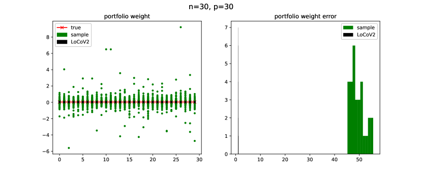
Figure 5: $\Sigma=I$

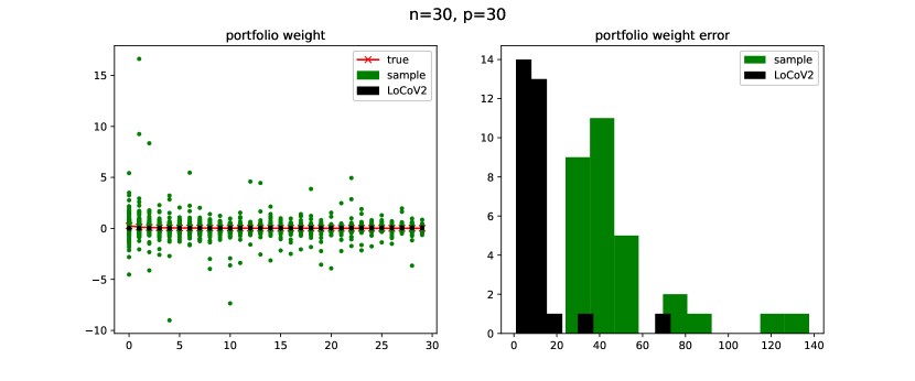
Figure 6: $\Sigma=D^{2}$ with eigenvalues of $\Sigma$ equally spaced between 1 to 30. Namely $\sigma_{k}^{2}=k,1\leq k\leq 30$.

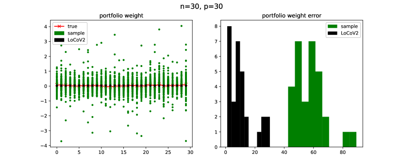
Figure 7: $\Sigma=P^{T}D^{2}P$ with eigenvalues of $\Sigma$ equally spaced between 1 to 30. Namely $\sigma_{k}^{2}=k,1\leq k\leq 30$. $P$ is a random orthogonal matrix according to the Haar measure.

5 Conclusion and open question

We analyzed the minimum variance portfolio question with the consideration of randomness of sample covariance matrix. In light of random matrix theory, we use experiments showed the error in sample optimal portfolio has the order of the assets-to-sample ratio $p/n$. When number of assets $p$ is not considerably smaller than the number of samples $n$, the sample optimal portfolio fails to provide accurate estimation of true optimal portfolio. Thus we proposed the LoCoV method which exploits the fact that $k$-dimensional sub-covariance matrix is more accurate thus can be used to produce relative weights among $k$ assets. Using relative weights to uniformly vote on given assets eventually improve dramatically on the performance of the portfolio.

5.1 Adapt LoCoV to general mean-variance portfolio

We have not discussed the role of mean return and assumed our data is centered. To adapt to general non-centered mean-variance portfolio optimization, one must modify the $k$-assets optimization sub-problem. Namely, one has to compute sample mean $\mu=\frac{1}{n}X_{i\cdot}$, and then solve the k-assets portfolio optimization

$$\begin{split}\min_{u}\;&u^{T}\hat{\Sigma}_{I}\;u\\ s.t.\;&u^{T}\mathbbm{1}=1\\ &\mu u\geq r_{0}\end{split}$$

where $r_{0}$ is the lower bound of expected return.

However, there is no guarantee to achieve the mean return $\mu w\geq r_{0}$ for the voting procedure produced weight $w$. Of course one can try to apply LoCoV first and check whether mean return is above the threshold $r_{0}$, if not then repeating the process of updating relative-weight matrix $U$ will probably improve.

References

[1]
Patrick Behr, Andre Guettler, and Felix Miebs.
On portfolio optimization: Imposing the right constraints.
Journal of Banking & Finance, 37(4):1232–1242, 2013.
[2]
Louis KC Chan, Jason Karceski, and Josef Lakonishok.
On portfolio optimization: Forecasting covariances and choosing the
risk model.
The review of Financial studies, 12(5):937–974, 1999.
[3]
Victor DeMiguel, Lorenzo Garlappi, Francisco J Nogales, and Raman Uppal.
A generalized approach to portfolio optimization: Improving
performance by constraining portfolio norms.
Management science, 55(5):798–812, 2009.
[4]
Victor DeMiguel and Francisco J Nogales.
Portfolio selection with robust estimation.
Operations Research, 57(3):560–577, 2009.
[5]
Noureddine El Karoui.
High-dimensionality effects in the markowitz problem and other
quadratic programs with linear constraints: Risk underestimation.
The Annals of Statistics, 38(6):3487–3566, 2010.
[6]
Ravi Jagannathan and Tongshu Ma.
Risk reduction in large portfolios: Why imposing the wrong
constraints helps.
The Journal of Finance, 58(4):1651–1683, 2003.
[7]
J David Jobson and Robert M Korkie.
Putting markowitz theory to work.
The Journal of Portfolio Management, 7(4):70–74, 1981.
[8]
Olivier Ledoit and Michael Wolf.
Improved estimation of the covariance matrix of stock returns with an
application to portfolio selection.
Journal of empirical finance, 10(5):603–621, 2003.
[9]
Harry M Markowitz.
Portfolio selection.
Journal of Finance, 7(1):77–91, 1952.
[10]
Richard O Michaud.
The markowitz optimization enigma: Is ‘optimized’optimal?
Financial analysts journal, 45(1):31–42, 1989.
[11]
Mark Rudelson and Roman Vershynin.
Non-asymptotic theory of random matrices: extreme singular values.
In Proceedings of the International Congress of Mathematicians
2010 (ICM 2010) (In 4 Volumes) Vol. I: Plenary Lectures and Ceremonies Vols.
II–IV: Invited Lectures, pages 1576–1602. World Scientific, 2010.