Graph Enhanced Contrastive Learning for Radiology Findings Summarization

Abstract

The impression section of a radiology report summarizes the most prominent observation from the findings section and is the most important section for radiologists to communicate to physicians. Summarizing findings is time-consuming and can be prone to error for inexperienced radiologists, and thus automatic impression generation has attracted substantial attention. With the encoder-decoder framework, most previous studies explore incorporating extra knowledge (e.g., static pre-defined clinical ontologies or extra background information). Yet, they encode such knowledge by a separate encoder to treat it as an extra input to their models, which is limited in leveraging their relations with the original findings. To address the limitation, we propose a unified framework for exploiting both extra knowledge and the original findings in an integrated way so that the critical information (i.e., key words and their relations) can be extracted in an appropriate way to facilitate impression generation. In detail, for each input findings, it is encoded by a text encoder, and a graph is constructed through its entities and dependency tree. Then, a graph encoder (e.g., graph neural networks (GNNs)) is adopted to model relation information in the constructed graph. Finally, to emphasize the key words in the findings, contrastive learning is introduced to map positive samples (constructed by masking non-key words) closer and push apart negative ones (constructed by masking key words). The experimental results on OpenI and MIMIC-CXR confirm the effectiveness of our proposed method.

1 Introduction

Radiology reports document critical observation in a radiology study and play a vital role in communication between radiologists and physicians. A radiology report usually consists of a findings section describing the details of medical observation and an impression section summarizing the most prominent observation. The impression is the most critical part of a radiology report, but the process of summarizing findings is normally time-consuming and could be prone to errors for inexperienced radiologists. Therefore, automatic impression generation (AIG) has drawn substantial attention in recent years, and there are many methods proposed in this area Zhang et al. (2018); Gharebagh et al. (2020); MacAvaney et al. (2019); Shieh et al. (2019).

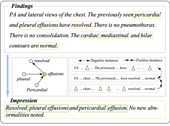
Figure 1: An example of the findings and corresponding impression, where the relation information, as well as positive and negative examples, are also shown in the figure. Note that $\triangle$ represents the removed word.

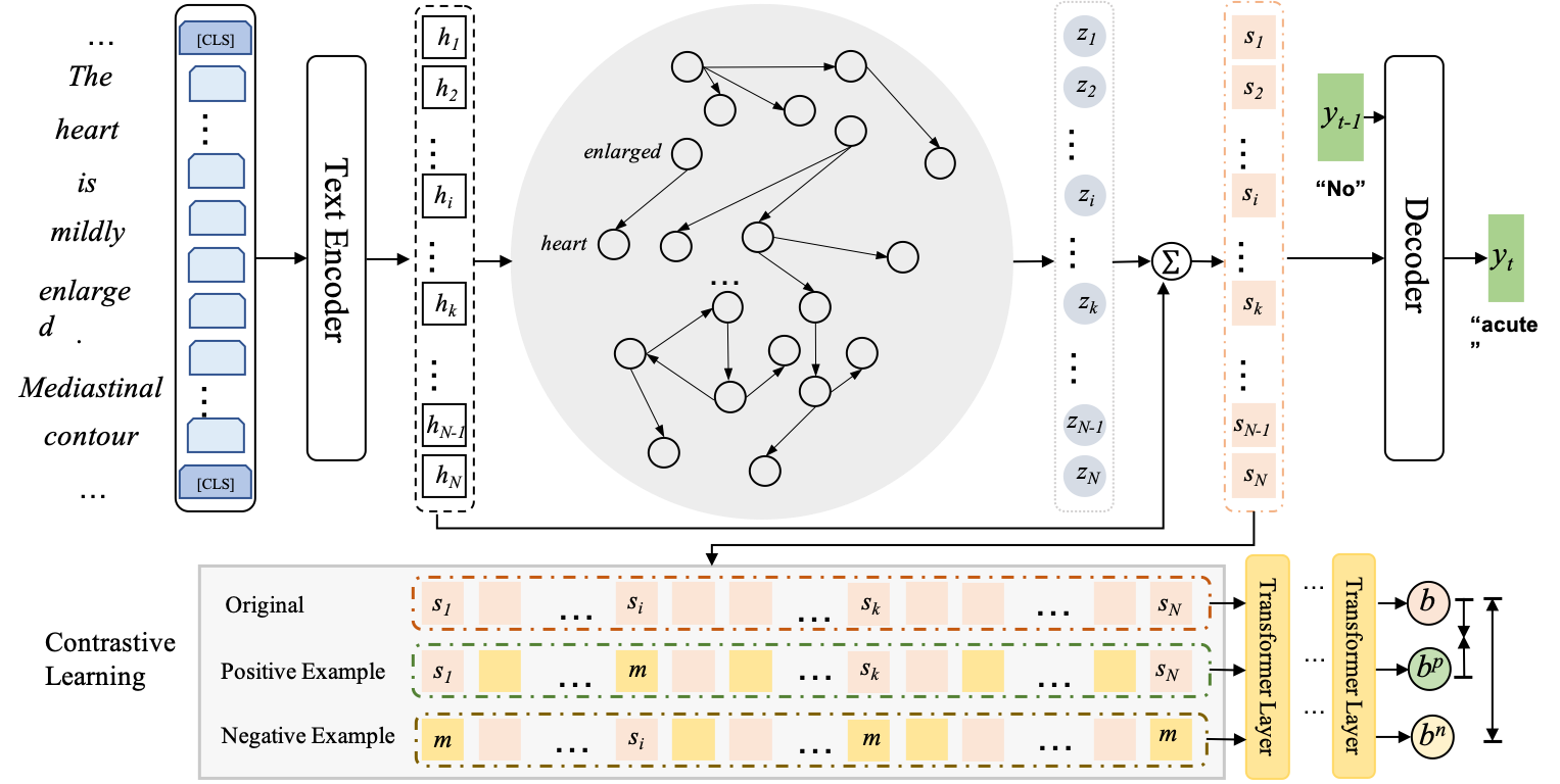
Figure 2: The overall architecture of our proposed method with graph and contrastive learning. An example input and output at $t-1$ and $t$ step are shown in the figure, where the top is the backbone sequence-to-sequence paradigm with a graph to store relation information between critical words and the bottom is the contrastive learning module with specific positive and negative examples. $\mathbf{m}$ refer to a mask vector.

Most existing studies focus on incorporating extra knowledge on the general encoder-decoder framework. For example, Zhang et al. (2018) utilized the background section in the radiology report through a separate encoder and then used it to guide the decoding process to enhance impression generation. Similarly, MacAvaney et al. (2019) and Gharebagh et al. (2020) proposed to extract the ontology information from findings and used an encoder to encode such information to promote the decoding process. Although these approaches have brought significant improvements, they only leverage extra knowledge and findings separately (i.e., through an extra encoder). Thus, their performance relies heavily on the quality of extra knowledge, and the further relationships between extra knowledge and findings are not explored. In this paper, we propose a unified framework to exploit both findings and extra knowledge in an integrated way so that the critical information (i.e., key words and their relations in our paper) can be leveraged in an appropriate way. In detail, for each input findings, we construct a word graph through the automatically extracted entities and dependency tree, with its embeddings, which are from a text encoder. Then, we model the relation information among key words through a graph encoder (e.g., graph neural networks (GNNs)). Finally, contrastive learning is introduced to emphasize key words in findings to map positive samples (constructed by masking non-key words) closer and push apart negative ones (constructed by masking key words), as shown in Figure 1. In such a way, key words and their relations are leveraged in an integrated way through the above two modules (i.e., contrastive learning and the graph encoder) to promote AIG. Experimental results on two datasets (i.e., OpenI and MIMIC-CXR) show that our proposed approach achieves state-of-the-art results.

2 Method

We follow the standard sequence-to-sequence paradigm for AIG. First, we utilize WordPiece Wu et al. (2016) to tokenize original findings and obtain the source input sequence $\mathcal{X}=x_{1},x_{2},\cdots,x_{N}$, where $N$ is the number of tokens in $\mathcal{X}$. The goal is to find a sequence $\mathbf{Y}=\left\{y_{1},...y_{i},...,y_{L}\right\}$ that summarizes the most critical observations in findings, where $L$ is the length of impression and $y_{i}\in\mathrm{V}$ are the generated tokens and $\mathrm{V}$ is the vocabulary of all possible tokens. The generation process can be formalized as:

$$p(\mathbf{Y}\mid\mathcal{X})=\prod_{t=1}^{L}p\left(y_{t}\mid y_{1},\ldots,y_{t-1},\mathcal{X}\right)$$ (1)

The model is then trained to maximize the negative conditional log-likelihood of $\mathcal{Y}$ given the $\mathcal{X}$:

$$\theta^{*}=\underset{\theta}{\arg\max}\sum_{t=1}^{L}\log p\left(y_{t}\mid y_{1},...,y_{t-1},\mathcal{X},A;\theta\right)$$ (2)

where $\theta$ is the parameters of the model, and $A$ represents edges in the relation graph. An overview of our proposed method is presented in Figure 2. Our model contains three main components, i.e., the graph enhanced encoder, the contrastive learning module, and the decoder. The details are described in the following sub-sections.

2.1 Relation Graph

The impression usually describes critical abnormalities with more concise descriptions summarized from the corresponding findings and sometimes uses key phrases to express observations. For example, a sentence in findings texts “There is a left pleural effusion which is small in size.”, is simplified as a key phrase “Small left pleural effusion” in the impression, where the relation between “small” and “effusion” is vital for describing the corresponding observation. Thus, the relation information in findings plays an essential role in accurate key phrase generation. Four types of medical entities, anatomy, observation, anatomy modifier, and observation modifier, are recognized from findings, which compose a majority of important medical knowledge in impression Hassanpour and Langlotz (2016). With WordPiece tokenization, we represent each entity by frequent subwords and connect any two subwords if they are adjacent in the same entity to enhance internal relations for keeping the entity complete. For example, the entity “opacity” is represented as “op ##acity” and then these two subwords connect to each other with both from “op” to “##acity” and from “##acity” to “op”. Besides, we need to consider the semantic relation between entities and other words, such as words used to describe the location and degree of symptoms, which is necessary for accurately recording abnormalities. For example, in a text span “bilateral small pleural effusions”, relations in <“bilateral”,“effusions”>, <“small”,“effusions”> are also important to describe the observation “effusions” and they can be extracted from the dependency tree. Therefore, we construct a dependency tree to extract the semantic relations between entities and other words, with the direction from their head words to themselves. We also employ the WordPiece to split these words as subwords and connect all the source subwords to the corresponding target words with the original direction. The constructed subword graph is then used to extract relation information, with edges represented by $A$.

Algorithm 1: Generation of Examples

Input: $\mathbf{s}$: graph enhanced token representation

$A$: edges in relation graph

Output: $\mathbf{s}^{p}$ Positive example

$\mathbf{s}^{n}$ Negative example

Initialization: $\mathbf{s}^{p}\leftarrow\mathbf{s}$, $\mathbf{s}^{n}\leftarrow\mathbf{s}$

$\mathbf{m}=[1e-6]\in\mathrm{R}^{d}$

1: $N$, $d$ = size($\mathbf{s}$)

2: $V_{key}$ = Extract_subword_index($A$)

3: for $j=0$ to $N$ do

4:   if j in $V_{key}$ then

5:     $\mathbf{s}^{n}_{j}\leftarrow\mathbf{m}$

6:   else:

7:     $\mathbf{s}^{p}_{j}\leftarrow\mathbf{m}$

8:   end if

9: end for

2.2 Graph Enhanced Encoder

In recent years, pre-trained models have dominated not only general summarization tasks but also multi-modal tasks because of their strong ability in feature representation Wu et al. (2021); Zhang et al. (2020a); Yuan et al. (2021, 2022). Thus, in our method, we utilize the pre-trained model BioBERT Lee et al. (2020) trained on a large biomedical corpus as our text encoder. The hidden state $\mathbf{h}_{i}$ for each token $x_{i}$ is generated by the text encoder

$$[\mathbf{h}_{1},\mathbf{h}_{2},\cdots,\mathbf{h}_{n}]={f}_{te}(x_{1},x_{2},\cdots,x_{n})$$ (3)

Herein, ${f}_{te}(\cdot)$ refers to the pre-trained Transformer-based text encoder (i.e., BioBERT Lee et al. (2020)), and $\mathbf{h}_{i}$ is a $d$-dimensional feature vector for representing corresponding tokens $x_{i}$. Since GNNs are well known for extracting features from graph structure and have been shown promising in text generation tasks Jia et al. (2020); Hu et al. (2021), we employ a GNN-based encoder to capture relation information from the corresponding subword graph. This process can be formulated as:

$$\mathbf{z}=f_{ge}(\mathbf{h},A),$$ (4)

where $f_{ge}(\cdot)$ is the graph encoder, and $\mathbf{z}$ is the feature vector extracted from the graph. Next, to incorporate relation information into token representation, we concatenate $\mathbf{z}$ and $\mathbf{h}$ and utilize a fully connected layer to reduce it to the same dimensions as $\mathbf{z}$ and $\mathbf{h}$:

$$\mathbf{s}=\text{MLP}([\mathbf{h}_{1}\oplus\mathbf{z}_{1},\mathbf{h}_{2}\oplus\mathbf{z}_{2},\cdots,\mathbf{h}_{n}\oplus\mathbf{z}_{n}]),$$ (5)

where $\mathbf{s}$ is the final token representation.

2.3 Contrastive Learning

Only relying on a GNN encoder to capture relation information still lacks the capability to fully grasp important word information from findings since the graph is pre-defined before training or testing. Recently, contrastive learning has shown strong power in learning and distinguishing significant knowledge by concentrating positive samples and contrasting with negative samples, and brought significant improvements in many tasks, such as improving the faithfulness of summarization and discriminating vital information to enhance representation Cao and Wang (2021); Zeng et al. (2021). We expect our model to be more sensitive to critical words contained in findings. For this purpose, we apply a contrastive learning module to concentrate positive pairs and push negative ones apart, which aims to help the model differentiate essential information from secondary information. We regard tokens with edges in the relation graph as critical tokens since they contain important information for describing key observations, as discussed in 2.1. To construct a positive example, we mask each non-key token representation in $\mathbf{s}$ as the constant vectors $\mathbf{m}\in\mathbb{R}^{d}$, with all elements $1e-6$, so that this instance can consolidate the critical information and remove unimportant words. Meanwhile, we utilize a similar way to mask important token representations in $\mathbf{s}$ as $\mathbf{m}$ to obtain a negative example $\mathbf{s}^{n}$. The details of generating positive and negative examples are shown in Algorithm 1. Note that in our model, we do not consider the other instances in the same mini-batch as the negative examples, which is different from many existing approaches Kim et al. (2021); Giorgi et al. (2020) since we aim to identify the critical content in $\mathcal{X}$ instead of expanding differences between various findings in one mini-batch. In addition, radiology reports are not as diverse as ordinary texts, and they are mainly composed of fixed medical terms and some attributive words, where the former is used to record critical information and the latter is to keep sentences fluent and grammatically correct.

Afterward, we employ a randomly initialized Transformer-based encoder to model $\mathbf{s}$, $\mathbf{s}^{p}$, $\mathbf{s}^{n}$, respectively, which can be formulated as:

$$\mathbf{b} =f_{ce}(\mathbf{s}),$$ (6)

$$\mathbf{b}^{p} =f_{ce}(\mathbf{s}^{p}),$$ (7)

$$\mathbf{b}^{n} =f_{ce}(\mathbf{s}^{n}),$$ (8)

where $f_{ce}(\cdot)$ represents the contrastive encoder. $\mathbf{b}$, $\mathbf{b}^{p}$ and $\mathbf{b}^{n}$ are intermediate states extracted from the encoder, which are also $d$-dimensional vectors. Then, we calculate cosine similarity $sim(\mathbf{b}^{1},\mathbf{b}^{2})=\frac{\mathbf{b}_{1}^{\top}\mathbf{b}_{2}}{\left\|\mathbf{b}_{1}\right\|\cdot\left\|\mathbf{b}_{2}\right\|}$ for positive and negative pairs, denoted as $sim(\mathbf{b},\mathbf{b}^{p})$ and $sim(\mathbf{b},\mathbf{b}^{n})$. We follow Robinson et al. (2020) to formulate the training objective of contrastive module:

$$l_{con}=-\log\frac{e^{\operatorname{sim}\left(\mathbf{b}_{i},\mathbf{b}^{p}\right)/\tau}}{\sum_{j=1}^{N}\left(e^{\operatorname{sim}\left(\mathbf{b}_{i},\mathbf{b}^{p}\right)/\tau}+e^{\operatorname{sim}\left(\mathbf{b}_{i},\mathbf{b}^{n}\right)/\tau}\right)},$$ (9)

where $\tau$ is a temperature hyperparameter, which is set to 1 in this paper.

2.4 Decoder

The decoder in our model is built upon a standard Transformer Vaswani et al. (2017), where the representation $\mathbf{s}$ is functionalized as the input of the decoder so as to improve the generation process. In detail, $\mathbf{s}$ is sent to the decoder at each decoding step, jointly with the generated tokens from previous steps, and thus the current output $y_{t}$ can be computed by

$$y_{t}=f_{e}(\mathbf{s}_{1},\mathbf{s}_{2},\cdots,\mathbf{s}_{n},y_{1},\cdots,y_{t-1}),$$ (10)

where $f_{e}(\cdot)$ refers to the Transformer-based decoder and this process is repeated until the complete impression is obtained.

Besides, to effectively incorporate the critical word information into the decoding process, we sum the losses from the impression generation and contrastive objectives as

$$L=l_{ge}+\lambda l_{con},$$ (11)

where $l_{ge}$ is the basic sequence-to-sequence loss, and $\lambda$ is the weight to control the contrastive loss.

Data	Type	Train	Dev	Test
OpenI	Report #	2400	292	576
	Avg. wf	37.89	37.77	37.98
	Avg. sf	5.75	5.68	5.77
	Avg. wi	10.43	11.22	10.61
	Avg. si	2.86	2.94	2.82
MIMIC -CXR	Report #	122,014	957	1,606
	Avg. wf	55.78	56.57	70.67
	Avg. sf	6.50	6.51	7.28
	Avg. wi	16.98	17.18	21.71
	Avg. si	3.02	3.04	3.49

Table 1: The statistics of the two benchmark datasets with random split for OpenI and official split for MIMIC-CXR, including the numbers of report, the averaged sentence-based length (Avg. sf, Avg. si), the averaged word-based length (Avg. wf, Avg. wi) of both Impression and Findings.

Data	Model	ROUGE			FC
		R-1	R-2	R-L	P	R	F-1
OpenI	Base	62.74	53.32	62.86	-	-	-
	Base+CL	63.53	54.58	63.13	-	-	-
	Base+graph	63.29	54.12	63.03	-	-	-
	Base+graph+CL	64.97	55.59	64.45	-	-	-
MIMIC-CXR	Base	47.92	32.43	45.83	58.05	50.90	53.01
	Base+CL	48.15	33.25	46.24	58.34	51.58	53.70
	Base+graph	48.29	33.30	46.36	57.80	51.70	53.50
	Base+graph+CL	49.13	33.76	47.12	58.85	52.33	54.52

Table 2: Comparisons of baselines and our method on OpenI and MIMIC-CXR datasets. R-1, R-2 and R-L refer to ROUGE-1, ROUGE-2 and ROUGE-L, respectively. P, R and F-1 represent precision, recall, and F1 score.

3 Experimental Setting

3.1 Dataset

Our experiments are conducted on two following datasets: OpenI Demner-Fushman et al. (2016) and MIMIC-CXR Johnson et al. (2019) respectively, where the former contains 3268 reports collected by Indiana University and the latter is a larger dataset containing 124577 reports. Note that the number of reports we introduced is counted after pre-processing. We follow Hu et al. (2021); Zhang et al. (2018) to filter the reports by deleting the reports in the following cases: (1) no findings or no impression sections; (2) the findings have fewer than ten words, or the impression has fewer than two words. For OpenI, we follow Hu et al. (2021) to randomly divide it into train/validation/test set by 2400:292:576 in our experiments. For MIMIC-CXR, we apply two types of splits, including an official split and a random split with a ratio of 8:1:1 similar to Gharebagh et al. (2020). We report the statistics of these two datasets in Table 1.

Model	OpenI			MIMIC-CXR
	Random split			Official split			Random split
	R-1	R-2	R-L	R-1	R-2	R-L	R-1	R-2	R-L
LexRank Erkan and Radev (2004)	14.63	4.42	14.06	18.11	7.47	16.87	-	-	-
TransExt Liu and Lapata (2019)	15.58	5.28	14.42	31.00	16.55	27.49	-	-	-
PGN (LSTM) See et al. (2017)	63.71	54.23	63.38	46.41	32.33	44.76	-	-	-
TransAbs Liu and Lapata (2019)	59.66	49.41	59.18	47.16	32.31	45.47	-	-	-
$\textsc{OntologyABS}^{\dagger}$ Gharebagh et al. (2020)	-	-	-	-	-	-	53.57	40.78	51.81
$\textsc{WGSum (LSTM)}^{\dagger}$ Hu et al. (2021)	64.32	55.48	63.97	47.48	33.03	45.43	54.97	43.64	53.81
$\textsc{WGSum (Trans)}^{\dagger}$ Hu et al. (2021)	61.63	50.98	61.73	48.37	33.34	46.68	56.38	44.75	55.32
Ours	64.97	55.59	64.45	49.13	33.76	47.12	57.38	45.52	56.13

Table 3: Comparisons of our proposed models with previous study on the OpenI and MIMIC-CXR with respect to ROUGE metric. $\dagger$ refers to that the results is directly cited from the original paper.

3.2 Baseline and Evaluation Metrics

To explore the performance of our method, we use the following ones as our main baselines:

• Base Liu and Lapata (2019): this is a backbone sequence-to-sequence model, i.e., a pre-trained encoder and a randomly initialized Transformer-based decoder.

• Base+graph and Base+CL: these have the same architecture as Base, where the former incorporates an extra graph encoder to enhance relation information, and the latter introduces a contrastive learning module to help the model distinguish critical words.

Besides, we also compare our method with those existing studies, including both extractive summarization methods, e.g., LexRank Erkan and Radev (2004), TransformerEXT Liu and Lapata (2019), and the ones proposed for abstractive models. e.g., TransformerABS Liu and Lapata (2019), OntologyABS Gharebagh et al. (2020), WGSum (Trans+GAT), and WGSum (LSTM+GAT) Hu et al. (2021).

Actually, factual consistency (FC) is critical in radiology report generation Liu et al. (2019); Chen et al. (2020). Following Zhang et al. (2020c); Hu et al. (2021), we evaluate our model and three baselines by two types of metrics: summarization and FC metrics. For summarization metrics, we report $\textsc{F}_{1}$ scores of ROUGE-1 (R-1), ROUGE-2 (R-2), and ROUGE-L (R-L). Besides, for FC metrics, we utilize CheXbert Smit et al. (2020) to detect 14 observations related to diseases from reference impressions and generated impressions and then calculate the precision, recall, and F1 score between these two identified results.

3.3 Implementation Details

In our experiments, we utilize biobert-base-cased-v1.1 as our text encoder and follow its default model settings: we use 12 layers of self-attention with 768-dimensional embeddings. Besides, we employ stanza Zhang et al. (2020d) to extract medical entities and the dependence tree, which is used to construct the graph and generate positive and negative examples. Our method is implemented based on the code of BertSum Liu and Lapata (2019). In addition, we use a 2-layer graph attention networks (GAT) Veličković et al. (2017) with the hidden size of 768 as our graph encoder and a 6-layer Transformer with 768 hidden sizes and 2048 feed-forward filter sizes for the contrastive encoder. The decoder is also a 6-layer Transformer with 768 dimensions, 8 attention heads, and 2048 feed-forward filter sizes. Note that $\lambda$ is set 1 in all experiments, and more detailed hyperparameters are reported in A.1. During the training, we use Adam Kingma and Ba (2014) to optimize the trainable parameters in our model.

4 Results and Analyses

4.1 Effect of Graph and Contrastive learning

To explore the effectiveness of our proposed method, we conduct experiments on two benchmark datasets, with the results reported in Table 2, where Base+graph+CL represents our complete model. We can obtain several observations from the results. First, both Base+graph and Base+CL achieve better results than Base with respect to R-1, R-2, and R-L, which indicates that graph and contrastive learning can respectively promote impression generation. Second, Base+graph+CL outperforms all baselines with significant improvement on two datasets, confirming the effectiveness of our proposed method in combining graph and contrastive learning. This might be because graphs and contrastive learning can provide valuable information from different aspects, the former mainly record relation information, and the latter brings critical words knowledge, so that an elaborate combination of them can bring more improvements. Third, when comparing these two datasets, the performance gains from our full model over three baselines on OpenI are more prominent than that on MIMIC-CXR. This is perhaps because compared to MIMIC-CXR, OpenI dataset is relatively smaller and has a shorter averaged word-based length, such that it is easier for the graph to record relation and more accessible for contrastive learning to recognize key words by comparing positive and negative examples. Fourth, we can find a similar trend on the FC metric on the MIMIC-CXR dataset, where a higher F1 score means that our complete model can generate more accurate impressions thanks to its more substantial power in key words discrimination and relationship information extraction.

4.2 Comparison with Previous Studies

In this subsection, we further compare our models with existing models on the aforementioned datasets, and the results are reported in Table 3. There are several observations. First, the comparison between our model and OntologyABS shows the effectiveness of our design in this task, where our model achieves better performance, though both of them enhance impression generation by incorporating crucial medical information. This might be because by comparing positive and negative examples for each findings, our model is more sensitive to critical information and more intelligent in distinguishing between essential information and secondary information, contributing to more accurate and valuable information embedded in the model. Second, we can observe that our model outperforms all existing models in terms of R-1, R-2, and R-L. On the one hand, effectively combining contrastive learning and graph into the sequence to sequence model is a better solution to improve feature extraction and thus promote the decoding process robustly. On the other hand, the pre-trained model (i.e., BioBERT) used in our model is a more powerful feature extractor in modeling biomedical text than those existing studies, e.g., TransformerABS, OntologyABS, and PGN, which utilize randomly initialized encoders. Third, when compared to those complicated models, e.g., WGSUM utilize stanza to extract entities and construct two extra graph encoders to extract features from a word graph, which are then regarded as background information and dynamic guiding information to enhance the decoding process for improving impression generation, our model can achieve better performance through a somewhat more straightforward method.

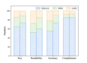
Figure 3: The results of human evaluation, where forward and backslash represent that Base+graph+CL versus the reference and Base, respectively. Yellow, green and blue represent that our model loses, equal to competitors and wins.

4.3 Human Evaluation

We further conduct a human evaluation to understand the quality of the generated impression better and alleviate the limitation of the ROUGE metric. One hundred generated impressions on MIMIC-CXR from Base and Base+graph+CL, along with their corresponding reference impressions, are randomly selected for expert evaluation Gharebagh et al. (2020). Besides, we follow Hu et al. (2021) to utilize four metrics: Key, Readability, Accuracy, and Completeness, respectively. We invite three medical experts to score these generated impressions based on these four metrics, with the results shown in Figure 3. On the one hand, compared to Base, we can find that our model outperforms it on all four metrics, where 16%, 25%, 18%, and 8% of impressions from our model obtain higher quality than Base. On the other hand, comparing our model against reference impressions, our model obtains close results on key, accuracy, and completeness, with 86%, 78%, and 92% of our model outputs being at least as good as radiologists, while our model is less preferred for readability with a 10% gap. The main reason might be that many words removed in positive examples are used to keep sequence fluently, and our model tends to identify them as secondary information, leading that our model obtains relatively worse results on the readability metric.

4.4 Analyses

We conduct further analyses on Findings Length and Case Study.

Findings Length

To test the effectiveness of the word-based length of findings, we categorize the findings on the MIMIC-CXR test set into seven groups and present the R-1 score for each group in Figure 4. We have the following observations. First, as the findings length becomes long, the performance of Base and our model tend to decrease, except for the second group, i.e., [25, 45], since short text are more accessible for the encoder to capture valid features, which is consistent with previous studies Dai et al. (2019). Second, our model outperforms Base in all the groups, further illustrating the effectiveness of our model regardless of the findings length. Third, we can observe a grey line with a downward trend from the incremental chart in the upper right corner of Figure 4, indicating that our model (i.e., Base+graph+CL) tends to gain better improvements over Base on shorter findings than that on longer ones. This is because longer findings usually contain relatively more secondary information such that it is more challenging for contrastive learning to distinguish critical knowledge.

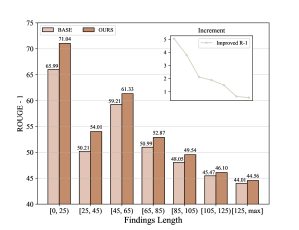
Figure 4: R-1 score of generated impressions from Base and our model on the MIMIC-CXR test set, where OURS represent the Base+graph+CL.

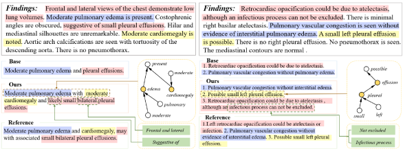
Figure 5: Examples of the generated impressions from Base and Base+graph+CL as well as reference impressions. The yellow nodes in the graph indicate that these words are contained in entities.

Case study

To further demonstrate how our approach with graph and contrastive learning helps the generation of findings, we perform qualitative analysis on two cases, and the results are shown in Figure 5, where different colors on the texts indicate different critical information. Compared to Base model, our model can generate more complete impressions which cover almost all the crucial abnormalities. In contrast, the Base model fails to identify all the key information, e.g., (“moderate cardiomegaly” in the left example and “possible small left pleural effusion” in the right case). Besides, our model can generate more accurate impressions with an appropriate word to represent possibility and a better modifier to describe the observation. On the one hand, in Figure 5, “suggestive of” in the left example and “may” in the right example imply a type of uncertainty, which means that doctors wonder whether the abnormal observation exists when writing findings, so that the corresponding word (i.e., “likely”) is used to describe this sensitive information. On the other hand, in the left case, according to the phrase “Frontal and lateral” in its original findings, our model can generate the synonym “bilateral” to depict the symptom “pleural effusions” more specifically.

5 Related Work

Recently, NLP technology has broadly applied in the medical domain, such as medical entity recognition Liu et al. (2021b); Zhao et al. (2019), radiology report generation Chen et al. (2021); Zhang et al. (2020b); Liu et al. (2021a), AIG, etc. Impression generation can be regarded as a type of summarization task that has drawn substantial attention in recent years, and there are many studies for addressing general abstractive summarization See et al. (2017); Li et al. (2020); You et al. (2019); Huang et al. (2020). You et al. (2019) designed a novel focus-attention mechanism and saliency-selection network, equipped in the encoder and decoder to enhance summary generation. Li et al. (2020) proposed an abstractive sentence summarization method guided by the key words, which utilized a dual-attention and a dual-copy mechanism to integrate the semantics of both original sequence and key words. Many methods propose to introduce specific designs on the general summarization model to address radiology impression generation Zhang et al. (2018); Gharebagh et al. (2020); MacAvaney et al. (2019); Hu et al. (2021); Abacha et al. (2021). MacAvaney et al. (2019); Gharebagh et al. (2020) extracted the salient clinical ontology terms from findings and then incorporated them into the summarizer through a separate encoder for enhancing AIG. Hu et al. (2021) further introduced pre-defined word graphs to record salient words as well as their internal relation and then employed two separate graph encoders to leverage graphs for guiding the decoding process. Most of these approaches exploit separate encoders to encode pre-defined knowledge (e.g., ontology terms and word graph), which are then utilized to enhance impression generation. However, they tend to over-rely on the quality of pre-extracted ontologies and word graphs and lack sensitivity to vital information of findings themselves. Compared to these models, our method offers an alternative solution to robustly improve key information extraction with the help of both graphs and contrastive learning.

6 Conclusion

In this paper, we propose to combine graphs and contrastive learning to better incorporate valuable features for promoting impression generation. Specifically, we utilize the graph encoder to extract relation information from the graph, constructed by medical entities and the dependence tree, for enhancing the representation from the pre-trained text encoder. In addition, we employ contrastive learning to assist the model in distinguishing between critical and secondary information, simultaneously improving sensitivity to important word representation by comparing positive and negative examples. Furthermore, we conduct experiments on two benchmark datasets, and the results illustrate the effectiveness of our proposed method, where new state-of-the-art results are achieved.

Appendix A Appendix

A.1 Hyper-parameter Settings

Table 4 reports the hyper-parameters tested in tuning our models on MIMIC-CXR and OpenI. For each dataset, we try all combinations of the hyper-parameters and use the one achieving the highest R-1 for MIMIC-CXR and OpenI.

Model	Hyper-Parameter	Value
MIMIC-CXR	Batch Size	32,64,128,300
	Learning Rate	8e-5,2e-4, 1e-3, 0.05,
	Training steps	150000
OpenI	Batch Size	32,64,128,300
	Learning Rate	8e-5,5e-3, 1e-3, 0.05
	Training steps	20000

Table 4: The hyper-parameters that we have experimented on the datasets. The bold values illustrates the best configurations of different models.

References

- Abacha et al. (2021) Asma Ben Abacha, Yassine M’rabet, Yuhao Zhang, Chaitanya Shivade, Curtis Langlotz, and Dina Demner-Fushman. 2021. Overview of the Mediqa 2021 Shared Task on Summarization in the Medical Domain. In Proceedings of the 20th Workshop on Biomedical Language Processing, pages 74–85.
- Cao and Wang (2021) Shuyang Cao and Lu Wang. 2021. CLIFF: Contrastive Learning for Improving Faithfulness and Factuality in Abstractive Summarization. arXiv preprint arXiv:2109.09209.
- Chen et al. (2021) Zhihong Chen, Yaling Shen, Yan Song, and Xiang Wan. 2021. Cross-modal Memory Networks for Radiology Report Generation. In Proceedings of the 59th Annual Meeting of the Association for Computational Linguistics and the 11th International Joint Conference on Natural Language Processing (Volume 1: Long Papers), pages 5904–5914.
- Chen et al. (2020) Zhihong Chen, Yan Song, Tsung-Hui Chang, and Xiang Wan. 2020. Generating Radiology Reports via Memory-driven Transformer. In Proceedings of the 2020 Conference on Empirical Methods in Natural Language Processing (EMNLP), pages 1439–1449.
- Dai et al. (2019) Zihang Dai, Zhilin Yang, Yiming Yang, Jaime G Carbonell, Quoc Le, and Ruslan Salakhutdinov. 2019. Transformer-XL: Attentive Language Models beyond a Fixed-Length Context. In Proceedings of the 57th Annual Meeting of the Association for Computational Linguistics, pages 2978–2988.
- Demner-Fushman et al. (2016) Dina Demner-Fushman, Marc D Kohli, Marc B Rosenman, Sonya E Shooshan, Laritza Rodriguez, Sameer Antani, George R Thoma, and Clement J McDonald. 2016. Preparing a Collection of Radiology Examinations for Distribution and Retrieval. Journal of the American Medical Informatics Association, 23(2):304–310.
- Erkan and Radev (2004) Günes Erkan and Dragomir R Radev. 2004. Lexrank: Graph-based Lexical Centrality as Salience in Text Summarization. Journal of artificial intelligence research, 22:457–479.
- Gharebagh et al. (2020) Sajad Sotudeh Gharebagh, Nazli Goharian, and Ross Filice. 2020. Attend to Medical Ontologies: Content Selection for Clinical Abstractive Summarization. In Proceedings of the 58th Annual Meeting of the Association for Computational Linguistics, pages 1899–1905.
- Giorgi et al. (2020) John M Giorgi, Osvald Nitski, Gary D Bader, and Bo Wang. 2020. Declutr: Deep Contrastive Learning for Unsupervised Textual Representations. arXiv preprint arXiv:2006.03659.
- Hassanpour and Langlotz (2016) Saeed Hassanpour and Curtis P Langlotz. 2016. Information Extraction from Multi-institutional Radiology Reports. Artificial intelligence in medicine, 66:29–39.
- Hu et al. (2021) Jinpeng Hu, Jianling Li, Zhihong Chen, Yaling Shen, Yan Song, Xiang Wan, and Tsung-Hui Chang. 2021. Word Graph Guided Summarization for Radiology Findings. In Findings of the Association for Computational Linguistics: ACL-IJCNLP 2021, pages 4980–4990.
- Huang et al. (2020) Luyang Huang, Lingfei Wu, and Lu Wang. 2020. Knowledge Graph-Augmented Abstractive Summarization with Semantic-Driven Cloze Reward. In Proceedings of the 58th Annual Meeting of the Association for Computational Linguistics, pages 5094–5107.
- Jia et al. (2020) Ruipeng Jia, Yanan Cao, Hengzhu Tang, Fang Fang, Cong Cao, and Shi Wang. 2020. Neural Extractive Summarization with Hierarchical Attentive Heterogeneous Graph Network. In Proceedings of the 2020 Conference on Empirical Methods in Natural Language Processing (EMNLP), pages 3622–3631.
- Johnson et al. (2019) Alistair EW Johnson, Tom J Pollard, Nathaniel R Greenbaum, Matthew P Lungren, Chih-ying Deng, Yifan Peng, Zhiyong Lu, Roger G Mark, Seth J Berkowitz, and Steven Horng. 2019. MIMIC-CXR-JPG, a Large Publicly Available Database of Labeled Chest Radiographs. arXiv preprint arXiv:1901.07042.
- Kim et al. (2021) Taeuk Kim, Kang Min Yoo, and Sang-goo Lee. 2021. Self-guided Contrastive Learning for BERT Sentence Representations. arXiv preprint arXiv:2106.07345.
- Kingma and Ba (2014) Diederik P Kingma and Jimmy Ba. 2014. Adam: A method for stochastic optimization. arXiv preprint arXiv:1412.6980.
- Lee et al. (2020) Jinhyuk Lee, Wonjin Yoon, Sungdong Kim, Donghyeon Kim, Sunkyu Kim, Chan Ho So, and Jaewoo Kang. 2020. Biobert: a Pre-trained Biomedical Language Representation Model for Biomedical Text Mining. Bioinformatics, 36(4):1234–1240.
- Li et al. (2020) Haoran Li, Junnan Zhu, Jiajun Zhang, Chengqing Zong, and Xiaodong He. 2020. Keywords-Guided Abstractive Sentence Summarization. In Proceedings of the AAAI Conference on Artificial Intelligence, volume 34, pages 8196–8203.
- Liu et al. (2021a) Guangyi Liu, Yinghong Liao, Fuyu Wang, Bin Zhang, Lu Zhang, Xiaodan Liang, Xiang Wan, Shaolin Li, Zhen Li, Shuixing Zhang, et al. 2021a. Medical-vlbert: Medical visual language bert for covid-19 ct report generation with alternate learning. IEEE Transactions on Neural Networks and Learning Systems, 32(9):3786–3797.
- Liu et al. (2019) Guanxiong Liu, Tzu-Ming Harry Hsu, Matthew McDermott, Willie Boag, Wei-Hung Weng, Peter Szolovits, and Marzyeh Ghassemi. 2019. Clinically Accurate Chest X-Ray Report Generation. In Machine Learning for Healthcare Conference, pages 249–269. PMLR.
- Liu and Lapata (2019) Yang Liu and Mirella Lapata. 2019. Text Summarization with Pretrained Encoders. In Proceedings of the 2019 Conference on Empirical Methods in Natural Language Processing and the 9th International Joint Conference on Natural Language Processing (EMNLP-IJCNLP), pages 3721–3731.
- Liu et al. (2021b) Yang Liu, Yuanhe Tian, Tsung-Hui Chang, Song Wu, Xiang Wan, and Yan Song. 2021b. Exploring Word Segmentation and Medical Concept Recognition for Chinese Medical Texts. In Proceedings of the 20th Workshop on Biomedical Language Processing, pages 213–220.
- MacAvaney et al. (2019) Sean MacAvaney, Sajad Sotudeh, Arman Cohan, Nazli Goharian, Ish Talati, and Ross W Filice. 2019. Ontology-aware Clinical Abstractive Summarization. In Proceedings of the 42nd International ACM SIGIR Conference on Research and Development in Information Retrieval, pages 1013–1016.
- Robinson et al. (2020) Joshua Robinson, Ching-Yao Chuang, Suvrit Sra, and Stefanie Jegelka. 2020. Contrastive Learning with Hard Negative Samples. arXiv preprint arXiv:2010.04592.
- See et al. (2017) Abigail See, Peter J Liu, and Christopher D Manning. 2017. Get To the Point: Summarization with Pointer-Generator Networks. In Proceedings of the 55th Annual Meeting of the Association for Computational Linguistics (Volume 1: Long Papers), pages 1073–1083.
- Shieh et al. (2019) Alexander Te-Wei Shieh, Yung-Sung Chuang, Shang-Yu Su, and Yun-Nung Chen. 2019. Towards Understanding of Medical Randomized Controlled Trials by Conclusion Generation. In Proceedings of the Tenth International Workshop on Health Text Mining and Information Analysis (LOUHI 2019), pages 108–117.
- Smit et al. (2020) Akshay Smit, Saahil Jain, Pranav Rajpurkar, Anuj Pareek, Andrew Y Ng, and Matthew Lungren. 2020. Chexbert: Combining Automatic Labelers and Expert Annotations for Accurate Radiology Report Labeling Using BERT. In Proceedings of the 2020 Conference on Empirical Methods in Natural Language Processing (EMNLP), pages 1500–1519.
- Vaswani et al. (2017) Ashish Vaswani, Noam Shazeer, Niki Parmar, Jakob Uszkoreit, Llion Jones, Aidan N Gomez, Łukasz Kaiser, and Illia Polosukhin. 2017. Attention is All You Need. In Proceedings of the 31st International Conference on Neural Information Processing Systems, pages 6000–6010.
- Veličković et al. (2017) Petar Veličković, Guillem Cucurull, Arantxa Casanova, Adriana Romero, Pietro Lio, and Yoshua Bengio. 2017. Graph Attention Networks. arXiv preprint arXiv:1710.10903.
- Wu et al. (2021) Wenhao Wu, Wei Li, Xinyan Xiao, Jiachen Liu, Ziqiang Cao, Sujian Li, Hua Wu, and Haifeng Wang. 2021. BASS: Boosting Abstractive Summarization with Unified Semantic Graph. In Proceedings of the 59th Annual Meeting of the Association for Computational Linguistics and the 11th International Joint Conference on Natural Language Processing (Volume 1: Long Papers), Online. Association for Computational Linguistics.
- Wu et al. (2016) Yonghui Wu, Mike Schuster, Zhifeng Chen, Quoc V Le, Mohammad Norouzi, Wolfgang Macherey, Maxim Krikun, Yuan Cao, Qin Gao, Klaus Macherey, et al. 2016. Google’s Neural Machine Translation System: Bridging the gap between Human and Machine Translation. arXiv preprint arXiv:1609.08144.
- You et al. (2019) Yongjian You, Weijia Jia, Tianyi Liu, and Wenmian Yang. 2019. Improving Abstractive Document Summarization with Salient Information Modeling. In Proceedings of the 57th Annual Meeting of the Association for Computational Linguistics, pages 2132–2141.
- Yuan et al. (2022) Zhihao Yuan, Xu Yan, Yinghong Liao, Yao Guo, Guanbin Li, Zhen Li, and Shuguang Cui. 2022. X-trans2cap: Cross-modal knowledge transfer using transformer for 3d dense captioning. arXiv preprint arXiv:2203.00843.
- Yuan et al. (2021) Zhihao Yuan, Xu Yan, Yinghong Liao, Ruimao Zhang, Zhen Li, and Shuguang Cui. 2021. Instancerefer: Cooperative holistic understanding for visual grounding on point clouds through instance multi-level contextual referring. In Proceedings of the IEEE/CVF International Conference on Computer Vision, pages 1791–1800.
- Zeng et al. (2021) Zhiyuan Zeng, Keqing He, Yuanmeng Yan, Zijun Liu, Yanan Wu, Hong Xu, Huixing Jiang, and Weiran Xu. 2021. Modeling Discriminative Representations for Out-of-Domain Detection with Supervised Contrastive Learning. arXiv preprint arXiv:2105.14289.
- Zhang et al. (2020a) Jingqing Zhang, Yao Zhao, Mohammad Saleh, and Peter Liu. 2020a. Pegasus: Pre-training with Extracted Gap-Sentences for Abstractive Summarization. In International Conference on Machine Learning, pages 11328–11339. PMLR.
- Zhang et al. (2020b) Yixiao Zhang, Xiaosong Wang, Ziyue Xu, Qihang Yu, Alan Yuille, and Daguang Xu. 2020b. When Radiology Report Generation Meets Knowledge Graph. In Proceedings of the AAAI Conference on Artificial Intelligence, volume 34, pages 12910–12917.
- Zhang et al. (2018) Yuhao Zhang, Daisy Yi Ding, Tianpei Qian, Christopher D Manning, and Curtis P Langlotz. 2018. Learning to Summarize Radiology Findings. In Proceedings of the Ninth International Workshop on Health Text Mining and Information Analysis, pages 204–213.
- Zhang et al. (2020c) Yuhao Zhang, Derek Merck, Emily Tsai, Christopher D Manning, and Curtis Langlotz. 2020c. Optimizing the Factual Correctness of a Summary: A Study of Summarizing Radiology Reports. In Proceedings of the 58th Annual Meeting of the Association for Computational Linguistics, pages 5108–5120.
- Zhang et al. (2020d) Yuhao Zhang, Yuhui Zhang, Peng Qi, Christopher D Manning, and Curtis P Langlotz. 2020d. Biomedical and Clinical English Model Packages in the Stanza Python NLP Library. arXiv preprint arXiv:2007.14640.
- Zhao et al. (2019) Sendong Zhao, Ting Liu, Sicheng Zhao, and Fei Wang. 2019. A Neural Multi-Task Learning Framework to Jointly Model Medical Named Entity Recognition and Normalization. In Proceedings of the AAAI Conference on Artificial Intelligence, volume 33, pages 817–824.