Adaptive Mean-Residue Loss for Robust Facial Age Estimation

Abstract

Automated facial age estimation has diverse real-world applications in multimedia analysis, e.g., video surveillance, and human-computer interaction. However, due to the randomness and ambiguity of the aging process, age assessment is challenging. Most research work over the topic regards the task as one of age regression, classification, and ranking problems, and cannot well leverage age distribution in representing labels with age ambiguity. In this work, we propose a simple yet effective loss function for robust facial age estimation via distribution learning, i.e., adaptive mean-residue loss, in which, the mean loss penalizes the difference between the estimated age distribution’s mean and the ground-truth age, whereas the residue loss penalizes the entropy of age probability out of dynamic top-K in the distribution. Experimental results in the datasets FG-NET and CLAP2016 have validated the effectiveness of the proposed loss. Our code is available at https://github.com/jacobzhaoziyuan/AMR-Loss.

Index Terms—  Age estimation, label distribution learning, deep learning, neural networks.

1 Introduction

Automated facial age estimation has been widely applied to different multimedia application scenarios but remains a very challenging task. Human face aging is a complicated and random process affected by various internal factors, e.g., genes, makeup, living environment. As a result, there are noticeable variances in facial appearance among different subjects with similar ages. Furthermore, the aging process of each subject is lasting, making it hard to perceive the variances in its facial appearance among neighbouring ages.

The research work for facial age estimation in the literature can be classified into three categories, i.e., regression-based [1, 2], classification-based [3], and ranking-based [4, 5]. But these methods fail to address the age distribution effectively, as there are no clear boundaries between adjacent ages, it is relatively easy for humans to guess the age with some confidence. For example, one person could guess a girl is around $25$ years old, or she may be in her mid-$20$s. In real life, the guessing process follows some certain probability distribution, which means that we could convert the mission of age estimation into a process of age distribution learning. In [6], the authors assumed that the age distribution follows a Gaussian distribution with a particular mean age, $m_{i}$, and a standard deviation, $\sigma_{i}$, for $i$-th image, and proposed a novel mean-variance loss. The mean-variance loss attempts to penalize the variance between $m_{i}$ and the ground-truth age, $y_{i}$, by mean loss, and concentrate more on the classes around $m_{i}$ by variance loss. However, it is possible that the two loss functions suppress each other in part of the age distribution, achieving undesired solutions, and even worse, if $y_{i}$ happens to be out of the range $[m_{i}-\sigma_{i},~{}m_{i}+\sigma_{i}]$, variance loss penalizes the softmax loss that attempts to increase the probability of $y_{i}$. Furthermore, the age distributions of different subjects vary a lot, and it is not true that smaller $\sigma_{i}$ leads to a more accurate $m_{i}$.

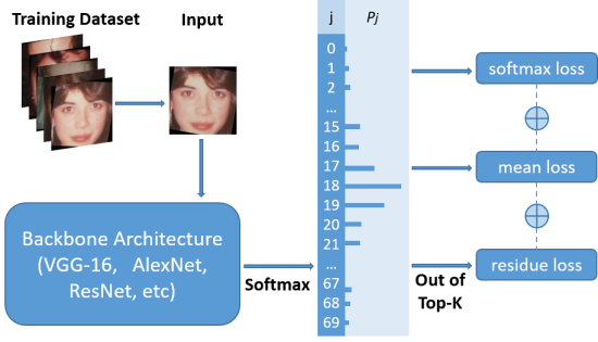
Fig. 1: Overview of the proposed approach

On the other hand, the top-K accuracy of deep learning models has achieved a very high level, e.g., the best top-5 accuracy on the ImageNet dataset is $98\%$ [7]. In age estimation, we can assume that $y_{i}$ is included in top-K classes and the ages out of top-K have a very limited correlation with $y_{i}$, and then the sum of out-of-top-K probabilities can be treated as residue [8]. However, how to determine K remains a problem. These motivate us to propose a hypothesis: If it is hard to extract deeper facial features, why not suppress uncorrelated features and dynamically penalize the residue to strengthen the correlation among the top-K classes indirectly?

In this work, we design an adaptive entropy-based residue loss, which can penalize the age probabilities out of dynamic top-K. By combining mean loss with residue loss, we proposed a simple, yet very efficient loss, adaptive mean-residue loss, for facial age estimation. The proposed mean-residue loss is simple to incorporate into other networks, such as ResNet. Experimental results are superior to the existing state-of-the-art benchmarks, e.g., mean-variance loss.

2 Related Work

Early age estimation work was carried out in [9], where ages were simply split into the following categories, i.e., babies, young and senior individuals. Since then, more and more research interests have been attracted to age estimation from facial images [5, 1]. Traditional methods for facial age estimation consist of two separate stages: feature extraction and one of age regression, classification, and ranking-based methods. In [10], an active appearance model (AAM) was proposed to use shape landmarks and textural features for age estimation. In [11], age estimation is achieved by multi-direction and multi-scale Gabor filters with the feature pooling function were used for identification of biologically inspired features (BIF), but it still relied on feature representations crafted by hand, which is suboptimal to facial age estimation.

Deep learning based approaches have succeeded in many tasks, e.g., object detection [12, 13], image classification [14, 15], biomedical signal processing [16, 17, 18], and medical image analysis [19, 20, 21]. They also have remarkably advanced facial age estimation recently. In [22], deep convolutional neural networks (DCNNs) were proposed to extract features from different regions on facial images and a square loss was utilized for age prediction. In [23], a multi-task deep learning model was proposed for joint estimation based on numerous attributes, including shared feature extraction and attribute group feature extraction. To encode both the ordinal information between adjacent ages and their correlation, soft-ranking label encoding was proposed in [24], which encourages deep learning models to learn more robust facial features for age estimation.

On the other hand, label distribution learning (LDL) was proposed to distinguish label ambiguity, which is challenging. [25, 8]. In LDL, a label distribution can be assigned to an sample. Moreover, the correlation among values in the label space can be leveraged, from which a more robust estimation can be obtained. Gang et al. proposed several LDL based methods for age estimation and presented the robustness of them, e.g., maximum-entropy modeling [26]. It has been argued that a single facial image facilitates not only the estimation of a singular age, but is also informative for adjacent ages [27]. In [6], novel loss functions for model training were proposed and the mean-variance loss was proposed, in which the mean loss aims at minimizing the distance between the predicted age and ground-truth, while the variance loss attempts to lower the variance in the predicted age distribution. Consequently, the age distribution could be sharpened. Meanwhile, a sharper age distribution does not necessarily lead to better age estimation. Under particular circumstances, mean loss and variance loss contradict each other and prevent the accurate prediction to be achieved. In [8], residue loss was proposed to penalize residue errors of the long tails in the distribution for traffic prediction. We advanced the mean-residue loss in an adaptive manner for robust facial age estimation. More details of loss analysis are discussed in Section 4.

3 Preliminary

In an age estimation dataset, $y_{i}\in\{1,2,\ldots,L\}$ represents the corresponding age of $i$-th sample, $x_{i}$ stands for the facial feature, and $f(x_{i})\in\mathbb{R}^{N\times M}$ represents the output from the layer, followed by a last fully connected (FC) layer. Let $z\in\mathbb{R}^{N\times L}$ be the output vector from the last FC layer, and $p\in\mathbb{R}^{N\times L}$ is the softmax probability defined in Equ.1:

$$z=f(x_{i})\cdot\theta^{T};~{}~{}~{}p_{i,j}=\frac{e^{z_{i,j}}}{\sum_{l=1}^{L}e^{z_{i,l}}},$$ (1)

in which $x_{i}$ denotes the feature vector, $\theta\in\mathbb{R}^{L\times M}$ contains trainable parameters in the FC layer, $z_{i,j}$ is an element of $z$ in the $i$-th sample with age $j$. $p_{i,j}$ represents the probability that the age of sample $i$ is $j$. Hence, the estimated or mean age $m_{i}$ of the sample $i$ is calculated in Equ. 2:

$$E(age_{i})=m_{i}=\sum_{j=1}^{L}j\cdot p_{i,j}.$$ (2)

4 Methodology

As illustrated in Fig. 1, the proposed adaptive mean-residue loss can be embedded into a deep convolutional neural network (DCNN) for end-to-end learning. As illustrated in Fig. 2, the proposed adaptive mean-residue loss penalizes (a) the difference between the mean of the estimated age distribution and the ground-truth age, and (b) residue errors in the two long tails of the age distribution.

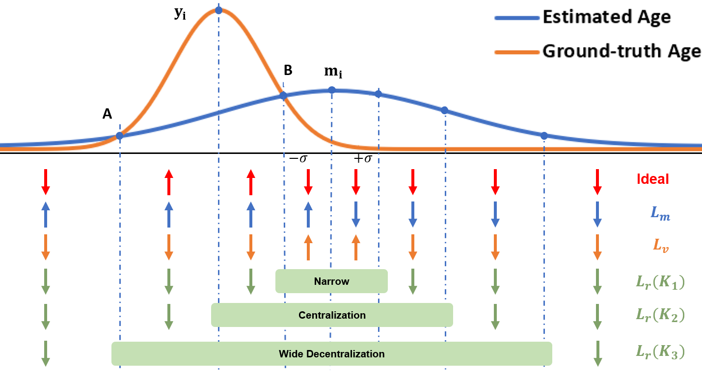
Fig. 2: Gradient analysis on different components of the loss functions. ($L_{m}$: the mean loss, $L_{v}$: the variance loss, $L_{r}$: the residue loss, where $K_{1},K_{2}$ and $K_{3}$ denote three different situations.) $\uparrow$ and $\downarrow$ indicate the direction in which the loss function optimizes the distribution, while the ideal direction is indicated (red). For simplicity, $-\sigma$, $B$, and $K_{1}$ overlap; $y_{i}$ and $K_{2}$ overlap; $A$ and $K_{3}$ overlap.

4.1 Mean Loss

The mean loss suppresses the variance between an estimated age distribution’s mean and the true age. According to Equ. 2, we define the mean loss as

$$L_{m}=\frac{1}{2N}\sum_{i=1}^{N}(m_{i}-y_{i})^{2}=\frac{1}{2N}\sum_{i=1}^{N}(\sum_{j=1}^{L}j\cdot p_{i,j}-y_{i})^{2},$$ (3)

in which $N$, $m_{i}$, and $y_{i}$ are the training batch size, the estimated age, and and ground-truth age, respectively. Unlike the widely used softmax loss, the mean loss is presented in many regression problems. $L_{2}$ distance can be used to evaluate the variances between the mean of an estimated age distribution and the ground-truth age. Therefore, the proposed mean loss complements the softmax loss during training.

4.2 Residue Loss

The residue loss penalizes the residue errors in the tails that exist in an estimated age distribution after the top-K pooling operation. The residue entropy is presented as follows,

$$L_{r}=-\frac{1}{N}\sum_{i=1}^{N}~{}\sum_{j=1,j~{}\notin top-K}^{L}p_{i,j}\cdot\log p_{i,j}.$$ (4)

The mean-variance loss [6] tries to suppress the probabilities within the range $m_{i}\in(j\in[1,m_{i}-\sigma])\cup[m_{i}+\sigma,L])$, where $\sigma$ is the standard deviation of the age distribution in the $i$-th sample. However, inevitably, $y_{i}$ may probably fall inside this range. In this regard, $p_{i,y_{i}}$ is incorrectly suppressed, which could induce errors, while our residue loss $L_{r}$ guarantees that $y_{i}$ falls in the top-K classes and avoids such errors that occur with the mean-variance loss. To further optimize the residue loss, we propose a dynamic top-K pooling method. More specifically, let $K_{i}$ denote the number of top-K. Let $R_{y_{i}}$ stands for the ranking of $y_{i}$, for $i$-th image in a training batch. Subsequently, we can set $K_{i}$ to be adaptive as:

$$K_{i}=max\{2,R_{y_{i}}\}.$$ (5)

With the dynamic top-K pooling, $y_{i}$ is always included during the optimization process, and will not be incorrectly penalized by the residue loss.

4.3 Adaptive Mean-Residue Loss

Combining with the softmax loss $L_{s}$, the adaptive mean-residue loss is showed in Equ. 6:

$$L =L_{s}+\lambda_{1}L_{m}+\lambda_{2}L_{r}$$ (6)

$$=\frac{1}{N}\sum_{i=1}^{N}[-\log p_{i,y_{i}}+\frac{\lambda_{1}}{2}(m_{i}-y_{i})^{2}+\lambda_{2}r_{i}],$$

where $\lambda_{1}$ and $\lambda_{2}$ are hyperparameters that attempt to balance the influences of mean and residue sub-losses in the combined loss function. We use SGD [14] to optimize parameters in the network. At inference, the estimated age of the $i$-th test image can be calculated based on Equ. 2.

4.4 Gradient Analysis

4.4.1 Comparison with Mean-Variance Loss

The mean-variance loss and the mean-residue loss share the same mean loss function. The key difference exists in the variance loss and the residue loss, and their joint effect with the mean loss, as plotted in Fig. 2. In the mean-variance loss, the variance loss attempts to enhance the probabilities of classes within the range of $[m_{i}-\sigma,m_{i}+\sigma]$ while suppressing the probabilities of classes out of the range, no matter $y_{i}$ is in the range or not. When $y_{i}$ is out of the range, variance loss will decrease the probability of $y_{i}$, leading to a worse effect on the model performance. In the mean-residue loss, the residue loss attempts to suppress the probabilities of the classes out of top-K and help the network to focus more on the top-K classes indirectly. Adaptive top-K guarantees that $y_{i}$ is within top-K and residue loss function can help the network to increase the probability of classes within top-K as a whole. Hence, the performance of softmax loss can be enhanced.

4.4.2 Situations of Different K

The joint effect of the mean and residue loss is dependent on the choice of top-K in the residue loss. A proper selection of $K$ is the key to ensuring the correct optimization. The analysis of top-K is illustrated in Fig. 2, and different situations of top-K are summarized as follows: (1) Over Centralization: When top-K is too narrow, e.g., $K_{1}$ in Fig. 2, the ground-truth $y_{i}$ is excluded from the over-centralized top-K classes. The probability at $y_{i}$ is penalized by the residue loss in the wrong direction, and the residue loss conflicts with the mean loss at $y_{i}$, which is undesired. (2) Centralization: When top-K is appropriate, e.g., $K_{2}$ in Fig. 2, the ground-truth $y_{i}$ is included in the centralized top-K classes. The residue loss at $y_{i}$ is 0, and the joint effect of both mean and residue loss are the same as the ideal direction, which is desired. (3) Decentralization: When top-K is too wide, e.g., $K_{3}$ in Fig. 2, the ground-truth $y_{i}$ is included in the decentralized top-K classes. The joint effect of the loss functions is therefore following the ideal optimization direction. However, too many classes are covered by the top-K, in which the residue loss is not calculated. It lessens the effect of the residue loss and makes it more difficult to optimize the model.

Compared with a fixed $K$, the proposed dynamic top-K pooling can obtain a proper range for centralizing the age distribution. As the training proceeds, the distributions of the prediction converge towards the ground-truth, during which the optimal $K$ also decreases. Empirically, a fixed $K$ is either too small at the start of training, excluding $y_{i}$ from top-K pooling, or too large towards the end of the training, slowing down the optimization process. In contrast, the adaptive $K$, as shown in Equ. 5, always includes $y_{i}$ without over centralization or decentralization. Therefore it does not suffer from the drawbacks of a fixed $K$. From our theoretical analysis, we can anticipate that the adaptive mean-residue loss shall outperform the mean-variance loss in accuracy and convergence.

5 Experiments

5.1 Datasets and Evaluation Metrics

Extensive experiments have been carried out using the proposed loss on two popular facial image datasets, i.e., FG-NET [28] and CLAP 2016 [29]. The ages of subjects lie between 0 to 69 years old. We adopt the leave-one-person-out (LOPO) protocol in the experiments [6]. CLAP2016 [29] is a competition dataset released in $2016$ at the ChaLearn Looking at people challenges. There are $4113$ training subjects, $1500$ validation subjects and $1979$ test subjects. In CLAP 2016, An apparent mean age and standard deviation is labeled to each image. For evaluation, we use the mean absolute error (MAE) between the ground-truth age $\mu_{i}$ and the prediction $y_{i}$ in FG-NET, while the $\varepsilon$-error is adopted from [29] for CLAP2016.

5.2 Experiment Settings

To reduce the influence of noises, e.g., bodies, environments, all face images from different datasets were cropped with the cascaded classifier in OpenCV and resized into $256\times 256\times 3$. We also employed data augmentation with rotation, flipping, color jittering, and affine transformations to reduce the overfitting. We adopted VGG-16 [7] and ResNet-$50$ [14] as our backbones for age estimation. The models are initialized with weights pre-trained using ImageNet [30]. The models are implemented using PyTorch. The initial learning rate and batch size are set to $0.001$ and $64$ respectively. The model is trained for $100$ epochs. Furthermore, for every $15$ epoch, the learning rate is reduced by a multiplication factor of $0.1$.

5.3 Comparisons with Different Losses

We compare the proposed mean-residue loss with the mean-variance loss proposed in [6]. Both two losses have components softmax loss (i.e., $L_{s}$) and mean loss (i.e., $L_{m}$). Besides, we testify the effect of each component from both losses in an incremental manner. As shown in Table 1, we notice that the mean component always plays a core role in the prediction under both VGG-$16$ and ResNet-$50$. In comparison between variance loss and residue loss, the residue loss beats the variance loss in either case of the combination with the softmax loss or the combination with both the mean and softmax loss, which demonstrates the effectiveness of the proposed residue loss. Finally, our adaptive mean-residue loss outperforms all the other combinations, including mean-variance loss using VGG-$16$ and ResNet-$50$.

Table 1: Comparisons of different losses.

Method	FG-NET		CLAP2016
	VGG-16	ResNet-50	VGG-16	ResNet-50
Softmax Loss	7.19	6.99	0.4926	0.4756
Mean Loss + Softmax Loss	4.25	3.95	0.4687	0.4532
Variance Loss + Softmax Loss	9.78	7.63	0.5516	0.5697
Mean-Variance Loss	4.10	3.95	0.4552	0.4018
Residue Loss + Softmax Loss	6.39	6.55	0.4921	0.4699
Adaptive Mean-Residue Loss	3.79	3.61	0.4511	0.3882

5.4 Influences of the Parameter $\lambda_{1}$ and $\lambda_{2}$

Since hyperparameters $\lambda_{1}$ and $\lambda_{2}$ in Equ. 6 control the strengths of three components (softmax, mean, and residue) in the proposed loss during network training, we evaluate their influences of $\lambda_{1}$ and $\lambda_{2}$ on CLAP$2016$. In the rest of this section, we aim to pick out the best portfolio for a pair of hyperparameters $\lambda_{1}$ and $\lambda_{2}$ in the proposed loss function. Following [6], we set $\lambda_{1}$ to $0.2$ empirically and change $\lambda_{2}$ from $0$ to $0.2$ at interval of ever $0.025$. The $\epsilon-$error of the performance with different portfolios with different architectures, i.e., VGG-16 and ResNet-50 are shown in Fig. 3. We can see that VGG-16 is not sensitive to the changes of $\lambda_{2}$, while the best portfolio on CLAP $2016$ is $\lambda_{1}=0.2$ and $\lambda_{2}=0.75$ for ResNet-$50$, which yields the lowest $\epsilon-$error.

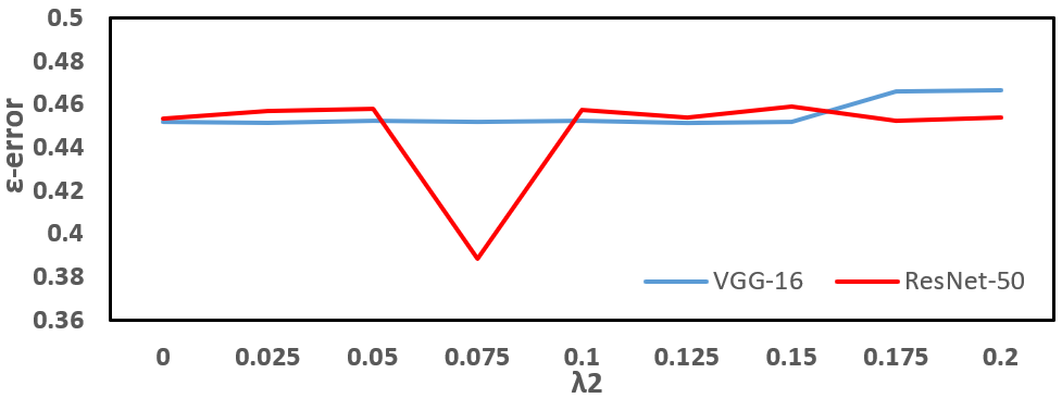
Fig. 3: The $\epsilon-$error w.r.t. $\lambda_{1}=0.2$ and $\lambda_{2}$ from 0 to 0.2.

5.5 Influences of the Parameter K

In Section 4, the influence of the choice of K on the model optimization is explained. Fig. 4 illustrates such impact of K values on the model performance. For a fixed $K$, it can be observed that the test MAE is lowest when $K=5$. Moreover, it is noted that the model with an adaptive K value consistently outperforms fixed K values. Fig. 4 describes the adaptive K values during training, which gradually converges to the best fixed K value of $5$, proving the capability of the algorithm to find the optimal $K$ during training.

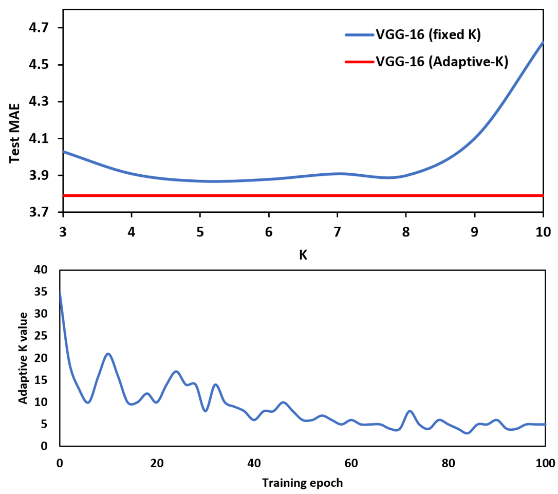
Fig. 4: Top: The MAE on FG-NET achieved by VGG-16 using different $K$ (blue line) and Adaptive-K (red line). Bottom: The adaptive $K$ value during training.

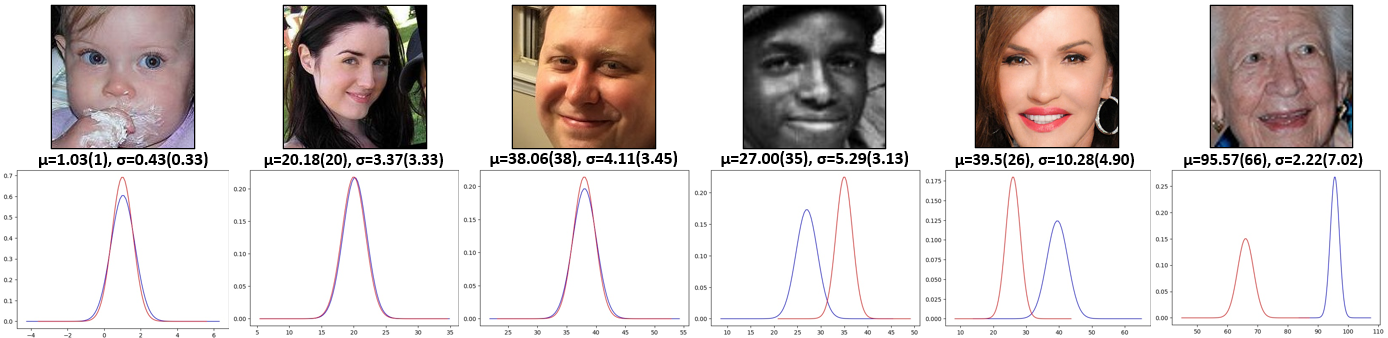
Fig. 5: Examples with age distributions ($\mu$ = ground-truth age (estimated age), $\sigma$ = ground-truth std (estimated std)) estimated by the proposed loss. The red and blue curves are the estimated and ground-truth distributions, respectively.

5.6 Comparisons with the State-of-the-art

Experiments have been carried out for comparison between the proposed method and a number of state-of-the-art benchmarks on FG-NET and CLAP2016 respectively. As indicated in Table 2, the proposed mean-residue loss achieves the lowest MAE error among these approaches in FG-NET. Experimental results show that methods with distribution learning, such as mean-variance loss [6] can outperform ranking, regression, or classification based methods [31, 4, 2]. It is noted that, in DHAA [32], a hybrid structure with multiple branches was utilized to achieve the best performance among the rest approaches. We can explore the combination of DHAA with mean-residue loss in our future work. In Table 2, we directly quote the results of DeepAge and MIPAL_SNU from [29] as a complementary comparison. Our proposed loss outperforms mean-variance loss, which proves that residue loss with adaptive-K pooling is helpful to concentrate more on top-K ages indirectly. In Fig. 5, we present some examples (3 good cases and 3 poor cases) predicted by the proposed method on CLAP $2016$. The proposed approach performs well for different age groups. But when the images have poor qualities, e.g., bad illumination, blurring, the age estimation accuracy decreases dramatically. In addition, good makeup and extreme values would influence the results.

Table 2: Comparisons of different methods

FG-NET dataset
Method	MAE	Protocol
RED-SVM [31]	5.24	LOPO
OHRank [4]	4.48	LOPO
DEX [2]	4.63	LOPO
Mean-Variance Loss [6]	3.95	LOPO
DRFs [33]	3.85	LOPO
DHAA [32]	3.72	LOPO
Adaptive Mean-Residue Loss	3.61	LOPO
CLAP2016 dataset
Method	$\varepsilon$-error	Single Model?
DeepAge [29]	0.4573	YES
MIPAL_SNU [29]	0.4565	NO
Mean-Variance Loss [6]	0.4018	YES
Adaptive Mean-Residue Loss	0.3882	YES

6 Conclusion

In this paper, we propose a simple, yet very efficient mean-residue loss for robust facial age estimation. We verify the superiority of our proposed method over state-of-the-art benchmarks through theoretical analysis and experiments. In the future, we would extend our method to other domains for continuous value estimation, such as survival year estimation in healthcare and sales prediction in e-business.

7 Acknowledgement

We are grateful for the help and support of Xiaohao Lin, Xi Fu and Ce Ju. The work is supported by Institute for Infocomm Research (I²R) and Artificial Intelligence, Analytics and Informatics (AI³), A*STAR, Singapore.

References

- [1] Yun Fu and Thomas Huang, “Human age estimation with regression on discriminative aging manifold,” IEEE Trans. Multimedia, 2008.
- [2] Z. Niu, M. Zhou, L. Wang, X. Gao, and G. Hua, “Ordinal regression with multiple output cnn for age estimation,” in IEEE CVPR, 2016.
- [3] Yixin Zhu, Jun-Yong Zhu, and Wei-Shi Zheng, “Part-based convolutional network for imbalanced age estimation,” in IEEE ICME, 2019.
- [4] Kuang-Yu Chang, Chu-Song Chen, and Yi-Ping Hung, “Ordinal hyperplanes ranker with cost sensitivities for age estimation,” in IEEE CVPR, 2011.
- [5] S. Chen, C. Zhang, M. Dong, J. Le, and M. Rao, “Using ranking-cnn for age estimation,” in IEEE CVPR, 2017.
- [6] Hongyu Pan, Hu Han, Shiguang Shan, and Xilin Chen, “Mean-variance loss for deep age estimation from a face,” in IEEE CVPR, 2018.
- [7] Karen Simonyan and Andrew Zisserman, “Very deep convolutional networks for large-scale image recognition,” arXiv preprint arXiv:1409.1556, 2014.
- [8] Zeng Zeng, Wei Zhao, Peisheng Qian, Yingjie Zhou, Ziyuan Zhao, Cen Chen, and Cuntai Guan, “Robust traffic prediction from spatial-temporal data based on conditional distribution learning,” IEEE Trans. on Cybernetics, 2021.
- [9] Young Kwon and Niels Lobo, “Age classification from facial images,” Computer Vision and Image Understanding, 1994.
- [10] Gabriel Panis, Andreas Lanitis, Nicolas Tsapatsoulis, and Timothy Cootes, “Overview of research on facial aging using the fg-net aging database,” IET Biometrics, 2015.
- [11] G. Guo, Guowang Mu, Y. Fu, and T. S. Huang, “Human age estimation using bio-inspired features,” in IEEE CVPR, 2009.
- [12] Shaoqing Ren, Kaiming He, Ross Girshick, and Jian Sun, “Faster r-cnn: Towards real-time object detection with region proposal networks,” Advances in neural information processing systems, 2015.
- [13] Yunjin Wu, Ziyuan Zhao, Shengqiang Zhang, Lulu Yao, Yan Yang, Tom ZJ Fu, and Stefan Winkler, “Interactive multi-camera soccer video analysis system,” in ACM MM, 2019.
- [14] Kaiming He, Xiangyu Zhang, Shaoqing Ren, and Jian Sun, “Deep residual learning for image recognition,” in IEEE CVPR, 2015.
- [15] Peisheng Qian, Ziyuan Zhao, Haobing Liu, Yingcai Wang, Yu Peng, Sheng Hu, Jing Zhang, Yue Deng, and Zeng Zeng, “Multi-target deep learning for algal detection and classification,” in IEEE EMBC, 2020.
- [16] Xiaodong Qu, Qingtian Mei, Peiyan Liu, and Timothy Hickey, “Using eeg to distinguish between writing and typing for the same cognitive task,” in International Conference on Brain Function Assessment in Learning. Springer, 2020.
- [17] Xiaodong Qu, Peiyan Liu, Zhaonan Li, and Timothy Hickey, “Multi-class time continuity voting for eeg classification,” in International Conference on Brain Function Assessment in Learning. Springer, 2020.
- [18] Yi Ding, Nigel Wei Jun Ang, Aung Aung Phyo Wai, and Cuntai Guan, “Learning generalized representations of eeg between multiple cognitive attention tasks,” in IEEE EMBC, 2021.
- [19] Steven Yi, Minta Lu, Adam Yee, John Harmon, Frank Meng, and Saurabh Hinduja, “Enhance wound healing monitoring through a thermal imaging based smartphone app,” in Medical Imaging 2018: Imaging Informatics for Healthcare, Research, and Applications, 2018.
- [20] Ziyuan Zhao, Zeng Zeng, Kaixin Xu, Cen Chen, and Cuntai Guan, “Dsal: Deeply supervised active learning from strong and weak labelers for biomedical image segmentation,” IEEE Journal of Biomedical and Health Informatics, 2021.
- [21] Ziyuan Zhao, Kaixin Xu, Shumeng Li, Zeng Zeng, and Cuntai Guan, “Mt-uda: Towards unsupervised cross-modality medical image segmentation with limited source labels,” in MICCAI. Springer, 2021.
- [22] Dong Yi, Zhen Lei, and Stan Z. Li, “Age estimation by multi-scale convolutional network,” in ACCV, 2015.
- [23] F. Wang, H. Han, S. Shan, and X. Chen, “Deep multi-task learning for joint prediction of heterogeneous face attributes,” in IEEE International Conference on Automatic Face Gesture Recognition, 2017.
- [24] Xusheng Zeng, Junyang Huang, and Changxing Ding, “Soft-ranking label encoding for robust facial age estimation,” IEEE Access, 2020.
- [25] X. Geng, “Label distribution learning,” IEEE Trans. on Knowledge and Data Engineering, 2016.
- [26] Zhouzhou He, Xi Li, Zhongfei Zhang, Fei Wu, Xin Geng, Yaqing Zhang, Ming-Hsuan Yang, and Yueting Zhuang, “Data-dependent label distribution learning for age estimation,” IEEE Tran. on Image Processing, 2017.
- [27] Xin Geng, Chao Yin, and Zhi-Hua Zhou, “Facial age estimation by learning from label distributions,” IEEE Trans. Pattern Anal. Mach. Intell., 2013.
- [28] Gabriel Panis and Andreas Lanitis, “An overview of research activities in facial age estimation using the fg-net aging database,” in ECCV. Springer, 2014.
- [29] Sergio Escalera, Mercedes Torres Torres, Brais Martinez, Xavier Baró, Hugo Jair Escalante, Isabelle Guyon, Georgios Tzimiropoulos, Ciprian Corneou, Marc Oliu, Mohammad Ali Bagheri, et al., “Chalearn looking at people and faces of the world: Face analysis workshop and challenge 2016,” in IEEE CVPRW, 2016.
- [30] Olga Russakovsky, Jia Deng, Hao Su, Jonathan Krause, Sanjeev Satheesh, Sean Ma, Zhiheng Huang, Andrej Karpathy, Aditya Khosla, Michael Bernstein, et al., “Imagenet large scale visual recognition challenge,” International journal of computer vision, 2015.
- [31] Kuang-Yu Chang, Chu-Song Chen, and Yi-Ping Hung, “A ranking approach for human ages estimation based on face images,” in IEEE CVPR, 2010.
- [32] Zichang Tan, Yang Yang, Jun Wan, Guodong Guo, and Stan Z. Li, “Deeply-learned hybrid representations for facial age estimation,” in IJCAI, 2019.
- [33] W. Shen, Y. Guo, Y. Wang, K. Zhao, B. Wang, and A. Yuille, “Deep regression forests for age estimation,” in IEEE CVPR, 2018, pp. 2304–2313.