Predicting extreme events from data using deep machine learning: when and where

Abstract

We develop a deep convolutional neural network (DCNN) based framework for model-free prediction of the occurrence of extreme events both in time (“when”) and in space (“where”) in nonlinear physical systems of spatial dimension two. The measurements or data are a set of two-dimensional snapshots or images. For a desired time horizon of prediction, a proper labeling scheme can be designated to enable successful training of the DCNN and subsequent prediction of extreme events in time. Given that an extreme event has been predicted to occur within the time horizon, a space-based labeling scheme can be applied to predict, within certain resolution, the location at which the event will occur. We use synthetic data from the 2D complex Ginzburg-Landau equation and empirical wind speed data of the North Atlantic ocean to demonstrate and validate our machine-learning based prediction framework. The trade-offs among the prediction horizon, spatial resolution, and accuracy are illustrated, and the detrimental effect of spatially biased occurrence of extreme event on prediction accuracy is discussed. The deep learning framework is viable for predicting extreme events in the real world.

I Introduction

One of the outstanding and most challenging problems in nonlinear dynamics and complex systems is predicting extreme events in spatiotemporal chaotic systems. Extreme events, also known as rare and intense events, occur in a variety of physical systems [1]. Familiar examples include earthquakes, intense tropical cyclones, tornadoes, and rogue ocean waves. For example, rough waves in the ocean can arise from long-range acoustic wave propagation through ocean’s sound channel [2]. In optics (e.g., optical fiber systems), extreme events can manifest themselves as waves with an abnormally large amplitude - rogue waves [3, 4, 5]. Extreme events can also occur in engineering systems, e.g., complex networked or online systems, examples of which range from sudden bursts of packet flows on the internet, jamming in computer or transportation networks, denial-of-service cyberattacks, and blackouts due to load imbalances in the electrical power grid. There have been efforts in statistical characterization of extreme events and in understanding their dynamical origin [1, 6, 7, 8, 9, 10, 11, 12, 13, 14, 15, 16, 17]. For example, the statistical distribution [6] and the recurrent or long-term correlation property [8, 10] of extreme events were studied. There were also efforts in predictability [18, 19, 20, 21] and model-based control [22, 23, 24] of extreme events. Catastrophic events in the past two decades include the crash of China Airlines Flight 611 due to metal fatigue in 2002, the Fukushima Daiichi nuclear plant meltdown due to a tsunami wave triggering boiling water reactors shutdown in 2011, and hurricane Harvey in the Gulf of Mexico in 2017 that took away the lives of more than 100 people and caused $125 billion damage [25]. Due to global-warming induced climate change [26], extreme events are likely to occur at an increasingly high frequency with severe social, environmental and economical damages [27, 28, 29, 30, 31]. While there have been recent efforts in model based prediction of extreme events [32, 33], in realistic situations, an accurate model underlying the dynamical process leading to an extreme event often is not available. It is imperative to develop model-free prediction methods based solely on data. This problem, despite its paramount importance, has remained outstanding.

In this paper, we develop a deep machine learning framework to predict extreme events without requiring any model of the underlying system. Recent years have witnessed tremendous development in machine learning, especially various deep learning methods [34, 35, 36, 37] based on artificial neural networks, with applications in a wide variety of areas. For example, deep learning has been used to recognize speech and visual objects [38, 39, 37], to predict the potential structure-activity relationships among drug molecules [40], to detect major depressive disorder from EEG signals [41], and even to beat the human player in Go game [42]. On predicting severe weather and climate events, methods based on artificial neural networks or artificial intelligence have been deemed important and potentially feasible [25, 43]. For example, deep convolutional neural networks (DCNNs) have been used to predict the EI Niño/South Oscillations [44] that occur over a much longer time scale (e.g., months or a year) than those of extreme weather events such as intense tropical cyclones (e.g., days or weeks). A binary classification scheme was formulated for deriving optimal predictors of extremes directly from data [45]. More recently, a densely connected mixed-scale network model was proposed [46] to predict extreme events in the truncated Korteweg–de Vries equation - a nonlinear partial differential equation (PDE) in one spatial dimension which describes the complex dynamics in surface water wave turbulence. Our focus here is on DCNN based prediction of extreme events in terms of the “when” and “where” issues using synthetic data from spatiotemporal nonlinear dynamical systems and empirical image data from a real atmospheric system.

We consider the setting of a two-dimensional (2D) closed domain in which extreme events occur. This setting is quite ubiquitous for studying extreme events in the natural world, such as earthquakes that occur in a finite geophysical area or extreme wind speed in an oceanic region. Physically, the extreme events represent exceptionally high amplitude or intensity of some “field” such as the seismological wave or the velocity field of the wind across a specific spatial region. For simplicity, we consider a square 2D domain in which extreme events occur randomly in both space and time. If we color-code the amplitude or intensity of the field, its distribution at any instant of time is effectively an image - a snapshot. An extreme event at some instant of time will manifest itself as a bright spot somewhere in the image. As the system evolves in time, a large number of snapshots of the field distribution in the spatial domain can be taken. Some of these snapshots or images may contain an extreme event, while many others may not. Properly labeled images serve naturally as inputs to a DCNN for training and prediction.

We exploit DCNN to predict extreme events, focusing on the critical questions of “when” and “where,” i.e., when and where in the region of interest do extreme events occur? To address the “when” question, we distinguish or label the instantaneous state distribution of the system (the images) into two classes: one in an appropriate time interval preceding the occurrence of an extreme event (e.g., labeled as 1) and another with no extreme event in the next time interval of the same length (labeled as 0). We then train a DCNN with a large number of randomly mixed labeled images. After successful completion of training, the DCNN possesses the predictive power in that, when a new image is presented to it, the deep networked system can output the correct label with reasonable accuracy, effectively solving the “when” problem by predicting whether an extreme event is going to occur in the next time interval. The initially pre-defined time interval is thus the time horizon of prediction. Given that an extreme event has been predicted to occur within the horizon, we can address the “where” question by focusing on the images that carry a 1 label. In particular, we divide the spatial domain into a grid of cells of equal area. For example, for a $4\times 4$ grid, each cell carries a label, e.g., from 0 to 15. If the extreme event occurs in one of the cells, e.g., cell 12, then this image carries the label 12, and so on. This way, the available images are partitioned into 16 classes, and the DCNN can be trained with a large number of such labeled images for gaining the power to predict in which spatial cell would an extreme event occur, effectively solving the “where” problem. The size of each cell determines the spatial resolution of prediction. There are trade-offs among the three key indicators: the time horizon, the spatial resolution, and the prediction accuracy. In general, increasing the prediction horizon or the spatial resolution or both will reduce the accuracy.

Taken together, our DCNN based prediction paradigm consists of two steps. Firstly, we predict whether an extreme event would occur in a given time interval in the future (the “when” problem). Secondly, given that an extreme event is going to occur within the time horizon, we predict the location of the event with certain spatial resolution (the “where” problem). For illustration, we use synthetic data from a model and empirical data from a real atmospheric system: the 2D complex Ginzburg-Landau equation (CGLE) and the wind speed distribution in the North Atlantic ocean. In each case, we quantify the prediction results, demonstrate that reasonably high prediction accuracy can be achieved, and discuss the trade-offs among the time horizon, spatial resolution, and prediction accuracy.

II Results

We choose two classic and widely used DCNNs to predict extreme events in spatiotemporal dynamical systems: LeNet-5 [47] and ResNet-50 [37]. LeNet-5 was first articulated for classification of handwritten characters in 1998, and it has inspired the development of state-of-the-art DCNNs for tasks such as image recognition [38], image segmentation [48], and object detection [49]. The DCNN ResNet-50, a much “deeper” neural network in that it has substantially more hidden layers than LeNet-5, was developed in 2016, where a residual learning framework was introduced to expedite training (ResNet was the winner of the ILSVRC 2015 classification task). We shall demonstrate that both LeNet-5 and ResNet-50 have the power to predict extreme events.

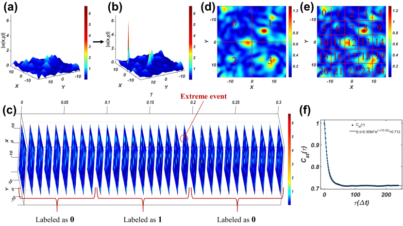
Figure 1: Representative 2D states of CGLE without or with an extreme event and an example of training data labeling scheme for DCNN. (a) A 2D state without any extreme event and (b) a state with an extreme event that occurs ten time steps after the state in (a), where an extreme event is defined if the maximum magnitude of the instantaneous amplitude in space exceeds the threshold value $|\bar{u}|=5$. (c) A sequence of 31 snapshots that occur consecutively in time (total time duration $=0.3$), separated by time step $\Delta t$, together with a labeling scheme for predicting “when” an extreme event will occur, where the state with an extreme event and all preceding $p=10$ states are labeled as ${\bf 1}$, and all other states are labeled as ${\bf 0}$. The time horizon of prediction is $p\Delta t$. In general, there is a trade-off between the prediction horizon and accuracy. (d) A labeling scheme for predicting the location of the occurrence of the extreme event, where the entire domain is divided into a $2\times 2$ grid with the four cells labeled as ${\bf 0}$, ${\bf 1}$, ${\bf 2}$, and ${\bf 3}$, respectively. The color coding is based on the magnitude $|u|$ of the complex field. (e) A finer labeling scheme by which the domain is divided into a $5\times 5$ grid, generating 25 classes of images. There is a trade-off between spatial resolution and prediction accuracy as well. (f) Temporal correlation function $C_{st}(\tau)$ of 2D CGLE system, where the black dots and the blue curve are the actual correlation function and the exponential fitting. The time constant $\tau_{c}$ is about $10.33$. (See Appendix A for the definition of $C_{st}(\tau)$ and the simulation setting.)

II.1 Predicting extreme events based on synthetic data from a paradigmatic model of nonlinear physical systems

To test and demonstrate the power of DCNNs to predict extreme events in a controlled setting, we exploit a general mathematical model of diverse physical systems to generate synthetic datasets. In particular, we consider a finite 2D domain in which a set of physical variables evolve according to nonlinear dynamical rules and extreme events occur infrequently at different locations from time to time. From a dynamical systems point of view, extreme events are the consequence of the nonlinear interactions among different components of the system and are typically due to constructive interference among these components. For example, in a wave system, the wave amplitude at a spatial location at any time is the result of the superposition of many wave packets at different spatial locations from some earlier time. If the phases of most wave packets become coherent at certain time instant, a large amplitude event can arise at this moment. Phase coherence, however, is rare, and so are extreme wave events. Mathematically, it is convenient to describe the system by nonlinear PDEs in spatial dimension two. Because of nonlinearity, sensitive dependence on initial conditions, parameter fluctuations or external perturbations can arise. As a result, extreme events can occur throughout the domain at random time and locations. The general setting describes real-world phenomena such as material failures for which two-dimensional images can be obtained or earthquakes in a geographical region.

To be concrete, we study a closed PDE system of spatial dimension two as described by the CGLE (Appendix A), which is a paradigmatic model for gaining insights into a variety of physical phenomena such as nonlinear waves in optical fibers, chemical reactions, superconductivity, superfluidity, Bose-Einstein condensation, and liquid crystals [50, 51, 52]. Figures 1(a) and 1(b) show two representative snapshots of the amplitude distribution of the complex field $u(x,y)$ at two instants of time, one without and another with an extreme event as indicated by the localized, high-amplitude peak, respectively, where the former occurs ten time steps before the latter. A close examination of the 2D state in Fig. 1(a) gives no indication that an extreme event is going to occur in the near future, let alone its spatial location.

To enable a DCNN to predict extreme events in both time and space, an essential step is to articulate proper labeling schemes for the 2D states. Figure 1(c) illustrates a labeling scheme for predicting when an extreme event will occur, where all prior 2D states within $p$ time steps of the occurrence of an extreme event (including the 2D state containing the event) are labeled as ${\bf 1}$, and all other 2D states are labeled as ${\bf 0}$. In general, the value of $p$ determines the prediction horizon and accuracy, and the trade-off between them provides a criterion for choosing $p$. To see this, it is convenient to use the mean temporal period or the time constant $\tau_{c}$ underlying the temporal correlation function of the state evolution as a reference time scale. For $p<\tau_{c}$, the prediction horizon is short, but the 2D states labeled as ${\bf 1}$ are highly correlated with the state containing the extreme event, making it possible to achieve a high prediction accuracy. However, for $p>\tau_{c}$, the prediction horizon is long but the accuracy will be sacrificed. Empirically, a proper choice of $p$ is $p\approx\tau_{c}$. In Fig. 1(c), we have $p=10$.

Given that an extreme event has been predicted to occur within $p$ time steps, we can predict its location by dividing the entire 2D domain into a uniform grid with a distinct label for each cell. For example, in Fig. 1(d) where the 2D state is the same as that in Fig. 1(a), the spatial domain is divided into a $2\times 2$ grid with four cells labeled as ${\bf 0}$, ${\bf 1}$, ${\bf 2}$, and ${\bf 3}$, respectively, where a specific label indicates the cell in which the extreme event will occur. Alternatively, a higher spatial resolution can be used, as shown in Fig. 1(e), where the domain is divided into a $5\times 5$ grid. As we will demonstrate, there is a trade-off between spatial resolution and prediction accuracy: a higher resolution generally reduces the accuracy.

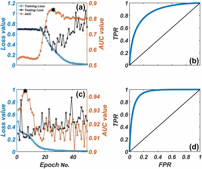
Figure 2: Predicting occurrence of an extreme event with DCNN - the issue of “when”. Two types of DCNNs are used: LeNet-5 and ResNet-50. (a) With LeNet-5, training loss (blue circles), testing loss (black squares), and AUC value (brown diamonds) versus the number of training epochs. The black hexagram marker represents the epoch at which the best AUC value is achieved. (b) The ROC curve corresponding to the black hexagram in (a). (c) Results similar to those in (a) but from ResNet-50, with the same legends as in (a). (d) The ROC curve corresponding to the black hexagram in (c). The amplitude threshold for defining an extreme event is $|\bar{u}|=5$.

We now address the “when” question, i.e., to predict the possible occurrence of an extreme event within a reasonable time interval in the future. Because of our labeling scheme to associate an extreme event with $p$ snapshots of 2D states prior to or at its occurrence, the prediction horizon is $p$ time steps, i.e., $p\Delta t$, where $\Delta t$ is the sampling time interval. Ideally, after training is completed, the DCNN should be able to give a label, either ${\bf 0}$ or ${\bf 1}$, to any snapshot of the system state in space during its course of evolution. At a given time with a specific snapshot as input, if the DCNN outputs label ${\bf 1}$, an extreme event is predicted to occur within the next $p$ time steps, with uncertainty determined by the prediction accuracy. If the output label is deemed to be ${\bf 0}$, there will be no extreme event within the prediction horizon counted from the present time.

To quantify the performance of the DCNN for predicting when an extreme event would occur, we use the receiver operating characteristic (ROC). A ROC curve is generated with the true-positive rate (TPR) and the false-positive rate (FPR) on the Y and X-axis, respectively. The best possible performance corresponds to the top left corner (TPR = 1 and FPR = 0), so the area under the ROC curve (AUC) is one - the maximally possible value. In general, large AUC values indicate a better performance. (A detailed description of how the ROC curve is calculated can be found in Appendix B.)

Figure 2 presents a representative example for predicting extreme events in the CGLE, where one training dataset has $100007$ 2D states, out of which $50006$ and $50001$ 2D states are labeled as ${\bf 1}$ and ${\bf 0}$, respectively. A larger dataset is also tested, which contains $224010$ 2D states with $15800$ and $208210$ states labeled as ${\bf 1}$ and ${\bf 0}$, respectively. (A detailed description of how the training datasets are generated can be found in Appendix A.) Figures 2(a) and 2(c) show the loss values and the AUC for training and testing with LeNet-5 and ResNet-50, respectively. Both DCNNs are trained using the deep learning framework Pytorch [53, 54], with binary cross-entropy loss function and a stochastic gradient descent optimizer. The relevant parameters are: batch size 128, learning rate $10^{-3}$, momentum factor 0.9, and L2 penalty $5\times 10^{-4}$ (see description in SI - Supporting Information [55]). From Fig. 2(a), we see that, for LeNet-5, the training loss starts to decrease steadily at about the $20$th training epoch, after which the training loss keeps decreasing as the number of training epochs is increased, but the testing loss decreases initially and then starts to increase slowly. For the test dataset, the best AUC value (about 0.857, marked as a black hexagram) is achieved at about the $26$th epoch. Figure 2(b) shows the corresponding ROC curve for LeNet-5. While the ROC curve involves a series of systematically varying threshold values for distinguishing the two output labels, a natural choice is $0.5$, i.e., an output value larger or smaller than $0.5$ represents prediction of class ${\bf 1}$ or ${\bf 0}$, respectively. For this choice of the threshold, the numbers of true-positive, false-positive, false-negative, and true-negative cases are $N_{TP}=11501$, $N_{FP}=37141$, $N_{FN}=4299$ and $N_{TN}=171069$, respectively, so the values of $\mbox{TPR}\equiv N_{TP}/(N_{TP}+N_{FN})$ and $\mbox{FPR}\equiv N_{FP}/(N_{FP}+N_{TN})$ are $72.79\%$ and $17.84\%$, respectively. For LeNet-5, the overall prediction accuracy is approximately $81.5\%$. The corresponding results for ResNet-50 are shown in Figs. 2(c) and 2(d). We see that only six training epochs are necessary to achieve the best performance with $\mbox{AUC}\approx 94.4\%$ (the prediction accuracy), after which the training loss decreases gradually as the number of training epochs is increased. However, there are fluctuations associated with the testing loss. The ROC curve corresponding to the best AUC value is shown in Fig 2(d). For the threshold value $0.5$, the numbers of true-positive, false-positive, false-negative, and true-negative cases are $12930$, $19742$, $2870$, and $188468$, respectively, giving the values of TPR and FPR as $81.84\%$ and $9.48\%$, respectively.

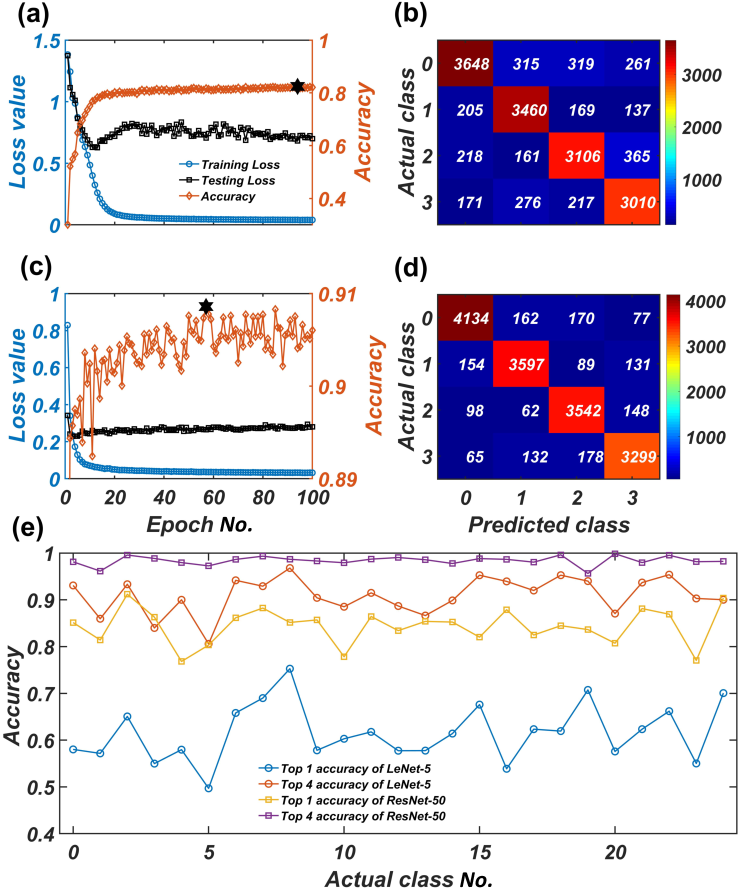
Figure 3: Predicting the occurrence of an extreme event with DCNN - the issue of “where”. Given that an extreme event has been predicted to occur within $p$ time steps in the future, a labeling scheme based on a uniform spatial grid can be used to train the DCNNs. (a) For LeNet-5, training loss (blue circles), testing loss (black squares), and accuracy (brown diamonds) versus the length of the training phase, where the black hexagram marker represents the training epoch at which the best accuracy is achieved. (b) The confusion matrix associated with the black hexagram in (a). (c,d) Results corresponding to those in (a,b), respectively, but for ResNet-50. In (a-d), the spatial domain is divided into a $2\times 2$ grid. (e) For both LeNet-5 and ResNet-50 with a $5\times 5$ division of the domain, the top-one (one cell) and top-four (four cells with the highest accuracy values combined) accuracy for each class for predicting where the extreme will occur in the domain. For ResNet-50, the top-four accuracy is better than $95\%$. The amplitude threshold for defining an extreme event is $|\bar{u}|=5$.

Having used DCNN to predict that an extreme event will occur in the next $p$ time steps, it is necessary to predict where it will occur in the spatial domain of interest. Here we demonstrate that this “where” issue can be addressed using DCNNs as well. Specifically, we use an independent DCNN and carry out the training beforehand, as follows. We gather all the state snapshots carrying the label ${\bf 1}$ from the original dataset. Take the case in Fig. 2 as an example. The original dataset contains $50006$ such 2D states. If we divide the space into four identical subcells with the labels ${\bf 0}$, ${\bf 1}$, ${\bf 2}$, and ${\bf 3}$, the respective numbers of snapshots are $12628$, $12870$, $12320$, and $12188$. Note that these numbers are approximately the same, indicating that the dataset is unbiased in the space in the sense that the probability for an extreme even to occur is roughly uniform across the entire domain. The whole dataset is divided into a training dataset of $33968$ and a testing dataset of $16038$ snapshots. In the testing set, there are $4543$, $3971$, $3850$, and $3674$ 2D states that are labeled as class ${\bf 0}$, ${\bf 1}$, ${\bf 2}$, and ${\bf 3}$, respectively. Figures 3(a) and 3(c) show the loss and accuracy values during the training of DCNN LeNet-5 and ResNet-50, respectively, where the accuracy is calculated based on the whole testing dataset, i.e., with respect to all four classes. As for the case of predicting when an extreme event will occur, both DCNNs are trained using the deep learning framework Pytorch [53, 54] with the same training parameter values as those in Fig. 2. At the beginning of the training phase, the values of testing loss and accuracy change quite rapidly. However, after several training epochs, both types of DCNNs have attained stable testing loss and accuracy. For LeNet-5 and ResNet-50, optimal training with the highest accuracy is achieved at epoch $94$ and $57$, respectively. (Note that the best accuracy does not correspond to the lowest testing loss.) Figures 3(b) and 3(d) present the confusion matrices of the predicted class versus the actual class for the testing result of the best accuracy for LeNet-5 and ResNet-50, respectively, where the values of the diagonal elements indicate correct prediction while those of off-diagonal elements represent errors. We see that the diagonal elements are much larger than the off-diagonal elements, suggesting the effectiveness of prediction. For LeNet-5, the prediction accuracy for classes ${\bf 0}$, ${\bf 1}$, ${\bf 2}$, and ${\bf 3}$ are approximately $80.30\%$, $87.13\%$, $80.68\%$ and $81.93\%$, respectively, while the respective accuracy values for ResNet-50 are higher: $91.00\%$, $90.58\%$, $92.00\%$, and $89.79\%$.

We have also tested a spatial grid of higher resolution: $5\times 5$. In this case, there are 25 labels, corresponding to 25 training classes. The prediction accuracy for all classes is shown in Fig. 3(e) for both LeNet-5 and ResNet-50. During prediction, for any input image, the output of the DCNN is a $25\times 1$ vector, each element of which gives the respective probability for each predicted class. Two types of accuracy are calculated: top-1 accuracy, which is simply the prediction accuracy for each class, and top-4 accuracy, which for each class is defined as the accuracy of predicting the occurrence of the extreme event in the four cells with the highest predicted probability values. If such four cells contain the actual class, the top-four accuracy would be $100\%$; otherwise, it is zero. Averaging over all images of the specific class gives the top-four accuracy value, as shown in Fig. 3(e). We have that the average values of the top-one accuracy for LeNet-5 and ResNet-50 are approximately $61.49\%$ and $84.34\%$, respectively, indicating that ResNet-50 is more effective at predicting the location of occurrence of the extreme event. The mean top-4 accuracy achieved with ResNet-50 is remarkably high: $98.37\%$. (The corresponding confusion matrix is presented in SI [55].)

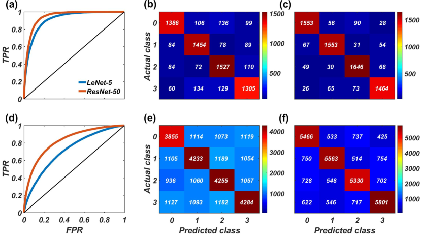
Figure 4: Performance robustness of DCNN based prediction of extreme events in terms of occurrence time and spatial location in CGLE. (a-c) ROC curves and confusion matrices for the same dataset as in Figs. 2 and 3 but with the threshold $|\bar{u}|$ in the amplitude for defining an extreme event increased from 5 to 6, for $p=10$. (d-f) ROC curves and confusion matrices for $|\bar{u}|=5$ and $p=20$. In (a) and (d), the best ROC curves for LeNet-5 and ResNet-50 are presented, respectively. Panel pairs (b,e) and (c, f) show the corresponding confusion matrices for LeNet-5 and ResNet-50, respectively.

To demonstrate the robustness of DCNN based prediction of extreme events, we study the performance characteristics for different values of the amplitude threshold $|\bar{u}|$ for defining an extreme event. Figure 4(a) show, for the same data set as in Figs. 2 and 3, results for predicting “when” an extreme event will occur for $|u|=6$. Because of the higher amplitude threshold value, the number of states labeled as ${\bf 1}$ is smaller: in this case there are $6780$ and $217230$ 2D states labeled as ${\bf 1}$ and ${\bf 0}$ in the dataset, respectively. What is displayed in Fig. 4(a) is the best ROC curves for LeNet-5 and ResNet-50, where the corresponding AUC values are approximately $0.91$ and $0.94$, respectively. Comparing Fig. 4(a) with Figs. 2(b) and 2(d), we see that a small increase in the amplitude threshold value improves the performance of LeNet-5 but that of ResNet-50 is largely unaffected. The fact that the AUC values are above 0.9 indicates robust predictability of both types of DCNNs for extreme events. Figure 4(b) shows the corresponding confusion matrix for LeNet-5 for predicting “where” the extreme event, which has been predicted to occur within the time horizon [as characterized by Fig. 4(a)], will occur, where the spatial domain is divided into a $2\times 2$ grid with four spatial labels (classes) to be predicted. The prediction accuracies for the extreme event to occur in the four subdomains (classes ${\bf 0}$ to ${\bf 3}$) are approximately $80.25\%$, $85.28\%$, $85.16\%$, and $80.16\%$, respectively. The corresponding results for ResNet-50 are shown in Fig. 4(c), where the prediction accuracies for classes ${\bf 0}$ to ${\bf 3}$ are approximately $89.92\%$, $91.09\%$, $91.80\%$, and $89.93\%$, respectively. Comparing the results in Figs. 4(b) and 4(c) with those in Figs. 3(b) and 3(d), we observe a similar level of prediction accuracy, indicating that changing the amplitude threshold for extreme events has little effect on predictability.

Will modifying the labeling time duration parameter $p$ for extreme event have any effect on the predictability? To address this question, we double the value of $p$ in Figs. 2 and 3 from $10$ to $20$, so the prediction time horizon is now twice as long. In this case, there are $28524$ and $195486$ state images labeled as ${\bf 1}$ and ${\bf 0}$, respectively, where the number of states labeled as ${\bf 1}$ is larger due to the larger value of $p$. Figure 4(d) shows the best ROC curves obtained from LeNet-5 and ResNet-50, where the respective AUC values are approximately $0.72$ and $0.82$. Comparing with the corresponding results in Figs. 2(b) and 2(d), we see that a larger $p$ value tends to degrade the predictability of both types of DCNNs. This is intuitively expected: the time horizon of prediction can be increased but at the price of sacrificing accuracy. However, despite the decrease in accuracy, the AUC values for both cases are still much larger than $0.5$. Accuracy deterioration not only occurs in the time horizon of prediction, it is also reflected in the accuracy of prediction of the occurrence of the event in space. Figure 4(e) shows, for LeNet-5, the confusion matrix for predicting “where” the extreme event will occur in one of the four subdomains, where the prediction accuracies for the four classes are approximately $53.8\%$, $55.8\%$, $58.2\%$, and $55.7\%$, respectively, which are lower than the corresponding values in Fig. 3(b). The results for ResNet-50 is shown Fig. 4(f), where the prediction accuracies of the four classes are approximately $76.3\%$, $73.4\%$, $72.9\%$, and $75.5\%$, respectively, which are somewhat lower than the corresponding accuracy values in Fig. 3(d). Overall, even with a doubly stretched prediction time horizon, both types of DCNNs are still capable of predicting “when” and “where” an extreme event will occur with reasonable accuracy, with the larger and deeper ResNet-50 superior to LeNet-5 in terms of performance. [Detailed results (e.g., loss curves, ROC curves, AUC values, and confusion matrices) with a finer spatial grid ($5\times 5$ with 25 subdomains or classes) are presented in SI [55].]

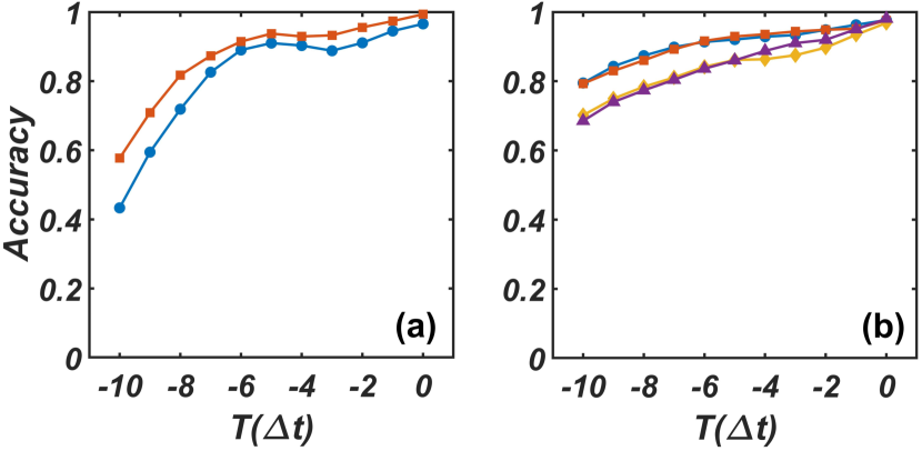
Figure 5: The “when” and “where” prediction accuracy at a series of time steps preceding the occurrence of an extreme event. In both panels, the abscissa denotes the time step relative to the extreme event that occurs at time zero. For example, $-10$ means ten steps prior to the event. In (a) where the prediction scenario is “when,” the blue and brown curves represent the prediction accuracy at each time step for $|\bar{u}|=5.0$ and $|\bar{u}|=6.0$, respectively. The threshold used in calculating the ROC curve is 0.5. In (b), the prediction scenario is “where,” in which the blue, brown, yellow, and purple curves represent the cases of a $2\times 2$ spatial grid with $|\bar{u}|=5$, a $2\times 2$ grid $|\bar{u}|=6$, a $5\times 5$ grid with $|\bar{u}|=5$, and a $5\times 5$ grid with $|\bar{u}|=6$, respectively. The prediction horizon is $p=10$, and the DCNNs are of the ResNet-50 type. The models for the results in panel (a) is the one in Figs. 2(d) and 4(a). For (b) the model is the one in Figs. 3(d),  4(c), Fig. S3, and Fig. S5.

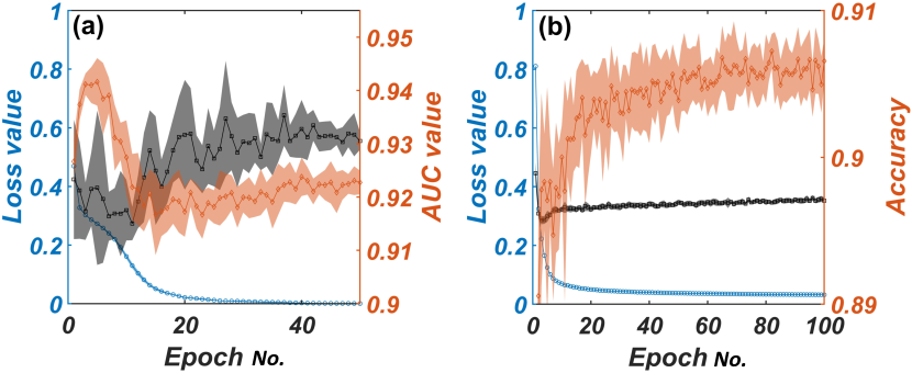
Figure 6: Ensemble average of training loss, testing loss, AUC value, and accuracy for the “when” and “where” problems. (a,b) Results for the setting in Figs. 2(c) and 3(c), respectively. In (a), the blue, black, and brown traces correspond to the ensemble average of training loss, testing loss, and AUC value, respectively. The shadowed region about each line is within the standard deviation. In (b), the blue, black, and brown traces correspond to the ensemble average of training loss, testing loss, and accuracy, respectively.

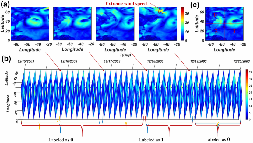
Figure 7: Image data of wind speed in the North Atlantic ocean and labeling schemes for DCNN. (a) Four representative images of the wind speed in the North Atlantic ocean and (b) a stack of wind speed images from December 15 to 20, 2003. In (a), the horizontal and vertical axes are the west longitude and north latitude, respectively, and the time instants that the four states occur are marked in (b). Three labeling schemes for using DCNNs to predict “when” an event of extreme wind speed will occur are specified in (b). (c) A labeling scheme for predicting “where” an extreme event will occur.

To assess the performance of DCNN within the horizon of predicting “when” and “where” an extreme event would occur, we calculate the accuracy at each time step within the prediction horizon, as shown in Figs. 5(a) and  5(b), respectively. In particular, Fig. 5(a) shows that, ten time steps prior to the occurrence of the extreme event, the prediction accuracy is the lowest. This is expected because the earlier to start prediction, less is the information about the extreme event. At this time, for $|\bar{u}|=6$, the prediction accuracy is about $60\%$, which is already above the $50\%$ random level. Moving closer to the event, the prediction accuracy tends to increase toward $100\%$. For example, at seven time steps before the extreme event, the accuracy exceeds $80\%$ for both $|\bar{u}|=5$ and $|\bar{u}|=6$ cases. Figure 5(b) shows the accuracy of predicting “where” an extreme event will occur at each time step within the prediction horizon. For the two cases of partitioning the domain into $4$ subregions, the prediction accuracy is at or above the $80\%$ level at each time step. For the two cases of $25$ subregions, the overall prediction accuracy is reduced slightly but it is still at or above the $70\%$ level for each time step. Figure 5 thus demonstrates that DCNNs are capable of predicting “when” and “where” an extreme event will occur within the prediction horizon.

To test the stability of our DCNN prediction method, we take the 2D CGLE system and produce ten random realizations of the training and test using the same settings as in Figs. 2(c) and 3(c). Figures 6(a) and 6(b) show the ensemble average of training loss, testing loss, the AUC value, and the prediction accuracy for the settings of Figs. 2(c) and 3(c), respectively. It can be seen that all ten realizations of the training loss, testing loss, AUC value, and accuracy exhibit the same trend. For example, when using ResNet-50 to predict “when” an extreme event would occur, the largest AUC value is achieved at about five epochs, as shown in Fig. 6(a). When predicting the location of the extreme event, the prediction accuracy approaches a constant value as more training epochs are used, as shown in Fig. 6(b). The largest average prediction accuracy occurs at about the $82$nd epoch. Therefore, within 100 training epochs, there is little over-fitting, demonstrating that the DCNN is able to generate stable and accurate prediction results.

II.2 Predicting the occurrence of extreme wind speed in North Atlantic ocean based on real-world data

We test the power of DCNNs to predict extreme events in the real world. Our concrete example is to predict the extreme wind speed in the North Atlantic ocean from real datasets (described in Appendix C). Figure 7(a) shows four typical wind speed images, where an extreme event of wind speed greater than $30$m/s occurs towards the northern part in the rightmost image as indicated and the three images from left to right represent the data three days, two days, and one day before the occurrence of the extreme event, respectively. The occurrence time of the four data images is indicated in Fig. 7(b). Three possible labeling schemes for a DCNN to predict “when” an extreme event will occur are specified in Fig. 7(b) by the red, blue and yellow brackets, in which the data one, two, and three days prior to the occurrence of the extreme event are labeled as ${\bf 1}$, corresponding to a prediction horizon of one, two, and three days, respectively. For convenience, we call the three corresponding labeling schemes as 3DLS, 2DLS, and 1DLS. In general, setting a longer horizon leads to reduced prediction accuracy. (The label shown in Fig. 7(b) is only related to the extreme wind event in  7(a). The actual label scheme takes into account the situation where two extreme events occur in the same prediction horizon. The time evolution of the maximum wind speed is shown in Fig. S1 in Supporting Information. Figure 7(c) depicts a labeling scheme for predicting “where” the extreme event will occur, after it has been predicted to occur within a specific time horizon, where the spatial domain of interest is divided into $4$ sub-domains with distinctive labels, leading to $4$ classes to be trained and predicted.

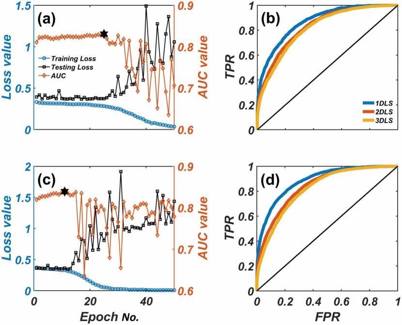
Figure 8: DCNN based prediction of “when” an extreme wind speed will occur. (a,b) Losses, AUC value, and ROC curves for the dataset restructured from the original data with time step $\Delta t=6$ hours. (c,d) The same quantities as those in (a,b) but for the forecast dataset with time step $\Delta t=3$ hours. In (a,c), training and testing losses as well as changes in the AUC value are plotted with the increase of training epochs for 2DLS. (b,d) The ROC curves for the three distinct labeling schemes specified in Fig. 7(b). In all cases, the DCNN is ResNet-50 and the threshold value of the wind speed for defining an extreme event is set as $30$ m/s.

Table 1: Table of AUC values for different datasets and labeling schemes.

	1DLS	2DLS	3DLS
Restructured dataset	0.869	0.831	0.816
Forecast dataset	0.884	0.839	0.820

Employing the labeling scheme in Fig. 7(b), we present results with ResNet-50 for its ability to predict “when” an extreme event will occur (our results with the CGLE indicate that ResNet-50 generally has better performance than LeNet-5), as shown in Fig. 8.We use the first $30$ and the last $10$ years of wind speed data as the training and testing datasets, respectively, and the total numbers of images in the training and testing datasets are $43830$ and $14610$ for the restructured data, and $87660$ and $29220$ for the forecast data (Appendix C). Figures 8(a) and 8(c) show that the training and testing losses decrease simultaneously in the first $25$ and $11$ epochs before over-fitting occurs. For the forecast dataset with 2DLS, the best performance is achieved for $\mbox{epoch}=11$. However, for the restructured dataset with 2DLS, the optimal time occurs at $\mbox{epoch}=25$. The best AUC values for the restructured and forecast datasets are approximately $0.83$ and $0.84$, respectively. Since the only difference between the two kinds of datasets is the sampling time, the similar AUC values obtained means that the time resolution of the dataset has little effect on the prediction accuracy. Figure 8(b) shows, for the restructured dataset, the ROC curves from the three labeling schemes, where the AUC value for 1DLS, 2DLS, and 3DLS are approximately $0.869$, $0.831$, and $0.816$, respectively. As expected, as the prediction horizon expands, the accuracy decreases. However, remarkably, even when the horizon becomes three times as long, the decrease in the accuracy is quite insignificant. Similar results have been obtained with the forecast dataset, where the AUC value for 1DLS, 2DLS, and 3DLS are approximately $0.884$, $0.839$, and $0.820$, respectively, as shown in Fig. 8(d). The AUC values are summarized in Tab. 1. These results indicate the strong ability and reliability of the DCNN for predicting “when” an extreme wind speed will occur even three days in advance.

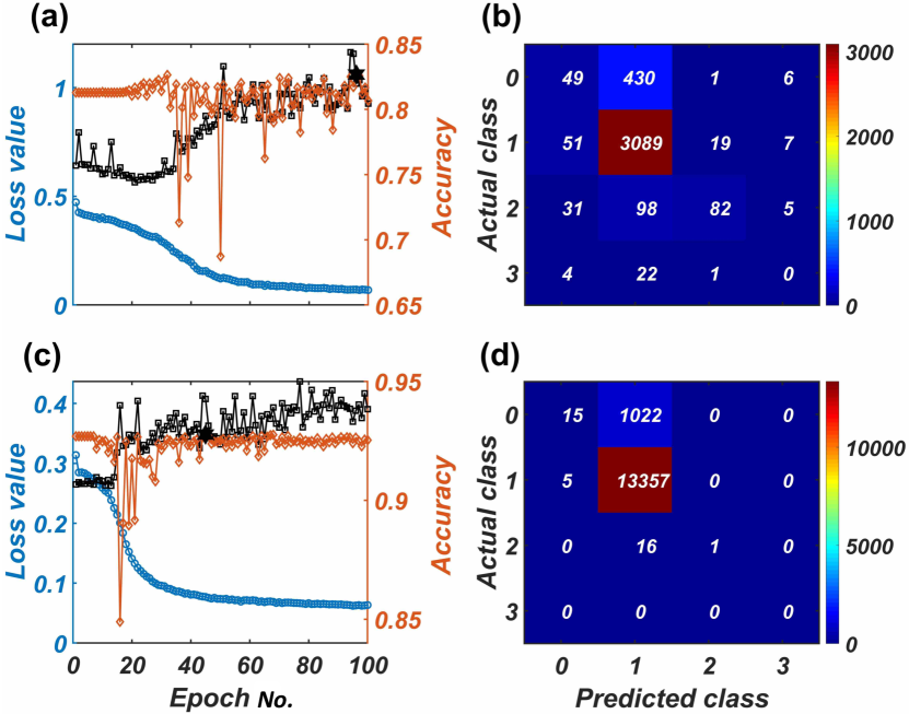
Figure 9: Results of DCNN based prediction of “where” an extreme wind speed will occur. (a) Losses (blue and black) and accuracy (brown) versus the epoch number for the restructured dataset, and (b) the confusion matrix corresponding to the best accuracy. (c,d) Results similar to those in (a,b) but for the forecast dataset. In all cases, the DCNN is ResNet-50, the labeling scheme is 2DLS, and the threshold in the wind speed for defining an extreme event is $30$m/s.

With the labeling scheme in Fig. 7(c), we can predict the location of the occurrence of an extreme wind speed after it has been predicted to occur within the prediction horizon. Representative results are shown in Fig. 9. As shown in Fig. 7, an image contains an extreme event if the 10-meter wind speed exceeds $30$ m/s. For two or more successive occurrences of extreme wind speed, we pick out the images corresponding to each event. This can cause duplication of some images in the training and testing datasets. The whole restructured and forecast datasets have $15579$ and $57664$ images, respectively, where the large difference is due to the occurrences of many consecutive extreme events. The restructured dataset has $1458$, $13482$, $594$, and $45$ wind speed images for classes ${\bf 0}$, ${\bf 1}$, ${\bf 2}$, and ${\bf 3}$, respectively, while the forecast datasets has $4114$, $53346$, $170$, and $34$ images for classes ${\bf 0}$, ${\bf 1}$, ${\bf 2}$, and ${\bf 3}$, respectively. The wind speed datasets are inevitably biased because there is an unbalanced distribution of extreme events in the North Atlantic ocean. For both the restructured and forecast datasets, we use the first $3/4$ as the training dataset and the remaining $1/4$ as the testing set. Figure 9(a) presents results of losses and accuracy for the restructured dataset, with the confusion matrix corresponding to the best accuracy is shown in Fig. 9(b). We see that the DCNN predictions are quite successful for classes $0$ and $2$, although most of the predicted events are for class $1$. The overall accuracy is about $82.7\%$. Figures 9(c) and 9(d) show the corresponding results but for the forecast dataset, where the overall accuracy is approximately $92.8\%$. The marked increase in the accuracy is due to the fact that more extreme events in the forecast dataset belong to class $1$ than those in the restructured dataset. The DCNN also predicts $15$ and $1$ correct images for classes ${\bf 0}$ and ${\bf 2}$, respectively. Taken together, our tests indicate that DCNN can be quite effective at predicting not only “when” extreme wind speed will occur within a predefined time interval but also “where” it will occur with reasonable accuracies. (In SI [55], we present the confusion matrices for a labeling scheme based on a $5\times 5$ spatial grid with $25$ classes, the “where” results for restructured and forecast datasets with no data overlap in the training and testing data, and the results of predicting “when” and “where” with the critical wind speed for defining an extreme event reduced to $26$ m/s.)

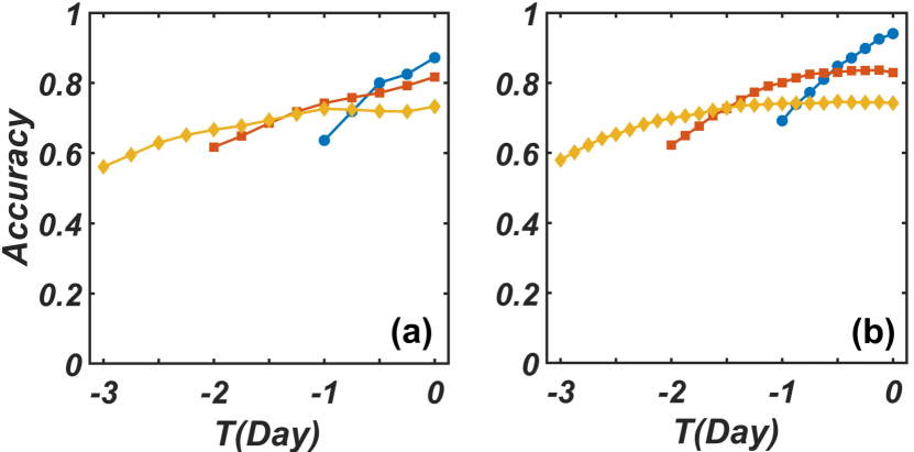
Figure 10: Accuracy of predicting when an extreme wind speed will occur at a series of time steps preceding the occurrence. In both panels, the abscissa denotes the time relative to the extreme event that occurs at time zero. For example, $-3$ means three days prior to the event. (a) For the restructured dataset, the prediction accuracy at each time step for 1DLS, 2DLS, and 3DLS (represented by the blue, brown, and yellow curves, respectively). (b) The same legends as in (a) but for the forecast dataset. The curves are generated with the threshold $FPR=0.15$ on the ROC curve. The wind speed threshold for extreme wind events is $30m/s$ and the DCNNs are of the ResNet-50 type. The parameters for the results in panels (a) and (b) are the same as those in Fig. 8(b) and Fig. 8(d), respectively.

To evaluate the performance of DCNN within the horizon of predicting “when” an extreme wind speed event would occur, we calculate the accuracy at each time step within the prediction horizon for both the restructured and forecast datasets, as shown in Figs. 10(a) and  10(b), respectively. It can be seen that the 1DLS labeling scheme has the best predictability for the state close to the extreme wind event, but the prediction accuracy decays quickly with the number of time steps prior to the extreme event. On the contrary, the labeling scheme 3DLS has the slowest decay in the prediction accuracy, because training the DCNN with more states can prolong the prediction horizon (in this case, to three days before the extreme event). However, the inclusion of more wind speed states decreases the importance of features of the states that are close to the extreme event, resulting in a low prediction accuracy for both the reconstructed and forecast datasets. Nevertheless, the prediction accuracy is still larger than the chance level 0.5. Figure 10 also reveals that the prediction accuracy is not one at time $T=0$, demonstrating that the DCNN does not simply rely on a threshold to predict the extreme wind speed event. Overall, the results in Fig. 10 indicate that the DCNN is capable of predicting “when” an extreme wind speed event will occur three days in advance reasonably accurately.

III Discussion

We have formulated the challenging problem of model-free prediction of extreme events in physical situations where a nonlinear dynamical process occurs in a two-dimensional spatial domain as an image recognition/classification problem in machine learning. While the spatiotemporal evolution of the physical field in such a domain is governed by 2D nonlinear PDEs, our framework requires no model and is completely data based. We have exploited DCNNs and demonstrated, using synthetic data from the CGLE and real empirical data of wind speed in the North Atlantic ocean, that when and where in the spatial domain extreme events would occur can be predicted with reasonable accuracies. Especially, we break the problem of spatiotemporal prediction into two parts: when and where an extreme event will occur. To address the issue of “when”, we set a desired prediction horizon in time, based on which spatiotemporal data in the form of consecutive snapshots (images) can be properly labeled. A DCNN successfully trained with a large number of labeled snapshots is then capable of predicting the occurrence of the extreme event within the predefined time horizon. Intuitively, there is a trade-off between the prediction horizon and accuracy: a longer horizon will inevitably reduce the accuracy, which has been demonstrated. The “where” problem can be solved after it has been predicted that an extreme event will occur within the prediction horizon, again through a proper labeling scheme based on a uniform division of the spatial domain. Another trade-off arises: the prediction accuracy will decrease with an increase in the resolution of the spatial domain leading to more classes of images to be predicted. We have tested two types of DCNN: LeNet-5 and ResNet-50, and found that the latter, a deeper neural networked system, performs relatively better.

We have studied two types of DCNN in this paper: LeNet-5 and ResNet-50, with the general problem setting of predicting to which class a state image belongs. This method can also be adopted to addressing image segmentation problems, where it is necessary to change the class in our labeling scheme to a representation mask. For example, class $0$ in predicting “where” an extreme event will occur by partitioning the spatial domain of interest to $4$ subdomains can be represented as a mask as $\begin{vmatrix}1&0\\ 0&0\end{vmatrix}$. DCNNs have been used widely in image segmentation, e.g., fully convolutional networks [56] and U-Net [57]. To exploit the DCNNs for image segmentation to predict “when” and “where” extreme events occur is an interesting topic of research.

For predicting extreme events in the CGLE, the accuracy achieved is quite remarkable and is generally markedly higher than predicting the extreme wind speed from empirical data, especially when predicting the location of its occurrence. The main culprit for the reduced accuracy with the real data lies in the inhomogeneous or biased occurrence of the extreme event in space, i.e., the probability of its occurrence is not uniform in the domain, in contrast to systems described by the CGLE where extreme events occur approximately uniformly in space. To develop a machine learning framework to predict extreme events in a 2D spatial domain with biased data is an issue that must be addressed in real applications, calling for further efforts in this field.

When applying the DCNN based prediction scheme to the wind speed datasets, in addition to the spatially inhomogeneous or biased occurrences of extreme wind speed event, the lack of sufficient extreme wind speed events is also a problem, as both can lead to the fast over-fitting of the DCNNs. With more available data together with fine-tuning the hyperparameters, the overfitting problem can be mitigated or even eliminated to enhance prediction performance.

The DCNN framework developed in this paper is anticipated to be applicable to real-world systems, for two reasons. First, DCNNs have enjoyed dramatic, unprecedented successes in many fields of science and engineering for complex tasks ranging from image recognition and classification to facial recognition to EI Niño/South Oscillation prediction. The basic idea underlying our prediction framework is that extreme events in 2D spatial domains can naturally be represented as “hot spots” in images, rendering the DCNN approach applicable. Second, DCNNs themselves are complex, high-dimensional nonlinear systems. Intuitively, insofar as properly DCNNs are able to overpower the target spatiotemporal dynamical systems in complexity, in principle the former will have the predictive power over the latter. In spite of the remarkable successes of DCNNs in solving all kinds of previously unsolvable problems, an open challenge is to understand its inner workings, giving birth to the field “Explainable Machine Learning.” At the present, the underlying mechanisms of DCNNs have not been understood, but this lack of understanding has not hindered the exploitation of DCNNs for solving sophisticated problems. In fact, designing suitable DCNNs to solve challenging problems, while postponing the formidable issue of gaining some basic understanding, has been a widely accepted practice in the scientific community. In addition to the type of spatiotemporal chaotic systems treated in this paper, there are other types of complex and chaotic systems exhibiting extreme events. Insofar as the available data from these systems can be organized as 2D images, our DCNN approach should generally be applicable. In particular, for any specific nonlinear system, the DCNNs need to be trained to learn the intrinsic rules governing the dynamical evolution of the images to make predictions.

It can happen that two extreme events occur within the same prediction horizon. We find that, when choosing the horizon to be $10$ time steps, such cases are rare (e.g., less than $4\%$ in the 2D CGLE system). If such a situation does arise, it will cause a small reduction in the prediction accuracy, due to the necessity to assign labels to images prior to the occurrence of the extreme events. In particular, to predict “when” an extreme event would occur, we label the images within the prediction horizon of an extreme event as one. If two extreme events occur during the same horizon, the images between these two extreme events are still labeled as one. However, to predict the spatial location of the extreme event (the “where” problem), the situation is slightly more complicated. Suppose two extreme events occurring within the same horizon belong to the same subdomain $\chi$. In this case, we duplicate the overlapping images between the two extreme events and directly label them and their replica as $\chi$. If two extreme events occurring in the same horizon belong to two different subdomains $\chi_{1}$ and $\chi_{2}$, we duplicate the overlapping images between these two extreme events and label them and their replica as $\chi_{1}$ and $\chi_{2}$. Inevitably, this labeling scheme will lead to errors as we assign some identical images to two distinct classes. However, the fraction of the overlapping images in the total dataset is negligibly small, leading to little reduction in the prediction accuracy.

In employing DCNNs to predict “when” and “where” extreme events occur in the CGLE with the demonstrated success, the temporal information about the dynamical evolution of the 2D state has in fact not been adequately exploited, as only static 2D images at a discrete set of time are used for training and prediction. For an input image, the DCNN machine only gives a time interval, with the present time as the starting point, during which an extreme event occurs. To develop a machine learning framework to take full advantage of the temporal information to achieve more reliable and accurate prediction is an outstanding problem.

Recently, there have been advances in exploiting reservoir computing machines, a class of recurrent neural networks articulated about two decades ago [58, 59], to predict the state evolution in spatiotemporal dynamical systems described by nonlinear PDEs [60, 61, 62, 63, 64, 65, 66, 67, 68, 69, 70] for about half dozen Lyapunov time. It thus seems possible to develop a framework based on reservoir computing to predict the precise time of occurrence of extreme events. We have conducted a pilot study of this idea with the CGLE, but the results obtained so far have not been promising. A plausible reason is that extreme events are relatively rare: starting from a random initial condition, it usually requires the system to evolve for a time much longer than half dozen Lyapunov times for an extreme event to occur. In fact, in spite of the deterministic nature of the CGLE system, the extreme events appear to occur randomly in both space and time. Since reservoir computing only involves one hidden layer and is designed to train a neural network to predict the state evolution of the target system, it may not be effective to deal with extreme events that are “quasi”-stochastic. In contrast, DCNNs, because of their sophisticated structure and vast complexity, are capable of predicting extreme events.

Another relevant issue concerns about the time scale of the target system and the determination of the prediction horizon. The parameter region in which the 2D CGLE system exhibits extreme events can have chaos in both space and time. The mean temporal period is an important characteristic time scale of the system. However, our DCNN based prediction framework should be applicable even to systems without a clearly defined time scale, because DCNNs are specially designed to recognize random spatial patterns. If the generation of an extreme event leads to the buildup of some distinct spatial pattern, then DCNN can be effective, regardless of whether the underlying dynamical system has a mean temporal period. The determination of the prediction horizon is also crucial. For systems with a natural cycle, it can be chosen as the prediction horizon. If a system does not have such a natural cycle, then the average correlation time or another physically meaningful time can be used. For example, for the North Atlantic wind speed dataset, the relevant time is one day or a few days. It is indeed desired to develop a more rigorous and theoretically justified criterion to determine the prediction horizon.

Appendix A Two-dimensional complex Ginzburg-Landau equation

Mathematically, the 2D CGLE is given by

$$\cfrac{\partial u}{\partial t}=\epsilon u+(\gamma+i\alpha)|u|^{2}u-(\mu+i\beta)\nabla^{2}u,$$ (1)

where $\epsilon$, $\gamma$, $\mu$, $\alpha$ and $\beta$ are dimensionless parameters. For $\epsilon=0$, $\gamma=0$, and $\mu=0$, the CGLE is reduced to the nonlinear Schrödinger equation (NLSE):

$$\cfrac{\partial u}{\partial t}=+i\alpha|u|^{2}u-i\beta\nabla^{2}u,$$ (2)

whose solutions diverge for $\alpha\beta>0$. In particular, for $\alpha\beta>1$, all solutions of the NLSE are unstable. In the parameter regime $(\gamma,\epsilon,\mu)\ll(\alpha,\beta)$, the regime in which the CGLE is close to the nonlinear Schrödinger equation, the system exhibits an intermittently bursting behavior in both space and time. From the solutions of the CGLE in the parameter regime near the NLSE limit, extreme or rare intense events in the form of spikes or bursts with “unusually” large amplitude can occur. The CGLE in this parameter regime thus represents a mathematical paradigm for studying extreme events in spatiotemporal dynamical systems.

In our study, we set $\epsilon=1$, $\gamma=1$, $\alpha=-30$, and $\beta=30$, so that the system generates extreme events that are random in both space and time. We solve the spatiotemporal evolution of the 2D state $u(x,y,t)$ on a square region of side length $l=10\pi$ in the $(x,y)$ plane with periodic boundary conditions using the pseudospectral and exponential-time differencing scheme [71]. Spatial discretization is accomplished by covering the domain with a uniform, $100\times 100$ grid. The integration time step is $dt=10^{-4}$. We perform sampling in the time domain on the numerical solution with $\Delta t=0.01$ to obtain a manageable set of 2D state images. For the parameter setting, the average temporal and spatial periods are approximately 0.09 and 5.09, respectively, corresponding to about $9$ time steps and the size of $16$ spatial cells in the resampled data set. Besides, the largest Lyapunov exponent of the system in this parameter setting is estimated to be $\lambda_{max}\approx 3.3$, so the Lyapunov time is $\Lambda_{t}=1/(\lambda_{max})\approx 0.3$. For the choice $\Delta t=0.01$, the prediction horizon is $10\Delta t=0.1$, which is within one Lyapunov time, rendering predictable the extreme event.

We also calculate the temporal correlation function $C_{st}(\tau)$ for the 2D CGLE system, which is defined as

$$C_{st}(\tau)=\langle\frac{\langle|u(x,y,t)u^{*}(x,y,t+\tau)|\rangle_{t}}{\langle|u(x,y,t)|^{2}\rangle_{t}}\rangle_{s},$$ (3)

where ^∗ denotes the complex conjugate, $\langle\cdot\rangle_{t}$ and $\langle\cdot\rangle_{s}$ are averages over time and space, respectively. We use $10^{4}$ sampling time steps to calculate the average over time. The result is shown in Fig. 1(f), where the decay time constant is about 10 time steps.

In our study, it took about nine hours for training $100$ epochs on ResNet-50 to predict when an extreme event would occur in the 2D CGLE on an NVIDIA GeForce RTX 3080 Laptop GPU. For the “where” problem, under the same setting, the time required for training was about two hours.

Appendix B Calculation of ROC curve

The detection of extreme events can be viewed as a binary classification problem. Let $x$ be the maximum field intensity in space, e.g., $|u|_{max}$ in the 2D CGLE or the maximum wind speed in North Atlantic ocean. For actual extreme events, $x$ follows a probability distribution with the density function $f_{1}(x)$. When, at a specific time instant, there is no extreme event in the space, then $x$ follows another probability distribution with the density function $f_{0}(x)$. By definition, on the $x$-axis, the center of $f_{1}(x)$ must be on the right side of the center of $f_{0}(x)$. To classify if a snapshot image possesses an extreme event, we set up a threshold value $X$, where if $x>X$ ($x<X$), then $x$ is regarded as belonging to $f_{1}(x)$ [$f_{0}(x)$]. With respect to a specific threshold value $X$, the true positive rate and false positive rate are given by

$$\mbox{TPR}(X) =\int^{\infty}_{X}f_{1}(x)dx\ \ \mbox{and}$$

$$\mbox{FPR}(X) =\int^{\infty}_{X}f_{0}(x)dx,$$

respectively. Let $[X_{1},X_{2}]$ be the range outside of which both $f_{0}(x)$ and $f_{1}(x)$ are zero. As $X$ is decreased from $X_{2}$ to $X_{1}$, both TPR and FPR continuously increase from zero to one.

In an actual situation, the probability density functions $f_{0}(x)$ and $f_{1}(x)$ are not known, so the TPR and FPR must be evaluated approximately by the relative frequencies. From our testing data consisting of a large number of images, the ground truth, i.e., whether an image contains an extreme event, is known. For a fixed threshold value $X$, the prediction of an extreme event from an image is either true or a false alarm. By sifting through all the images in the testing dataset, we can estimate the TPR and FPR values. Varying $X$ continuously in a proper range leads to systematically changing values of TPR and FPR, thereby generating the ROC curve. In our work, we use the MatLab function “perfcurve” to calculate the various ROC curves.

Appendix C Wind-speed datasets of North Atlantic ocean

We use the ERA-Interim datasets from European Centre for Medium-Range Weather Forecasts (ECMWF), downloaded from https://www.ecmwf.int. The details of the ERA-Interim datasets can be found in Ref. [72]. From the datasets, we extract 10-meter wind speed (wind speed at a height of 10 meters) data of the North Atlantic ocean, with $\mbox{latitude}\in[0^{\circ}N,70^{\circ}N]$ and $\mbox{longitude}\in[20^{\circ}W,90^{\circ}W]$. The dataset has a 40-year duration: from January 1, 1979 to December 31, 2018. There are two types of datasets: the restructured dataset with time interval of six hours and $58440$ wind-speed images in total, and the forecast dataset with time interval of three hours and $116880$ images. For both datasets, we set two wind-speed thresholds to define extreme events: $26$ m/s and $30$ m/s, corresponding to wind force scale $10$ and $11$, respectively, in the Beaufort scale [73].

References

- Albeverio et al. [2006] S. Albeverio, V. Jentsch, and H. Kantz, Extreme events in nature and society (Springer Science & Business Media, 2006).
- White and Fornberg [1998] B. S. White and B. Fornberg, On the chance of freak waves at sea, J. Fluid Mech. 355, 113 (1998).
- Solli et al. [2007] D. R. Solli, C. Ropers, P. Koonath, and B. Jalali, Optical rogue waves, Nature 450, 1054 (2007).
- Akhmediev et al. [2016] N. Akhmediev, B. Kibler, F. Baronio, M. Belić, W.-P. Zhong, Y.-Q. Zhang, W.-K. Chang, J. M. Soto-Crespo, P. Vouzas, and P. Grelu, Roadmap on optical rogue waves and extreme events, J. Opt. 18, 063001 (2016).
- Selmi et al. [2016] F. Selmi, S. Coulibaly, Z. Loghmari, I. Sagnes, G. Beaudoin, M. G. Clerc, and S. Barbay, Spatiotemporal chaos induces extreme events in an extended microcavity laser, Phys. Rev. Lett. 116, 013901 (2016).
- L’vov et al. [2001] V. S. L’vov, A. Pomyalov, and I. Procaccia, Outliers, extreme events, and multiscaling, Phys. Rev. E 63, 056118 (2001).
- Santhanam and Kantz [2005] M. S. Santhanam and H. Kantz, Long-range correlations and rare events in boundary layer wind fields, Physica A 345, 713 (2005).
- Altmann and Kantz [2005] E. G. Altmann and H. Kantz, Recurrence time analysis, long-term correlations, and extreme events, Phys. Rev. E 71, 056106 (2005).
- Nicolis et al. [2006] C. Nicolis, V. Balakrishnan, and G. Nicolis, Extreme events in deterministic dynamical systems, Phys. Rev. Lett. 97, 210602 (2006).
- Santhanam and Kantz [2008] M. Santhanam and H. Kantz, Return interval distribution of extreme events and long-term memory, Phys. Rev. E 78, 051113 (2008).
- Ansmann et al. [2013] G. Ansmann, R. Karnatak, K. Lehnertz, and U. Feudel, Extreme events in excitable systems and mechanisms of their generation, Phys. Rev. E 88, 052911 (2013).
- Bódai et al. [2013] T. Bódai, G. Károlyi, and T. Tél, Driving a conceptual model climate by different processes: Snapshot attractors and extreme events, Phys. Rev. E 87, 022822 (2013).
- Karnatak et al. [2014] R. Karnatak, G. Ansmann, U. Feudel, and K. Lehnertz, Route to extreme events in excitable systems, Phys. Rev. E 90, 022917 (2014).
- Mulhern et al. [2015] C. Mulhern, S. Bialonski, and H. Kantz, Extreme events due to localization of energy, Phys. Rev. E 91, 012918 (2015).
- Qi and Majda [2016] D. Qi and A. J. Majda, Predicting fat-tailed intermittent probability distributions in passive scalar turbulence with imperfect models through empirical information theory, Commun. Math. Sci. 14, 1687 (2016).
- Mohamad and Sapsis [2018] M. A. Mohamad and T. P. Sapsis, Sequential sampling strategy for extreme event statistics in nonlinear dynamical systems, Proc. Natl. Acad. Sci. (USA) 115, 11138 (2018).
- Bolles et al. [2019] C. T. Bolles, K. Speer, and M. N. J. Moore, Anomalous wave statistics induced by abrupt depth change, Phys. Rev. Fluids 4, 011801 (2019).
- Hallerberg et al. [2007] S. Hallerberg, E. G. Altmann, D. Holstein, and H. Kantz, Precursors of extreme increments, Phys. Rev. E 75, 016706 (2007).
- Donner and Barbosa [2008] R. V. Donner and S. M. Barbosa, Nonlinear time series analysis in the geosciences, Lecture Notes in Earth Sciences 112 (2008).
- Cavalcante et al. [2013] H. L. d. S. Cavalcante, M. Oriá, D. Sornette, E. Ott, and D. J. Gauthier, Predictability and suppression of extreme events in a chaotic system, Phys. Rev. Lett. 111, 198701 (2013).
- Bódai and Franzke [2017] T. Bódai and C. Franzke, Predictability of fat-tailed extremes, Phys. Rev. E 96, 032120 (2017).
- Nagy and Ott [2007] V. Nagy and E. Ott, Control of rare intense events in spatiotemporally chaotic systems, Phys. Rev. E 76, 066206 (2007).
- Du et al. [2008] L. Du, Q. Chen, Y.-C. Lai, and W. Xu, Observation-based control of rare intense events in the complex Ginzburg-Landau equation, Phys. Rev. E 78, 015201 (2008).
- Bialonski et al. [2015] S. Bialonski, G. Ansmann, and H. Kantz, Data-driven prediction and prevention of extreme events in a spatially extended excitable system, Phys. Rev. E 92, 042910 (2015).
- Lopatka [2019] A. Lopatka, Meteorologists predict better weather forecasting with AI, Phys. Today 72, 32 (2019).
- Hansen et al. [2000] J. Hansen, M. Sato, R. Ruedy, A. Lacis, and V. Oinas, Global warming in the twenty-first century: An alternative scenario, Proc. Natl. Acad. Sci. (USA) 97, 9875 (2000).
- Easterling et al. [2000] D. R. Easterling, J. Evans, P. Y. Groisman, T. R. Karl, K. E. Kunkel, and P. Ambenje, Observed variability and trends in extreme climate events: a brief review, Bull. Ame. Meteorol. Soc. 81, 417 (2000).
- Palmer and Räisänen [2002] T. Palmer and J. Räisänen, Quantifying the risk of extreme seasonal precipitation events in a changing climate, Nature 415, 512 (2002).
- Guardian [2012] T. Guardian, Scientists attribute extreme weather to man-made climate change, https://www.theguardian.com/environment/2012/jul/10/extreme-weather-manmade-climate-change (2012).
- for Environmental Information [2016] N. N. C. for Environmental Information, Billion-dollar weather and climate disasters: Summary stats, http://www.ncdc.noaa.gov/billions/summary-stats (2016).
- Stott [2016] P. Stott, How climate change affects extreme weather events, Science 352, 1517 (2016).
- Qi and Majda [2018] D. Qi and A. J. Majda, Predicting extreme events for passive scalar turbulence in two-layer baroclinic flows through reduced-order stochastic models, Commun. Math. Sci. 16, 17 (2018).
- Majda et al. [2019] A. J. Majda, M. N. J. Moore, and D. Qi, Statistical dynamical model to predict extreme events and anomalous features in shallow water waves with abrupt depth change, Proc. Natl. Acad. Sci. (USA) 116, 3982 (2019).
- LeCun et al. [2015] Y. LeCun, Y. Bengio, and G. Hinton, Deep learning, Nature 521, 436 (2015).
- Jordan and Mitchell [2015] M. I. Jordan and T. M. Mitchell, Machine learning: Trends, perspectives, and prospects, Science 349, 255 (2015).
- Goodfellow et al. [2016] I. Goodfellow, Y. Bengio, and A. Courville, Deep Learning (The MIT Press, Cambridge, Massachusetts, 2016).
- He et al. [2016] K. He, X. Zhang, S. Ren, and J. Sun, Deep residual learning for image recognition, in CVPR (2016) pp. 770–778.
- Krizhevsky et al. [2012] A. Krizhevsky, I. Sutskever, and G. E. Hinton, Imagenet classification with deep convolutional neural networks, in NeurIPS (2012) pp. 1097–1105.
- Hinton et al. [2012] G. Hinton, L. Deng, D. Yu, G. Dahl, A.-r. Mohamed, N. Jaitly, A. Senior, V. Vanhoucke, P. Nguyen, B. Kingsbury, et al., Deep neural networks for acoustic modeling in speech recognition, IEEE Signal Process. Mag. 29 (2012).
- Ma et al. [2015] J. Ma, R. P. Sheridan, A. Liaw, G. E. Dahl, and V. Svetnik, Deep neural nets as a method for quantitative structure–activity relationships, J. Chem. Inf. Model. 55, 263 (2015).
- Dang et al. [2020] W. Dang, Z. Gao, X. Sun, R. L. Li, Q. Cai, and C. Grebogi, Multilayer brain network combined with deep convolutional neural network for detecting major depressive disorder, Nonlin. Dyn. 102, 667 (2020).
- Silver et al. [2017] D. Silver, J. Schrittwieser, K. Simonyan, I. Antonoglou, A. Huang, A. Guez, T. Hubert, L. Baker, M. Lai, A. Bolton, et al., Mastering the game of go without human knowledge, Nature 550, 354 (2017).
- Reichstein et al. [2019] M. Reichstein, G. Camps-Valls, B. Stevens, M. Jung, J. Denzler, N. Carvalhais, et al., Deep learning and process understanding for data-driven earth system science, Nature 566, 195 (2019).
- Ham et al. [2019] Y.-G. Ham, J.-H. Kim, and J.-J. Luo, Deep learning for multi-year ENSO forecasts, Nature , 1 (2019).
- Guth and Sapsis [2019] S. Guth and T. P. Sapsis, Machine learning predictors of extreme events occurring in complex dynamical systems, Entropy 21, 925 (2019).
- Qi and Majda [2020] D. Qi and A. J. Majda, Using machine learning to predict extreme events in complex systems, Proc. Natl. Acad. Sci. (USA) 117, 52 (2020).
- LeCun et al. [1998] Y. LeCun, L. Bottou, Y. Bengio, P. Haffner, et al., Gradient-based learning applied to document recognition, Proc. IEEE 86, 2278 (1998).
- Ciresan et al. [2012] D. Ciresan, A. Giusti, L. M. Gambardella, and J. Schmidhuber, Deep neural networks segment neuronal membranes in electron microscopy images, in NeurIPS (2012) pp. 2843–2851.
- Farabet et al. [2012] C. Farabet, C. Couprie, L. Najman, and Y. LeCun, Learning hierarchical features for scene labeling, IEEE Trans. Pattern Anal. Mach. Intell. 35, 1915 (2012).
- Aranson and Kramer [2002] I. S. Aranson and L. Kramer, The world of the complex Ginzburg-Landau equation, Rev. Mod. Phys 74, 99 (2002).
- Cross and Hohenberg [1993] M. C. Cross and P. C. Hohenberg, Pattern formation outside of equilibrium, Rev. Mod. Phys. 65, 851 (1993).
- Kuramoto [1984] Y. Kuramoto, Chemical Oscillations, Waves and Turbulence (Springer, Berlin, 1984).
- Paszke et al. [2017] A. Paszke, S. Gross, S. Chintala, G. Chanan, E. Yang, Z. DeVito, Z. Lin, A. Desmaison, L. Antiga, and A. Lerer, Automatic differentiation in pytorch, in NIPS-W (2017).
- Paszke et al. [2019] A. Paszke, S. Gross, F. Massa, A. Lerer, J. Bradbury, G. Chanan, T. Killeen, Z. Lin, N. Gimelshein, L. Antiga, et al., Pytorch: An imperative style, high-performance deep learning library, in NIPS-W (2019) pp. 8024–8035.
- [55] See Supplemental Material at [URL will be inserted by publisher] for additional numerical results and specific details of the characterization method. However, the article can be fully understood without the Supplemental Material .
- Long et al. [2015] J. Long, E. Shelhamer, and T. Darrell, Fully convolutional networks for semantic segmentation, in CVPR (2015) pp. 3431–3440.
- Ronneberger et al. [2015] O. Ronneberger, P. Fischer, and T. Brox, U-net: Convolutional networks for biomedical image segmentation, in Med. Image. Comput. Comput. Assist. Interv. (Springer, 2015) pp. 234–241.
- Jaeger [2001] H. Jaeger, The “echo state” approach to analysing and training recurrent neural networks-with an erratum note, Bonn, Germany: German National Research Center for Information Technology GMD Technical Report 148, 13 (2001).
- Jaeger and Haas [2004] H. Jaeger and H. Haas, Harnessing nonlinearity: Predicting chaotic systems and saving energy in wireless communication, Science 304, 78 (2004).
- Haynes et al. [2015] N. D. Haynes, M. C. Soriano, D. P. Rosin, I. Fischer, and D. J. Gauthier, Reservoir computing with a single time-delay autonomous boolean node, Phys. Rev. E 91, 020801 (2015).
- Larger et al. [2017] L. Larger, A. Baylón-Fuentes, R. Martinenghi, V. S. Udaltsov, Y. K. Chembo, and M. Jacquot, High-speed photonic reservoir computing using a time-delay-based architecture: Million words per second classification, Phys. Rev. X 7, 011015 (2017).
- Pathak et al. [2018] J. Pathak, B. Hunt, M. Girvan, Z. Lu, and E. Ott, Model-free prediction of large spatiotemporally chaotic systems from data: A reservoir computing approach, Phys. Rev. Lett. 120, 024102 (2018).
- Carroll [2018] T. L. Carroll, Using reservoir computers to distinguish chaotic signals, Phys. Rev. E 98, 052209 (2018).
- Nakai and Saiki [2018] K. Nakai and Y. Saiki, Machine-learning inference of fluid variables from data using reservoir computing, Phys. Rev. E 98, 023111 (2018).
- Roland and Parlitz [2018] Z. S. Roland and U. Parlitz, Observing spatio-temporal dynamics of excitable media using reservoir computing, Chaos 28, 043118 (2018).
- Weng et al. [2019] T. Weng, H. Yang, C. Gu, J. Zhang, and M. Small, Synchronization of chaotic systems and their machine-learning models, Phys. Rev. E 99, 042203 (2019).
- Jiang and Lai [2019] J. Jiang and Y.-C. Lai, Model-free prediction of spatiotemporal dynamical systems with recurrent neural networks: Role of network spectral radius, Phys. Rev. Res. 1, 033056 (2019).
- Vlachas et al. [2020] P. R. Vlachas, J. Pathak, B. R. Hunt, T. P. Sapsis, M. Girvan, E. Ott, and P. Koumoutsakos, Backpropagation algorithms and reservoir computing in recurrent neural networks for the forecasting of complex spatiotemporal dynamics, Neural Net. 126, 191 (2020).
- Fan et al. [2020] H. Fan, J. Jiang, C. Zhang, X. Wang, and Y.-C. Lai, Long-term prediction of chaotic systems with machine learning, Phys. Rev. Research 2, 012080 (2020).
- Kong et al. [2021] L.-W. Kong, H.-W. Fan, C. Grebogi, and Y.-C. Lai, Machine learning prediction of critical transition and system collapse, Phys. Rev. Research 3, 013090 (2021).
- Cox and Matthews [2002] S. M. Cox and P. C. Matthews, Exponential time differencing for stiff systems, J. Comput. Phys. 176, 430 (2002).
- Dee et al. [2011] D. P. Dee, S. Uppala, A. Simmons, P. Berrisford, P. Poli, S. Kobayashi, U. Andrae, M. Balmaseda, G. Balsamo, d. P. Bauer, et al., The era-interim reanalysis: Configuration and performance of the data assimilation system, Q. J. Roy. Meteor. Soc. 137, 553 (2011).
- Singleton [2008] F. Singleton, The beaufort scale of winds–its relevance, and its use by sailors, Weather 63, 37 (2008).