Exponential Approach to the Hydrodynamic Attractor
in Yang-Mills Kinetic Theory

Abstract

We use principal component analysis to study the hydrodynamic attractor in Yang-Mills kinetic theory undergoing the Bjorken expansion with Color Glass Condensate initial conditions. The late time hydrodynamic attractor is characterized by a single principal component determining the overall energy scale. How it is reached is governed by the disappearance of single subleading principal component characterizing deviations of the pressure anisotropy, the screening mass and the scattering rate. We find that for wide range of couplings the approach to the hydrodynamic attractor at late times is well described by an exponential. Its decay rate dependence on the coupling turns out to translate into a simple dependence on the shear viscosity to entropy density ratio.

I Introduction

Ultrarelativistic heavy-ion collisions at RHIC and LHC produce a collective state of matter comprised of the fundamental quark and gluon constituents of strong interactions. Describing ab initio formation and evolution of this quark-gluon plasma (QGP) presents an important theoretical problem. Since a first principles description directly using the theory of strong force, quantum chromodynamics (QCD), remains an outstanding challenge, the standard model of the space-time evolution of heavy-ion collisions is based on effective descriptions of QCD Heinz (2013). The initial non-equilibrium dynamics after the collision has been addressed in a variety of different microscopic models Schlichting and Teaney (2019); Berges et al. (2021). Eventually, on a time scale of $\sim 1\,\rm{fm}/c$, the QGP can be well described by relativistic hydrodynamics. This is to some extent surprising, as the system can feature large spatial and temporal gradients and remains significantly out of equilibrium for a much longer period of time, as indicated e.g. by large values of the pressure anisotropy.

Due to these concerns the applicability of relativistic hydrodynamics in high-energy collisions of heavy and light nuclei has repeatedly been questioned Romatschke (2017a), and different proposals have been put forward to extend the applicability of hydrodynamics to earlier times and more anisotropic systems Florkowski et al. (2018). One proposal to potentially extend the validity of hydrodynamics goes by the name of hydrodynamic attractors Heller and Spalinski (2015), which represent emergent constitutive relations away from equilibrium. Over the course of the last few years, the emergence of such hydrodynamics attractors has been firmly established in a variety of effectively 0+1 dimensional microscopic models which feature a rather high degree of symmetry Romatschke (2018); Strickland et al. (2018); Strickland (2018); Jaiswal et al. (2019); Blaizot and Yan (2020); Almaalol et al. (2020); Heller et al. (2020); Du and Schlichting (2021a), and different theoretical Romatschke (2017b); Behtash et al. (2018); Denicol and Noronha (2018, 2020); Kurkela et al. (2020); Blaizot and Yan (2021); Behtash et al. (2021); Du et al. (2021); Chattopadhyay et al. (2022) and phenomenological aspects of the emergence of hydrodynamic attractors Kurkela et al. (2019a); Giacalone et al. (2019); Jankowski et al. (2021); Coquet et al. (2021) have been explored. See Soloviev (2021) for a recent review.

Despite efforts in this direction Romatschke (2017b); Ambrus et al. (2021), the generalization of the concept of hydrodynamic attractors to higher dimensional systems represents an outstanding challenge. With this as a motivation, it was recently pointed out that the hydrodynamic attractor can be viewed as a dimensionality reduction in a space of natural observables associated with nuclear collision problems Heller et al. (2020). From this perspective, the number of relevant degrees of freedom required to describe the evolution of a system is effectively lowered due to a rapid memory loss of initial conditions. Viewing thermalization in this way enables to approach the study of thermalization in a data-driven way and borrow methods from data science.

In the present work we adopt the approach of Heller et al. (2020) to study the evolution of a 0+1D Bjorken flow in an effective kinetic theory (EKT) of pure glue QCD Kurkela et al. (2019a); Giacalone et al. (2019) with highly anisotropic color glass condensate Gelis et al. (2010); Iancu and Venugopalan (2003) initial conditions. Building on the methodology developed in Heller et al. (2020), we use principal component analysis (PCA) to study the dimensionality reduction for a set of observables that describe the thermalization process at weak coupling. The mechanism behind the information loss can come from the expansion at early time or interactions at late times Blaizot and Yan (2018); Kurkela et al. (2020). We also look more closely at the late time behaviour to gain information on transient non-hydrodynamic contributions to the pressure anisotropy, and compare our results in pure glue QCD kinetic theory to previous studies in conformal Relaxation Time Approximation (RTA) Heller et al. (2018a); Heller and Svensson (2018).

The paper is organized in the following way: In Sec. II, we introduce our model of the initial state, along with the effective kinetic theory of pure glue QCD describing the non-equilibrium dynamics of the QGP. Subsequently, in Sec. III, we perform a PCA of the evolution for different initial conditions to study information loss and dimensionality reduction over the course of the thermalization process of the pre-equilibrium QGP. Sec. IV is devoted to a more detailed study of the evolution towards equilibrium, focusing on the exponential decay of variance of the pressure anisotropy in the QGP. We conclude this paper in Sec. V with a short summary of our most important findings and an outlook on potential future works.

II Setup

We use the Color Glass Condensate (CGC) effective theory of high-energy QCD Gelis et al. (2010); Iancu and Venugopalan (2003), to evaluate the phase-space distributions of gluons produced in the collision. Due to physical differences and uncertainties in modeling the initial state, this gives rise to a multi-dimensional parameter space of early time phase-space distributions of gluons. They serve as initial conditions for EKT, which we subsequently utilize to evolve expanding nuclear matter into the hydrodynamic phase.

II.1 Color Glass Condensate initial conditions

We will compute the initial spectrum of gluons based on the $k_{T}$-factorization formula  Blaizot et al. (2010); Lappi and Schlichting (2018)

$$\frac{dN_{g}}{d^{2}\mathbf{b}d^{2}\mathbf{P}dy}=\frac{g^{2}N_{c}}{4\pi^{5}\mathbf{P}^{2}(N_{c}^{2}-1)}$$ (1)

$$\int\frac{d^{2}\mathbf{k}}{(2\pi)^{2}}~{}\Phi_{A}(\mathbf{b}+\frac{\mathbf{b}_{0}}{2},\mathbf{k})\Phi_{B}(\mathbf{b}-\frac{\mathbf{b}_{0}}{2},\mathbf{P}-\mathbf{k})\;.$$

where $\frac{dN_{g}}{d^{2}\mathbf{b}d^{2}\mathbf{P}dy}$ describes the transverse momentum $(\mathbf{P})$ spectrum of gluons produced per unit rapidity $(y)$ and transverse area $(\mathbf{b})$. By $N_{c}=3$ we denote the number of colors, $g$ is the Yang-Mills coupling, $\mathbf{b}_{0}$ denotes the impact parameter of the nucleus-nucleus collision and $\phi_{A/B}(\mathbf{b},\mathbf{k})$ is the un-integrated gluon distribution from each nucleus (A or B). We employ a particularly simple parametrization of the nuclear gluon distributions, due to Golec-Biernat and Wusthoff (GBW) Golec-Biernat and Wusthoff (1998), for which

$$\Phi_{A,B}(\mathbf{b},\mathbf{k})=4\pi^{2}\frac{(N_{c}^{2}-1)}{g^{2}N_{c}}\frac{\mathbf{k}^{2}}{Q_{\rm A,B}^{2}(\mathbf{b})}\exp\left(\frac{-\mathbf{k}^{2}}{Q_{A,B}^{2}(\mathbf{b})}\right)$$ (2)

where $Q_{A,B}^{2}=Q_{s}^{2}(\mathbf{b})$ denotes the (adjoint) saturation scale Albacete and Marquet (2014) for nucleus.

Based on Eqns. (1) and (2), the initial gluon spectrum in the GBW model can then be expressed analytically as

$$\frac{dN_{g}}{d^{2}\mathbf{b}d^{2}\mathbf{P}dy}=\frac{(N_{c}^{2}-1)}{g^{2}N_{c}\pi^{2}\mathbf{P}^{2}}$$ (3)

$$\frac{x^{2}e^{-\mathbf{P}^{2}/Q^{2}}}{Q^{2}}\left(\frac{\mathbf{P}^{4}x^{2}+\mathbf{P}^{2}(1-x^{2})^{2}Q^{2}+2x^{2}Q^{4}}{(1+x^{2})^{4}}\right)$$

where $Q\equiv\sqrt{Q_{A}^{2}+Q_{B}^{2}}$ and $x\equiv\max\left(\frac{Q_{B}}{Q_{A}},\frac{Q_{A}}{Q_{B}}\right)$ denote the root mean square average and the ratio of the saturation scales. Since the saturation scales $Q_{A/B}^{2}$ are generically proportional to local density of nuclear matter, we can anticipate that for different collision geometries the ratio $x=Q_{A}/Q_{B}$ will vary, and we will consider variations $1\leq x\leq 6$ in the following.

Since the transverse spectrum in Eq. (3) features a $\propto 1/\mathbf{P}^{2}$ infrared behavior, soft observables, such as screening mass $m_{D}$ and scattering rate $g^{2}T^{*}$ in Eq. (14), are infrared divergent. However, this divergence can be regulated by non-linear effects, going beyond the factorization formula, see e.g. the discussion in  Blaizot et al. (2010). Within our study, we will simply model this by introducing an additional infrared regulator, by virtue of the replacement $\frac{1}{\mathbf{P}^{2}}\to\frac{\mathbf{P}^{2}}{(\mathbf{P}^{2}+m^{2})^{2}}$ in the first factor of Eq. (3), which ensures that $m_{D}$ and $g^{2}T^{*}$ in Eq. (14) remain finite, while the initial energy density is not affected by the regulator as long as $\text{max}(Q_{A}^{2},Q_{B}^{2})\gg m^{2}$. Since corrections to the factorization formula become important for $\mathbf{P}\lesssim\min(Q_{A},Q_{B})$, in the following we choose the infrared regulator as $\mu\equiv\frac{m}{Q}=\frac{\min(Q_{A},Q_{B})}{2Q}$. We further note that due to the particular simplicity of the GBW model, the initial spectrum in Eq. (3) exhibits and exponential decay at high momentum $\mathbf{P}\gtrsim Q$, whereas a more realistic parametrization should give rise to a $Q^{4}/\mathbf{P}^{4}$ power-law tail Dumitru and McLerran (2002). However, since the energy density of the system is dominated by momenta $\mathbf{P}\sim Q$, we believe that the model is adequate to study the thermalization of the bulk QGP, while neglecting the impact of high-energy degrees of freedom.

Based on the transverse momentum spectrum, the initial phase-space distribution $f(x,p)$ can then be obtained as Greif et al. (2017)

$$f_{g}(\tau_{0},\mathbf{b},\mathbf{P},y-\eta)=\frac{(2\pi)^{3}}{2(N_{c}^{2}-1)}\frac{\delta(y-\eta)}{|\mathbf{P}|\tau_{0}}\frac{dN_{g}}{d^{2}\mathbf{b}d^{2}\mathbf{P}dy}$$ (4)

where $\eta$ denotes the space-time rapidity and we employ these as initial conditions for the subsequent kinetic description at an initial proper time $\tau_{0}=1/Q$, where a quasi-particle description first becomes applicable Schlichting and Teaney (2019); Berges et al. (2021). While in the high-energy boost-invariant limit, the initial distribution is proportional to $\delta(y-\eta)$, any interactions will immediately broaden the longitudinal momentum distribution and we therefore consider a smearing form of the delta function

$$\delta(y-\eta)\to\frac{1}{\sqrt{2\pi}\sigma}\exp\left(-\frac{(y-\eta)^{2}}{2\sigma^{2}}\right).$$ (5)

in the initial conditions. We treat the width of longitudinal rapidity distribution $\sigma$ as the second free parameter in the initial conditions and consider variations in the range $0.05<\sigma<0.50$ in the following.

Starting from the phase-space distribution, the energy-momentum tensor $T^{\mu\nu}$ is defined as a its second moment

$$T^{\mu\nu}=\nu_{g}\int\frac{d^{3}p}{(2\pi)^{3}}\frac{p^{\mu}p^{\nu}}{p}f_{g}(\tau,\mathbf{b},\mathbf{P},y-\eta)\;.$$ (6)

where $\nu_{g}=2(N_{c}^{2}-1)$ denotes the degeneracy factor for gluons. Specifically, one may evaluate the energy density $\epsilon$, the transverse and the longitudinal pressure $P_{T/L}$ in Milne coordinates as

$$\epsilon = T^{\tau\tau}~{}~{}=\int\frac{d^{2}\mathbf{P}}{(2\pi)^{2}}\frac{dp_{\|}}{(2\pi)}~{}p~{}\nu_{g}f_{g}(\tau,\mathbf{b},\mathbf{P},p_{\|}),$$ (7a)

$$P_{T} = T^{ii}/2=\int\frac{d^{2}\mathbf{P}}{(2\pi)^{2}}\frac{dp_{\|}}{(2\pi)}\frac{|\mathbf{P}|^{2}}{2p}\nu_{g}f_{g}(\tau,\mathbf{b},\mathbf{P},p_{\|}),\quad$$ (7b)

$$P_{L} = \tau^{2}T^{\zeta\zeta}=\int\frac{d^{2}\mathbf{P}}{(2\pi)^{2}}\frac{dp_{\|}}{(2\pi)}\frac{p_{\|}^{2}}{p}\nu_{g}f_{g}(\tau,\mathbf{b},\mathbf{P},p_{\|}),\quad$$ (7c)

where we have re-expressed the phase-space distribution $f_{g}$ in terms of the momentum variables $p=p^{\tau}=\sqrt{\mathbf{P}^{2}+p_{\|}^{2}}$ and $p_{\|}=\tau p^{\eta}=|\mathbf{P}|\mathrm{sinh}(y-\eta)$. They denote the total and the longitudinal momentum in the co-moving frame.

When considering variations of the parameters $x$ and $\sigma$, we adjust the value of the average saturation scale $Q$, to keep the initial transverse pressure per unit rapidity $g^{2}\tau_{0}P_{T}$ (which is independent of the coupling $g$) constant in physical units. Hence the parameter space of the initial conditions is two dimensional and spanned by the ratio of the nuclear saturation scales $x$ and the longitudinal smearing width $\sigma$.

II.2 Effective kinetic theory of pure glue QCD

We model the evolution of excited nuclear matter using kinetic description. We follow previous works Kurkela and Zhu (2015); Kurkela et al. (2019b); Almaalol et al. (2020) and treat the system as longitudinally boost-invariant and locally homogeneous in the transverse plane. The dynamics reduces to a (0+1)-dimensional problem and is governed by an effective kinetic for pure glue QCD Arnold et al. (2003a)

$$\left(\frac{\partial}{\partial\tau}-\frac{p_{\|}}{\tau}\frac{\partial}{\partial p_{\|}}\right)f_{g}(\tau,\mathbf{P},p_{\|})$$ (8)

$$=-C^{{2\leftrightarrow 2}}_{g}[f_{g}](\tau,\mathbf{P},p_{\|})-C^{{1\leftrightarrow 2}}_{g}[f_{g}](\tau,\mathbf{P},p_{\|})\;,$$

where $C^{{2\leftrightarrow 2}}_{g}[f]$ denotes the leading order elastic collision integral for gluons and $C^{{1\leftrightarrow 2}}_{g}[f]$ is the inelastic collision integral that describes emission/absorption of gluon radiation

$$C^{{2\leftrightarrow 2}}_{g}[f](p) = \frac{1}{2\nu_{g}2E_{p}}\int\frac{d^{3}p_{2}}{(2\pi)^{3}2E_{p_{2}}}\frac{d^{3}p_{3}}{(2\pi)^{3}2E_{p_{3}}}\frac{d^{3}p_{4}}{(2\pi)^{3}2E_{p_{4}}}(2\pi)^{4}\delta^{(4)}(p+p_{2}-p_{3}-p_{4})|\mathcal{M}_{gg\rightarrow gg}(p,p_{2}|p_{3},p_{4})|^{2}$$ (9a)

$$\times \left(f(p)f(p_{2})(1+f(p_{3}))f(1+f(p_{4}))-f(p_{3})f(k_{4})(1+f(p))f(1+f(p_{2}))\right),$$

$$C^{{1\leftrightarrow 2}}_{g}[f](p) = \frac{1}{2}\int_{0}^{1}dz\left\{\frac{d\Gamma_{gg}^{g}}{dz}(p,z)\left[f(p)(1+f(zp))(1+f(\bar{z}p)))-f(zp)f(\bar{z}p)(1+f(p))\right]\right.$$ (9b)

$$- \left.\frac{1}{z^{3}}\frac{d\Gamma_{gg}^{g}}{dz}\left(\frac{p}{z},z\right)\left[f\left(\frac{p}{z}\right)(1+f(p))\left(1+f\left(\frac{\bar{z}}{z}p\right)\right)-f(p)f\left(\frac{\bar{z}}{z}p\right)\left(1+f\left(\frac{p}{z}\right)\right)\right]\right\}.$$

We note that the matrix element $|\mathcal{M}_{gg\rightarrow gg}(p,p_{2}|p_{3},p_{4})|^{2}$ for elastic scattering is self-consistently screened following the prescription of Kurkela and Mazeliauskas (2019), and that the effective inelastic rates $\frac{d\Gamma_{gg}^{g}}{dz}(p,z)$ account for the Landau-Pomeranchuk-Migdal effect Landau and Pomeranchuk (1953a, b); Migdal (1955) via an effective vertex resummation Arnold et al. (2003a). Details of the algorithms and numerical implementations can be found in Du and Schlichting (2021b). Early initialization requires a fine discretization of the momentum space variables for the EKT simulations, and if not stated otherwise we employ $N_{p}=1024$ and $N_{\cos(\theta)}=512$ to discretize $p$ and $\cos{\theta}=\frac{p_{\|}}{p}$ in the range between $p_{\rm min}/(g^{2}\tau_{0}P_{T})^{1/3}=0.01$ and $p_{\rm max}/(g^{2}\tau_{0}P_{T})^{1/3}=20$.

Finally, note that in pure glue QCD kinetic theory the interaction strength $g$ and the number of colors $N_{c}$ enter the Boltzmann together as the ’t Hooft coupling $\lambda$ Abraao York et al. (2014)

$$\lambda\equiv g^{2}N_{c}.$$ (10)

Therefore, in the following we will express the interaction strength in terms of $\lambda$.

III Early time dynamics, attractors & dimensionality reduction

III.1 Hydrodynamization & Emergence of attractors

One prominent indicator of transition to hydrodynamics is the longitudinal pressure over what would be the equilibrium pressure ratio $P_{L}/(\epsilon/3)$ or any of its closely related variants. We present it in Fig. 1 as a function of the universal time scale Heller et al. (2012); Keegan et al. (2016); Heller et al. (2018b); Du and Schlichting (2021a)

$$\tilde{w}=\frac{\tau(\epsilon+P)}{4\pi\upeta}.$$ (11)

where $\upeta$ is the shear viscosity and $P=\epsilon/3$ is the thermodynamic pressure for a conformal system. It can be thought of as measuring the physical proper time in units of an effective equilibrium relaxation time

$$\tau_{R}=\frac{4\pi\upeta}{\epsilon+P}\equiv\frac{1}{T}\frac{\upeta}{s}/\frac{1}{4\pi},$$ (12)

where $T$ is an effective temperature of non-equilibrium system determined by $\epsilon=\nu_{g}\frac{\pi^{2}T^{4}}{30}$ and $s$ is the entropy density. While the overall scaling with $T$ follows on dimensional grounds for a conformal system, the normalization factor of $1/4\pi$ is conventional and inspired by the strong coupling result $\upeta/s=1/4\pi$ of Policastro et al. (2001); Kovtun et al. (2005).

Different colored curves in Fig. 1 show to the results obtained for different ratios of the saturation scales $x$ and different longitudinal smearing width $\sigma$. Different dash styles correspond to the evolution for three different coupling strengths $\lambda=5,10,20$, for which the relevant viscosities $\upeta/s\sim\mathcal{O}(1)$ as summarized in Tab. 1 in the Appendix.

Starting from the initial conditions, one observes a significant variation of $P_{L}/(\epsilon/3)$, where small smearing parameters $\sigma$ feature a highly anisotropic initial distribution, with almost vanishing longitudinal pressure. Since in all cases the initial time $\tau_{0}=1/Q$ is kept fixed, the curves for different simulation parameters $x,\sigma,\lambda$ start at different values of $\tilde{w}$; in this way larger saturation scale ratios $x$ also tends to provide relevantly more anisotropic initial distribution.

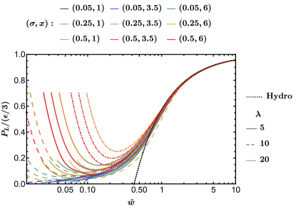
Figure 1: Evolution of the ratio of the longitudinal pressure to what would the equilibrium pressure $P_{L}/(\epsilon/3)$ as a function of the conformal scaling variable $\tilde{w}$ in Eq. (11). Different curves show results from pure glue QCD kinetic theory simulations for different initial conditions $(\sigma,x)$ at three different coupling strength $\lambda$=5,10,20.

During the initial stages the evolution is dominated by the longitudinal expansion of the system Blaizot and Yan (2018); Kurkela et al. (2020), such that the ratio of $P_{L}/(\epsilon/3)$ undergoes a quick memory loss and at intermediate times approaches a small value irrespective of the initial conditions. Eventually, on a time scale $\tilde{w}\simeq 1$, all the different curves merge towards the hydrodynamic limit, which to first order in gradients can be universally expressed as Heller et al. (2018b)

$$\left(\frac{P_{L}}{\epsilon/3}\right)_{\rm hydro}=1-\frac{16}{3}\frac{\upeta}{(\epsilon+P)\tau}=1-\frac{4}{3\pi\tilde{w}}\;.$$ (13)

While the emergence of a pressure attractor at $0.1<\tilde{w}<1$ clearly indicates an early reduction of the variance due to the initial free-streaming expansion dynamics, it is equally important to point out that the full convergence to a common attractor only occurs at later times $\tilde{w}>1$, when the system relaxes towards hydrodynamics.

III.2 Principal component analysis

Next, in order to better understand the emergence and properties of the attractor in pure glue QCD kinetic theory, we will scrutinize the evolution further by including additional observables, which go beyond probing the bulk anisotropy of the system. Beyond the anisotropic pressure $P_{L}$ and $P_{T}$ in Eqns. (15), we will study the screening mass $m_{D}^{2}$ and the collision rate $g^{2}T_{*}$

$$m_{D}^{2} = \frac{4g^{2}}{d_{A}}\int\frac{d^{3}p}{(2\pi)^{3}}\frac{\nu_{g}C_{A}f_{g}(\vec{p})}{2p}\overset{(eq)}{=}\frac{g^{2}N_{c}T_{\rm eq}^{2}}{3}$$ (14)

$$T_{*} = \frac{g^{2}}{d_{A}m_{D}^{2}}\int\frac{d^{3}p}{(2\pi)^{3}}\bigg{\{}\nu_{g}C_{A}f_{g}(\vec{p})(1+f_{g}(\vec{p}))\bigg{\}}\overset{(eq)}{=}T_{\rm eq}.$$

Since $m_{D}^{2}$ and $g^{2}T^{*}$ govern the strength of elastic and inelastic interactions in pure glue QCD kinetic theory, they present the most natural quantities to include in a weak coupling analysis.

Since all of of the above quantities $P_{L},P_{T},m_{D}^{2},T_{*}$ are dimensionful, it is natural to consider dimensionless ratios along with one single quantity that is sensitive to the overall energy scale. Specifically, for our analysis, we choose to consider $P_{L}/(\epsilon/3)$ and normalize $m_{D}^{2},T_{*}$ by the transverse pressure $P_{T}$. This gives us the following dimensionless quantities

$$\bar{P}_{L} \equiv\frac{P_{L}}{\epsilon/3},$$ (15a)

$$\bar{m}_{D}^{2} \equiv\frac{m_{D}^{2}}{(90P_{T}/\pi^{2}\nu_{g})^{1/2}g^{2}N_{c}/3},$$ (15b)

$$\bar{T}_{*} \equiv\frac{T_{*}}{(90P_{T}/\pi^{2}\nu_{g})^{1/4}}.$$ (15c)

All of them by construction approach unity in thermal equilibrium. While initially, the transverse pressure $$P_{T}$$ is kept constant for different initial conditions, differences in the kinetic evolution gives rise to variations of the overall energy scale, which we monitor in terms of the dimensionless quantity

$$\bar{P}_{T} \equiv\frac{\tau^{4/3}P_{T}}{1/3(2P_{T0}\tau_{0})^{8/9}(\frac{\pi^{2}}{30}\nu_{g})^{1/9}(4\pi\frac{\upeta}{s})^{4/9}C_{\infty}}.$$ (15d)

where we employ $C_{\infty}=0.98$ Giacalone et al. (2019). By following the arguments of Giacalone et al. (2019); Du and Schlichting (2021a), the denominator in Eq. (15d) provides an estimate for the late time asymptotic value of $\tau^{4/3}P_{T}$, such that for typical initial conditions this quantity can again be expected to be close to unity at late times.

We can directly verify these expectations in Fig. 2, where we present the evolution of the observables $\bar{P}_{T},\bar{P}_{L},\bar{m}_{D}^{2},\bar{T}_{*}$ as a function of the universal time scale $\tilde{w}$ for a variety of different initial conditions at three different coupling strengths $\lambda=5,10,20$. While the self-normalized quantities $\bar{P}_{L},\bar{m}_{D}^{2},\bar{T}_{*}$ all converge to a common attractor behavior at late times, the overall energy scale $\bar{P}_{T}$ develops a $\sim 15\%$ variation over the course of the non-equilibirum evolution of the system.

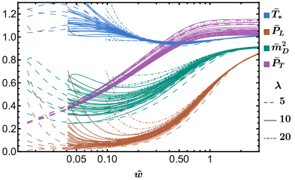
Figure 2: Evolution of the observables $\bar{P}_{T},\bar{P}_{L},\bar{m}_{D}^{2},\bar{T}_{*}$ as a function of the universal time scale $\tilde{w}$ for a variety of different initial conditions at three different coupling strengths $\lambda=5,10,20$. The observable $\bar{P}_{T}$ has been chosen to contain the information on the overall energy scale and features the only sizable variation at late times. Conversely, all other observables are insensitive to the overall energy scale and show an attractor behaviour.

With the set of observables in Eq. (15), we can further perform a PCA to extract the most significant contributions in the emergence of the attractor phenomenon, namely the principal components of the attractor. For this purpose, rather than studying these quantities separately, we can also consider these quantities as parametrizing a four dimensional space. Each solution is represented as a vector

$$\mathbf{X}(\tilde{w})=\begin{pmatrix}\bar{T}_{*}(\tilde{w})&\bar{P}_{L}(\tilde{w})&\bar{m}_{D}^{2}(\tilde{w})&\bar{P}_{T}(\tilde{w})\end{pmatrix}$$ (16)

evolving in time. Evidently, to perform a meaningful comparison of the different directions in $\mathbf{X}(\tilde{w})$ space, the units and overall scales of the different components of $\mathbf{X}(\tilde{w})$ must be comparable, which is precisely the reason that the observables have been normalized as in Eq. (15).

From this point of view, thermalization is achieved through dimensionality reduction. With sufficient variation of the initial phase-space distribution function, the set of initial conditions $\{\mathbf{X}_{0}\}$ collectively spans some volume in the four dimensional space. However, since the initial conditions used here only depend on two parameters, we only expect to span (at most) a two dimensional subspace. Over the course of the thermalization process, the dimensionless variables $\bar{P}_{L},\bar{m}_{D}^{2},\bar{T}_{*}$ all approach unity, and only $\bar{P}_{T}$ which is sensitive to the overall energy scale should have a significant variation at late times, implying that ultimately the solutions will span a one dimensional subspace.

PCA is a simple method to study this process of dimensionality reduction. Given a set of points $\{\mathbf{X}\}$, the PCA calculates the eigenvectors and eigenvalues of the covariance matrix

$$\mathbf{C}_{mn}=\operatorname{Cov}(\mathbf{X}_{m},\mathbf{X}_{n}).$$ (17)

to produce a set of orthonormal vectors such that the first vector points along the direction of the largest variance of the data set, and the subleading vectors are similarly optimized in the space orthogonal to the leading vector. Each vector is associated with an explained variance, quantified by the variance of the set of points in its direction. The number of non-negligible explained variances gives a measure of the dimensionality of the region occupied by the states of interest at a given value of time variable.

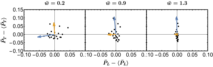
Figure 3: Snapshots of the evolution of an ensemble of different initial conditions in the $\bar{P}_{L}$,$\bar{P}_{T}$ plane at three different times $\tilde{w}=0.2,0.9,1.3$ for $\lambda=10$. Each point corresponds to the evolution for a particular initial condition; blue and orange arrows indicate the first and second principle components. While initially the points are scattered in the two-dimensional plane, they collapse onto a one dimensional subspace at late times. The length of the vectors is set to three times the square root the of the explained variance for better visibility.

We illustrate this behavior in Fig. 3, where we show the distribution of values in the $\bar{P}_{L}$,$\bar{P}_{T}$ plane at three different times $\tilde{w}=0.2,0.9,1.3$ of the evolution. Each point in Fig. 3 corresponds to the evolution for a particular initial condition, while the blue and orange arrows indicate the first and second principle components. While at early times $(\tilde{w}=0.2)$ the different initial conditions cover a two-dimensional subspace, with the largest variations in the $\bar{P}_{L}$ direction, the effective reduction of the dimensionality of the distribution is clearly visible, as at late times $\tilde{w}=1.3$ all points converge towards a one dimensional manifold oriented along the $\bar{P}_{T}$ direction.

By applying PCA to the set of solutions at each point in the universal time $\tilde{w}$, we can study the dimensionality of the dataset through the explained variances, and identify which directions in the space of observables that show the greatest variance. Our results are compactly summarized in Figs. 4 and 5, where we show the evolution of the explained variances along with the evolution of the composition of two dominant principle component vectors. One clearly observes from Fig. 4, that at late times, there is indeed only a single dominant component, which is associated with an approximately constant explained variance. Beyond the leading principal component, the explained variance of the second most relevant component decays approximately exponentially at times $\tilde{w}\gtrsim 0.5$.

Figure 4: Explained variances for the observables in Fig. 2. The colors distinguish between different principal components, ordered by the explained variance. Starting from a complicated behavior at early times, the only relevant contributions at late times are associated with a single dominant component that remains approximately constant and a second component which is approximately exponentially decaying. Separate contributions of the different observables to the these two principal components are shown in Fig. 5.

The decomposition of the first and second principal components are shown in Fig. 5. The abrupt shift in behaviour at $\tilde{w}\approx 0.5$ is correlated with the crossing of explained variances in Fig. 4, and should be thought of as the two vectors switching identity. At late times the first component is dominated by $\bar{P}_{T}$, which was chosen to be sensitive to the energy scale of the state. The second component is dominated by $\bar{P}_{L}$ and $\bar{m}_{D}^{2}$.

While Fig. 2 already shows that the observables $\bar{m}_{D}^{2},\bar{T}_{*}$ also features a similar attractor behaviour as the well-known $\bar{P}_{L}$, it does not tell us whether these attractors are actually the same. In contrast, the principal component analysis in Figs. 4 and 5 reveals that the evolution of the different observables is highly correlated and can be captured with a single principal component.

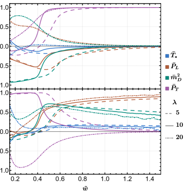
Figure 5: Decomposition of the leading (top) and first subleading (bottom) principal component vectors. By design, the leading vector is dominated by $\bar{P}_{T}$, which carries information about the overall energy scale. The second principal component corresponds to an exponentially decaying transient, and characterizes the variation in the other observables. Since no other principal component is sizable, we learn that the observables $\bar{m}_{D}^{2},\bar{T}_{*},\bar{P}_{L}$ are highly correlated and governed by the same attractor.

IV Evolution towards equilibrium

So far we have statistically analyzed the emergence of hydrodynamics attractors starting from CGC initial conditions at very early times $\tilde{w}\ll 1$. While in this case the dynamics is initially dominated by the longitudinal expansion, we performed additional simulations that focus on the late time approach to hydrodynamic behavior to further analyze the memory loss and convergence towards hydrodynamic behavior in pure glue QCD kinetic theory. By initializing the system according to a Romatschke-Strickland type distribution Romatschke and Strickland (2003),

$$f_{g}(\tau_{0},\mathbf{P},p_{\|})=\frac{c(\xi_{0})}{e^{\frac{\sqrt{\mathbf{P}^{2}+\xi_{0}^{2}p_{\|}^{2}}}{T_{0}}}-1}$$ (18)

for different initial anisotropies $\xi_{0}=1.25,2.5,5,10$ at initial time $\tilde{w}_{0}=0.1,0.3$ and $\xi_{0}=1.1,1.2,1.3$ at initial time $\tilde{w}_{0}=1,3,10$, we are then able to analyze the effective memory loss at late times for a large range of couplings $\lambda=0.1-20$. We note that in all cases, the normalization factor

$$c(\xi_{0})=\frac{2}{1/\xi_{0}^{2}+\text{arctan}(\sqrt{\xi_{0}^{2}-1})/\sqrt{\xi_{0}^{2}-1}}$$ (19)

is chosen such that the initial energy density $\epsilon(\tilde{w}_{0})=\frac{\pi^{2}}{30}\nu_{g}T_{0}^{4}$ remains the same irrespective of the initial anisotropy $\xi_{0}$; while in order to initialize the simulations at the same $\tilde{w}_{0}$, the initial proper time is adjusted as $\tau_{0}=\frac{4\pi\upeta/s}{T_{0}}\tilde{w}_{0}$ in Eq. (18) for the respective coupling strength. For completeness, our numerical implementation employs the following discretization: $N_{p}=64$ and $N_{\cos(\theta)}=64$ with $p_{\rm min}/T_{0}=0.01$ and $p_{\rm max}/T_{0}=8$.

IV.1 Exponential approach to hydrodynamics at late times

In order to investigate direct approach to viscous hydrodynamics at late times, we will focus on the evolution of $P_{L}/(\epsilon/3)$ in $\tilde{w}$. As we discussed in Sec. III.2, this quantity has a significant contribution to the leading principal component characterising deviations from the attractor, and exhibits a universal late time hydrodynamic behavior determined by Eq. (13).

The evolution of the $P_{L}/(\epsilon/3)$ for the initial conditions (18) is depicted in Fig. 6. Different colored curves correspond to the results for different coupling strength $\lambda=0.1-20$, while curves of the same color correspond to different initial conditions $\xi_{0}$ at different initialization times $\tilde{w}_{0}$. Irrespective of the coupling strength, one observes that very quickly after the initialization, different initial conditions appear to converge towards a common attractor curve. By careful inspection, one notes that for varying coupling strength slight differences in the attractors persist at intermediate times $\tilde{w}\lesssim 3$, before eventually all curves converge towards the same (by construction) hydrodynamic late time behavior (13). Note that contributions from the terms second and higher order in derivatives are expected to exhibit residual coupling dependence, which might at least partially explain the slight differences between attractors at earlier times.

In order to further characterize the approach towards an attractor, we compute the variances of $P_{L}/(\epsilon/3)$ for the different initial conditions $\xi_{0}$ at each value of the initialization time $\tilde{w}_{0}$ and coupling strength $\lambda$. Before we discuss our results in pure glue QCD kinetic theory, shown in the middle panel of Fig. 6, it proves insightful to recall the behavior previously observed in different microscopic models of early-time dynamics of the QGP.

Starting with Heller and Spalinski (2015) (see also Başar and Dunne (2015); Aniceto and Spaliński (2016) for a more complete discussion), it was understood that in a class of models employing the Müller-Israel-Stewart (MIS) approach to embed hydrodynamics in a framework compatible with relativistic causality Muller (1967); Israel (1976); Israel and Stewart (1979), the late time behavior of $P_{L}/(\epsilon/3)$ can be elevated into a transseries Aniceto et al. (2019a) of the form

$$\frac{P_{L}}{\epsilon/3}=\sum_{n=0}^{\infty}\frac{b_{n}}{\tilde{w}^{n}}+\sum_{j}e^{-\Omega_{j}\tilde{w}}\tilde{w}^{\beta}_{j}\sum_{n=0}^{\infty}\frac{b_{j,n}}{\tilde{w}^{n}}.$$ (20)

Without dwelling into details of this formal expression, the key aspect for us are exponentially suppressed in times effects with decay rates associated with $\Omega_{j}$. In MIS different $\Omega_{j}$ are just integer multiples (due to nonlinear effects) of a single relaxation scale present in this class of theories. The same structure was verified to appear in RTA kinetic theory Heller et al. (2018a); Heller and Svensson (2018); Heller et al. (2021) and in holography Heller et al. (2013); Casalderrey-Solana et al. (2018); Aniceto et al. (2019b); Heller et al. (2021).

Most importantly, the contributions $\Omega_{i}$ describe the decay of transient non-hydrodynamic contributions to the pressure anisotropy, which in the aforementioned examples can be related to the analytic structure of retarded correlation functions of the energy-momentum tensor in equilibrium Kovtun and Starinets (2005); Florkowski et al. (2018). In the conformal RTA kinetic theory the shear viscosity and the relaxation time are related by

$$\tau_{\text{r}}(\tau)=\frac{5\upeta}{sT(\tau)}.$$ (21)

Following Janik and Peschanski (2006), the relaxation time determines the decay rate of non-hydrodynamic contributions in the boost-invariant background as

$$-\int\frac{d\tau}{\tau_{\text{r}}(\tau)}=-\int\frac{T(\tau)d\tau}{5\upeta/s}\approx-\frac{3}{2}\frac{T(\tau)\tau}{5\upeta/s}=-\frac{6}{5}\pi\tilde{w},$$ (22)

where we have used the fact that $T(\tau)$ scales as $\tau^{-1/3}$ at sufficiently late times in Bjorken flow and dropped subleading contributions at late time. While Eq. (22) provides the rate of decay of non-hydrodynamic contributions in each individual realization, the variance measures the square of these contributions and thus decays twice as fast.

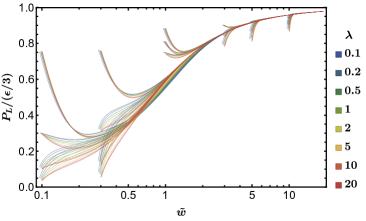
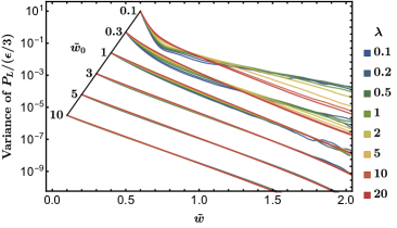
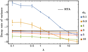
Figure 6: (top) Evolution of the pressure to what would be the equilibrium pressure ratio $p_{L}/(\epsilon/3)$. (middle) Evolution of variance of $P_{L}/(\epsilon/3)$. The exponential decay is associated to decay of non-hydrodynamic contributions to $P_{L}/(\epsilon/3)$. (bottom) Exponential decay rates of the variance extracted from the middle figure. Different points are obtained by varying the extraction range and the curve is formed from the mean result.

While the structure of non-hydrodynamic excitations in QCD kinetic theory is generally expected to be rather complicated Kurkela and Wiedemann (2019); Moore (2018), it is nevertheless interesting to investigate to what extent a simple parametrization of the type in Eq. (20) can describe the convergence towards an attractor.

To this end, inspection of the evolution of the variances in the middle plot in Fig. 6 shows a clear exponential decay of the variance for most values of $\lambda$ and $\tilde{w}_{0}$. Clear deviations from an exponential decay are only seen for data initialized at very early times, particularly for small coupling, where subleading contributions to the pressure anisotropy can be expected to be more important.

We extract the effective decay rate $\Omega_{\rm eff}$ of the variance for each choice of $\lambda$ and $\tilde{w}_{0}$ by a linear fit in a variety of windows. Extracted values of the decay rate are presented in the bottom plot of Fig. 6, along with the mean value of those fits and for comparison we also show the decay rate $\frac{12}{5}\pi$ in conformal RTA kinetic theory.

While not perfectly exponential, the data initialized at early times have a smaller effective decay rate at smaller couplings. For the data initialized at late times, which show a clear exponential decay, the decay rate is approximately independent of the coupling strength $\lambda$ (with variations within 5% as the coupling varies by over two orders of magnitude) and turns out to be rather close to the value in RTA.

While our finding suggests that, just like in RTA, the decay rate in QCD kinetic theory appears to be closely connected to the value of viscosity, we certainly do not have a good explanation of this behavior. We note however, that similar observations were made also at the level of second order transport coefficients York and Moore (2009). In particular, this implies that the contribution at $\tilde{w}^{-2}$ in Eq. (13) exhibits very weak residual dependence on the coupling $\lambda$.

V Summary & Outlook

We have studied the transition to hydrodynamics of Yang-Mills kinetic theory undergoing Bjorken expansion. For initial conditions inspired by the CGC effective theory, we analyzed the subsequent evolution of a natural set of four observables given by Eq. (15) using PCA. Such an analysis may be sensitive to the precise initial conditions used, which is why we studied realistic initial conditions from the CGC effective theory.

Our studies showed that at late times there is a single dominant principal component that describes the variation of the overall energy scale $\bar{P}_{T}$. Furthermore, the late time evolution of $\bar{P}_{L}$, $\bar{m}_{D}^{2}$ and $\bar{T}^{*}$ is highly correlated and can be captured by a second subleading principal component. While at this point it remains a logical possibility that this correlation is an artifact of the considered initial conditions, this could be further explored within a higher dimensional parameter space.

The second principal component represents a transient contribution, which we studied in more detail by considering $\bar{P}_{L}$ using other initial conditions initialized at different times. A clear exponential decay can be seen at late times by comparing different profiles of $\bar{P}_{L}$, signaling the presence of an exponential approach to the hydrodynamic attractor at late times.

Quite surprisingly, for the whole range of the couplings considered, i.e. for $\lambda$ between 0.1 and 20, the decay rate is close to the value predicted by the conformal RTA kinetic theory. What this means in practical terms is that the effective decay rate is simply expressible in terms of the shear viscosity-to-entropy density ratio, see Eq. (21).

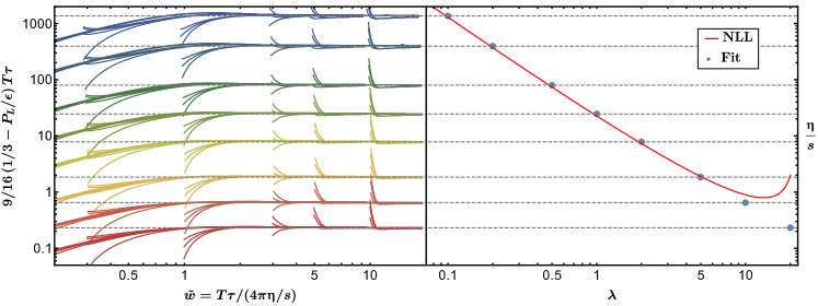
Figure 7: (left) Extraction of the shear viscosity to entropy density ratio $\upeta/s$ from the late time hydrodynamic behavior of Yang-Mills kinetic theory simulations. (right) Extracted values of $\upeta/s$ as a function of $\lambda=g^{2}N_{c}$. See Table 1 for numerical values.

It is an interesting question to ask if the similarities between the EKT and conformal RTA go beyond this crude characteristic. To this end, an in-depth analysis of the RTA kinetic theory in Heller and Svensson (2018) reveals that the exponentially decaying contribution there is not a single excitation, but actually a sum of infinitely many contributions whose occupation numbers are initial condition dependent. While they all are characterized by the same exponential decay rate, their subleading behaviour is distinct yet impossible to disentangle over the short time scales probed in the present project. This indicates that in reality the exponential decay we are reporting here is likely to be understood as an effective description (appropriate for the conformal Bjorken flow with no transverse dynamics) of an underlying more complicated structure.

Beyond further explorations of the surprising similarity in the highly symmetric Bjorken flow, it would also be interesting to compare the evolution of the energy-momentum tensor in a variety of other settings. While first steps in this direction have been reported in Kamata et al. (2020); Kurkela et al. (2019b) for linearized perturbations around Bjorken flow and in  Kurkela et al. (2019c); Ambrus et al. (2022, 2021) for systems undergoing both longitudinal and transverse expansion, a particularly clean probe concerns the evolution of energy-momentum (or metric) perturbations in equilibrium. While for conformal RTA kinetic theory the corresponding retarded correlators of the energy-momentum tensor were calculated analytically in Romatschke (2016), a dedicated study in QCD kinetic theory would certainly shed further light on the structure and importance of non-hydrodynamic excitations. One can view the results of Kurkela and Wiedemann (2019) obtained in RTA kinetic theory with momentum-dependent relaxation time (see, however, Rocha et al. (2021) for a subtlety in this model that emerged after Kurkela and Wiedemann (2019) was completed) as a first step in this direction.

*

Appendix A Extraction of $\upeta/s$

Below we explain our procedure for the extraction of the shear-viscosity to entropy density ratio $\upeta/s$ from the kinetic theory simulations. Starting point of the extraction, is the universal hydrodynamic late time behavior, where the ratio of longitudinal pressure to energy density behaves as

$$\frac{P_{L}}{\epsilon}=\frac{1}{3}-\frac{16}{9}\frac{\upeta/s}{\tau T}+\ldots.$$ (23)

By inverting Eq. (23) for $\upeta/s$, we can use the ratio $9/16(1/3-P_{L}/\epsilon)T\tau$ to extract the ratio of shear viscosity to entropy density $\upeta/s$ from the asymptotic behavior of each numerical solution, and in subsequent analysis we use the mean value for each $\lambda$. We illustrate this extraction in the left panel of Fig. 7, while the right panel of Fig. 7 shows the extracted values in comparison to NLL parametrization of $\upeta/s$ in Arnold et al. (2003b). We note that for small couplings $\lambda$, the extracted values of $\upeta/s$ are in excellent agreement with the NLL parametrization, while for larger values of $\lambda$ the NLL parametrization breaks down, and as discussed in Kurkela and Mazeliauskas (2019) the transport coefficients also become more sensitive to the precise implementation of the screening of the elastic matrix elements. We also provide the extracted values in Table 1.

$\lambda$	0.1	0.2	0.5	1	2	5	10	20
$\upeta/s$	1361	394.9	79.69	24.55	7.845	1.848	0.6472	0.2313

Table 1: Numerically extracted viscosity, averaged over different solutions. These values were used in the subsequent analysis.

References

- Heinz (2013) U. W. Heinz, Towards the Little Bang Standard Model, J. Phys. Conf. Ser. 455, 012044 (2013), arXiv:1304.3634 [nucl-th] .
- Schlichting and Teaney (2019) S. Schlichting and D. Teaney, The first fm/c of heavy-ion collisions, Annual Review of Nuclear and Particle Science 69, 447–476 (2019).
- Berges et al. (2021) J. Berges, M. P. Heller, A. Mazeliauskas, and R. Venugopalan, QCD thermalization: Ab initio approaches and interdisciplinary connections, Rev. Mod. Phys. 93, 035003 (2021), arXiv:2005.12299 [hep-th] .
- Romatschke (2017a) P. Romatschke, Do nuclear collisions create a locally equilibrated quark–gluon plasma?, Eur. Phys. J. C 77, 21 (2017a), arXiv:1609.02820 [nucl-th] .
- Florkowski et al. (2018) W. Florkowski, M. P. Heller, and M. Spalinski, New theories of relativistic hydrodynamics in the LHC era, Rept. Prog. Phys. 81, 046001 (2018), arXiv:1707.02282 [hep-ph] .
- Heller and Spalinski (2015) M. P. Heller and M. Spalinski, Hydrodynamics Beyond the Gradient Expansion: Resurgence and Resummation, Phys. Rev. Lett. 115, 072501 (2015), arXiv:1503.07514 [hep-th] .
- Romatschke (2018) P. Romatschke, Relativistic Fluid Dynamics Far From Local Equilibrium, Phys. Rev. Lett. 120, 012301 (2018), arXiv:1704.08699 [hep-th] .
- Strickland et al. (2018) M. Strickland, J. Noronha, and G. Denicol, Anisotropic nonequilibrium hydrodynamic attractor, Phys. Rev. D 97, 036020 (2018), arXiv:1709.06644 [nucl-th] .
- Strickland (2018) M. Strickland, The non-equilibrium attractor for kinetic theory in relaxation time approximation, JHEP 12, 128, arXiv:1809.01200 [nucl-th] .
- Jaiswal et al. (2019) S. Jaiswal, C. Chattopadhyay, A. Jaiswal, S. Pal, and U. Heinz, Exact solutions and attractors of higher-order viscous fluid dynamics for Bjorken flow, Phys. Rev. C 100, 034901 (2019), arXiv:1907.07965 [nucl-th] .
- Blaizot and Yan (2020) J.-P. Blaizot and L. Yan, Emergence of hydrodynamical behavior in expanding ultra-relativistic plasmas, Annals Phys. 412, 167993 (2020), arXiv:1904.08677 [nucl-th] .
- Almaalol et al. (2020) D. Almaalol, A. Kurkela, and M. Strickland, Nonequilibrium Attractor in High-Temperature QCD Plasmas, Phys. Rev. Lett. 125, 122302 (2020), arXiv:2004.05195 [hep-ph] .
- Heller et al. (2020) M. P. Heller, R. Jefferson, M. Spaliński, and V. Svensson, Hydrodynamic Attractors in Phase Space, Phys. Rev. Lett. 125, 132301 (2020), arXiv:2003.07368 [hep-th] .
- Du and Schlichting (2021a) X. Du and S. Schlichting, Equilibration of the Quark-Gluon Plasma at Finite Net-Baryon Density in QCD Kinetic Theory, Phys. Rev. Lett. 127, 122301 (2021a), arXiv:2012.09068 [hep-ph] .
- Romatschke (2017b) P. Romatschke, Relativistic Hydrodynamic Attractors with Broken Symmetries: Non-Conformal and Non-Homogeneous, JHEP 12, 079, arXiv:1710.03234 [hep-th] .
- Behtash et al. (2018) A. Behtash, C. N. Cruz-Camacho, and M. Martinez, Far-from-equilibrium attractors and nonlinear dynamical systems approach to the Gubser flow, Phys. Rev. D 97, 044041 (2018), arXiv:1711.01745 [hep-th] .
- Denicol and Noronha (2018) G. S. Denicol and J. Noronha, Analytical attractor and the divergence of the slow-roll expansion in relativistic hydrodynamics, Phys. Rev. D 97, 056021 (2018), arXiv:1711.01657 [nucl-th] .
- Denicol and Noronha (2020) G. S. Denicol and J. Noronha, Exact hydrodynamic attractor of an ultrarelativistic gas of hard spheres, Phys. Rev. Lett. 124, 152301 (2020), arXiv:1908.09957 [nucl-th] .
- Kurkela et al. (2020) A. Kurkela, W. van der Schee, U. A. Wiedemann, and B. Wu, Early- and Late-Time Behavior of Attractors in Heavy-Ion Collisions, Phys. Rev. Lett. 124, 102301 (2020), arXiv:1907.08101 [hep-ph] .
- Blaizot and Yan (2021) J.-P. Blaizot and L. Yan, Analytical attractor for Bjorken flows, Phys. Lett. B 820, 136478 (2021), arXiv:2006.08815 [nucl-th] .
- Behtash et al. (2021) A. Behtash, S. Kamata, M. Martinez, T. Schäfer, and V. Skokov, Transasymptotics and hydrodynamization of the Fokker-Planck equation for gluons, Phys. Rev. D 103, 056010 (2021), arXiv:2011.08235 [hep-ph] .
- Du et al. (2021) Z. Du, X.-G. Huang, and H. Taya, Hydrodynamic attractor in a Hubble expansion, Phys. Rev. D 104, 056022 (2021), arXiv:2104.12534 [nucl-th] .
- Chattopadhyay et al. (2022) C. Chattopadhyay, S. Jaiswal, L. Du, U. Heinz, and S. Pal, Non-conformal attractor in boost-invariant plasmas, Phys. Lett. B 824, 136820 (2022), arXiv:2107.05500 [nucl-th] .
- Kurkela et al. (2019a) A. Kurkela, A. Mazeliauskas, J.-F. Paquet, S. Schlichting, and D. Teaney, Matching the Nonequilibrium Initial Stage of Heavy Ion Collisions to Hydrodynamics with QCD Kinetic Theory, Phys. Rev. Lett. 122, 122302 (2019a), arXiv:1805.01604 [hep-ph] .
- Giacalone et al. (2019) G. Giacalone, A. Mazeliauskas, and S. Schlichting, Hydrodynamic attractors, initial state energy and particle production in relativistic nuclear collisions, Phys. Rev. Lett. 123, 262301 (2019), arXiv:1908.02866 [hep-ph] .
- Jankowski et al. (2021) J. Jankowski, S. Kamata, M. Martinez, and M. Spaliński, Constraining the initial stages of ultrarelativistic nuclear collisions, Phys. Rev. D 104, 074012 (2021), arXiv:2012.02184 [nucl-th] .
- Coquet et al. (2021) M. Coquet, X. Du, J.-Y. Ollitrault, S. Schlichting, and M. Winn, Intermediate mass dileptons as pre-equilibrium probes in heavy ion collisions, Phys. Lett. B 821, 136626 (2021), arXiv:2104.07622 [nucl-th] .
- Soloviev (2021) A. Soloviev, Hydrodynamic attractors in heavy ion collisions: a review, (2021), arXiv:2109.15081 [hep-th] .
- Ambrus et al. (2021) V. E. Ambrus, S. Busuioc, J. A. Fotakis, K. Gallmeister, and C. Greiner, Bjorken flow attractors with transverse dynamics, Phys. Rev. D 104, 094022 (2021), arXiv:2102.11785 [nucl-th] .
- Gelis et al. (2010) F. Gelis, E. Iancu, J. Jalilian-Marian, and R. Venugopalan, The Color Glass Condensate, Ann. Rev. Nucl. Part. Sci. 60, 463 (2010), arXiv:1002.0333 [hep-ph] .
- Iancu and Venugopalan (2003) E. Iancu and R. Venugopalan, The Color glass condensate and high-energy scattering in QCD, in Quark-gluon plasma 4, edited by R. C. Hwa and X.-N. Wang (2003) pp. 249–3363, arXiv:hep-ph/0303204 .
- Blaizot and Yan (2018) J.-P. Blaizot and L. Yan, Fluid dynamics of out of equilibrium boost invariant plasmas, Phys. Lett. B 780, 283 (2018), arXiv:1712.03856 [nucl-th] .
- Heller et al. (2018a) M. P. Heller, A. Kurkela, M. Spaliński, and V. Svensson, Hydrodynamization in kinetic theory: Transient modes and the gradient expansion, Physical Review D 97, 091503 (2018a).
- Heller and Svensson (2018) M. P. Heller and V. Svensson, How does relativistic kinetic theory remember about initial conditions?, Physical Review D 98, 054016 (2018).
- Blaizot et al. (2010) J. P. Blaizot, T. Lappi, and Y. Mehtar-Tani, On the gluon spectrum in the glasma, Nucl. Phys. A 846, 63 (2010), arXiv:1005.0955 [hep-ph] .
- Lappi and Schlichting (2018) T. Lappi and S. Schlichting, Linearly polarized gluons and axial charge fluctuations in the Glasma, Phys. Rev. D 97, 034034 (2018), arXiv:1708.08625 [hep-ph] .
- Golec-Biernat and Wusthoff (1998) K. J. Golec-Biernat and M. Wusthoff, Saturation effects in deep inelastic scattering at low Q**2 and its implications on diffraction, Phys. Rev. D 59, 014017 (1998), arXiv:hep-ph/9807513 .
- Albacete and Marquet (2014) J. L. Albacete and C. Marquet, Gluon saturation and initial conditions for relativistic heavy ion collisions, Prog. Part. Nucl. Phys. 76, 1 (2014), arXiv:1401.4866 [hep-ph] .
- Dumitru and McLerran (2002) A. Dumitru and L. D. McLerran, How protons shatter colored glass, Nucl. Phys. A 700, 492 (2002), arXiv:hep-ph/0105268 .
- Greif et al. (2017) M. Greif, C. Greiner, B. Schenke, S. Schlichting, and Z. Xu, Importance of initial and final state effects for azimuthal correlations in p+Pb collisions, Phys. Rev. D 96, 091504 (2017), arXiv:1708.02076 [hep-ph] .
- Kurkela and Zhu (2015) A. Kurkela and Y. Zhu, Isotropization and hydrodynamization in weakly coupled heavy-ion collisions, Phys. Rev. Lett. 115, 182301 (2015), arXiv:1506.06647 [hep-ph] .
- Kurkela et al. (2019b) A. Kurkela, A. Mazeliauskas, J.-F. Paquet, S. Schlichting, and D. Teaney, Effective kinetic description of event-by-event pre-equilibrium dynamics in high-energy heavy-ion collisions, Phys. Rev. C 99, 034910 (2019b), arXiv:1805.00961 [hep-ph] .
- Arnold et al. (2003a) P. B. Arnold, G. D. Moore, and L. G. Yaffe, Effective kinetic theory for high temperature gauge theories, JHEP 01, 030, arXiv:hep-ph/0209353 .
- Kurkela and Mazeliauskas (2019) A. Kurkela and A. Mazeliauskas, Chemical equilibration in weakly coupled QCD, Phys. Rev. D 99, 054018 (2019), arXiv:1811.03068 [hep-ph] .
- Landau and Pomeranchuk (1953a) L. Landau and I. Pomeranchuk, Electron cascade process at very high-energies, Dokl. Akad. Nauk Ser. Fiz. 92, 735 (1953a).
- Landau and Pomeranchuk (1953b) L. Landau and I. Pomeranchuk, Limits of applicability of the theory of bremsstrahlung electrons and pair production at high-energies, Dokl. Akad. Nauk Ser. Fiz. 92, 535 (1953b).
- Migdal (1955) A. B. Migdal, Quantum kinetic equation for multiple scattering, Dokl. Akad. Nauk Ser. Fiz. 105, 77 (1955).
- Du and Schlichting (2021b) X. Du and S. Schlichting, Equilibration of weakly coupled QCD plasmas, Phys. Rev. D 104, 054011 (2021b), arXiv:2012.09079 [hep-ph] .
- Abraao York et al. (2014) M. C. Abraao York, A. Kurkela, E. Lu, and G. D. Moore, UV cascade in classical Yang-Mills theory via kinetic theory, Phys. Rev. D 89, 074036 (2014), arXiv:1401.3751 [hep-ph] .
- Heller et al. (2012) M. P. Heller, R. A. Janik, and P. Witaszczyk, The characteristics of thermalization of boost-invariant plasma from holography, Phys. Rev. Lett. 108, 201602 (2012), arXiv:1103.3452 [hep-th] .
- Keegan et al. (2016) L. Keegan, A. Kurkela, P. Romatschke, W. van der Schee, and Y. Zhu, Weak and strong coupling equilibration in nonabelian gauge theories, JHEP 04, 031, arXiv:1512.05347 [hep-th] .
- Heller et al. (2018b) M. P. Heller, A. Kurkela, M. Spaliński, and V. Svensson, Hydrodynamization in kinetic theory: Transient modes and the gradient expansion, Phys. Rev. D 97, 091503 (2018b), arXiv:1609.04803 [nucl-th] .
- Policastro et al. (2001) G. Policastro, D. T. Son, and A. O. Starinets, The Shear viscosity of strongly coupled N=4 supersymmetric Yang-Mills plasma, Phys. Rev. Lett. 87, 081601 (2001), arXiv:hep-th/0104066 .
- Kovtun et al. (2005) P. Kovtun, D. T. Son, and A. O. Starinets, Viscosity in strongly interacting quantum field theories from black hole physics, Phys. Rev. Lett. 94, 111601 (2005), arXiv:hep-th/0405231 .
- Romatschke and Strickland (2003) P. Romatschke and M. Strickland, Collective modes of an anisotropic quark gluon plasma, Phys. Rev. D 68, 036004 (2003), arXiv:hep-ph/0304092 .
- Başar and Dunne (2015) G. Başar and G. V. Dunne, Hydrodynamics, resurgence, and transasymptotics, Phys. Rev. D92, 125011 (2015), arXiv:1509.05046 [hep-th] .
- Aniceto and Spaliński (2016) I. Aniceto and M. Spaliński, Resurgence in Extended Hydrodynamics, Phys. Rev. D93, 085008 (2016), arXiv:1511.06358 [hep-th] .
- Muller (1967) I. Muller, Zum Paradoxon der Warmeleitungstheorie, Z.Phys. 198, 329 (1967).
- Israel (1976) W. Israel, Nonstationary irreversible thermodynamics: a causal relativistic theory, Annals of Physics 100, 310 (1976).
- Israel and Stewart (1979) W. Israel and J. Stewart, Transient relativistic thermodynamics and kinetic theory, Annals Phys. 118, 341 (1979).
- Aniceto et al. (2019a) I. Aniceto, G. Basar, and R. Schiappa, A Primer on Resurgent Transseries and Their Asymptotics, Phys. Rept. 809, 1 (2019a), arXiv:1802.10441 [hep-th] .
- Heller et al. (2021) M. P. Heller, A. Serantes, M. Spaliński, V. Svensson, and B. Withers, Relativistic hydrodynamics: a singulant perspective, (2021), arXiv:2112.12794 [hep-th] .
- Heller et al. (2013) M. P. Heller, R. A. Janik, and P. Witaszczyk, Hydrodynamic Gradient Expansion in Gauge Theory Plasmas, Phys. Rev. Lett. 110, 211602 (2013), arXiv:1302.0697 [hep-th] .
- Casalderrey-Solana et al. (2018) J. Casalderrey-Solana, N. I. Gushterov, and B. Meiring, Resurgence and hydrodynamic attractors in Gauss-Bonnet holography, Journal of High Energy Physics 2018, 42 (2018).
- Aniceto et al. (2019b) I. Aniceto, J. Jankowski, B. Meiring, and M. Spaliński, The large proper-time expansion of Yang-Mills plasma as a resurgent transseries, Journal of High Energy Physics 2019, 73 (2019b).
- Kovtun and Starinets (2005) P. K. Kovtun and A. O. Starinets, Quasinormal modes and holography, Phys. Rev. D 72, 086009 (2005), arXiv:hep-th/0506184 .
- Janik and Peschanski (2006) R. A. Janik and R. B. Peschanski, Gauge/gravity duality and thermalization of a boost-invariant perfect fluid, Phys. Rev. D 74, 046007 (2006), arXiv:hep-th/0606149 .
- Kurkela and Wiedemann (2019) A. Kurkela and U. A. Wiedemann, Analytic structure of nonhydrodynamic modes in kinetic theory, Eur. Phys. J. C 79, 776 (2019), arXiv:1712.04376 [hep-ph] .
- Moore (2018) G. D. Moore, Stress-stress correlator in theory: poles or a cut?, JHEP 05, 084, arXiv:1803.00736 [hep-ph] .
- York and Moore (2009) M. A. York and G. D. Moore, Second order hydrodynamic coefficients from kinetic theory, Phys. Rev. D 79, 054011 (2009), arXiv:0811.0729 [hep-ph] .
- Kamata et al. (2020) S. Kamata, M. Martinez, P. Plaschke, S. Ochsenfeld, and S. Schlichting, Hydrodynamization and nonequilibrium Green’s functions in kinetic theory, Phys. Rev. D 102, 056003 (2020), arXiv:2004.06751 [hep-ph] .
- Kurkela et al. (2019c) A. Kurkela, U. A. Wiedemann, and B. Wu, Opacity dependence of elliptic flow in kinetic theory, Eur. Phys. J. C 79, 759 (2019c), arXiv:1805.04081 [hep-ph] .
- Ambrus et al. (2022) V. E. Ambrus, S. Schlichting, and C. Werthmann, Development of transverse flow at small and large opacities in conformal kinetic theory, Phys. Rev. D 105, 014031 (2022), arXiv:2109.03290 [hep-ph] .
- Romatschke (2016) P. Romatschke, Retarded correlators in kinetic theory: branch cuts, poles and hydrodynamic onset transitions, Eur. Phys. J. C 76, 352 (2016), arXiv:1512.02641 [hep-th] .
- Rocha et al. (2021) G. S. Rocha, G. S. Denicol, and J. Noronha, Novel Relaxation Time Approximation to the Relativistic Boltzmann Equation, Phys. Rev. Lett. 127, 042301 (2021), arXiv:2103.07489 [nucl-th] .
- Arnold et al. (2003b) P. B. Arnold, G. D. Moore, and L. G. Yaffe, Transport coefficients in high temperature gauge theories. 2. Beyond leading log, JHEP 05, 051, arXiv:hep-ph/0302165 .