Critical metallic phase in the overdoped random $t$-$J$ model

Abstract

We investigate a model of electrons with random and all-to-all hopping and spin exchange interactions, with a constraint of no double occupancy. The model is studied in a Sachdev-Ye-Kitaev-like large-$M$ limit with SU($M$) spin symmetry. The saddle point equations of this model are similar to appoximate dynamic mean field equations of realistic, non-random, $t$-$J$ models. We use numerical studies on both real and imaginary frequency axes, along with asymptotic analyses, to establish the existence of a critical non-Fermi-liquid metallic ground state at large doping, with the spin correlation exponent varying with doping. This critical solution possesses a time-reparametrization symmetry, akin to SYK models, which contributes a linear-in-temperature resistivity over the full range of doping where the solution is present. It is therefore an attractive mean-field description of the overdoped region of cuprates, where experiments have observed a linear-$T$ resistivity in a broad region. The critical metal also displays a strong particle-hole asymmetry, which is relevant to Seebeck coefficient measurements. We show that the critical metal has an instability to a low-doping spin-glass phase, and compute a critical doping value. We also describe the properties of this metallic spin-glass phase.

This manuscript was compiled on

Recent experimental works have highlighted certain fundamental properties of cuprate superconductors and their complex and rich phase diagrams. One of the key aspects is a transformation in the normal state near an optimal doping $p=p_{c}$ (1, 2, 3, 4) indicated most recently by thermal-Hall transport measurements (1, 3) and by photoemission experiments (4). While much attention has focused on the anomalous properties of the underdoped regime ($p<p_{c}$), it is often assumed that the overdoped regime ($p>p_{c}$) is a conventional Fermi liquid, and thus the latter has not attracted as much attention. However, careful experimental studies have reported significant strange-metal anomalies in transport properties also on the overdoped side (5, 6, 7). These observations indicate the presence of a non-Fermi-liquid metal in an extended doping region above optimal doping. On the underdoped side, recent experiments have established that there is a spin glass phase (8, 9) in the La-based compounds.

Concordant with these observations, we present here a theoretical model with an extended non-Fermi-liquid phase at large dopings, and a spin-glass phase at low doping.

Models with random interactions on a fully connected lattice in the Sachdev-Ye-Kitaev class (10, 11) yield a systematic route to studying non-Fermi liquids: the exact solutions of such models serve as dynamic mean-field theories of more realistic microscopic models (12, 13, 14). In this paper we report numerical and analytic solutions of a $t$-$J$ model (Eq. 1) with random and all-to-all hopping and exchange interactions across a wide range of doping. The model has a global SU($M$) spin rotation symmetry, and we study a particular SYK-like large $M$ limit with fermionic spinons. A previous study (15) found possible critical solutions of non-Fermi liquid metals by an analytic study of the low energy limit of the saddle point equations of this large $M$ limit. From renormalization group arguments it appeared that these possible critical solutions only described a critical point or a small range of intermediate doping, and that a Fermi liquid solution would appear in the overdoped regime.

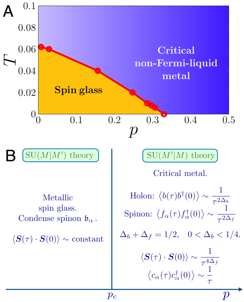
Figure 1: (A) Phase diagram as a function of doping $p$ and temperture $T$ obtained from numerically solving the fermionic spinon large $M$ saddle-point equations of the random $t$-$J$ model in Eq. 1 for $t=J=1$. The red circles are critical doping value ($p_{c}(T)$) at a given temperature, obtained by looking at the spin-glass instability in the non-Fermi-liquid solution. The uncertainty for each $p_{c}$ is within $0.003$. The critical doping at $T=0$ is obtained by directly solving the saddle-point equations on the real-frequency axis. (B) Properties of the $T=0$ states. The low-doping spin-glass phase and large-doping critical-metal phase are separated by a quantum critical point at $p_{c}$. The critical metal has doping-dependent exponents $\Delta_{f,b}$, and a linear-$T$ resistivity.

The present paper will present a full numerical solution of these large $M$ saddle point equations for a wide range of doping. The solutions are obtained on both the real and imaginary frequency axes, with mutually consistent results. We also supplement the numerical results with asymptotic analytic analyses. Our main results are that the Fermi liquid is never the solution of the large-$M$ saddle-point equations, and that one of the low energy critical solutions obtained earlier (15) extends to an all-energy solution of the large-$M$ equations in the entire overdoped regime. We further show that there is a phase transition to a low-doping spin-glass phase and construct a phase diagram (see Fig. 1).

Notable features of the novel critical non-Fermi liquid phase in Fig. 1 are
(i) spin correlations decay with an exponent which varies continuously with doping (unlike a Fermi liquid),
(ii) the electron correlators have the $\sim 1/\tau$ decay with imaginary time (as in a Fermi liquid), but with a pronounced particle-hole asymmetry (which is weak in a Fermi liquid), and
(iii) the mechanism of Ref. (16) applies across the entire overdoped critical phase, and the resistivity has a linear-$T$ contribution as $T\rightarrow 0$ at all dopings in this phase (unlike the $T^{2}$ resistivity in a Fermi liquid).

We also note here that there is a distinct large $M$ limit of the random $t$-$J$ model (17) which yields a Fermi liquid ground state at all non-zero doping. We will discuss the relation to this limit in Section 4.

The plan of the paper is as follows. In Section 1 we introduce the model and discuss its general properties. In Section 2 we consider the critical solutions of the model introduced in Eq. 1, and show that there is a critical solution with doping-dependent exponents in the overdoped region. We then solve this model at zero temperature (Section 2.2.1), as well as finite temperature (Section 2.2.2), and show that it has an instability to a spin-glass phase. The results for spectral functions in the spin-glass phase are presented in Section 3 using an alternative bosonic spinon large $M$ limit. In both phases we report physical observables such as electron and spin spectral densities at both zero and finite temperatures. We conclude with a discussion and implication of our results in Section 4. Technical details and additional results are presented in the appendices.

1 Model

We consider a model of electrons with random and all-to-all hopping and exchange interaction with double occupancy being prohibited. This is the random $t$-$J$ model which considers doping a random Heisenberg magnet (10). It is in the class of SYK models (10, 11) and is suitable for studying metallic phases obtained upon doping a Mott insulator. The Hamiltonian is

$$H=\frac{1}{\sqrt{N}}\sum_{i\neq j=1}^{N}t_{ij}c_{i\alpha}^{\dagger}c_{j\alpha}+\frac{1}{\sqrt{N}}\sum_{i<j=1}^{N}J_{ij}\vec{S}_{i}\cdot\vec{S}_{j}-\mu\sum_{i}c_{i\alpha}^{\dagger}c_{i\alpha}\,,$$ (1)

with the constraint, $\sum_{\alpha}c_{i\alpha}^{\dagger}c_{i\alpha}\leq 1$, since double occupancy is not allowed. In the above Hamiltonian, $c_{\alpha}$ is the electron annihilation operator with $\alpha=\uparrow\,,\downarrow$, the spin operator is $S_{i}^{a}=c_{i\alpha}^{\dagger}\sigma^{a}_{\alpha\beta}c_{i\beta}/2$, and $\mu$ is the chemical potential. The complex hoppings $t_{ij}$ and real exchange interactions $J_{ij}$ are independent random numbers with zero mean and mean-square values $t^{2}$ and $J^{2}$ respectively.

Note that one could also consider a $t$-$J$ model with non-random nearest-neighbor hopping and nearest-neighbor random exchange interactions on a large dimensional lattice. The on-site dynamical mean-field equations for such a model are the same as those obtained for the model in Eq. 1. It also allows for a definition of transport quantities such as resistivity.

We will consider the problem at finite hole doping ($p$). This was recently studied both analytically (15, 18) and numerically (19, 20). In particular, a deconfined critical point scenario was proposed in Ref. (15) to describe a quantum phase transition between a spin-glass phase at low doping with carrier density $p$ and a Fermi-liquid phase at large doping with carrier density $1+p$. The deconfined critical point proposed therein had the property that the local spin susceptibility was marginal as in the SYK models (10, 11). This was based on renormalization group arguments. However, a large-$M$ analysis (15) led to two types of critical metallic solutions. One of the critical solutions corresponds to the deconfined critical point (although it is a phase in large-$M$ limit), while the other was believed to be suppressed in favor of a Fermi-liquid phase.

In this work we find that, in fact, the second critical solution is stable, and a Fermi-liquid phase is never achieved within a large-$M$ approach at the saddle-point level. This critical phase has the property that while the exponent of the spin correlation continuously varies with doping, the linear-$T$ resistivity is present over the entire overdoped phase. This makes it an attractive candidate for the overdoped phase of cuprate in the light of recent experiments (5, 7). In the underdoped region, below a critical doping $p_{c}$, we find a spin-glass phase. Thus, the critical metal at large doping and spin-glass phase at small doping are separated by a quantum critical point at a finite doping $p_{c}$, as shown in Fig. 1.

As a result of the double-occupancy constraint each site has three states, namely empty ($\left|0\right\rangle$) and singly-occupied ($\left|\uparrow\right\rangle$ and $\left|\downarrow\right\rangle$) states. These can be conveniently described using holon and spinon operators. The electron is thus fractionalized into holon and spinons. The critical metallic solutions in the overdoped region has gapless and critical fermionic spinons and bosonic holons (Section 2), while the underdoped spin-glass phase will be described by a fermionic holon and bosonic spinons (Section 3).

2 Critical non-Fermi-liquid metal phase

In this section, we show that our model in Eq. 1 admits a critical metallic solution. This phase is described by fermionic spinon ($f_{\alpha}$) and bosonic holon ($b$) operators. The electron and spin operators can be then written in terms of these fractional particles as

$$c_{i\alpha}=b^{\dagger}f_{i\alpha}\,,\leavevmode\nobreak\ \leavevmode\nobreak\ S^{a}_{i}=f_{i\alpha}^{\dagger}\frac{\sigma^{a}_{\alpha\beta}}{2}f_{i\beta}\,,$$ (2)

with the constraint, $f_{i\alpha}^{\dagger}f_{i\alpha}+b_{i}^{\dagger}b_{i}=1$. This theory realizes a SU$(1|2)$ superalgebra. The strategy to solve the model in Eq. 1 is to generalize to a larger symmetry. The spin index on the spinon operator ($f_{\alpha}$) is generalized to $\alpha=1,\ldots,M$ and there is an additional orbital index for holon ($b_{\ell}$) such that $\ell=1,\ldots,M^{\prime}$. This theory realizes a SU$(M^{\prime}|M)$ superalgebra. In this larger symmetry the electron and spin operators take the form,

$$c_{\ell\alpha}=b^{\dagger}_{\ell}f_{i\alpha}\,,\leavevmode\nobreak\ \leavevmode\nobreak\ S^{a}=f_{\alpha}^{\dagger}T^{a}_{\alpha\beta}f_{\beta}\,,$$ (3)

where the matrices $T^{a}$ obey SU$(M)$ algebra. The constraint now takes the general form,

$$f_{\alpha}^{\dagger}f_{\alpha}+b_{\ell}^{\dagger}b_{\ell}=\kappa M\,.$$ (4)

The idea is to take a large-$M^{\prime},M$ limit such that $k=M^{\prime}/M$ is finite. This large $M$ limit is taken after we have performed a disorder average, and taken the large-volume limit. Note that this large $M$ limit is distinct from the large $M$ limit in Ref. (17), which had $M^{\prime}=1$; the latter limit leads to a Fermi liquid phase at $T=0$ at all non-zero doping.

A detailed analysis of our large $M$ limit can be found in Refs. (15, 18) and here we simply recall the saddle-point equations derived therein, which are

$$G_{b}(i\omega_{n})=\frac{1}{i\omega_{n}+\mu_{b}-\Sigma_{b}(i\omega_{n})},$$ (5)

$$\Sigma_{b}(\tau)=-t^{2}G_{f}(\tau)G_{f}(-\tau)G_{b}(\tau),$$ (6)

$$G_{f}(i\omega_{n})=\frac{1}{i\omega_{n}+\mu_{f}-\Sigma_{f}(i\omega_{n})},$$ (7)

$$\Sigma_{f}(\tau)=-J^{2}G_{f}(\tau)^{2}G_{f}(-\tau)+kt^{2}G_{f}(\tau)G_{b}(\tau)G_{b}(-\tau),$$ (8)

where $G_{b}$ and $G_{f}$ are the boson and fermion Green’s function respectively, while $\Sigma_{b}$ and $\Sigma_{f}$ are the boson and fermion self energies respectively. Here $\tau$ is the imaginary time and $\omega_{n}$ are the Matsubara frequencies. The chemical potentials $\mu_{f}$ and $\mu_{b}$ are chosen to satisfy

$$\left\langle f^{\dagger}f\right\rangle=\kappa-kp\quad,\quad\left\langle b^{\dagger}b\right\rangle=p\,.$$ (9)

We will restrict our attention to the physical case, $\kappa=1/2$ and $k=1/2$. In terms of the holon and spinon Green’s functions, the electron Green’s functions and the spin correlator are,

$$G_{c}(\tau)=-\langle T_{\tau}c_{\alpha}(\tau)c^{\dagger}(0)\rangle=-G_{f}(\tau)G_{b}(-\tau)$$ (10)

$$\chi(\tau)=\langle\vec{S}(\tau)\cdot\vec{S}(0)\rangle=-G_{f}(\tau)G_{f}(-\tau)\,.$$ (11)

Similar equations have been obtained by a dynamic mean field theory of a non-random $t$-$J$ model on the square lattice using a ‘non-crossing’ approximation, and studied numerically (12, 13).

To solve the saddle-point equations on the imaginary-frequency axis, it is convenient to define

$$\beta\overline{r}=-G_{b}(i\omega_{n}=0)\,.$$ (12)

Then we can eliminate $\mu_{b}$ and obtain the following set of equations to solve

$$G_{b}(i\omega_{n})=\frac{1}{i\omega_{n}-1/(\beta\overline{r})-\Sigma_{b}(i\omega_{n})+\Sigma_{b}(i\omega_{n}=0)}$$ (13)

$$\Sigma_{b}(\tau)=-t^{2}G_{f}(\tau)G_{f}(-\tau)G_{b}(\tau)$$ (14)

$$G_{f}(i\omega_{n})=\frac{1}{i\omega_{n}+\mu_{f}-\Sigma_{f}(i\omega_{n})}$$ (15)

$$\Sigma_{f}(\tau)=-J^{2}G_{f}(\tau)^{2}G_{f}(-\tau)+kt^{2}G_{f}(\tau)G_{b}(\tau)G_{b}(-\tau)$$ (16)

$$-G_{b}(\tau=0^{-})=p$$ (17)

$$G_{f}(\tau=0^{-})=\kappa-kp$$ (18)

Thus we have 6 equations to solve for the 6 variables $\overline{r}$, $\mu_{f}$, $G_{f}$, $G_{b}$, $\Sigma_{f}$, $\Sigma_{b}$. Note that Eq. 13 holds for all $\omega_{n}$.

2.1 Real-frequency solution at zero temperature

In this section we discuss the solutions of the saddle-point equations on the real-frequency axis at $T=0$. The details of real-frequency equations corresponding to Eqs. 13-18 can be found in SI Appendix LABEL:sec:REALFL. We look for a low-frequency conformal solution for the fermion and boson Green’s functions with the following form:

$$G_{a}(i\omega_{n})=-iC_{a}\begin{pmatrix}e^{-i\theta_{a}}\\ -e^{i\theta_{a}}\end{pmatrix}\frac{1}{|\omega|^{1-2\Delta_{a}}}\,,$$ (19)

where the subscript $a=f,b$ corresponds to the fermion and boson Green’s function respectively. In the above ansatz, $C_{a}$ is a constant, $\theta_{a}$ is an asymmetry parameter, and $\Delta_{a}$ is the exponent determining the critical solution. Below we shall discuss the relation between these parameters and different possible solutions. The vector notation is introduced to denote the positive and negative frequency parts of the solution. Using this form of the Green’s function it is then straightforward to write the corresponding spectral densities,

$$\rho_{a}(\omega) =-\frac{1}{\pi}\text{Im}[G_{a}(i\omega_{n}=\omega+i0^{+})]$$

$$=\frac{C_{a}}{\pi}\begin{pmatrix}\sin(\pi\Delta_{a}+\theta_{a})\\ \sin(\pi\Delta_{a}-\theta_{a})\end{pmatrix}\frac{1}{|\omega|^{1-2\Delta_{a}}}\,.$$ (20)

The exponents of the fermion and boson Green’s functions satisfy the constraint $\Delta_{f}+\Delta_{b}=1/2$. The ansataz considered in Eq. 19 admits three types of solutions (15):

(i) $\Delta_{f}=\Delta_{b}=1/4$: This is the solution that leads to a marginal spin correlation, i.e., a $1/\tau$ decay as in the SY spin liquid (10) found in the insulating case. In Ref. (18) it was shown that such a solution exists only in a very small doping range near $p=0$. This is also the solution that corresponds to the deconfined critical point discussed in Ref. (15). We will not discuss this solution any further here, because we believe the actual ground state at very low doping is a spin glass.

(ii) $\Delta_{b}=0\,,\Delta_{f}=1/2$: Such a solution would be the analog of the Fermi liquid solution found in the large $M$ limit of Ref. (17). However, it turns out that such a solution is not a valid solution of the saddle-point equations of the large $M$ limit considered here. We provide more details in SI Appendix 1.LABEL:sec:fl in this regard.

(iii) $1/4<\Delta_{f}<1/2$: In this solution the $J$ term in the fermion self-energy in Eq. 16 is sub-dominant at low energies, although it does have contributions at higher energies. This solution results in doping-dependent exponents. As we shall see below, we find this solution to be present for all values of doping, and it will be a valid solution in the overdoped region. Our subsequent analyses in this section will focus on this solution.

We now briefly discuss our strategy to find the solution (iii) and more details can be found in SI Appendix LABEL:sec:REALFL. The conformal solution ansataz introduced in Eq. 19 satisfies two Luttinger constraints (15, 18),

$$\frac{\theta_{f}}{\pi}+\left(\frac{1}{2}-\Delta_{f}\right)\frac{\sin(2\theta_{f})}{\sin(2\pi\Delta_{f})} =\frac{1}{2}-\kappa+kp\,,$$

$$\frac{\theta_{b}}{\pi}+\left(\frac{1}{2}-\Delta_{b}\right)\frac{\sin(2\theta_{b})}{\sin(2\pi\Delta_{b})} =\frac{1}{2}+p\,.$$ (21)

For solution (iii) the constants $C_{f}$ and $C_{b}$ can not be determined individually but their product is a constant. This leads to another constraint involving $\theta^{\prime}s$ and $\Delta^{\prime}s$ as shown in Ref. (15),

$$k=-\frac{\Gamma(2-2\Delta_{f})\Gamma(2\Delta_{f})\sin(\pi\Delta_{f}+\theta_{f})\sin(\pi\Delta_{f}-\theta_{f})}{\Gamma(2-2\Delta_{b})\Gamma(2\Delta_{b})\sin(\pi\Delta_{b}+\theta_{b})\sin(\pi\Delta_{b}-\theta_{b})}\,,$$ (22)

where $k=1/2$ in our case. Together with the constraint $\Delta_{f}+\Delta_{b}=1/2$ and Eqs. 2.1-22, there are four equations to solve for four variables, namely $\Delta_{f}$, $\Delta_{b}$, $\theta_{f}$, and $\theta_{b}$, at a fixed doping $p$. Solving these equations gives us these parameters as a function of doping, as shown in Fig. 2 and Fig. LABEL:fig:vals. Determination of the constants $C_{f}$ and $C_{b}$ requires full solution of the saddle point equation at all frequencies, and the resulting values are shown in Fig. LABEL:fig:vals. Of particular interest is the doping dependence of $\Delta_{b}$, shown in Fig. 2.

In the large-$M$ limit, from Eq. 11 it is clear that the anomalous dimension of the electron operator is $\eta_{c}=2(\Delta_{f}+\Delta_{b})=1$ and that of the spin operator is $\eta_{S}=4\Delta_{f}=2-4\Delta_{b}$. Therefore, from Eq. 11, as a function of the imaginary time the electron Green’s function and the local spin correlation have the form,

$$G_{c}(\tau)\sim\frac{1}{\tau}\,,\leavevmode\nobreak\ \leavevmode\nobreak\ \leavevmode\nobreak\ \leavevmode\nobreak\ \chi(\tau)\sim\frac{1}{\tau^{2-4\Delta_{b}}}\,.$$ (23)

Thus we find that although the electron Green’s function is Fermi-liquid like the spin correlation is not. Therefore the solution we have found is a critical metallic phase with a doping-dependent exponent of the spin correlation. Only in the limit $p\to 1$ we have $\Delta_{b}\to 0$, leading to a Fermi-liquid like spin correction with a $1/\tau^{2}$ decay.

Having established the presence of solution (iii), we now solve the saddle-point equations on the real-frequency axis numerically to obtain the full $\omega$ dependence of the boson and fermion spectral densities. Using these we can also obtain the electron and spin spectral densities. Fig. LABEL:fig:rf_rb shows the full $\omega$-dependent solution for the fermion and boson spectral densities, while in Fig. 3 we plot the electron and spin spectral densities. The boson and fermion spectral densities have the form $\rho_{a}(\omega)\sim\omega^{2\Delta_{a}-1}$ with $a=f,b$. Since $\Delta_{a}<1/2$, we plot the rescaled spectral densities in Fig. LABEL:fig:rf_rb. Note that the fermion and boson spectral densities are not observable quantities. However, the electron and spin spectral densities are observable in photoemission and neutron scattering experiments. These are defined as follows:

$$\rho_{c}=-\frac{1}{\pi}\mbox{Im}[G_{c}(i\omega\to\omega+i0^{+})]$$ (24)

$$\rho_{s}=\frac{1}{\pi}\mbox{Im}[\chi(i\omega\to\omega+i0^{+})]=\frac{1}{\pi}\chi^{\prime\prime}(\omega)\,.$$ (25)

In SI Appendix LABEL:sec:REALFL we present more details on evaluating these spectral densities.

As noted above, the most striking feature of our solution is a continuously varying spin-correlation exponent. This is clearly seen in Fig. 2A which shows the exponent of the spin correlator $\chi(\tau)\sim 1/|\tau|^{\eta_{s}}$ where $\eta_{s}=4\Delta_{f}$, and in Fig. 3B, where $\chi^{\prime\prime}(\omega)\sim\text{sgn}(\omega)|\omega|^{4\Delta_{f}-1}$ at low frequencies. Only in the limit $p\to 1$, we see a Fermi-liquid like behavior, $\chi^{\prime\prime}(\omega)\sim\omega$, as $\Delta_{f}\to 1/2$. The electron spectral density is a constant in the low-frequency limit with different values for $\omega\to 0^{+}$ and $\omega\to 0^{-}$ (see Fig. 3A), thus resulting in a discontinuity at $\omega=0$. It clearly displays a particle-hole asymmetry throughout this phase, which is relevant in the context of understanding the measurement of Seebeck coefficient in recent experiments (21, 22).

As for the SYK model (14), the conformal solutions to Eqs. 5-8 have time reparameterization symmetry when the self-energies are singular so that $G_{f,b}(i\omega_{n})\Sigma_{f,b}(i\omega_{n})\approx-1$. Ref. (16) discussed a mechanism relating the time reparameterization symmetry to a linear-$T$ contribution to the resistivity, and the same mechanism applies to the cases (i) and (iii) above. Briefly, to obtain a model with spatial structure, we consider the $t$-$J$ model on a large dimension lattice with non-random $t_{ij}$ but random nearest-neighbor $J_{ij}$. In the limit of large dimension, the self-energies become local, and the Green’s functions and self-energies obey equations closely related to Eqs. 5-8. The conductivity in this large dimension model is given by the Kubo formula applied at one loop to the electron Green’s function. The identity $\Delta_{f}+\Delta_{b}=1/2$ implies that $G_{c}\sim 1/\tau$, and inserting this leading scaling behavior into the Kubo formula leads to a $T$-independent residual resistivity. To obtain temperature dependence, we consider the corrections to scaling from the time reparameterization operator, whose scaling dimension $h=2$ leads to corrections which depend linearly on $T$ or $\omega$. Applying such a correction to the residual resistivity, we obtain a linear-in-$T$ resistivity. The critical metal phase found here is therefore an attractive candidate for the overdoped cuprates. We also note that our solution is consistent with the findings of recent numerical work on a similar model (20), as we will discuss further in Section 4.

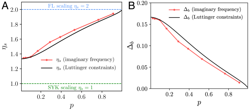
Figure 2: (A) We plot the doping dependence of the exponent $\eta_{s}$ of the spin correlation $\chi(\tau)\sim 1/|\tau|^{\eta_{s}}$. We compute $\eta_{s}=2-4\Delta_{b}$ in two independent ways, one by solving the Luttinger relations and the zero-frequency saddle point equations at $T=0$ as explained in the text (black curve) and by computing $\eta_{s}$ from the value of $\Delta_{b}$ obtained from the imaginary-frequency numerics (red curve), as discussed in Section 2.2.2. We find the two results in good agreement. At $p=0$ we obtain $\eta_{s}=4/3$, with $\eta_{s}$ increasing monotonically with increasing doping such that $\eta_{s}\to 2$ as $p\to 1$. (B) We plot the doping dependence of $\Delta_{b}$ as obtained independently from the luttinger relations and $T=0$ zero-frequency saddle point equations and from solving the imaginary frequency saddle point equations. We find at $p=0$ $\Delta_{b}=1/6$ and $\Delta_{b}\to 0$ as $p\to 1$. Consequently, this means $\Delta_{f}=1/3$ at $p=0$ and $\Delta_{f}\to 1/2$ as $p\to 1$.

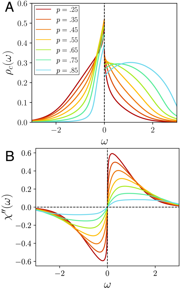
Figure 3: Plot of the electron spectral density (left) and spin spectral density (right) obtained at $t=J=1$. The electron spectral density which discontinuously approaches two different constants $\omega=0$, leading to $1/\tau$ decay of the electron density in imaginary time. The spin spectral density goes as $\text{sgn}(\omega)|\omega|^{4\Delta_{f}-1}$ as $\omega\rightarrow 0$. Only for large $p$ do we have $\Delta_{f}$ approach 1/4, which implies a linear frequency dependence and $1/\tau^{2}$ decay behavior in imaginary time characteristic of a Fermi liquid.

2.2 Imaginary-frequency solution

We also numerically solve Eqs. 13-18 on the imaginary-frequency axis at finite temperatures and for different doping values. A critical metallic solution is found for all values of doping. We calculate the parton Green’s functions as well as gauge-invariant observables, namely, electron Green’s function and spin correlation. These are shown in Fig. 4. The exponent of the bosonic Green’s function, $\Delta_{b}$, introduced in Eq. 19 can be determined from the temperature dependence of $G_{b}(i\omega=0)$. In the low-temperature limit, the bosonic Green’s function of the critical metallic solution has a conformal form at low frequencies, which follows the relation

$$G_{b}(i\omega=0)=C_{0}T^{-1+2\Delta_{b}}\,,$$ (26)

where $C_{0}$ is some constant and $T$ is the temperature. In order to extract $\Delta_{b}$ from the data, we plot $\log(G_{b}(i\omega=0))$ as a function of $\log(T)$ and perform a linear fit. The slope of this linear fit then determines $\Delta_{b}$. In Fig. 2 we plot $\Delta_{b}$ determined from this procedure as a function of doping. It is in good agreement with the result obtained from analytic solution (shown as black curve in Fig. 2) discussed in Section 2.2.1. The lowest temperature that we used for the procedure is $T=0.01$.

In the SI Appendix LABEL:sec:imag_app we present additional results obtained from solving the saddle-point equations on the imaginary-frequency axis. In particular, we calculate the electron Green’s function and the spin correlation, which are physical observables. We find that the spin correlation $\chi(\tau)$ fits the conformal form to a very high accuracy and this allows us to extract the corresponding exponent. Moreover, using Pade approximation, we also perform a numerical analytic continuation to the real-frequency axis to obtain the electron and spin spectral densities. These are discussed in SI Appendix 2.LABEL:sec:nac, and are in remarkable agreement with those obtained from real-frequency analysis at zero temperature.

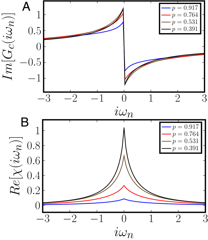
Figure 4: (A) Imaginary part of the electron Green’s function on the Matsubara-frequency axis at $T=0.01$ for different dopings. (B) Real part of the spin correlation on the Matsubara-frequency axis at $T=0.01$ for different dopings. We have used $t=J=1$.

2.3 Instability to spin-glass phase/quantum critical point

The critical metallic solution discussed above is expected to be stable at large doping values. In the low doping region we expect a spin-glass phase, which is connected to the spin-glass phase found in the insulating case (23). The critical metallic phase and the spin-glass phase are separated by a quantum critical point at a finite doping. The critical value of doping can be estimated using a Ginzburg-Landau type free energy considered in Ref. (23). It was derived by considering fluctuations over the saddle point leading to a $1/M$ correction and it has a form,

$$\mathcal{F}=\left[1-\frac{J^{2}}{M}\chi^{2}(i\omega=0)\right]\Psi^{2}+\ldots\,,$$ (27)

where $\chi(i\omega=0)=\int_{0}^{\beta}\chi(\tau)d\tau$ is the local spin susceptiblity and $\Psi$ is the spin-glass order parameter. In the insulating $p=0$ phase studied in Ref. (23), it was found that $\chi(i\omega=0)$ diverged logarithmically at $T=0$ because the spin exponent has the ‘marginal’ value $\eta_{s}=1$. Consequently the co-efficient of $\Psi^{2}$ is always negative as $T\rightarrow 0$, and spin glass order is present at $T=0$. In our non-Fermi liquid solution, $\eta_{s}<1$, and so $\chi(i\omega=0)$ is finite at $T=0$: this allows the possibility of $\Psi=0$ and no spin glass order at $T=0$. We find in the overdoped region the coefficient of the quadratic term is positive and the free energy is thus minimized by $\Psi=0$. On the other hand, in the underdoped region this coefficient is negative leading to a non-zero spin-glass order parameter. A change in the sign of the coefficient of $\Psi^{2}$ at $T=0$ thus indicates a quantum phase transition to a spin-glass phase and can be used to estimate the critical value of doping. We plot this coefficient at zero temperature in Fig. 5A as a function of doping for different values of $J$ at $M=2$. We clearly see that for larger values of $J$ there is a quantum phase transition at a finite doping. In particular, for $J=1$ we find $p_{c}\approx 0.33$ and for $J=0.5$ we get $p_{c}\approx 0.25$. Similarly, in Fig. 5B we plot the coefficient in Eq. 27 as a function of doping for different values of $M$ at a fixed $J=1$ at zero temperature. It is clear that for large values of $M$ there is no phase transition. We also plot the critical value of $M$ as a function of doping in Fig. 6 at zero temperature. We perform a similar analysis at finite temperature to obtain the critical doping as a function of temperature (see Fig. LABEL:fig:c_p). The resulting phase diagram is shown in Fig. 1A. The spin-glass susceptibility increases with decreasing temperature and thus the spin-glass phase is found upon cooling the non-Fermi liquid at low doping. However, note that unlike in the case of the random Heisenberg model (10, 24) (where the solution $(i)$ with $\Delta_{f}=\Delta_{b}=1/4$ is present) the spin-glass susceptibility does not diverge at low temperature in the present case. This is one of the important reasons for a stable critical solution at zero temperature in a broad doping region. We also note that while $1/M$ corrections are used in deriving the form of Eq. 27, we have used the $M\rightarrow\infty$ solution for the critical metal to compute $\chi^{\prime}(0)$ as it appears in Eq. 27. While a more accurate estimate of $p_{c}$ may be obtained by adding $1/M$ corrections to the critical metal solution, we emphasize that the $M\rightarrow\infty$ solution is sufficient to capture existence of a finite doping phase transition between the spin glass and critical metal.

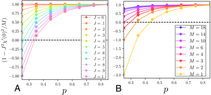
Figure 5: Plots of the coefficient of the quadratic term in the free energy in Eq. 27 as a function of doping for (A) different values of $J$ with $t=1$ and $M=2$; (B) different values of $M$ with $t=J=1$. In both plots, $T=0$.

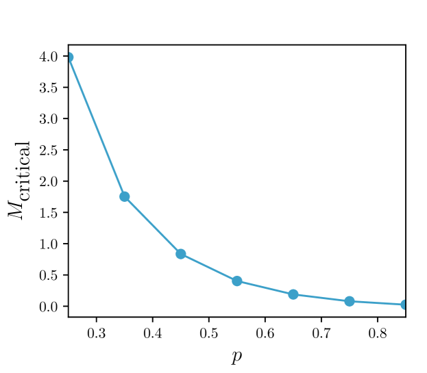
Figure 6: Plot showing critical value of $M$ for which coefficient of quadratic term in free energy Eq. 27 changes sign at zero temperature.

3 Spin-glass phase

In this section we discuss the spin-glass phase present at lower dopings. In this case, we shall use the representation where spinons are bosonic ($\mathfrak{b}$) and holon is a fermion operator ($\mathfrak{f}$). In terms of these operators,

$$c_{\alpha}=\mathfrak{f}^{\dagger}\mathfrak{b}_{\alpha}\,,\leavevmode\nobreak\ \leavevmode\nobreak\ \leavevmode\nobreak\ \leavevmode\nobreak\ \vec{S}=\mathfrak{b}^{\dagger}_{\alpha}\frac{\vec{\sigma}_{\alpha\beta}}{2}\mathfrak{b}_{\beta}\,,$$ (28)

and we realize a SU$(2|1)$ superalgebra. Just as before, we shall now enlarge the symmetry here to SU$(M|M^{\prime})$, which means $\alpha=1,\ldots,M$ and the holon operator acquires an index $\ell=1,\ldots,M^{\prime}$. Note that this bosonic spinon large $M$ limit is distinct from the fermionic spinon large $M$ limit followed in Section 2, and the two models are the same only for $M=2$; so there is no reason to expect quantitive agreement between the results of the present section and those of Section 3.

The strategy to obtain the saddle-point equations is similar to that discussed earlier in Section 2. From Refs. (15, 18), we have

$$G_{\mathfrak{b}}(i\omega_{n})=\frac{1}{i\omega_{n}+\mu_{\mathfrak{b}}-\Sigma_{\mathfrak{b}}(i\omega_{n})}\,,$$

$$G_{\mathfrak{f}}(i\omega_{n})=\frac{1}{i\omega_{n}+\mu_{\mathfrak{f}}-\Sigma_{\mathfrak{f}}(i\omega_{n})}\,,$$

$$\Sigma_{\mathfrak{b}}(\tau)=-kt^{2}G_{\mathfrak{f}}(\tau)G_{\mathfrak{f}}(-\tau)G_{\mathfrak{b}}(\tau)+J^{2}G_{\mathfrak{b}}(\tau)^{2}G_{\mathfrak{b}}(-\tau)\,,$$

$$\Sigma_{\mathfrak{f}}(\tau)=t^{2}G_{\mathfrak{f}}(\tau)G_{\mathfrak{b}}(-\tau)G_{\mathfrak{b}}(\tau)\,,$$

$$G_{\mathfrak{b}}(\tau=0^{-})=-\kappa+kp\,,$$

$$G_{\mathfrak{f}}(\tau=0^{-})=p\,.$$

Physically, the spin-glass phase can be understood as a condensation of bosonic spinons. Contrary to the earlier case, since we are interested in the spin-glass phase we need to retain the replica off-diagonal terms in the action upon disorder averaging. There is however some simplification and only replica off-diagonal components of the bosonic Green’s function at $i\omega_{n}=0$ are relevant. These are captured via the parameter $g$ which is related to the spin-glass order parameter, as discussed in detail in SI Appendix LABEL:sec:SY. After incorporating the spin-glass order in $G_{\mathfrak{b}}(\tau)=G_{r}(\tau)-g$, we obtain the following saddle-point equations:

$$\left[G_{r}(i\omega_{n})\right]^{-1}=i\omega_{n}-\frac{Jg}{\Theta}-\left[\Sigma_{r}(i\omega_{n})-\Sigma_{r}(i\omega_{n}=0)\right]$$ (29)

$$G_{\mathfrak{f}}(i\omega_{n})=\frac{1}{i\omega_{n}+\mu_{\mathfrak{f}}-\Sigma_{\mathfrak{f}}(i\omega_{n})}\,,$$ (30)

$$\Sigma_{r}(\tau)=J^{2}\Bigl{(}\left[G_{r}(\tau)\right]^{2}G_{r}(-\tau)-2gG_{r}(\tau)G_{r}(-\tau)-g\left[G_{r}(\tau)\right]^{2}$$

$$+2g^{2}G_{r}(\tau)+g^{2}G_{r}(-\tau)\Bigr{)}-kt^{2}G_{\mathfrak{f}}(\tau)G_{\mathfrak{f}}(-\tau)\Bigl{(}-g+G_{r}(\tau)\Bigr{)},$$ (31)

$$\Sigma_{\mathfrak{f}}(\tau)=t^{2}G_{\mathfrak{f}}(\tau)\Bigl{(}g^{2}-gG_{r}(\tau)-gG_{r}(-\tau)+G_{r}(-\tau)G_{r}(\tau)\Bigr{)}\,,$$ (32)

$$g-G_{r}(\tau=0^{-})=\kappa-kp$$ (33)

$$G_{\mathfrak{f}}(\tau=0^{-})=p\,.$$ (34)

The dimensionless parameter $\Theta=1/\sqrt{3}$, as detailed in SI Appendix LABEL:sec:SY. We solve the above equations on real and imaginary-frequency axes. The main observable in this phase is the spin-glass order parameter, which we plot as a function of doping in Fig. 7 at zero temperature. The spin-glass order parameter is finite at lower dopings and decreases upon increasing doping. We show results for the order parameter computed for small but finite temperature obtained using the imaginary frequency analysis in SI Appendix LABEL:sec:imag_app_sg. We also calculate the holon and spinon Green’s functions as well as the electron Green’s function and spin correlation at finite temperature. These quantities are detailed in the same SI Appendix LABEL:sec:imag_app_sg.

We solve the saddle-point equations Eqs. 29-34 at zero temperature to obtain the fermion and boson spectral functions, as well as the electron and spin spectral functions for a range of doping. In terms of the spinon and holon spectral functions the electron spectral function has the following form:

$$\rho_{c}(\omega)=\int_{0}^{\omega}d\omega_{1}\rho_{r}(\omega_{1})\rho_{\mathfrak{f}}(\omega_{1}-\omega)+g\rho_{\mathfrak{f}}(-\omega)\,.$$ (35)

Similarly, we obtain the expression for the spin spectral function,

$$\rho_{s}(\omega) =g^{2}\beta\omega\delta(\omega)+g\left[\rho_{r}(\omega)-\rho_{r}(-\omega)\right]$$

$$-\int_{0}^{\omega}d\omega_{1}\leavevmode\nobreak\ \rho_{r}(\omega_{1})\rho_{r}(\omega-\omega_{1})\,,$$ (36)

as in Ref. (24). The spectral functions at zero temperature for different values of doping are shown in Fig. 8. We note that the boson spectral function behaves linearly with frequency at small frequencies. Consequently, the spin spectral function also depends linearly on $\omega$ at small frequencies. We also note the double peak structure in the electron spectral function $\rho_{c}(\omega)$ in Fig. 8B. Recall that the electron spectral function is a convolution of the spinon and holon spectral functions, as well as a term proportional to $g\rho_{\mathfrak{f}}(-\omega)$. At small dopings the value of $g$ is larger and hence there is a dominant peak coming from fermion spectral function. As $g$ decreases with increasing doping the contribution from the boson spectral function increases leading to the second peak at positive frequencies. All the spectral functions satisfy the respective sum rules, which are detailed in SI Appendix 4.LABEL:sec:sg_sd.

Apart from the numerical analysis at zero temperature, we also perform a Pade-approximation based numerical analytic continuation of the imaginary-axis solution obtained at finite temperature. We evaluate the holon, spinon, electron, and spin spectral densities at finite temperature. These are discussed in SI Appendix 2.LABEL:sec:nac, and are consistent with those obtained from real-frequency calculation at zero temperature for some range of doping.

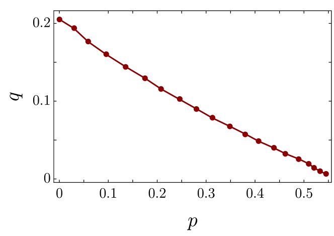
Figure 7: Plot of spin-glass order parameter, $q=g^{2}$, as a function of doping obtained by solving the bosonic spinon saddle-point equations (29 - 34) on the real-frequency axis at $T=0$. The point at $p=0$ is obtained by solving equations (LABEL:ysr14a-LABEL:ysr14c) at zero temperature on the real frequency axis. The parameters of the model are $J=t=1$. The critical doping $p_{c}$ at which the spin glass order vanishes in the present bosonic spinon computation need not be the same as that in the fermionic spinon computation in Section 2.2.3 because the models are identical only for $M=2$.

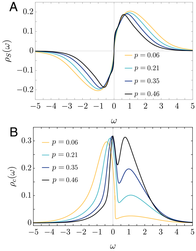
Figure 8: (A) Spin spectral function and (B) electron spectral function obtained at zero temperature via real frequency analysis for several values of doping. Note the linear in frequency behavior at small frequencies for $\rho_{S}(\omega)$. Parameters are $J=t=1$.

4 Discussion

We have presented a large-$M$ solution for the random $t$-$J$ model for the entire doping range. Our main finding is a critical non-Fermi-liquid metal phase at large dopings. This phase is characterized by a spin correlation exponent which varies continuously with doping, a linear in temperature contribution to the resistivity as $T\to 0$, and an electron spectral function with a Fermi-liquid-like decay at long time, but with a pronounced particle-hole asymmetry. This critical phase captures many aspects of experimental observations in the overdoped cuprates. It has been observed that in the overdoped region of cuprate materials there is a broad range of doping where the resistivity display a linear-$T$ behavior (5, 7). Our findings propose a possible mechanism for this observation. Also, recent Seebeck coefficient measurements (21, 22) hint towards a particle-hole asymmetric electron spectral density, which our solution also displays. It turns out that in our solution the electron Green’s function appears Fermi-liquid like although the spin correlation does not. This may also explain the fact that experiments on overdoped cuprates probing electron Green’s function directly, such as photoemission (4), may observe a Fermi-liquid behavior and can not access the critical phase. However, transport measurements obtain properties such as linear-$T$ resistivity which is starkly in contrast to a Fermi liquid.

We also show that the overdoped critical phase has an instability towards a spin-glass phase at lower dopings. The spin-glass phase is characterized by a spin-glass order parameter, which we calculate using bosonic spinons. We show that this order parameter decreases upon increasing doping. In the context of cuprates, recent experiments have reported the presence of spin-glass phase at low doping (9). Our work therefore presents a comprehensive analysis of model in Eq. 1 at variable doping and captures the quantum phase transition between the spin-glass phase and a critical non-Fermi-liquid metal. We also note that our results are consistent with recent numerical work on a related model (20).

A notable feature of our results is that we never find a Fermi-liquid phase in our large $M$ limit of the $t$-$J$ model, as discussed in SI Appendix 1.LABEL:sec:fl. This is in contrast to the distinct large $M$ limit of Ref. (17), in which the boson $b$ condenses at all non-zero $p$, leading to a Fermi-liquid phase at all doping. The two large $M$ limits co-incide only for the physical value $M=2$, and it is an open question which large $M$ limit yields the correct picture at $M=2$ for the random $t$-$J$ model. However, we will note that the numerical study of the $M=2$ case in Ref. (20) does show indications of non-Fermi liquid behavior in the overdoped regime over the $T$ range studied, as their measured spin exponent $\eta_{s}$ varies with doping in a manner consistent with Fig. 2A. Thus, although a Fermi liquid phase may eventually appear at very low $T$ in the overdoped regime for $M=2$, it does appear that our non-Fermi liquid solution is an attractive description of the physics over a wide range of temperatures and dopings accessible in numerics and experiments.

In conclusion, our work presents a critical metallic phase as an attractive candidate for the overdoped cuprates which matches observations over a significant temperature range. This phase is obtained for a model with random and all-to-all interactions. Although such a model is far from the microscopic Hamiltonian of the cuprates, the saddle point equations solved are closely related to dynamic mean field equations of more realistic models in finite dimensions (12, 13), as has been extensively discussed in a recent review (14). At very low temperatures, we ultimately expect a crossover to behavior characteristic of finite-dimensional systems, and describing this crossover remains an important topic for future research.

Acknowledgements

This research was supported by the U.S. National Science Foundation grant No. DMR-2002850 by the Simons Collaboration on Ultra-Quantum Matter which is a grant from the Simons Foundation (651440, S.S.). D.G.J. acknowledges support from the Leopoldina fellowship by the German National Academy of Sciences through grant no. LPDS 2020-01.

See pages 1 of PNAS-NFL-SI See pages 2 of PNAS-NFL-SI See pages 3 of PNAS-NFL-SI See pages 4 of PNAS-NFL-SI See pages 5 of PNAS-NFL-SI See pages 6 of PNAS-NFL-SI See pages 7 of PNAS-NFL-SI See pages 8 of PNAS-NFL-SI See pages 9 of PNAS-NFL-SI See pages 10 of PNAS-NFL-SI See pages 11 of PNAS-NFL-SI See pages 12 of PNAS-NFL-SI See pages 13 of PNAS-NFL-SI See pages 14 of PNAS-NFL-SI See pages 15 of PNAS-NFL-SI See pages 16 of PNAS-NFL-SI See pages 17 of PNAS-NFL-SI

References

- (1) C Proust, L Taillefer, The remarkable underlying ground states of cuprate superconductors. \JournalTitleAnnual Review of Condensed Matter Physics 10, 409–429 (2019).
- (2) B Michon, et al., Thermodynamic signatures of quantum criticality in cuprate superconductors. \JournalTitleNature 567, 218–222 (2019).
- (3) S Badoux, et al., Change of carrier density at the pseudogap critical point of a cuprate superconductor. \JournalTitleNature 531, 210–214 (2016).
- (4) SD Chen, et al., Incoherent strange metal sharply bounded by a critical doping in bi2212. \JournalTitleScience 366, 1099–1102 (2019).
- (5) RA Cooper, et al., Anomalous Criticality in the Electrical Resistivity of La2-xSrxCuO4. \JournalTitleScience 323, 603–607 (2009).
- (6) RL Greene, PR Mandal, NR Poniatowski, T Sarkar, The strange metal state of the electron-doped cuprates. \JournalTitleAnnual Review of Condensed Matter Physics 11, 213–229 (2020).
- (7) J Ayres, et al., Incoherent transport across the strange-metal regime of overdoped cuprates. \JournalTitleNature 595, 661–666 (2021).
- (8) C Panagopoulos, et al., Exposing the spin-glass ground state of the nonsuperconducting high- oxide. \JournalTitlePhys. Rev. B 69, 144510 (2004).
- (9) M Frachet, et al., Hidden magnetism at the pseudogap critical point of a cuprate superconductor. \JournalTitleNature Physics 16, 1064–1068 (2020).
- (10) S Sachdev, J Ye, Gapless spin-fluid ground state in a random quantum Heisenberg magnet. \JournalTitlePhys. Rev. Lett. 70, 3339 (1993).
- (11) AY Kitaev, Talks at KITP, University of California, Santa Barbara. \JournalTitleEntanglement in Strongly-Correlated Quantum Matter (2015).
- (12) K Haule, A Rosch, J Kroha, P Wölfle, Pseudogaps in an Incoherent Metal. \JournalTitlePhys. Rev. Lett. 89, 236402 (2002).
- (13) K Haule, A Rosch, J Kroha, P Wölfle, Pseudogaps in the t-J model: An extended dynamical mean-field theory study. \JournalTitlePhys. Rev. B 68, 155119 (2003).
- (14) D Chowdhury, A Georges, O Parcollet, S Sachdev, Sachdev-Ye-Kitaev Models and Beyond: A Window into Non-Fermi Liquids (2021).
- (15) DG Joshi, C Li, G Tarnopolsky, A Georges, S Sachdev, Deconfined critical point in a doped random quantum heisenberg magnet. \JournalTitlePhys. Rev. X 10, 021033 (2020).
- (16) H Guo, Y Gu, S Sachdev, Linear in temperature resistivity in the limit of zero temperature from the time reparameterization soft mode. \JournalTitleAnnals Phys. 418, 168202 (2020).
- (17) O Parcollet, A Georges, Non-Fermi-liquid regime of a doped Mott insulator. \JournalTitlePhys. Rev. B 59, 5341–5360 (1999).
- (18) M Tikhanovskaya, H Guo, S Sachdev, G Tarnopolsky, Excitation spectra of quantum matter without quasiparticles II: random - models. \JournalTitlePhys. Rev. B 103, 075142 (2021).
- (19) H Shackleton, A Wietek, A Georges, S Sachdev, Quantum Phase Transition at Nonzero Doping in a Random Model. \JournalTitlePhys. Rev. Lett. 126, 136602 (2021).
- (20) PT Dumitrescu, N Wentzell, A Georges, O Parcollet, Planckian metal at a doping-induced quantum critical point. \JournalTitlePhys. Rev. B 105, L180404 (2022).
- (21) A Gourgout, et al., Seebeck coefficient in a cuprate superconductor: particle-hole asymmetry in the strange metal phase and Fermi surface transformation in the pseudogap phase (2021).
- (22) A Georges, J Mravlje, Skewed non-Fermi liquids and the Seebeck effect. \JournalTitlePhys. Rev. Research 3, 043132 (2021).
- (23) M Christos, FM Haehl, S Sachdev, Spin liquid to spin glass crossover in the random quantum Heisenberg magnet. \JournalTitlePhys. Rev. B 105, 085120 (2022).
- (24) A Georges, O Parcollet, S Sachdev, Quantum fluctuations of a nearly critical Heisenberg spin glass. \JournalTitlePhys. Rev. B 63, 134406 (2001).