Floquet States in Open Quantum Systems

Abstract

In Floquet engineering, periodic driving is used to realize novel phases of matter which are inaccessible in thermal equilibrium. For this purpose, the Floquet theory provides us a recipe of obtaining a static effective Hamiltonian. Although many existing works have treated closed systems, it is important to consider the effect of dissipation, which is ubiquitous in nature. Understanding interplay of periodic driving and dissipation is not only a fundamental problem of nonequilibrium statistical physics, but also receiving growing interest because of the fact that experimental advances have allowed us to engineer dissipation in a controllable manner. In this review, we give a detailed exposition on the formalism of quantum master equations for open Floquet systems and highlight recent works investigating whether equilibrium statistical mechanics applies to Floquet states.

1 INTRODUCTION

Nonequilibrium states are not well understood as compared with equilibrium states, except for weakly driven systems described by the linear response theory [1]. One of the recent progresses of nonequilibrium statistical physics is a discovery of fluctuation theorems [2, 3, 4], which yield nontrivial equalities for arbitrarily far-from-equilibrium systems. Although fluctuation theorems reveal universal properties of atypical fluctuations in nonequilibrium states, they do not give much insights into typical behavior of the system.

There is another important class of nonequilibrium problems for which we have gained a deeper understanding of generic properties through recent studies, that is, periodically driven (Floquet) systems in the high-frequency regime. Nonequilibrium dynamics of closed Floquet systems have intensively been studied [5, 6]. In a closed system, the second law of thermodynamics implies that the system absorbs the energy from periodic driving and eventually heats up to an infinitely high temperature. However, it is revealed that the heating process is exponentially slow in the high-frequency regime and we can have nontrivial transient states which last in a relatively long timescale [7, 8, 9, 10]. Theoretical understanding of this phenomenon gives a solid basis for the “Floquet engineering”, which is an attempt to realize desired states by utilizing engineered periodic driving [11]. Periodic driving has been used to realize nonequilibrium phase transitions [12, 13, 14], topologically nontrivial systems [15, 16, 17, 18, 19], artificial gauge fields [20, 21, 22], and discrete time crystals [23, 24, 25].

In this review, we discuss open Floquet systems. In the context of the Floquet engineering, the motivation of considering open systems is two-fold. First, although the closed-system description would be adequate in ultracold atomic systems, where high isolation from the environment is achieved, dissipation is inevitable in condensed matter physics. Dissipation can largely affect many-body states, and hence it is clearly important to formulate the problem in an open-system setup to develop the theory of Floquet engineering in condensed matter systems [26, 27, 28, 29, 30, 31, 32]. For instance, the importance of dissipation has been pointed out in recent experimental [33] and theoretical [34] studies on the light-induced anomalous Hall effect in graphene. Second, it has been recognized that dissipation can be used as a resource for creating novel nonequilibrium states. Indeed, the balance of periodic driving and dissipation can yield a variety of nonequilibrium steady states and phase transitions in various systems including cavity-QED systems [35, 36, 37, 38, 39], cold atoms [40, 41], ideal Bose gases [42, 43, 44], and so on. This direction of research has attracted growing attention in the field of ultracold atomic physics, reflecting recent experimental development that enables us to engineer dissipation in a highly controllable manner [45, 46, 47].

The interplay of periodic driving and dissipation is also intriguing from a purely theoretical perspective. The Floquet theory tells us that a Floquet system is described by an effective static Hamiltonian, and hence it is a fundamental question to what extent the notion of equilibrium statistical thermodynamics applies to the effective Hamiltonian description of Floquet systems [48, 49, 50, 51, 52, 53, 54, 55], especially beyond the linear response regime.

The purpose of this review is to give a detailed description of theoretical formulation of open Floquet systems and an overview of recent studies on statistical mechanics for Floquet systems. The organization of this review is as follows. In section 2, we present an introduction to the Floquet theory for closed systems. We explain the method of the high-frequency expansion and discuss its generic properties. A brief exposition on recent theoretical studies is also given. In section 3, we give a detailed description of the master equation approach to open Floquet systems. We introduce several kinds of quantum master equations and discuss their limitations. In section 4, we focus on nonequilibrium periodic steady states under fast driving. Here we deal with a fundamental question to what extent the method of statistical mechanics applies. In section 5, we discuss some related recent topics and provide an outlook for future studies.

2 FLOQUET THEORY FOR CLOSED SYSTEMS

2.1 Floquet Theorem

First, let us start with discussion on how to describe Floquet systems without dissipation. We denote by $\hat{H}_{0}$ and $\hat{V}(t)$ the reference Hamiltonian and the driving field of a quantum system, respectively. We assume that $\hat{V}(t)$ is periodic, $\hat{V}(t)=\hat{V}(t+T)$, with the period $T$. Without loss of generality, we can put $\int_{0}^{T}\differential t\,\hat{V}(t)=0$. We define $\omega=2\pi/T$, which is simply called the frequency of the driving field, although the driving field is not necessarily monochromatic and generally written as $\hat{V}(t)=\sum_{m\neq 0}V_{m}e^{-im\omega t}$. The state $\ket{\psi(t)}$ of the system evolves under the Schrödinger equation

$$i\derivative{t}\ket{\psi(t)}=\hat{H}(t)\ket{\psi(t)},$$ (1)

where $\hat{H}(t)=\hat{H}_{0}+\hat{V}(t)$ and we set $\hbar=1$.

Throughout this article, we consider a local Hamiltonian, i.e., a short-range interacting system, on a regular lattice. The characteristic local energy scale is denoted by $g$. More explicitly, in a lattice system, we define $g$ as the maximum single-site energy [8, 7].

A convenient theoretical tool to deal with a set of time-periodic linear differential equations like eq. 1 is the Floquet theorem. The Floquet theorem states that the time evolution operator from time $t_{0}$ to time $t$ is written in the following form [5]:

$$\hat{U}_{t,t_{0}}=e^{-i\hat{K}(t)}e^{-i\hat{H}_{\mathrm{F}}(t-t_{0})}e^{i\hat{K}(t_{0})},$$ (2)

where $\hat{K}(t)$ is called the micromotion operator or the kick operator, which is periodic in time $\hat{K}(t)=\hat{K}(t+T)$, and $\hat{H}_{\mathrm{F}}$ is the time-independent Floquet Hamiltonian. Physically, $\hat{K}(t)$ describes fast periodic motion of the system, whereas $\hat{H}_{\mathrm{F}}$ determines the long-time behavior of the system. In closed systems, we can always choose $\hat{K}(t)$ and $\hat{H}_{\mathrm{F}}$ to be Hermitian.

Eigenstates $\quantity{\ket{u_{a}}}$ and eigenvalues $\quantity{\varepsilon_{a}}$ of $\hat{H}_{\mathrm{F}}$ are called Floquet eigenstates and quasi-energies, respectively. We also define $\ket{u_{a}(t)}=e^{-i\hat{K}(t)}\ket{u_{a}}$, which satisfies $\ket{u_{a}(t)}=\ket{u_{a}(t+T)}$. A solution of the Schrödinger equation is then written in the form $\ket{\psi(t)}=\sum_{a}c_{a}e^{-i\varepsilon_{a}t}\ket{u_{a}(t)}$, which can be regarded as an analogue of the Bloch theorem in condensed matter physics. It should be noted that quasi-energies are defined modulo $\omega$: eq. 2 does not change if we replace $\varepsilon_{a}\to\varepsilon_{a}+m\omega$ with $m$ an arbitrary integer. In literature, $\varepsilon_{a}$ is often chosen within the “first Brillouin zone”, $\varepsilon_{a}\in[-\omega/2,\omega/2)$ or $\varepsilon_{a}\in[0,\omega)$. It is also convenient to choose $\varepsilon_{a}$ so that the value of $\varepsilon_{a}$ is closest to the mean energy $\bar{E}_{a}=(1/T)\int_{0}^{T}\differential t\,\expectationvalue{\hat{H}(t)}{u_{a}(t)}$, which will be used in section 4.

By substituting eq. 2 into the Schrödinger equation $i\differential\hat{U}_{t,t_{0}}/\differential t=\hat{H}(t)\hat{U}_{t,t_{0}}$, we obtain

$$\hat{H}_{\mathrm{F}}=e^{i\hat{K}(t)}\quantity[\hat{H}(t)-i\derivative{t}]e^{-i\hat{K}(t)}.$$ (3)

This expression is equivalent to eq. 2.

We remark that the decomposition of eq. 2 is not unique: there are infinitely many variants of the decomposition, which are equivalent with each other but offer different approximation schemes. Indeed, one can confirm that eq. 2 or eq. 3 is invariant under the transformation $\hat{H}_{\mathrm{F}}^{\prime}=\hat{U}\hat{H}_{\mathrm{F}}\hat{U}^{\dagger}$ and $e^{i\hat{K}^{\prime}(t)}=\hat{U}e^{i\hat{K}(t)}$ for any unitary operator $\hat{U}$. One familiar choice is putting $\hat{K}(t_{0})=0$ for a fixed $t_{0}\in[0,T)$. In this choice, the time evolution operator over a cycle $U_{t_{0}+T,t_{0}}=\mathcal{T}e^{-i\int_{t_{0}}^{t_{0}+T}\differential t\,\hat{H}(t)}$, where $\mathcal{T}$ denotes the time-ordering operation, is expressed as $\hat{U}_{t_{0}+T,t_{0}}=e^{-i\hat{H}_{\mathrm{F}}T}$. Thus, $\hat{H}_{\mathrm{F}}$ exactly describes stroboscopic evolution, which is defined at $t=t_{0}+nT$ with $n$ being an integer.

2.2 High-Frequency Expansion

Although the decomposition of eq. 2 is exact, it is hard to calculate $\hat{H}_{\mathrm{F}}$ and $\hat{K}(t)$. It is also difficult to gain some insights into the nonequilibrium dynamics from $\hat{K}(t)$ and $\hat{H}_{\mathrm{F}}$ since no analytic expression is available.

In the high-frequency regime, we can obtain approximate analytic expressions via the method of the high-frequency expansion, which is written in the form

$$\hat{K}(t)=\sum_{k=1}^{\infty}\frac{\hat{\Lambda}_{k}(t)}{\omega^{k}}\mbox{\quad and\quad}\hat{H}_{\mathrm{F}}=\hat{H}_{0}+\sum_{k=1}^{\infty}\frac{\hat{\Omega}_{k}}{\omega^{k}}.$$ (4)

By substituting eq. 4 into eq. 3, we can determine $\hat{\Lambda}_{k}(t)$ and $\hat{\Omega}_{k}$ order by order.

Reflecting the non-uniqueness of $\hat{K}(t)$ and $\hat{H}_{\mathrm{F}}$, there are several high-frequency expansions [56]. A familiar one is the high-frequency expansion with the boundary condition $\hat{K}(t_{0})=0$, which is referred to as the Floquet-Magnus expansion [57]. In the order of $\omega^{-1}$, we have

$$\hat{\Lambda}_{1}^{\mathrm{FM}}(t)=i\sum_{m\neq 0}\frac{\hat{V}_{m}}{m}\quantity(e^{-im\omega t}-e^{-im\omega t_{0}}),\quad\hat{\Omega}_{1}^{\mathrm{FM}}=\sum_{m\neq 0}\frac{[\hat{V}_{-m},\hat{V}_{m}]}{2m}+\sum_{m\neq 0}\frac{[\hat{V}_{m},\hat{H}_{0}]}{m}e^{-im\omega t_{0}}.$$ (5)

It should be noted that the high-frequency expansion of $\hat{H}_{\mathrm{F}}$ depends on $t_{0}$, which is sometimes not desirable because we are interested in the long-time physics independent of the particular choice of $t_{0}$. We can also construct the high-frequency expansion so that this undesirable $t_{0}$ dependence is completely removed. It is known as the van Vleck expansion [58, 59, 60] and characterized by the boundary condition $\int_{0}^{T}\differential t\,\hat{K}(t)=0$. In the order of $\omega^{-1}$, the van Vleck expansion is given by

$$\hat{\Lambda}_{1}^{\mathrm{vV}}(t)=i\sum_{m\neq 0}\frac{\hat{V}_{m}}{m}e^{-im\omega t},\quad\hat{\Omega}_{1}^{\mathrm{vV}}=\sum_{m\neq 0}\frac{\quantity[\hat{V}_{-m},\hat{V}_{m}]}{2m}.$$ (6)

Since analytic expressions of $\hat{\Omega}_{k}$ and $\hat{\Lambda}_{k}(t)$ are available, the high-frequency expansion provides us much insights into long-time dynamics of Floquet systems. A generic strategy of the Floquet engineering is to engineer periodic driving so that a truncation of the Floquet Hamiltonian

$$\hat{H}_{\mathrm{F}}^{(n)}=\hat{H}_{0}+\sum_{k=1}^{n}\frac{\hat{\Omega}_{k}}{\omega^{k}}$$ (7)

has a desired property [11].

It should be noted that if we simply increase the frequency, the leading-order term in eq. 4 is dominant and thus we approximately have $\hat{H}_{\mathrm{F}}^{(n)}\approx\hat{H}_{0}$: the periodic driving does not play any role. In order to realize nontrivial states by using fast periodic driving, we should either (i) strongly or (ii) resonantly drive the system, which we explain in the following.

2.2.1 Strong Driving

Let us consider a class of periodic fields of the form $\hat{V}(t)=\omega f(\omega t)\hat{V}$, where $\hat{V}$ is a time-independent operator and $f(\omega t)$ is an arbitrary periodic function satisfying $f(\theta)=f(\theta+2\pi)$ and $\int_{0}^{2\pi}\differential\theta\,f(\theta)=0$. A monochromatic driving $f(\omega t)=\cos(\omega t)$ is often used. Since the driving amplitude scales with $\omega$, a large $\omega$ compared with a local energy scale $g$ of $\hat{H}_{0}$ corresponds to fast and strong driving. The Hamiltonian is given by

$$\hat{H}(t)=\hat{H}_{0}+\omega f(\omega t)\hat{V}.$$ (8)

Under such a strong driving field, the convergence of the high-frequency expansion is very slow. This difficulty is addressed by moving to a rotating frame via the unitary transformation $e^{-i\int_{0}^{t}\differential s\,\hat{V}(s)}=e^{-iF(\omega t)\hat{V}}$ with $F(\theta)=\int_{0}^{\theta}\differential s\,f(s)$. The Hamiltonian in the rotating frame is given by

$$\hat{H}^{\mathrm{R}}(t)=e^{-iF(\omega t)\hat{V}}\hat{H}_{0}e^{iF(\omega t)\hat{V}}=\hat{H}_{0}^{\mathrm{R}}+\hat{V}^{\mathrm{R}}(t),$$ (9)

where $\hat{H}_{0}^{\mathrm{R}}=(1/T)\int_{0}^{T}\differential t\,\hat{H}^{\mathrm{R}}(t)$ and $\hat{V}^{\mathrm{R}}(t)$ are the static Hamiltonian and the driving field in the rotating frame, respectively. It is emphasized that $\hat{H}_{0}^{\mathrm{R}}$ contains nonperturbative effects of periodic driving. Since $\hat{H}^{\mathrm{R}}(t)=\hat{H}^{\mathrm{R}}(t+T)$ is satisfied, the Floquet theory is still applicable in the rotating frame. Remarkably, the periodic driving in the rotating frame is no longer strong. It is therefore expected that the high-frequency expansion quickly converges. The static part $\hat{H}_{0}^{\mathrm{R}}$ gives the leading order term of the high-frequency expansion of the Floquet Hamiltonian.

This technique has been used for Floquet engineering. As an example, let us consider a one-dimensional Bose-Hubbard system in a shaken optical lattice [12]:

$$\hat{H}_{0}=-J\sum_{j=1}^{L-1}\quantity(\hat{b}_{j+1}^{\dagger}\hat{b}_{j}+\hat{b}_{j}^{\dagger}\hat{b}_{j+1})+\frac{U}{2}\sum_{j=1}^{L}\hat{n}_{j}\quantity(\hat{n}_{j}-1),\quad\hat{V}(t)=\omega\xi\cos(\omega t)\sum_{j=1}^{L}j\hat{n}_{j},$$ (10)

where $\hat{b}_{j}^{\dagger}$ and $\hat{b}_{j}$ are creation and annihilation operators of bosons at site $j$, and $\hat{n}_{j}=\hat{b}_{j}^{\dagger}\hat{b}_{j}$. By putting $f(\theta)=\xi\cos\theta$ and $\hat{V}=\sum_{j=1}^{L}j\hat{n}_{j}$, this model is written in the form of eq. 8.

In the rotating frame, we truncate the high-frequency expansion in the lowest order:

$$\hat{K}(t)\approx 0\mbox{\quad and\quad}\hat{H}_{\mathrm{F}}\approx\hat{H}_{0}^{\mathrm{R}}=\frac{1}{T}\int_{0}^{T}\differential t\,e^{-i\xi\sin(\omega t)\hat{V}}\hat{H}_{0}e^{i\xi\sin(\omega t)\hat{V}}.$$ (11)

Explicit calculations of $\hat{H}_{0}^{\mathrm{R}}$ show that it is identical to the Hamiltonian of the Bose-Hubbard model with an effective tunneling amplitude $J_{\mathrm{eff}}=J\mathcal{J}_{0}(\xi)$, where $\mathcal{J}_{0}(\cdot)$ denotes the Bessel function of order zero. When $\xi$ is tuned to one of the zeros of the Bessel function, the tunneling is suppressed and bosons are localized. This is regarded as a many-body variant of the dynamical localization [61] or the coherent destruction of tunneling [62]. From this observation, Eckardt et al. [12] proposed that we can induce a quantum phase transition between the superfluid phase and the Mott insulator phase by controlling the driving amplitude $\xi$. This theoretical prediction was confirmed in experiment [63, 13]

2.2.2 Resonant Driving

We can also realize a nontrivial truncated Floquet Hamiltonian by using resonant driving [64, 65]. Suppose that the Hamiltonian $\hat{H}(t)$ is written in the following form:

$$\hat{H}(t)=\hat{H}_{0}+\omega\hat{N}+\hat{V}(t),$$ (12)

where $\hat{N}$ is an operator with eigenvalues $\{n_{a}\}$ such that $n_{a}-n_{b}$ is integer for any pair of eigenvalues $n_{a}$ and $n_{b}$. Because of the presence of $\omega\hat{N}$, the high-frequency expansion converges very slowly even for large $\omega$. We again move to a rotating frame via the unitary transformation $e^{-i\omega\hat{N}t}$. The Hamiltonian $\hat{H}^{\mathrm{R}}(t)$ in the rotating frame reads

$$\hat{H}^{\mathrm{R}}(t)=e^{i\omega\hat{N}t}\quantity(\hat{H}_{0}+\hat{V}(t))e^{-i\omega\hat{N}t}=\hat{H}_{0}^{\mathrm{R}}+\hat{V}^{\mathrm{R}}(t),$$ (13)

where $\hat{H}^{\mathrm{R}}(t)=\hat{H}^{\mathrm{R}}(t+T)$ is satisfied, and $\hat{H}_{0}^{\mathrm{R}}=(1/T)\int_{0}^{T}\differential t\,\hat{H}^{\mathrm{R}}(t)$ is the static part of the Hamiltonian in the rotating frame. Again, $\hat{H}_{0}^{\mathrm{R}}$ contains nonperturbative effects of periodic driving. The high-frequency expansion will quickly converge in the rotating frame.

Later, we will see in section 3.3.3 that an interplay of resonant driving and dissipation enables us to implement a simple quantum master equation with a nontrivial steady state.

2.3 Floquet Prethermalization

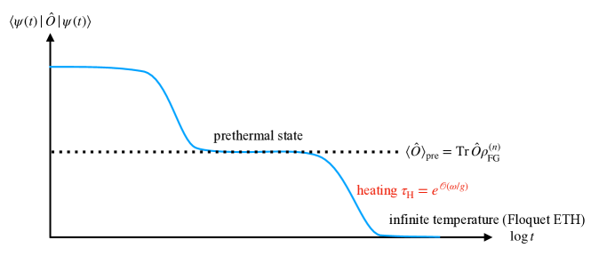
Figure 1: Schematic picture of Floquet prethermalization. The time evolution of $\expectationvalue{\hat{O}}{\psi(t)}$ for a local observable $\hat{O}$ exhibits a two-step relaxation. After the first relaxation, the system reaches a prethermal state described by $\rho_{\mathrm{FG}}^{(n)}$. The second relaxation is due to heating, which occurs in a timescale $\tau_{\mathrm{H}}$, which is large exponentially in $\omega/g$.

The high-frequency expansion is a powerful tool, but we should be careful about its applicability. D’Alessio and Rigol [66] and Lazarides et al. [67] conjectured through exact diagonalization of $\hat{H}_{\mathrm{F}}$ that any eigenstate of $\hat{H}_{\mathrm{F}}$ in a nonintegrable system is locally equivalent to the infinite temperature ensemble for any finite $\omega$ in the thermodynamic limit. This conjecture has been evidenced by numerical calculations for various nonintegrable models [66, 67, 68], and is now called the Floquet eigenstate thermalization hypothesis (ETH) [69] (but also see References [70, 71, 72] for dynamical freezing phenomena). The Floquet ETH implies that $\hat{H}_{\mathrm{F}}$ is a highly nonlocal operator although $\hat{H}_{\mathrm{F}}^{(n)}$ is local for not too large $n$. It means that the exact Floquet Hamiltonian $\hat{H}_{\mathrm{F}}$ and a truncation $\hat{H}_{\mathrm{F}}^{(n)}$ of its high-frequency expansion with a finite $n$ have qualitatively distinct properties. Indeed, the non-locality of $\hat{H}_{\mathrm{F}}$ is understood as the divergence of the high-frequency expansion for any finite $\omega$ in the thermodynamic limit [66, 67]. A rigorous analysis [7] indicates that the divergence begins at an order $n_{0}\propto\omega/g$, which is large in the high-frequency regime. When $n<n_{0}$, the high-frequency expansion looks convergent.

Physically, the Floquet ETH is related to the fact that the system eventually heats up to infinite temperature. The locality of $\hat{H}_{\mathrm{F}}^{(n)}$ implies that a truncation of the high-frequency expansion does not capture the heating process. Heating is a nonperturbative phenomenon in $1/\omega$, and $\hat{H}_{\mathrm{F}}^{(n)}$ may describe the system before heating takes place. Indeed, rigorous analysis of the high-frequency expansion has revealed that heating in quantum [8, 7, 9, 10] and classical [73] spin systems is exponentially slow in frequency, and a system driven by quickly oscillating external fields generically shows two-step relaxation referred to as the Floquet prethermalization [69]. In a timescale much shorter than the heating time $\tau_{\mathrm{H}}=e^{\order{\omega/g}}$, the dynamics is described by $\hat{H}_{\mathrm{F}}^{(n)}$. Therefore, the system will first thermalize under $\hat{H}_{\mathrm{F}}^{(n)}$, and a prethermal state is described by a truncated Floquet-Gibbs state $\rho_{\mathrm{FG}}^{(n)}=e^{-\beta\hat{H}_{\mathrm{F}}^{(n)}}/\Tr e^{-\beta\hat{H}_{\mathrm{F}}^{(n)}}$, where $n$ is arbitrary as long as it is smaller than $n_{0}$. Here, $\beta$ is the inverse temperature of the system at the initial state $\ket{\psi_{\mathrm{ini}}}$, which is determined by $\Tr(\hat{H}_{\mathrm{F}}^{(n)}\rho_{\mathrm{FG}}^{(n)})=\expectationvalue{\hat{H}_{\mathrm{F}}^{(n)}}{\psi_{\mathrm{ini}}}$. In a timescale longer than $\tau_{\mathrm{H}}$, the system will heat up to infinite temperature as predicted by the Floquet ETH for $\hat{H}_{\mathrm{F}}$. See fig. 1 for a schematic picture of the Floquet prethermalization.

The Floquet prethermalization has also been shown to occur in classical systems [74, 75, 76] and boson systems [77, 78], which are not covered by rigorous results. Floquet prethermalization has also been observed in recent experiments [79, 80].

2.4 Floquet Reference Frame

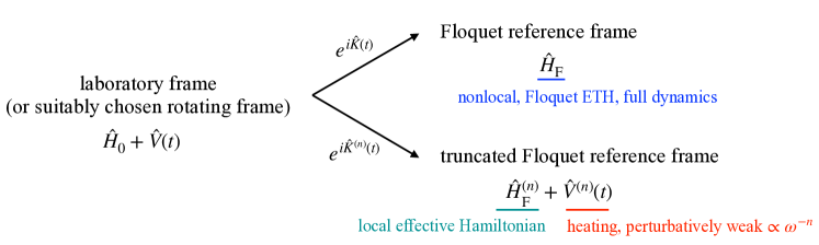
Figure 2: Brief summary of the transformation to the (truncated) Floquet reference frame. In the Floquet reference frame, the Hamiltonian $\hat{H}_{\mathrm{F}}$ becomes completely time-independent, but is highly nonlocal and obeys the Floquet ETH. In the truncated Floquet reference frame, the Hamiltonian consists of an effective static Hamiltonian $\hat{H}_{\mathrm{F}}^{(n)}$ and a perturbatively weak driving field $\hat{V}^{(n)}(t)$.

The decomposition of eq. 2 means that if we move to a special rotating frame via the periodic unitary transformation as $\ket{\psi^{\prime}(t)}=e^{i\hat{K}(t)}\ket{\psi(t)}$, $\hat{H}_{\mathrm{F}}$ plays the role of the Hamiltonian in that rotating frame: $i\differential\ket{\psi^{\prime}(t)}/\differential t=\hat{H}_{\mathrm{F}}\ket{\psi^{\prime}(t)}$. We call this special rotating frame the “Floquet reference frame” to distinguish it from other rotating frames introduced in sections 2.2.1 and 2.2.2. The decomposition of eq. 2 is therefore interpreted as follows: we can always find the Floquet reference frame in which the time dependence of the Hamiltonian is completely washed out.

When we consider a many-body system in which the Floquet ETH holds, $\hat{H}_{\mathrm{F}}$ is too complicated and the Floquet reference frame is not so convenient. Mori [81] introduced a “truncated Floquet reference frame” associated with a periodic unitary transformation $e^{i\hat{K}^{(n)}(t)}$, where $\hat{K}^{(n)}(t)$ is defined by truncating the high-frequency expansion for the micromotion operator:

$$\hat{K}^{(n)}(t)=\sum_{k=1}^{n}\frac{\Lambda_{k}(t)}{\omega^{k}}.$$ (14)

The Hamiltonian in the truncated Floquet reference frame, which is called the “dressed Hamiltonian” reads

$$\tilde{H}^{(n)}(t)=e^{i\hat{K}^{(n)}(t)}\quantity[\hat{H}(t)-i\derivative{t}]e^{-i\hat{K}^{(n)}(t)}\approx\hat{H}_{\mathrm{F}}^{(n)}+\hat{V}^{(n)}(t),$$ (15)

where we ignore terms of $\order{(g/\omega)^{n+1}}$ or higher, and

$$\hat{V}^{(n)}(t)=\frac{1}{\omega^{n+1}}\derivative{\hat{\Lambda}_{n+1}(t)}{t}$$ (16)

is called the dressed driving field satisfying $\hat{V}^{(n)}(t)=\hat{V}^{(n)}(t+T)$ and $\int_{0}^{T}\differential t\,\hat{V}^{(n)}(t)=0$. Remarkably, the truncated Floquet Hamiltonian $\hat{H}_{\mathrm{F}}^{(n)}$ appears as a static part of the dressed Hamiltonian. Unlike the Floquet reference frame, the time-dependence of the Hamiltonian is not completely removed. However, the dressed driving field $\hat{V}^{(n)}(t)$ is effectively weakened ($\hat{V}^{(n)}(t)\propto\omega^{-n}$), and we can treat it perturbatively even if the original driving field $\hat{V}(t)$ is strong [81]. As we argued in section 2.3, $\hat{H}_{\mathrm{F}}^{(n)}$ does not induce heating. The dressed driving field $\hat{V}^{(n)}(t)$ is therefore responsible for heating in the truncated Floquet reference frame.

We summarize the above discussion in fig. 2.

3 FLOQUET MASTER EQUATION FORMALISM

Now we explain how the effect of dissipation is taken into account. A standard setup in considering dissipation is to suppose that the system of interest and the environment (or the bath) constitute a closed system. See fig. 3 for an illustrative picture of the setup. The dynamics of the system of interest is obtained by tracing out the bath degrees of freedom.

Theoretical formulation of open Floquet systems is almost parallel with static open systems [82]. We first perform the Born-Markov approximation for exact equations of motion. Consequently, we obtain a quantum master equation of the Redfield form [83]. By considering an ideal limit (the weak-coupling limit or the singular-coupling limit), we obtain a quantum master equation of the Lindblad form [84, 85].

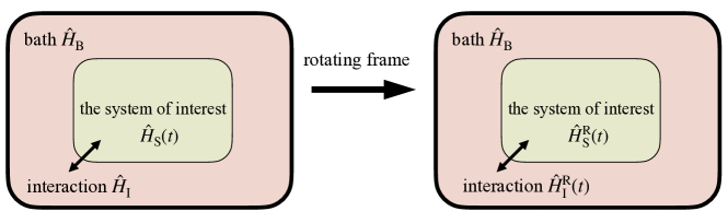
Figure 3: Setup of open Floquet systems. Consider an isolated system consisting of the system of interest (S) and the bath (B) interacting with each other via $\hat{H}_{\mathrm{I}}$. Periodic driving is applied only to the system, and hence only $\hat{H}_{\mathrm{S}}(t)$ depends on time. When periodic driving is strong or resonant, it is often convenient to consider the problem in an appropriate rotating frame, where the interaction Hamiltonian can also periodically depend on time.

3.1 Born-Markov Approximation

Let us denote by $\hat{H}_{\mathrm{S}}(t)$, $\hat{H}_{\mathrm{B}}$, $\hat{H}_{\mathrm{I}}(t)$ the Hamiltonian of the system of interest, that of the bath, and the interaction Hamiltonian, respectively. It is assumed that $\hat{H}_{\mathrm{S}}(t)=\hat{H}_{\mathrm{S}}(t+T)$ and $\hat{H}_{\mathrm{I}}(t)=\hat{H}_{\mathrm{I}}(t+T)$. The Hamiltonian of the total system is given by $\hat{H}_{\mathrm{T}}(t)=\hat{H}_{\mathrm{S}}(t)+\hat{H}_{\mathrm{B}}+\hat{H}_{\mathrm{I}}(t)$. Without loss of generality, we can assume $\Tr_{\mathrm{B}}[\hat{H}_{\mathrm{I}}(t)]=0$.

It is assumed that the periodic driving is applied only to the system of interest, but we allow that the interaction Hamiltonian $\hat{H}_{\mathrm{I}}(t)$ depends on time to consider applications to the Floquet engineering. Indeed, as is explained in sections 2.2.1 and 2.2.2, it is sometimes convenient to move to a suitable rotating frame. The interaction Hamiltonian in a rotating frame generally depends on time, even though it is time-independent in the laboratory frame. Thus, allowing the time dependence of $\hat{H}_{\mathrm{I}}(t)$ enables us to consider the problem in a rotating frame. We also assume that the bath is in thermal equilibrium at the inverse temperature $\beta$, which is expressed by the density matrix $\rho_{\mathrm{B}}=e^{-\beta\hat{H}_{\mathrm{B}}}/Z_{\mathrm{B}}$, where $Z_{\mathrm{B}}$ is the partition function.

The density matrix of the total system $\rho_{\mathrm{T}}$ obeys the Liouville-von Neumann equation:

$$\derivative{t}\rho_{\mathrm{T}}(t)=-i[\hat{H}_{\mathrm{T}}(t),\rho_{\mathrm{T}}(t)]=\quantity(\mathcal{L}_{\mathrm{S}}(t)+\mathcal{L}_{\mathrm{B}}+\mathcal{L}_{\mathrm{I}}(t))\rho_{\mathrm{T}}(t),$$ (17)

where $\mathcal{L}_{\mathrm{X}}(t)=-i[\hat{H}_{\mathrm{X}}(t),\cdot]$ for $\mathrm{X}\in\{\mathrm{S},\mathrm{B},\mathrm{I}\}$. The reduced density matrix is defined as $\rho_{\mathrm{S}}(t)=\Tr_{\mathrm{B}}\rho_{\mathrm{T}}(t)$. We now assume a timescale separation $\tau_{\mathrm{B}}\ll\tau_{\mathrm{R}}$, where $\tau_{\mathrm{B}}$ and $\tau_{\mathrm{R}}$ denote the bath correlation time and the relaxation time due to dissipation. Then, the Born approximation is justified, which yields the following equation of motion for $\rho_{\mathrm{S}}(t)$ [82] starting with an initial time $t_{0}$:

$$\derivative{t}\rho_{\mathrm{S}}(t)=\mathcal{L}_{\mathrm{S}}(t)\rho_{\mathrm{S}}(t)+\int_{0}^{t-t_{0}}\differential s\,\Tr_{\mathrm{B}}\quantity[\mathcal{L}_{\mathrm{I}}(t)\mathcal{L}_{\mathrm{I}}(t,t-s)\rho_{\mathrm{S}}(t)\otimes\rho_{\mathrm{B}}]+\mathcal{I}_{t,t_{0}}[\rho_{\mathrm{T}}(t_{0})],$$ (18)

where $\mathcal{L}_{\mathrm{I}}(t,t-s)=-i[\hat{H}_{\mathrm{I}}(t,t-s),\cdot]$ with $\hat{H}_{\mathrm{I}}(t,t-s)=\mathcal{T}\quantity(e^{\int_{t-s}^{t}\differential t^{\prime}\,[\mathcal{L}_{S}(t^{\prime})+\mathcal{L}_{\mathrm{B}}]})\hat{H}_{\mathrm{I}}(t-s)$ and $\mathcal{I}_{t,t_{0}}[\rho_{\mathrm{T}}(t_{0})]$ stands for the effect of the initial correlation between the system and the bath. Explicitly, $\mathcal{I}_{t,t_{0}}[\rho_{\mathrm{T}}(t_{0})]$ is expressed as, in the leading order of $\tau_{\mathrm{B}}/\tau_{\mathrm{R}}$,

$$\mathcal{I}_{t,t_{0}}[\rho_{\mathrm{T}}(t_{0})]=\Tr_{\mathrm{B}}\mathcal{L}_{\mathrm{I}}(t)\mathcal{T}\quantity[e^{\int_{t_{0}}^{t}\differential t^{\prime}\,[\mathcal{L}_{\mathrm{S}}(t^{\prime})+\mathcal{L}_{\mathrm{B}}]}]\delta\rho_{\mathrm{T}}(t_{0}),$$ (19)

where $\delta\rho_{\mathrm{T}}(t_{0})$ describes the system-bath correlations:

$$\delta\rho_{\mathrm{T}}(t_{0})=\rho_{\mathrm{T}}(t_{0})-\rho_{\mathrm{S}}(t_{0})\otimes\rho_{\mathrm{B}}.$$ (20)

Next, we perform the Markov approximation, which states that we can take the limit of $t-t_{0}\to\infty$ in eq. 18:

$$\int_{0}^{t-t_{0}}\differential s\,\Tr_{\mathrm{B}}\quantity[\mathcal{L}_{\mathrm{I}}(t)\mathcal{L}_{\mathrm{I}}(t,t-s)\rho_{\mathrm{S}}(t)\otimes\rho_{\mathrm{B}}]+\mathcal{I}_{t,t_{0}}[\rho_{\mathrm{T}}(t_{0})]$$

$$\approx\int_{0}^{\infty}\differential s\,\Tr_{\mathrm{B}}\quantity[\mathcal{L}_{\mathrm{I}}(t)\mathcal{L}_{\mathrm{I}}(t,t-s)\rho_{\mathrm{S}}(t)\otimes\rho_{\mathrm{B}}],$$ (21)

which is also justified when $\tau_{\mathrm{B}}/\tau_{\mathrm{R}}\ll 1$ as well as $t-t_{0}\gg\tau_{\mathrm{B}}$ [86].

Now we put $\hat{H}_{\mathrm{I}}(t)=\sum_{i}\hat{X}_{i}(t)\otimes\hat{Y}_{i}$, where $\hat{X}_{i}(t)$ is an operator acting to the system of interest and $\hat{Y}_{i}$ is an operator acting to the bath. Here, the periodicity of $\hat{H}_{\mathrm{I}}(t)$ implies $\hat{X}_{i}(t)=\hat{X}_{i}(t+T)$, and we can always choose $\hat{X}_{i}(t)$ and $\hat{Y}_{i}$ as Hermitian: $\hat{X}_{i}(t)=\hat{X}_{i}(t)^{\dagger}$ and $\hat{Y}_{i}=\hat{Y}_{i}^{\dagger}$ We also define the bath correlation function as $\Phi_{ij}(t)=\Tr_{\mathrm{B}}\quantity[\hat{Y}_{i}(t)\hat{Y}_{j}\rho_{\mathrm{B}}]$ with $\hat{Y}_{i}(t)=e^{i\hat{H}_{\mathrm{B}}t}\hat{Y}_{i}e^{-i\hat{H}_{\mathrm{B}}t}$ ($\tau_{\mathrm{B}}$ corresponds to a characteristic decay time of $\Phi_{ij}(t)$). The Born-Markov quantum master equation is then obtained:

$$\derivative{t}\rho_{\mathrm{S}}(t)=-i\quantity[\hat{H}_{\mathrm{S}}(t),\rho_{\mathrm{S}}(t)]-\sum_{i}\quantity[\hat{X}_{i}(t),\hat{R}_{i}(t)\rho_{\mathrm{S}}(t)-\rho_{\mathrm{S}}(t)\hat{R}_{i}^{\dagger}(t)],$$ (22)

where

$$\hat{R}_{i}(t)=\sum_{j}\int_{0}^{\infty}\differential s\,\hat{X}_{j}(t,t-s)\Phi_{ij}(s),\quad\hat{X}_{j}(t,t-s)=\mathcal{T}e^{\int_{t-s}^{t}\differential t^{\prime}\,\mathcal{L}_{\mathrm{S}}(t^{\prime})}\hat{X}_{j}(t-s).$$ (23)

Equation 22 is called the Floquet-Redfield equation since its right-hand side is known as the Redfield form [83].

It should be emphasized that $\hat{R}_{i}(t)$ depends on $\hat{H}_{\mathrm{S}}(t)$. Consequently, when periodic driving is applied, we cannot use the dissipator derived for an undriven system. The dissipator should be modified by periodic driving. Kohler et al. [87] investigated this effect and concluded that it becomes increasingly important when we consider stronger driving and lower temperatures.

Finally, we make a remark on the Markov approximation. Suppose that eq. 21 is satisfied at a certain time $t$: the time evolution of the system of interest is Markovian at time $t$. Now this $t$ is chosen as a new initial time: we put $t_{0}=t$. Since the time evolution should be independent of our choice of the initial time, eq. 21 must be satisfied at $t_{0}=t$, which yields the following equality:

$$\Tr_{\mathrm{B}}\mathcal{L}_{\mathrm{I}}(t)\delta\rho_{\mathrm{T}}(t)\approx\int_{0}^{\infty}\differential s\,\Tr_{\mathrm{B}}\quantity[\mathcal{L}_{\mathrm{I}}(t)\mathcal{L}_{\mathrm{I}}(t,t-s)\rho_{\mathrm{S}}(t)\otimes\rho_{\mathrm{B}}].$$ (24)

The system-bath correlation $\delta\rho_{\mathrm{T}}(t)$ must satisfy the above nontrivial relation during the Markovian time evolution. Such correlations are called “natural correlations” [88]. For example, the reduced equilibrium state $\rho_{\mathrm{S}}^{\mathrm{eq}}=\Tr_{\mathrm{B}}e^{-\beta\hat{H}_{\mathrm{T}}}/\Tr e^{-\beta\hat{H}_{\mathrm{T}}}$ is shown to satisfy eq. 24 [89]. However, natural correlations do not exist for some $\rho_{\mathrm{S}}$. For example, when the system of interest is in a pure state, the state of the total system must be of the product form, and thus eq. 24 cannot hold. For such an initial state, the time evolution is inevitably non-Markovian at short times $t\lesssim\tau_{\mathrm{B}}$ [90, 91] due to the violation of eq. 24. Then, the initial state of the Redfield equation should be restricted to a subset of density matrices every member of which allows natural correlations with the bath.

Equation 22 is not of the Lindblad form. It is sometimes argued that a “physical” Markovian generator must be of the Lindblad form because otherwise the complete positivity is violated [84, 85]. It should be noted that this argument implicitly assumes that the complete positivity should be imposed to an arbitrary initial state. As we saw above, possible initial states of the Redfield equation are restricted to a certain subset of density matrices. Then, it is not necessary to require the complete positivity for an arbitrary initial state, and hence physical Markovian generator may not be of the Lindblad form. Indeed, it has numerically been demonstrated that the positivity in a Redfield equation holds for suitably restricted initial states [88], although there is no rigorous proof.

3.2 Floquet-Redfield Equation in the Floquet Reference Frame

We rewrite eq. 22 in a useful form. Let us move to the Floquet reference frame:

$$\left\{\begin{aligned} &\tilde{\rho}_{\mathrm{S}}(t)=e^{i\hat{K}(t)}\rho_{\mathrm{S}}(t)e^{-i\hat{K}(t)},\\ &\tilde{X}_{i}(t)=e^{i\hat{K}(t)}\hat{X}_{i}(t)e^{-i\hat{K}(t)}=\sum_{m=-\infty}^{\infty}\tilde{X}_{i,m}e^{im\omega t},\\ &\tilde{R}_{i}(t)=e^{i\hat{K}(t)}\hat{R}_{i}(t)e^{-i\hat{K}(t)}=\sum_{m=-\infty}^{\infty}\tilde{R}_{i,m}e^{im\omega t}.\end{aligned}\right.$$ (25)

By using eqs. 2 and 23, it is shown that $\tilde{R}_{i,m}$ is expressed as follows:

$$\tilde{R}_{i,m}=\sum_{j}\int_{0}^{\infty}\differential s\,e^{-i\hat{H}_{\mathrm{F}}s}\tilde{X}_{j,m}e^{i\hat{H}_{\mathrm{F}}s}e^{-im\omega s}\Phi_{ij}(s).$$ (26)

Equation 22 is then expressed as

$$\derivative{t}\tilde{\rho}_{\mathrm{S}}(t)=-i\quantity[\hat{H}_{\mathrm{F}},\tilde{\rho}_{\mathrm{S}}(t)]-\sum_{i}\sum_{m,l=-\infty}^{\infty}e^{i(m+l)\omega t}\quantity[\tilde{X}_{i,m},\tilde{R}_{i,l}\tilde{\rho}_{\mathrm{S}}(t)-\tilde{\rho}_{\mathrm{S}}(t)\tilde{R}_{i,-l}^{\dagger}].$$ (27)

When $\omega$ is large enough, we may further expect that contributions from $l\neq-m$ in eq. 27 are negligible because of a quickly oscillating factor $e^{i(m+l)\omega t}$. We then have

$$\derivative{t}\tilde{\rho}_{\mathrm{S}}(t)=-i\quantity[\hat{H}_{\mathrm{F}},\tilde{\rho}_{\mathrm{S}}(t)]-\sum_{i}\sum_{m=-\infty}^{\infty}\quantity[\tilde{X}_{i,m},\tilde{R}_{i,-m}\tilde{\rho}_{\mathrm{S}}(t)-\tilde{\rho}_{\mathrm{S}}(t)\tilde{R}_{i,m}^{\dagger}],$$ (28)

which can be used as an approximation of the Floquet-Redfield equation [92, 51].

If we denote by $\tilde{\rho}_{\mathrm{ss}}$ the stationary solution of eq. 28, the density matrix $\rho_{\mathrm{S}}(t)$ in the original frame will relax to a periodic steady state $\rho_{\mathrm{ss}}(t)=e^{-i\hat{K}(t)}\tilde{\rho}_{\mathrm{ss}}e^{i\hat{K}(t)}$ satisfying $\rho_{\mathrm{ss}}(t)=\rho_{\mathrm{ss}}(t+T)$.

We can also write down the Floquet-Redfield equation in a truncated Floquet reference frame. It is obtained by replacing $\hat{H}_{\mathrm{F}}$ by $\hat{H}_{\mathrm{F}}^{(n)}+\hat{V}^{(n)}(t)$ and $\hat{K}(t)$ by $\hat{K}^{(n)}(t)$ in eq. 25.

3.3 Quantum Master Equations of the Lindblad Form

We have derived the Floquet-Redfield equation under the assumption of $\tau_{\mathrm{B}}\ll\tau_{\mathrm{R}}$. In the argument so far, the timescale $\tau_{\mathrm{S}}$ of the intrinsic evolution of the system of interest did not matter. In the following, we derive quantum master equations of the Lindblad form in some limiting cases depending on $\tau_{\mathrm{S}}$. In section 3.3.1, we consider the weak-coupling limit $\tau_{\mathrm{R}}\to\infty$, implying $\tau_{\mathrm{S}}\ll\tau_{\mathrm{R}}$ in addition to $\tau_{\mathrm{B}}\ll\tau_{\mathrm{R}}$. In section 3.3.2, we consider another limit called the singular coupling limit $\tau_{\mathrm{B}}\to 0$, implying $\tau_{\mathrm{B}}\ll\tau_{\mathrm{S}}$ in addition to $\tau_{\mathrm{B}}\ll\tau_{\mathrm{R}}$.

As we will see in section 3.3.1, the weak-coupling limit leads to a Lindblad equation with nonlocal dissipator. It is argued that the weak-coupling approximation cannot describe nontrivial balance of heating and dissipation. On the other hand, the singular-coupling limit leads to a Lindblad equation with local dissipator. However, its steady state is the trivial infinite-temperature ensemble, which is not of great interest in practice. In section 3.3.3 we show that a local Lindblad equation with a non-trivial steady state is obtained under certain conditions by using resonant driving.

3.3.1 Weak Coupling Limit

If we assume $\tau_{\mathrm{S}}\ll\tau_{\mathrm{R}}$ in addition to $\tau_{\mathrm{B}}\ll\tau_{\mathrm{R}}$, eq. 28 is further simplified. This situation is realized in the weak-coupling limit: we consider the scaling $\hat{H}_{\mathrm{T}}(t)=\hat{H}_{\mathrm{S}}(t)+\hat{H}_{\mathrm{B}}+\lambda\hat{H}_{\mathrm{I}}(t)$ and take the limit of $\lambda\to 0$ with $\lambda^{2}t$ held fixed, which is known as the van Hove limit [93]. The scaling parameter $\lambda$ characterizes the strength of dissipation, and $\tau_{\mathrm{R}}\sim\lambda^{-2}$.

In order to investigate the weak-coupling limit, let us consider the problem in the interaction picture: $\tilde{\rho}_{\mathrm{S}}^{\mathrm{(I)}}(t)=e^{-i\hat{H}_{\mathrm{F}}t}\tilde{\rho}_{\mathrm{S}}(t)e^{i\hat{H}_{\mathrm{F}}t}$. The operators $\tilde{X}_{i,m}$ and $\tilde{R}_{i,m}$ in eq. 28 is transformed as

$$\left\{\begin{aligned} &\tilde{X}_{i,m}^{\mathrm{(I)}}(t)=e^{i\hat{H}_{\mathrm{F}}t}\tilde{X}_{i,m}e^{-i\hat{H}_{\mathrm{F}}t}=\sum_{\Omega}\tilde{X}_{i,m}[\Omega]e^{i\Omega t},&&\tilde{X}_{i,m}[\Omega]=\sum_{a,b:\varepsilon_{a}-\varepsilon_{b}=\Omega}\matrixelement{u_{a}}{\tilde{X}_{i,m}}{u_{b}},\\ &\tilde{R}_{i,m}^{\mathrm{(I)}}(t)=e^{i\hat{H}_{\mathrm{F}}t}\tilde{R}_{i,m}e^{-i\hat{H}_{\mathrm{F}}t}=\sum_{\Omega}\tilde{R}_{i,m}[\Omega]e^{i\Omega t},&&\tilde{R}_{i,m}[\Omega]=\sum_{a,b:\varepsilon_{a}-\varepsilon_{b}=\Omega}\matrixelement{u_{a}}{\tilde{R}_{i,m}}{u_{b}},\end{aligned}\right.$$ (29)

where recall that $\{\varepsilon_{a}\}$ are quasi-energies and $\{\ket{u_{a}}\}$ are Floquet eigenstates. By using a rescaled time $\tau=\lambda^{2}t$, eq. 28 is written in the interaction picture as

$$\derivative{\tau}\tilde{\rho}_{\mathrm{S}}^{\mathrm{(I)}}=-\sum_{i}\sum_{m=-\infty}^{\infty}\sum_{\Omega,\Omega^{\prime}}\exp\quantity(i\frac{\Omega+\Omega^{\prime}}{\lambda^{2}}\tau)\quantity[\tilde{X}_{i,m}[\Omega],\tilde{R}_{i,-m}[\Omega^{\prime}]\tilde{\rho}_{\mathrm{S}}^{\mathrm{(I)}}-\tilde{\rho}_{\mathrm{S}}^{\mathrm{(I)}}\tilde{R}_{i,m}[-\Omega^{\prime}]^{\dagger}].$$ (30)

For small $\lambda$, the factor $\exp\quantity(i\frac{\Omega+\Omega^{\prime}}{\lambda^{2}}\tau)$ will rapidly oscillate unless $\Omega^{\prime}=-\Omega$. It is therefore a reasonable approximation that this factor is averaged out in the limit of $\lambda\to 0$. This approximation is called the secular approximation or the rotating-wave approximation in literature [82]. Actually, the secular approximation becomes exact in the van Hove limit under certain conditions [94].

By using eq. 26, we can express $\tilde{R}_{i,m}[\Omega]$ as

$$\tilde{R}_{i,m}[\Omega] =\sum_{j}\tilde{X}_{j,m}[\Omega]\int_{0}^{\infty}\differential s\,\Phi_{ij}(s)e^{-i(\Omega+m\omega)s}$$

$$=\sum_{j}\tilde{X}_{j,m}[\Omega]\quantity[\frac{1}{2}\gamma_{ij}(\Omega+m\omega)+i\eta_{ij}(\Omega+m\omega)],$$ (31)

where $\gamma_{ij}(\varepsilon)$ and $\eta_{ij}(\varepsilon)$ are defined as $\gamma_{ij}(\varepsilon)=\int_{-\infty}^{\infty}\differential t\,\Phi_{ij}(t)e^{-i\omega t}$ and $\eta_{ij}(\varepsilon)=\mathrm{P}\int_{-\infty}^{\infty}\frac{\differential\varepsilon^{\prime}}{2\pi}\frac{\gamma_{ij}(\varepsilon^{\prime})}{\varepsilon^{\prime}-\varepsilon}$. Here, $\mathrm{P}\int$ denotes Cauchy’s principale value integral. By using the Hermiticity of $\{\hat{Y}_{i}\}$, it is shown that $\gamma_{ij}(\varepsilon)$ and $\eta_{ij}(\varepsilon)$ are Hermitian matrices: $\gamma_{ij}(\varepsilon)=\gamma_{ji}(\varepsilon)^{*}$ and $\eta_{ij}(\varepsilon)=\eta_{ji}(\varepsilon)^{*}$. It is also shown that the matrix $\gamma_{ij}(\omega)$ is positive semidefinite. When the bath is in thermal equilibrium at the inverse temperature $\beta$, the Kubo-Martin-Schwinger (KMS) relation holds:

$$\gamma_{ij}(\varepsilon)=\gamma_{ji}(-\varepsilon)e^{-\beta\varepsilon}.$$ (32)

By performing the secular approximation and substituting eq. 31 into eq. 30, we obtain a quantum master equation of the Lindblad form, which is expressed in the Schödinger picture as

$$\derivative{t}\tilde{\rho}_{\mathrm{S}}(t)=-i\quantity[\hat{H}_{\mathrm{F}}+\hat{H}_{\mathrm{LS}},\tilde{\rho}_{\mathrm{S}}]$$

$$+\lambda^{2}\sum_{ij}\sum_{m=-\infty}^{\infty}\sum_{\Omega}\gamma_{ij}(\Omega+m\omega)\quantity(\tilde{X}_{j,m}[\Omega]\tilde{\rho}_{\mathrm{S}}\tilde{X}_{i,m}[\Omega]^{\dagger}-\frac{1}{2}\quantity{\tilde{X}_{i,m}[\Omega]^{\dagger}\tilde{X}_{j,m}[\Omega],\tilde{\rho}_{\mathrm{S}}}),$$ (33)

where $\hat{H}_{\mathrm{LS}}$ is the Lamb-shift Hamiltonian given by

$$\hat{H}_{\mathrm{LS}}=\lambda^{2}\sum_{ij}\sum_{m=-\infty}^{\infty}\sum_{\Omega}\eta_{ij}(\Omega+m\omega)\tilde{X}_{i,m}[\Omega]^{\dagger}\tilde{X}_{j,n}[\Omega].$$ (34)

Equation 33 is called the Floquet-Lindblad equation.

Generally, the dissipator of a Lindblad equation obtained by taking the weak-coupling limit is nonlocal even in the absence of driving field [94]. This nonlocality can be physically interpreted in the following way: a local excitation of the system will spread over the entire system until it dissipates into the bath.

It should be emphasized that the validity of the Floquet-Lindblad equation is severely limited due to the nature of the secular approximation. We have assumed $\tau_{\mathrm{R}}\gg\tau_{\mathrm{S}}$ for any relevant timescale $\tau_{\mathrm{S}}$ of the system of interest. In macroscopic open Floquet systems, however, we are typically interested in the situation in which this assumption does not hold. When the system is driven by periodic fields, heating is obviously an important process, and hence its timescale $\tau_{\mathrm{H}}$ enters into $\tau_{\mathrm{S}}$. We expect that some nontrivial (periodic) stationary state is realized by a balance between dissipation and heating. Such a balance requires $\tau_{\mathrm{R}}\lesssim\tau_{\mathrm{H}}$, but it contradicts the weak-coupling limit $\tau_{\mathrm{R}}\to\infty$. In other words, the weak-coupling limit implicitly assumes that heating is always faster than dissipation, and hence any nontrivial balance of heating and dissipation cannot be described by the weak-coupling Floquet-Lindblad equation.

3.3.2 Singular Coupling Limit

We consider another limiting procedure: $\tau_{\mathrm{B}}\ll\tau_{\mathrm{S}}$ and $\tau_{\mathrm{B}}\ll\tau_{\mathrm{R}}$. This situation is dealt with the scaling $\hat{H}_{\mathrm{T}}(t)=\hat{H}_{\mathrm{S}}(t)+\lambda^{-2}\hat{H}_{\mathrm{B}}+\lambda^{-1}\hat{H}_{\mathrm{I}}(t)$ and $\beta=\lambda^{2}\tilde{\beta}$ ($\tilde{\beta}$ is independent of $\lambda$). We take the limit of $\lambda\to 0$ with this scaling, which is called the singular coupling limit. The bath correlation function is written as

$$\Phi_{ij}(t)=\Tr_{\mathrm{B}}\quantity[e^{i\hat{H}_{\mathrm{B}}t/\lambda^{2}}\hat{Y}_{i}e^{-i\hat{H}_{\mathrm{B}}t/\lambda^{2}}\hat{Y}_{j}\frac{e^{-\tilde{\beta}\hat{H}_{\mathrm{B}}}}{\Tr_{\mathrm{B}}e^{-\tilde{\beta}\hat{H}_{\mathrm{B}}}}]\eqqcolon\tilde{\Phi}_{ij}\quantity(\frac{t}{\lambda^{2}}).$$ (35)

In the limit of $\lambda\to 0$, $\Phi_{ij}(t)$ becomes a delta function. The operator $\hat{R}_{i}(t)$ in eq. 23 is therefore simplified as

$$\hat{R}_{i}(t)\approx\lambda^{2}\sum_{j}\hat{X}_{j}\int_{0}^{\infty}\differential\tau\,\tilde{\Phi}_{ij}(\tau)\eqqcolon\lambda^{2}\sum_{j}\hat{X}_{j}\quantity(\frac{1}{2}\gamma_{ij}+i\eta_{ij}),$$ (36)

where $\gamma_{ij}=\gamma_{ji}\geq 0$ and $\eta_{ij}=\eta_{ji}^{*}$ are satisfied. Equation 22 then becomes

$$\derivative{t}\rho_{\mathrm{S}}(t)=-i\quantity[\hat{H}_{\mathrm{S}}(t)+\sum_{ij}\eta_{ij}\hat{X}_{i}\hat{X}_{j},\rho_{\mathrm{S}}(t)]+\sum_{ij}\gamma_{ij}\quantity(\hat{X}_{j}\rho_{\mathrm{S}}(t)\hat{X}_{i}-\frac{1}{2}\quantity{\hat{X}_{i}\hat{X}_{j},\rho_{\mathrm{S}}(t)}).$$ (37)

This is a quantum master equation of the Lindblad form. The dissipator is local in contrast to the Lindblad equation in the weak-coupling limit: any local excitation will immediately dissipate into the bath before it spreads over the system.

Equation 37 has the trivial infinite-temperature ensemble as a steady state. Therefore, the singular-coupling limit cannot describe any nontrivial steady state, unless there are other nontrivial steady states due to some conserved quantities [95].

3.3.3 Phenomenological Lindblad Equation Using Resonant Driving

In the weak-coupling limit, the system is described by the Floquet-Lindblad equation with quite complicated highly nonlocal dissipator. In the study of open quantum systems [96, 97, 98], we sometimes consider a more intuitive “phenomenological” Lindblad equation with dissipator

$$\mathcal{D}(\rho)=\sum_{i}\quantity(\hat{L}_{i}\rho_{\mathrm{S}}\hat{L}_{i}^{\dagger}-\frac{1}{2}\quantity{\hat{L}_{i}^{\dagger}\hat{L}_{i},\rho_{\mathrm{S}}}),$$ (38)

where Lindblad jump operators $\quantity{\hat{L}_{i}}$ are phenomenologically introduced local operators, which may be non-Hermitian in contrast to those in the singular-coupling limit. For example, in a two-level atom described by the Pauli matrices $\quantity{\hat{\sigma}^{x},\hat{\sigma}^{y},\hat{\sigma}^{z}}$ in contact with a photon bath, an excitation of the atom by absorbing a photon is described by a Lindblad jump operator $\hat{L}=\hat{\sigma}^{+}=\quantity(\hat{\sigma}^{x}+i\hat{\sigma}^{y})/2$, whereas a de-excitation by emitting a photon is described by $\hat{L}=\hat{\sigma}^{-}=\quantity(\hat{\sigma}^{x}-i\hat{\sigma}^{y})/2$. In a Bose or Fermi particle described by the creation and annihilation operators $\hat{a}^{\dagger}$ and $\hat{a}$, respectively, the particle loss is described by a Lindblad jump operator $\hat{L}=\hat{a}$ and the dephasing is described by $\hat{L}=\hat{a}^{\dagger}\hat{a}$.

In this section, we present another route to the Lindblad equation from eq. 28, and demonstrate that a certain kind of “phenomenological” Lindblad equations is microscopically derived.

By using eq. 29, we have $e^{-i\hat{H}_{\mathrm{F}}s}\tilde{X}_{j,m}e^{i\hat{H}_{\mathrm{F}}s}=\sum_{\Omega}\tilde{X}_{j,m}[\Omega]e^{-i\Omega s}$. Let us substitute this expression into eq. 26. We then have

$$\tilde{R}_{i,m} =\sum_{j}\sum_{\Omega}\tilde{X}_{j,m}[\Omega]\int_{0}^{\infty}\differential s\,e^{-i(\Omega+m\omega)s}\Phi_{ij}(s)$$

$$=\sum_{j}\sum_{\Omega}\tilde{X}_{j,m}[\Omega]\quantity(\frac{1}{2}\gamma_{ij}(\Omega+m\omega)+i\eta_{ij}(\Omega+m\omega)).$$ (39)

Now let us assume that contributions from $\absolutevalue{\Omega}\ll\omega$ are dominant. Since $\Omega$ typically satisfies $\absolutevalue{\Omega}\lesssim g$, where recall that $g$ denotes a characteristic local energy of $\hat{H}_{\mathrm{S}}(t)$, this assumption will be justified as long as $g\ll\omega$. Under this assumption, we further perform the following approximations in eq. 39:

$$\gamma_{ij}(\Omega+m\omega)\approx\gamma_{ij}(m\omega)\mbox{\quad and\quad}\eta_{ij}(\Omega+m\omega)\approx\eta_{ij}(m\omega).$$ (40)

It should be noted that eq. 40 is justified for $m=0$ only when the temperature of the bath is high enough or $\tilde{X}_{j,0}\approx 0$ in eq. 39. Indeed, the KMS relation $\gamma_{ij}(\varepsilon)=\gamma_{ji}(-\varepsilon)e^{-\beta\varepsilon}$ implies that $\gamma_{ij}(\Omega)$ can be approximated by a constant value only when $\beta\absolutevalue{\Omega}\ll 1$. Therefore, behind eq. 40, it is implicitly assumed that

$$\beta g\ll 1\mbox{\quad or\quad}\tilde{X}_{j,0}\approx 0.$$ (41)

By using eq. 40, we have

$$\tilde{R}_{i,m}\approx\sum_{j}\sum_{\Omega}\tilde{X}_{j,m}[\Omega]\quantity(\frac{1}{2}\gamma_{ij}(m\omega)+i\eta_{ij}(m\omega))=\sum_{j}\tilde{X}_{j,m}\quantity(\frac{1}{2}\gamma_{ij}(m\omega)+i\eta_{ij}(m\omega)).$$ (42)

Substituting it into eq. 28, we obtain

$$\derivative{t}\tilde{\rho}_{\mathrm{S}}(t)= -i\quantity[\hat{H}_{\mathrm{F}}+\hat{H}_{\mathrm{LS}},\tilde{\rho}_{\mathrm{S}}(t)]$$

$$+\sum_{ij}\sum_{m=-\infty}^{\infty}\gamma_{ij}(m\omega)\quantity(\tilde{X}_{j,m}\tilde{\rho}_{\mathrm{S}}(t)\tilde{X}_{i,m}^{\dagger}-\frac{1}{2}\quantity{\tilde{X}_{i,m}^{\dagger}\tilde{X}_{j,m},\tilde{\rho}_{\mathrm{S}}(t)}),$$ (43)

where the Lamb-shift Hamiltonian is given by $\hat{H}_{\mathrm{LS}}=\sum_{ij}\sum_{m=-\infty}^{\infty}\eta_{ij}(m\omega)\tilde{X}_{i,m}^{\dagger}\tilde{X}_{j,m}$. Equation 43 is of the Lindblad form, which has a nontrivial steady state when $\beta\omega=\order{1}$.

We now present a simple example, which leads to a phenomenological Lindblad equation [37]. Let us consider a spin chain driven by circularly polarized fields

$$\hat{H}_{\mathrm{S}}(t)=\sum_{i=1}^{N}\quantity[\frac{\omega+\Delta}{2}\hat{\sigma}_{i}^{z}-J\hat{\sigma}_{i}^{z}\hat{\sigma}_{i+1}^{z}-h\quantity(e^{-i\omega t}\hat{\sigma}_{i}^{+}+e^{i\omega t}\hat{\sigma}_{i}^{-})],$$ (44)

which is in contact with a free-boson bath independently at each site:

$$\hat{H}_{\mathrm{B}}=\sum_{i=1}^{N}\sum_{k}\omega_{k}\hat{b}_{i,k}^{\dagger}\hat{b}_{i,k}\mbox{\quad and\quad}\hat{H}_{\mathrm{I}}=\sum_{i=1}^{N}\hat{\sigma}_{i}^{x}\sum_{k}\lambda_{k}\quantity(\hat{b}_{i,k}+\hat{b}_{i,k}^{\dagger}),$$ (45)

where $\omega_{k}>0$ and $\lambda_{k}\in\mathbb{R}$. The creation and annihilation operators of bosons of the mode $k$ in the $i$th bath are denoted by $b_{i,k}^{\dagger}$ and $b_{i,k}$, respectively. This model is regarded as an example of the systems treated in 2.2.2: $\sum_{i=1}^{N}\hat{\sigma}_{i}^{z}/2$ corresponds to $\hat{N}$ in eq. 13.

We shall move to a rotating frame via the unitary transformation $e^{-i(\omega/2)\sum_{i=1}^{N}\hat{\sigma}_{i}^{z}t}$. The Hamiltonian in the rotating frame is given by

$$\hat{H}_{\mathrm{S}}^{\mathrm{R}}=\sum_{i=1}^{N}\quantity(\frac{\Delta}{2}\hat{\sigma}_{i}^{z}-J\hat{\sigma}_{i}^{z}\hat{\sigma}_{i+1}^{z}-h\hat{\sigma}_{i}^{x}),\quad\hat{H}_{\mathrm{B}}^{\mathrm{R}}=\hat{H}_{\mathrm{B}},\quad\hat{H}_{\mathrm{I}}^{\mathrm{R}}(t)=\sum_{i=1}^{N}\hat{X}_{i}(t)\otimes\hat{Y}_{i},$$ (46)

where $\hat{X}_{i}(t)=\hat{\sigma}_{i}^{+}e^{i\omega t}+\hat{\sigma}_{i}^{-}e^{-i\omega t}$ and $\hat{Y}_{i}=\sum_{k}\lambda_{k}\quantity(\hat{b}_{i,k}+\hat{b}_{i,k}^{\dagger})$. In this model, $\hat{H}_{\mathrm{S}}^{\mathrm{R}}$ does not depend on time, and hence there is no micromotion: $\hat{K}(t)=0$ and we can simply put $\hat{H}_{\mathrm{F}}=\hat{H}_{\mathrm{S}}^{\mathrm{R}}$, $\tilde{X}_{i,1}=\hat{\sigma}_{i}^{+}$, and $\tilde{X}_{i,-1}=\hat{\sigma}_{i}^{-}$. For $m\neq\pm 1$, $\tilde{X}_{i,m}=0$.

Equation 43 is then written as

$$\derivative{t}\rho_{\mathrm{S}}^{\mathrm{R}}(t)=-i\quantity[\hat{H}_{\mathrm{S}}^{\mathrm{R}}+\hat{H}_{\mathrm{LS}},\rho_{\mathrm{S}}^{\mathrm{R}}(t)] +\sum_{i=1}^{N}\gamma(\omega)\quantity(\hat{\sigma}_{i}^{+}\rho_{\mathrm{S}}^{\mathrm{R}}(t)\hat{\sigma}_{i}^{-}-\frac{1}{2}\quantity{\hat{\sigma}_{i}^{-}\hat{\sigma}_{i}^{+},\rho_{\mathrm{S}}^{\mathrm{R}}(t)})$$

$$+\sum_{i=1}^{N}\gamma(-\omega)\quantity(\hat{\sigma}_{i}^{-}\rho_{\mathrm{S}}^{\mathrm{R}}(t)\hat{\sigma}_{i}^{+}-\frac{1}{2}\quantity{\hat{\sigma}_{i}^{+}\hat{\sigma}_{i}^{-},\rho_{\mathrm{S}}^{\mathrm{R}}(t)}).$$ (47)

Here, $\gamma(\varepsilon)$ is calculated as $\gamma(\varepsilon)=\pi\mathrm{sgn}(\varepsilon)J(\absolutevalue{\varepsilon})/(e^{\beta\varepsilon}-1)$, where the bath spectral density $J(\varepsilon)$ is defined as $J(\varepsilon)=\sum_{k}\delta(\omega_{k}-\varepsilon)\lambda_{k}^{2}$.

In eq. 47, the Lindblad jump operators $\quantity{\hat{\sigma}_{i}^{\pm}}$ are very simple and intuitive: they represent an excitation and a de-excitation of a two-level atom via the coupling to the bath. Moreover, the KMS relation $\gamma(\omega)=\gamma(-\omega)e^{-\beta\omega}$ implies that eq. 47 has a nontrivial steady state when $\beta\omega=\order{1}$.

4 STATISTICAL MECHANICS OF FLOQUET SYSTEMS

When an undriven system is in a weak contact with a thermal bath at the inverse temperature $\beta$, equilibrium statistical mechanics predicts that the steady state is described by a Gibbs state $e^{-\beta\hat{H}_{\mathrm{S}}}/\Tr_{\mathrm{S}}e^{-\beta\hat{H}_{\mathrm{S}}}$. A natural question is to what extent the method of equilibrium statistical mechanics is extended to Floquet systems. Since the Floquet theorem offers a static description of the long-time behavior of a closed Floquet system via the Floquet Hamiltonian $\hat{H}_{\mathrm{F}}$ or its approximation $\hat{H}_{\mathrm{F}}^{(n)}$, it is natural to consider a Floquet-Gibbs state $\rho_{\mathrm{FG}}=e^{-\beta\hat{H}_{\mathrm{F}}}/\Tr_{\mathrm{S}}e^{-\beta\hat{H}_{\mathrm{F}}}$ or a truncated Floquet-Gibbs state $\rho_{\mathrm{FG}}^{(n)}=e^{-\beta\hat{H}_{\mathrm{F}}^{(n)}}/\Tr_{\mathrm{S}}e^{-\beta\hat{H}_{\mathrm{F}}^{(n)}}$ as a candidate of the steady state in an open system.

We remark that there is an arbitrariness in the definition of $\rho_{\mathrm{FG}}$ due to the indefiniteness of quasi-energies $\quantity{\varepsilon_{a}}$. In the following discussion, we choose $\varepsilon_{a}$ so that it is closest to the mean energy $\bar{E}_{a}=(1/T)\int_{0}^{T}\differential t\expectationvalue{\hat{H}(t)}{u_{a}(t)}$. On the other hand, there is no arbitrariness in the definition of a truncated Floquet-Gibbs state since the high-frequency expansion naturally fixes the quasi-energies.

The possibility of extending equilibrium statistical mechanics to Floquet systems has been investigated in various previous works. Breuer and Holthaus [48] showed that a periodic steady state of the Floquet-Lindblad equation for a driven harmonic oscillator is given by the Floquet-Gibbs state. On the other hand, Breuer et al. [49] showed that, for a periodically driven particle in a box, the population over Floquet states is significantly distinct from the Boltzmann-Gibbs distribution. Ketzmerick and Wustmann [52] made a similar observation in a driven unharmonic oscillator. In this way, the validity of equilibrium statistical mechanics depends on the specific model Hamiltonian, and hence general considerations have been desirable. Breuer et al. [49] and Kohn [50] pointed out that a transition between two Floquet states with the quasi-energy difference $\Delta\varepsilon$ will be accompanied by bath transitions with many different energy changes $\Delta E=-\Delta\varepsilon+m\omega$ with $m$ being an arbitrary integer, which results in the violation of the detailed-balance condition. Thus, in general, the steady state will be distinct from the Floquet-Gibbs state.

In this section, based on the formalism developed in section 3, we review recent studies [54, 53, 55] investigating general conditions for the validity of equilibrium statistical mechanics to open Floquet systems. In section 4.1, we investigate the steady state of the Floquet-Lindblad equation in the weak-coupling limit. In section 4.2, we investigate the steady state of the Floquet-Redfield equation at a finite system-bath coupling.

4.1 Steady States in the Weak-Coupling Limit

We investigate the steady state of the Floquet-Lindblad equation in the weak-coupling limit given by eq. 33. For simplicity, we assume that $\hat{H}_{\mathrm{F}}$ has no degeneracy. We then find that the dynamics of the diagonal matrix elements $P_{a}(t)=\expectationvalue{\tilde{\rho}_{\mathrm{S}}(t)}{u_{a}}$ in the basis diagonalizing $\hat{H}_{\mathrm{F}}$ is decoupled from that of the off-diagonal matrix elements. The time evolution of $P_{a}(t)$ obeys the following Pauli master equation:

$$\derivative{t}P_{a}(t)=\sum_{b}\quantity(W_{ab}P_{b}(t)-W_{ba}P_{a}(t)),$$ (48)

where $W_{ab}$ stands for the transition rate from the state $\ket{u_{b}}$ to the state $\ket{u_{a}}$, and is explicitly given by

$$W_{ab}=\sum_{ij}\sum_{m=-\infty}^{\infty}\gamma_{ij}(\varepsilon_{a}-\varepsilon_{b}+m\omega)\matrixelement{u_{a}}{\tilde{X}_{j,m}}{u_{b}}\matrixelement{u_{a}}{\tilde{X}_{i,m}}{u_{b}}^{*}$$ (49)

for $a\neq b$, and $W_{aa}=0$ for any $a$.

Without any special reason, every off-diagonal matrix element exponentially decays to zero. Therefore, the steady state $\tilde{\rho}_{\mathrm{ss}}$ is written in the diagonal form $\tilde{\rho}_{\mathrm{ss}}=\sum_{a}P_{a}^{\mathrm{ss}}\outerproduct{u_{a}}{u_{a}}$, where $\quantity{P_{a}^{\mathrm{ss}}}$ is the steady solution of eq. 48 satisfying $\sum_{b}\quantity(W_{ab}P_{b}^{\mathrm{ss}}-W_{ba}P_{a}^{\mathrm{ss}})=0$.

When no driving field is applied, there is no summation over $m$ in eq. 49. In this case, the KMS relation yields the detailed balance condition:

$$W_{ab}e^{-\beta E_{b}}=W_{ba}e^{-\beta E_{a}},$$ (50)

where $\quantity{E_{a}}$ are eigenvalues of $\hat{H}_{\mathrm{S}}$ without driving field. The detailed balance condition ensures that the steady state is given by the Gibbs distribution $P_{a}^{\mathrm{ss}}=e^{-\beta E_{a}}/\sum_{b}e^{-\beta E_{b}}$.

On the other hand, under periodic driving, the system can undergo a transition between Floquet eigenstates by absorbing or emitting $m$ energy quanta. This is the physical meaning of the additional sum over $m$ in eq. 49. Importantly, the sum over $m$ in eq. 49 in general breaks the detailed balance [49, 50], and the steady state is not necessarily given by the Floquet-Gibbs state.

Here, we find the following important observation. Even when the system is subject to periodic driving, the detailed balance condition is approximately satisfied if only $m=0$ is dominant in eq. 49 for any $a$ and $b$. Shirai et al. [54] and Liu [53] investigated the condition for it to happen, which we now explain below.

We first assume that

$$\frac{1}{T}\int_{0}^{T}\differential t\,\norm{\hat{H}_{\mathrm{S}}(t)}\ll\omega.$$ (51)

In this case, the convergence of the high-frequency expansion is guaranteed. It should be noted that if we consider strong driving (section 2.2.1) or resonant driving (section 2.2.2), we must move to the rotating frame so that eq. 51 is satisfied. Under eq. 51, the mean energy $\bar{E}_{a}$ for any Floquet eigenstate satisfies $\absolutevalue{\bar{E}_{a}}\ll\omega$, which implies $\absolutevalue{\varepsilon_{a}}\ll\omega$ in our choice of the quasi-energies. Moreover, the micromotion operator $\hat{K}(t)$ is almost zero: $\hat{K}(t)=\order{\omega^{-1}}$. Thus, $\tilde{X}_{i}(t)\approx\hat{X}_{i}(t)$, and hence $\tilde{X}_{i,m}$ is approximately given by

$$\tilde{X}_{i,m}\approx\frac{1}{T}\int_{0}^{T}\differential t\,\hat{X}_{i}(t)e^{-im\omega t}.$$ (52)

When eq. 51 is satisfied in the laboratory frame, we do not have to move to the rotating frame. In this case, $\hat{X}_{i}$ does not depend on $t$, and hence $\tilde{X}_{i,m}\approx\delta_{m,0}\hat{X}_{i}$. Thus, $m=0$ is dominant in eq. 49 for any $a$ and $b$, which ensures that the Floquet-Gibbs state is realized as a steady state. On the other hand, for strong driving or resonant driving, we must move to the rotating frame to guarantee eq. 51, and the interaction Hamiltonian $\hat{H}_{\mathrm{I}}^{\mathrm{R}}(t)$ can depend on $t$. In this case, there are two situations where $m=0$ is dominant for any $a$ and $b$ in eq. 49: either $\tilde{X}_{i,m}\approx 0$ for all $m\neq 0$ or $\gamma_{ij}(\varepsilon_{a}-\varepsilon_{b}+m\omega)\approx 0$ for all $m\neq 0$. In addition, we have to assume that $(1/T)\int_{0}^{T}\differential t\,\hat{H}_{\mathrm{I}}(t)\approx\sum_{i}\tilde{X}_{i,0}\otimes\hat{Y}_{i}$ does not vanish. Otherwise, we cannot say that the term of $m=0$ is dominant.

First, we consider the possibility of $\tilde{X}_{i,m}\approx 0$ for all $m\neq 0$. This condition is satisfied when the interaction Hamiltonian does not depend on $t$ even in the rotating frame: $\tilde{X}_{i}(t)=\hat{X}_{i}$, and hence eq. 52 leads to $\tilde{X}_{i,m}\approx\delta_{m,0}\hat{X}_{i}$. Under strong driving $\hat{H}_{\mathrm{S}}(t)=\hat{H}_{0}+\omega f(\omega t)\hat{V}$, the interaction Hamiltonian in the rotating frame is given by $\hat{H}_{\mathrm{I}}^{\mathrm{R}}(t)=e^{iF(\omega t)\hat{V}}\hat{H}_{\mathrm{I}}e^{-iF(\omega t)\hat{V}}$, where $F(\theta)=\int_{0}^{\theta}\differential s\,f(\theta)$. We see that it is independent of time when $\hat{H}_{\mathrm{I}}$ commutes with $\hat{V}$. This situation is realized when the periodic field is only applied to a part of the system which is not directly coupled to the bath [54]. Similarly, under resonant driving $\hat{H}_{\mathrm{S}}(t)=\hat{H}_{0}+\omega\hat{N}+\hat{V}(t)$, the interaction Hamiltonian does not depend on $t$ when $\hat{H}_{\mathrm{I}}$ commutes with $\hat{N}$.

Next, we consider the possibility of $\gamma_{ij}(\varepsilon_{a}-\varepsilon_{b}+m\omega)\approx 0$ for all $m\neq 0$. Because of eq. 51, $\absolutevalue{\varepsilon_{a}-\varepsilon_{b}}\ll\omega$, and hence $\varepsilon_{a}-\varepsilon_{b}+m\omega\approx m\omega$. Generally, $\gamma_{ij}(\varepsilon)$ decays for $\varepsilon$ greater than a cutoff frequency $\omega_{c}$, which corresponds to a characteristic local energy scale of the bath. If $\omega\gg\omega_{c}$, which physically means that periodic driving is much faster than the motion of the bath, $\gamma_{ij}(\varepsilon_{a}-\varepsilon_{b}+m\omega)\approx 0$ for all $m\neq 0$ is satisfied because $\absolutevalue{\varepsilon_{a}-\varepsilon_{b}+m\omega}\gg\omega_{c}$.

Let us summarize the condition for the realization of the Floquet-Gibbs state:

(i)

$(1/T)\int_{0}^{T}\differential t\,\norm{\hat{H}_{\mathrm{S}}(t)}\ll\omega$.

(ii)

Either $\quantity[\hat{H}_{\mathrm{I}},\hat{A}]=0$ or $\omega_{c}\ll\omega$. Here, $\hat{A}=\hat{V}$ in the case of strong driving (eq. 8) and $\hat{A}=\hat{N}$ in the case of resonant driving (eq. 13).

(iii)

$(1/T)\int_{0}^{T}\differential t\,\hat{H}_{\mathrm{I}}(t)$ is not vanishingly small.

The condition (i) ensures that the system does not suffer from heating. However, even when (i) is satisfied, periodic driving may indirectly induce excitations in the bath. The conditions (ii) and (iii) ensure that this effect is negligible [99].

4.2 Steady States at Finite System-Bath Coupling

In macroscopic systems, the condition (i) cannot be satisfied, and the system heats up due to periodic driving. In a closed system, a truncated Floquet-Gibbs state $\rho_{\mathrm{FG}}^{(n)}$ is realized only in a prethermal regime. In an open system, on the other hand, it is hopefully expected that dissipation suppresses heating and stabilizes the truncated Floquet-Gibbs state.

Shirai et al. [55] investigated the conditions under which the above scenario is realized. To stabilize the truncated Floquet-Gibbs state, we must consider a finite system-bath coupling, where the Floquet-Lindblad equation is not appropriate. We assume that the Born-Markov approximation is still valid, i.e. $\tau_{\mathrm{B}}\ll\tau_{\mathrm{R}}$. In this case, the dynamics is described by the Floquet-Redfield equation.

Since we want to consider the stability of the truncated Floquet-Gibbs state, it is convenient to employ a truncated Floquet reference frame introduced in section 2.4. The Floquet-Redfield equation in the truncated Floquet reference frame is given by

$$\derivative{t}\tilde{\rho}_{\mathrm{S}}^{(n)}=-i\quantity[\hat{H}_{\mathrm{F}}^{(n)}+\hat{V}^{(n)}(t),\tilde{\rho}_{\mathrm{S}}^{(n)}]-\sum_{i}\sum_{m=-\infty}^{\infty}\quantity[\tilde{X}_{i,m}^{(n)},\tilde{R}_{i,-m}^{(n)}\tilde{\rho}_{\mathrm{S}}^{(n)}-\tilde{\rho}_{\mathrm{S}}^{(n)}\tilde{R}_{i,m}^{(n)\dagger}],$$ (53)

where $\quantity{\tilde{\rho}_{\mathrm{S}}^{(n)}(t),\tilde{X}_{i,m}^{(n)},\tilde{R}_{i,m}^{(n)}}$ are given by replacing $\hat{K}(t)$ by $\hat{K}^{(n)}(t)$ in eq. 25. Let us denote by $\tau_{\mathrm{H}}$ the heating time when the system is isolated from the bath. If $\tau_{\mathrm{R}}\ll\tau_{\mathrm{H}}$ is satisfied, the energy absorbed from the periodic driving field immediately dissipates into the bath and heating is suppressed. In this case, we can drop the term $-i\quantity[\hat{V}^{(n)}(t),\tilde{\rho}_{\mathrm{S}}^{(n)}(t)]$ in eq. 53, and in the same approximation,

$$\tilde{R}_{i,m}^{(n)}\approx\sum_{j}\int_{0}^{\infty}\differential s\,e^{-i\hat{H}_{\mathrm{F}}^{(n)}s}\tilde{X}_{j,m}^{(n)}e^{i\hat{H}_{\mathrm{F}}^{(n)}s}e^{-im\omega s}\Phi_{ij}(s).$$ (54)

After dropping $\hat{V}^{(n)}(t)$ in eq. 53, the steady state $\tilde{\rho}_{\mathrm{ss}}$ satisfies

$$-i\quantity[\hat{H}_{\mathrm{F}}^{(n)},\tilde{\rho}_{\mathrm{ss}}]+\mathcal{D}^{(n)}\quantity[\tilde{\rho}_{\mathrm{ss}}]=0,$$ (55)

where dissipator $\mathcal{D}^{(n)}[\cdot]$ is defined as the last term of eq. 53. We now assume $g^{-1}\ll\tau_{\mathrm{R}}$: dissipation is much weaker than a characteristic local energy scale. We then expect that we can perform the perturbative expansion of $\tilde{\rho}_{\mathrm{ss}}$ in terms of dissipation strength [100]: $\tilde{\rho}_{\mathrm{ss}}=\sum_{l=0}^{\infty}\rho_{l}$, where

$$-i\quantity[\hat{H}_{\mathrm{F}}^{(n)},\rho_{0}]=0,$$ (56)

$$-i\quantity[\hat{H}_{\mathrm{F}}^{(n)},\rho_{l+1}]+\mathcal{D}^{(n)}\quantity[\rho_{l}]=0\mbox{\quad for $l=1,2,\dots$.\quad}$$ (57)

In the following, we put $\tilde{\rho}_{\mathrm{ss}}\approx\rho_{0}$. From eq. 56, we find that $\rho_{0}$ is diagonal in the basis diagonalizing $\hat{H}_{\mathrm{F}}^{(n)}$: $\rho_{0}=\sum_{a}P_{a}\outerproduct*{u_{a}^{(n)}}{u_{a}^{(n)}}$. From eq. 57 with $l=0$, we find $\expectationvalue*{\mathcal{D}^{(n)}[\rho_{0}]}{u_{a}^{(n)}}=0$, which yields

$$\sum_{b}\quantity(W_{ab}^{(n)}P_{b}-W_{ba}^{(n)}P_{a})=0,$$ (58)

where the transition rate $W_{ab}^{(n)}$ is given by

$$W_{ab}^{(n)}=\sum_{ij}\sum_{m=-\infty}^{\infty}\gamma_{ij}(E_{a}^{(n)}-E_{b}^{(n)}+m\omega)\matrixelement{u_{a}^{(n)}}{\tilde{X}_{j,m}^{(n)}}{u_{b}^{(n)}}\matrixelement{u_{a}^{(n)}}{\tilde{X}_{i,m}^{(n)}}{u_{b}^{(n)}}^{*}.$$ (59)

Equation 58 shows that $\quantity{P_{a}}$ is nothing but the steady solution of the Pauli master equation under the transition rates $\quantity{W_{ab}^{(n)}}$. Thus, the truncated Floquet-Gibbs state is realized if the transition rates satisfy the detailed balance condition.

We can repeat the same argument as in section 4.1: The detailed balance condition is satisfied if the sum over $m$ in eq. 59 is dominated by $m=0$ for all $a$ and $b$. Since the high-frequency expansion is divergent, $\hat{H}_{\mathrm{F}}$ and $\hat{K}(t)$ are highly nonlocal operators. On the other hand, the truncated ones $\hat{H}_{\mathrm{F}}^{(n)}$ and $\hat{K}^{(n)}(t)$ are local when $n<n_{c}\sim\omega/g$, which plays an essential role in the following analysis. First, we assume that $\quantity{\hat{X}_{i}(t)}$ are local. Since $\hat{K}^{(n)}(t)=\order{\omega^{-1}}\approx 0$ for large $\omega$, $\tilde{X}_{i,m}^{(n)}\approx(1/T)\int_{0}^{T}\differential t\,\hat{X}_{i}(t)e^{-im\omega t}$, which is also a local operator. In general, if both $\tilde{X}_{i,m}^{(n)}$ and $\hat{H}_{\mathrm{F}}^{(n)}$ are local, matrix elements $\matrixelement*{u_{a}^{(n)}}{\tilde{X}_{i,m}^{(n)}}{u_{b}^{(n)}}$ decay quickly for $\absolutevalue{\Omega}=\absolutevalue*{E_{a}^{(n)}-E_{b}^{(n)}}>g$ [69]. It means that $\tilde{X}_{i,m}^{(n)}$ for any $\Omega\gg g$ is negligible. Since $\omega\gg g\sim\Omega$, we can assume that $\Omega+m\omega\approx m\omega$ for any $m\neq 0$ in eq. 59. If $(1/T)\int_{0}^{T}\differential t\,\hat{H}_{\mathrm{I}}(t)\approx\sum_{i}\tilde{X}_{i,0}^{(n)}\otimes\hat{Y}_{i}$ is not vanishingly small, only $m=0$ is dominant in eq. 59 under the same condition (ii) in section 4.1.

Let us summarize the conditions under which the truncated Floquet-Gibbs state is realized in the steady state:

(i’)

$g^{-1}\ll\tau_{\mathrm{R}}\ll\tau_{\mathrm{H}}$.

(ii)

Either $\quantity[\hat{H}_{\mathrm{I}},\hat{A}]=0$ or $\omega_{c}\ll\omega$. Here, $\hat{A}=\hat{V}$ in the case of strong driving (eq. 8) and $\hat{A}=\hat{N}$ in the case of resonant driving (eq. 13).

(iii)

$(1/T)\int_{0}^{T}\differential t\,\hat{H}_{\mathrm{I}}(t)$ is not vanishingly small.

The condition (i’) can be realized when $g\ll\omega$ and dissipation is weak compared with $g$ but strong enough to suppress heating. Because of the locality of $\hat{H}_{\mathrm{F}}^{(n)}$ and $\hat{K}^{(n)}(t)$, the condition (i) $(1/T)\int_{0}^{T}\differential t\,\norm*{\hat{H}_{\mathrm{S}}(t)}\ll\omega$ is replaced by $g\ll\omega$. It should be emphasized that increasing the strength of dissipation alone is not enough to stabilize a truncated Floquet-Gibbs state: the conditions (ii) and (iii) are also necessary [55].

5 CONCLUSION AND OUTLOOK

In this review, we have presented in detail a master-equation formalism for open Floquet systems and discussed statistical mechanics for Floquet states. It is found that some conditions are necessary to apply the method of equilibrium statistical mechanics.

When one or more of these conditions are violated, the system will relax to a periodic nonthermal steady state [101, 102], which is not described by equilibrium statistical mechanics for $\hat{H}_{\mathrm{F}}$ or $\hat{H}_{\mathrm{F}}^{(n)}$. Such steady states will be of great importance since they can exhibit novel phases that are inaccessible in thermal equilibrium. Thus, it should be an important future problem to systematically study nonthermal steady states in open Floquet systems that do not satisfy one of the conditions given in section 4.

In this review, we have applied the Floquet theory to a closed system: we have investigated the effect of dissipation by using the Floquet reference frame that is constructed without dissipation. Instead, the Floquet theory may be directly applied to the quantum master equation with periodic time dependence [103, 104, 105]: $\differential\rho_{\mathrm{S}}/\differential t=\mathcal{L}(t)\rho_{\mathrm{S}}$, where the generator $\mathcal{L}(t)=\mathcal{L}(t+T)$ is simply called the Liouvillian. Correspondingly to eq. 2 for closed systems, we obtain $\mathcal{T}e^{\int_{t_{0}}^{t}\differential s\,\mathcal{L}(s)}=e^{-i\mathcal{G}(t)}e^{\mathcal{L}_{\mathrm{F}}(t-t_{0})}e^{i\mathcal{G}(t_{0})}$, where $\mathcal{G}(t)$ is the micromotion superoperator with periodicity $\mathcal{G}(t)=\mathcal{G}(t+T)$ and $\mathcal{L}_{\mathrm{F}}$ is the Floquet Liouvillian.

Properties of $\mathcal{G}(t)$ and $\mathcal{L}_{\mathrm{F}}$ or their high-frequency expansions have recently been studied when $\mathcal{L}(t)$ is of the Lindblad form [106, 107, 108, 109]. It is known that $\mathcal{L}_{\mathrm{F}}$ may not be of the Lindblad form even if $\mathcal{L}(t)$ is of the Lindblad form for all times $t$ [110]. Schnell et al. [106] demonstrated that a two-level system already has a phase in which the “Lindbladianity” of the Floquet Liouvillian breaks down. It is pointed out that the non-Lindbladianity is a consequence of the non-unitarity of the micromotion $\mathcal{G}(t)$. Mizuta et al. [107] showed that the Floquet-Magnus high-frequency expansion of $\mathcal{L}_{\mathrm{F}}$ may not be of the Lindblad form. Schnell et al. [108] showed that the Lindbladianity of the high-frequency expansion of $\mathcal{L}_{\mathrm{F}}$ depends on the expansion technique (Floquet-Magnus or van Vleck) and the reference frame (the laboratory frame or a rotating frame). Ikeda et al. [109] showed that although an effective Liouvillian obtained by truncating the high-frequency expansion of $\mathcal{L}_{\mathrm{F}}$ may not be of the Lindblad form, a periodic steady state is guaranteed to exist at each order of the high-frequency expansion. However, it is still an open problem to fully understand general properties of $\mathcal{L}_{\mathrm{F}}$ and $\mathcal{G}(t)$ and their high-frequency expansions.

Another important direction of research, which could not be discussed in this review, is on nonequilibrium dynamics at a single trajectory level. Under continuous monitoring of a quantum system, its state $\ket{\psi(t)}$ undergoes stochastic time evolution reflecting randomness of measurement outcomes. The dynamics of $\ket{\psi(t)}$ is described by the stochastic Schrödinger equation [82], whereas its ensemble average $\rho(t)=\mathrm{Ave}[\outerproduct{\psi(t)}{\psi(t)}]$ follows a Lindblad equation, where $\mathrm{Ave}[\cdot]$ denotes the average over infinitely many realizations of $\ket{\psi(t)}$. Remarkably, even if the ensemble average does not exhibit any singularity, a phase transition regarding the entanglement entropy can occur at a single trajectory level [111, 112, 113, 114, 115, 116, 117, 118, 119, 120]. This new type of phase transitions is called the measurement-induced phase transition or the entanglement phase transition. Elucidating interplay of periodic driving and continuous monitoring at a single trajectory level would also be an intriguing future problem.

Finally, although we focus on Markovian dynamics in this review, it is definitely an important future problem to explore rich physics in the non-Markovian regime.

References

- Kubo [1957] R. Kubo, Statistical Mechanical Theory of Irreversible Processes. I. General Theory and Simple Applications to Magnetic and Conduction Problems, J. Phys. Soc. Japan 12, 570–586 (1957).
- Evans et al. [1993] D. J. Evans, E. G. Cohen, and G. P. Morriss, Probability of second law violations in shearing steady states, Phys. Rev. Lett. 71, 2401 (1993).
- Gallavotti and Cohen [1995] G. Gallavotti and E. G. Cohen, Dynamical ensembles in nonequilibrium statistical mechanics, Phys. Rev. Lett. 74, 2694 (1995).
- Jarzynski [1997] C. Jarzynski, Nonequilibrium Equality for Free Energy Differences, Phys. Rev. Lett. 78, 2690 (1997).
- Bukov et al. [2015a] M. Bukov, L. D’Alessio, and A. Polkovnikov, Universal high-frequency behavior of periodically driven systems: From dynamical stabilization to Floquet engineering, Adv. Phys. 64, 139–226 (2015a).
- Eckardt [2017] A. Eckardt, Colloquium: Atomic quantum gases in periodically driven optical lattices, Rev. Mod. Phys. 89, 011004 (2017).
- Mori et al. [2016] T. Mori, T. Kuwahara, and K. Saito, Rigorous Bound on Energy Absorption and Generic Relaxation in Periodically Driven Quantum Systems, Phys. Rev. Lett. 116, 120401 (2016).
- Kuwahara et al. [2016] T. Kuwahara, T. Mori, and K. Saito, Floquet-Magnus theory and generic transient dynamics in periodically driven many-body quantum systems, Ann. Phys. (N. Y). 367, 96–124 (2016).
- Abanin et al. [2017a] D. Abanin, W. De Roeck, W. W. Ho, and F. Huveneers, A Rigorous Theory of Many-Body Prethermalization for Periodically Driven and Closed Quantum Systems, Commun. Math. Phys. 354, 809–827 (2017a).
- Abanin et al. [2017b] D. A. Abanin, W. De Roeck, W. W. Ho, and F. Huveneers, Effective Hamiltonians, prethermalization, and slow energy absorption in periodically driven many-body systems, Phys. Rev. B 95, 014112 (2017b).
- Oka and Kitamura [2019] T. Oka and S. Kitamura, Floquet engineering of quantum materials, Annu. Rev. Condens. Matter Phys. 10, 387–408 (2019).
- Eckardt et al. [2005] A. Eckardt, C. Weiss, and M. Holthaus, Superfluid-insulator transition in a periodically driven optical lattice, Phys. Rev. Lett. 95, 260404 (2005).
- Zenesini et al. [2009] A. Zenesini, H. Lignier, D. Ciampini, O. Morsch, and E. Arimondo, Coherent control of dressed matter waves, Phys. Rev. Lett. 102, 100403 (2009).
- Bastidas et al. [2012] V. M. Bastidas, C. Emary, B. Regler, and T. Brandes, Nonequilibrium quantum phase transitions in the Dicke model, Phys. Rev. Lett. 108, 043003 (2012).
- Oka and Aoki [2009] T. Oka and H. Aoki, Photovoltaic Hall effect in graphene, Phys. Rev. B 79, 081406 (2009).
- Kitagawa et al. [2010] T. Kitagawa, E. Berg, M. Rudner, and E. Demler, Topological characterization of periodically driven quantum systems, Phys. Rev. B 82, 235114 (2010).
- Lindner et al. [2011] N. H. Lindner, G. Refael, and V. Galitski, Floquet topological insulator in semiconductor quantum wells, Nat. Phys. 7, 490–495 (2011).
- Jotzu et al. [2014] G. Jotzu, M. Messer, R. Desbuquois, M. Lebrat, T. Uehlinger, D. Greif, and T. Esslinger, Experimental realization of the topological Haldane model with ultracold fermions, Nature 515, 237–240 (2014).
- Aidelsburger et al. [2015] M. Aidelsburger, M. Lohse, C. Schweizer, M. Atala, J. T. Barreiro, S. Nascimbène, N. R. Cooper, I. Bloch, and N. Goldman, Measuring the Chern number of Hofstadter bands with ultracold bosonic atoms, Nat. Phys. 11, 162–166 (2015).
- Aidelsburger et al. [2011] M. Aidelsburger, M. Atala, S. Nascimbène, S. Trotzky, Y. A. Chen, and I. Bloch, Experimental realization of strong effective magnetic fields in an optical lattice, Phys. Rev. Lett. 107, 255301 (2011).
- Struck et al. [2012] J. Struck, C. Olschläger, M. Weinberg, P. Hauke, J. Simonet, A. Eckardt, M. Lewenstein, K. Sengstock, and P. Windpassinger, Tunable gauge potential for neutral and spinless particles in driven optical lattices, Phys. Rev. Lett. 108, 225304 (2012).
- Bermudez et al. [2011] A. Bermudez, T. Schaetz, and D. Porras, Synthetic gauge fields for vibrational excitations of trapped ions, Phys. Rev. Lett. 107, 150501 (2011).
- Else et al. [2016] D. V. Else, B. Bauer, and C. Nayak, Floquet Time Crystals, Phys. Rev. Lett. 117, 090402 (2016).
- Else et al. [2017] D. V. Else, B. Bauer, and C. Nayak, Prethermal phases of matter protected by time-translation symmetry, Phys. Rev. X 7, 011026 (2017).
- Yao et al. [2017] N. Y. Yao, A. C. Potter, I. D. Potirniche, and A. Vishwanath, Discrete Time Crystals: Rigidity, Criticality, and Realizations, Phys. Rev. Lett. 118, 030401 (2017).
- Tsuji et al. [2008] N. Tsuji, T. Oka, and H. Aoki, Correlated electron systems periodically driven out of equilibrium: Floquet+DMFT formalism, Phys. Rev. B 78, 235124 (2008).
- Tsuji et al. [2009] N. Tsuji, T. Oka, and H. Aoki, Nonequilibrium steady state of photoexcited correlated electrons in the presence of dissipation, Phys. Rev. Lett. 103, 047403 (2009).
- Dehghani et al. [2014] H. Dehghani, T. Oka, and A. Mitra, Dissipative Floquet topological systems, Phys. Rev. B 90, 195429 (2014).
- Dehghani et al. [2015] H. Dehghani, T. Oka, and A. Mitra, Out-of-equilibrium electrons and the Hall conductance of a Floquet topological insulator, Phys. Rev. B 91, 155422 (2015).
- Seetharam et al. [2015] K. I. Seetharam, C. E. Bardyn, N. H. Lindner, M. S. Rudner, and G. Refael, Controlled Population of Floquet-Bloch States via Coupling to Bose and Fermi Baths, Phys. Rev. X 5, 041050 (2015).
- Iadecola et al. [2015] T. Iadecola, T. Neupert, and C. Chamon, Occupation of topological Floquet bands in open systems, Phys. Rev. B 91, 235133 (2015).
- Murakami et al. [2017] Y. Murakami, N. Tsuji, M. Eckstein, and P. Werner, Nonequilibrium steady states and transient dynamics of conventional superconductors under phonon driving, Phys. Rev. B 96, 045125 (2017).
- McIver et al. [2020] J. W. McIver, B. Schulte, F.-U. Stein, T. Matsuyama, G. Jotzu, G. Meier, and A. Cavalleri, Light-induced anomalous Hall effect in graphene, Nat. Phys. 16, 38–41 (2020).
- Sato et al. [2019] S. A. Sato, J. W. McIver, M. Nuske, P. Tang, G. Jotzu, B. Schulte, H. Hübener, U. De Giovannini, L. Mathey, M. A. Sentef, A. Cavalleri, and A. Rubio, Microscopic theory for the light-induced anomalous Hall effect in graphene, Phys. Rev. B 99, 214302 (2019).
- Drummond and Walls [1980] P. D. Drummond and D. F. Walls, Quantum theory of optical bistability. I. Nonlinear polarisability model, J. Phys. A. Math. Gen. 13, 725 (1980).
- Baumann et al. [2010] K. Baumann, C. Guerlin, F. Brennecke, and T. Esslinger, Dicke quantum phase transition with a superfluid gas in an optical cavity, Nature 464, 1301–1306 (2010).
- Torre et al. [2013] E. G. Torre, S. Diehl, M. D. Lukin, S. Sachdev, and P. Strack, Keldysh approach for nonequilibrium phase transitions in quantum optics: Beyond the Dicke model in optical cavities, Phys. Rev. A 87, 023831 (2013).
- Shirai et al. [2014] T. Shirai, T. Mori, and S. Miyashita, Novel symmetry-broken phase in a driven cavity system in the thermodynamic limit, J. Phys. B At. Mol. Opt. Phys. 47, 025501 (2014).
- Foss-Feig et al. [2017] M. Foss-Feig, P. Niroula, J. T. Young, M. Hafezi, A. V. Gorshkov, R. M. Wilson, and M. F. Maghrebi, Emergent equilibrium in many-body optical bistability, Phys. Rev. A 95, 043826 (2017).
- Diehl et al. [2008] S. Diehl, A. Micheli, A. Kantian, B. Kraus, H. P. Büchler, and P. Zoller, Quantum states and phases in driven open quantum systems with cold atoms, Nat. Phys. 4, 878–883 (2008).
- Diehl et al. [2011] S. Diehl, E. Rico, M. A. Baranov, and P. Zoller, Topology by dissipation in atomic quantum wires, Nat. Phys. 7, 971–977 (2011).
- Vorberg et al. [2013] D. Vorberg, W. Wustmann, R. Ketzmerick, and A. Eckardt, Generalized bose-einstein condensation into multiple states in driven-dissipative systems, Phys. Rev. Lett. 111, 240405 (2013).
- Vorberg et al. [2015] D. Vorberg, W. Wustmann, H. Schomerus, R. Ketzmerick, and A. Eckardt, Nonequilibrium steady states of ideal bosonic and fermionic quantum gases, Phys. Rev. E 92, 062119 (2015).
- Schnell et al. [2018] A. Schnell, R. Ketzmerick, and A. Eckardt, On the number of Bose-selected modes in driven-dissipative ideal Bose gases, Phys. Rev. E 97, 032136 (2018).
- Barreiro et al. [2011] J. T. Barreiro, M. Müller, P. Schindler, D. Nigg, T. Monz, M. Chwalla, M. Hennrich, C. F. Roos, P. Zoller, and R. Blatt, An open-system quantum simulator with trapped ions, Nature 470, 486–491 (2011).
- Barontini et al. [2013] G. Barontini, R. Labouvie, F. Stubenrauch, A. Vogler, V. Guarrera, and H. Ott, Controlling the dynamics of an open many-body quantum system with localized dissipation, Phys. Rev. Lett. 110, 035302 (2013).
- Tomita et al. [2017] T. Tomita, S. Nakajima, I. Danshita, Y. Takasu, and Y. Takahashi, Observation of the Mott insulator to superfluid crossover of a driven-dissipative Bose-Hubbard system, Sci. Adv. 3, e1701513 (2017).
- Breuer and Holthaus [1991] H. P. Breuer and M. Holthaus, A semiclassical theory of quasienergies and Floquet wave functions, Ann. Phys. (N. Y). 211, 249–291 (1991).
- Breuer et al. [2000] H. P. Breuer, W. Huber, and F. Petruccione, Quasistationary distributions of dissipative nonlinear quantum oscillators in strong periodic driving fields, Phys. Rev. E - Stat. Physics, Plasmas, Fluids, Relat. Interdiscip. Top. 61, 4883 (2000).
- Kohn [2001] W. Kohn, Periodic thermodynamics, J. Stat. Phys. 103, 417–423 (2001).
- Hone et al. [2009] D. W. Hone, R. Ketzmerick, and W. Kohn, Statistical mechanics of Floquet systems: The pervasive problem of near degeneracies, Phys. Rev. E 79, 051129 (2009).
- Ketzmerick and Wustmann [2010] R. Ketzmerick and W. Wustmann, Statistical mechanics of Floquet systems with regular and chaotic states, Phys. Rev. E 82, 021114 (2010).
- Liu [2015] D. E. Liu, Classification of the Floquet statistical distribution for time-periodic open systems, Phys. Rev. B 91, 144301 (2015).
- Shirai et al. [2015] T. Shirai, T. Mori, and S. Miyashita, Condition for emergence of the Floquet-Gibbs state in periodically driven open systems, Phys. Rev. E 91, 030101 (2015).
- Shirai et al. [2016] T. Shirai, J. Thingna, T. Mori, S. Denisov, P. Hänggi, and S. Miyashita, Effective Floquet-Gibbs states for dissipative quantum systems, New J. Phys. 18, 1–13 (2016).
- Mikami et al. [2016] T. Mikami, S. Kitamura, K. Yasuda, N. Tsuji, T. Oka, and H. Aoki, Brillouin-Wigner theory for high-frequency expansion in periodically driven systems: Application to Floquet topological insulators, Phys. Rev. B 93, 144307 (2016).
- Blanes et al. [2009] S. Blanes, F. Casas, J. A. Oteo, and J. Ros, The Magnus expansion and some of its applications, Phys. Rep. 470, 151–238 (2009).
- Rahav et al. [2003] S. Rahav, I. Gilary, and S. Fishman, Effective Hamiltonians for periodically driven systems, Phys. Rev. A 68, 013820 (2003).
- Goldman and Dalibard [2014] N. Goldman and J. Dalibard, Periodically driven quantum systems: Effective Hamiltonians and engineered gauge fields, Phys. Rev. X 4, 031027 (2014).
- Eckardt and Anisimovas [2015] A. Eckardt and E. Anisimovas, High-frequency approximation for periodically driven quantum systems from a Floquet-space perspective, New J. Phys. 17, 093039 (2015).
- Dunlap and Kenkre [1986] D. H. Dunlap and V. M. Kenkre, Dynamic localization of a charged particle moving under the influence of an electric field, Phys. Rev. B 34, 3625 (1986).
- Grossmann et al. [1991] F. Grossmann, T. Dittrich, P. Jung, and P. Hänggi, Coherent destruction of tunneling, Phys. Rev. Lett. 67, 516 (1991).
- Lignier et al. [2007] H. Lignier, C. Sias, D. Ciampini, Y. Singh, A. Zenesini, O. Morsch, and E. Arimondo, Dynamical control of matter-wave tunneling in periodic potentials, Phys. Rev. Lett. 99, 220403 (2007).
- Eckardt and Holthaus [2007] A. Eckardt and M. Holthaus, AC-induced superfluidity, Europhys. Lett. 80, 50004 (2007).
- Goldman et al. [2015] N. Goldman, J. Dalibard, M. Aidelsburger, and N. R. Cooper, Periodically driven quantum matter: The case of resonant modulations, Phys. Rev. A 91, 033632 (2015).
- D’Alessio and Rigol [2014] L. D’Alessio and M. Rigol, Long-time behavior of isolated periodically driven interacting lattice systems, Phys. Rev. X 4, 041048 (2014).
- Lazarides et al. [2014] A. Lazarides, A. Das, and R. Moessner, Equilibrium states of generic quantum systems subject to periodic driving, Phys. Rev. E 90, 012110 (2014).
- Kim et al. [2014] H. Kim, T. N. Ikeda, and D. A. Huse, Testing whether all eigenstates obey the eigenstate thermalization hypothesis, Phys. Rev. E 90, 052105 (2014).
- Mori et al. [2018] T. Mori, T. N. Ikeda, E. Kaminishi, and M. Ueda, Thermalization and prethermalization in isolated quantum systems: A theoretical overview, J. Phys. B At. Mol. Opt. Phys. 51, 112001 (2018).
- Das [2010] A. Das, Exotic freezing of response in a quantum many-body system, Phys. Rev. B 82, 172402 (2010).
- Haldar et al. [2018] A. Haldar, R. Moessner, and A. Das, Onset of Floquet thermalization, Phys. Rev. B 97, 245122 (2018).
- Haldar et al. [2021] A. Haldar, D. Sen, R. Moessner, and A. Das, Dynamical Freezing and Scar Points in Strongly Driven Floquet Matter: Resonance vs Emergent Conservation Laws, Phys. Rev. X 11, 021008 (2021).
- Mori [2018] T. Mori, Floquet prethermalization in periodically driven classical spin systems, Phys. Rev. B 98, 104303 (2018).
- Rajak et al. [2018] A. Rajak, R. Citro, and E. G. Dalla Torre, Stability and pre-thermalization in chains of classical kicked rotors, J. Phys. A Math. Theor. 51, 465001 (2018).
- Rajak et al. [2019] A. Rajak, I. Dana, and E. G. Dalla Torre, Characterizations of prethermal states in periodically driven many-body systems with unbounded chaotic diffusion, Phys. Rev. B 100, 100302(R) (2019).
- Hodson and Jarzynski [2021] W. Hodson and C. Jarzynski, Energy diffusion and absorption in chaotic systems with rapid periodic driving, Phys. Rev. Res. 3, 013219 (2021).
- Bukov et al. [2015b] M. Bukov, S. Gopalakrishnan, M. Knap, and E. Demler, Prethermal floquet steady states and instabilities in the periodically driven, weakly interacting bose-hubbard model, Phys. Rev. Lett. 115, 205301 (2015b).
- Dalla Torre and Dentelski [2021] E. G. Dalla Torre and D. Dentelski, Statistical Floquet prethermalization of the Bose-Hubbard model, SciPost Phys. 11, 040 (2021).
- Rubio-Abadal et al. [2020] A. Rubio-Abadal, M. Ippoliti, S. Hollerith, D. Wei, J. Rui, S. L. Sondhi, V. Khemani, C. Gross, and I. Bloch, Floquet Prethermalization in a Bose-Hubbard System, Phys. Rev. X 10, 021044 (2020).
- Peng et al. [2021] P. Peng, C. Yin, X. Huang, C. Ramanathan, and P. Cappellaro, Floquet prethermalization in dipolar spin chains, Nat. Phys. 17, 444 (2021).
- Mori [2022] T. Mori, Heating Rates under Fast Periodic Driving beyond Linear Response, Phys. Rev. Lett. 128, 050604 (2022).
- Breuer and Petruccione [2002] H. P. Breuer and F. Petruccione, The theory of open quantum systems (Oxford University Press, USA, 2002).
- Redfield [1957] A. G. Redfield, On the theory of relaxation processes, IBM J. Res. Dev. 1, 19 (1957).
- Lindblad [1976] G. Lindblad, On the generators of quantum dynamical semigroups, Commun. Math. Phys. 48, 119–130 (1976).
- Gorini et al. [1976] V. Gorini, A. Kossakowski, and E. C. G. Sudarshan, Completely positive dynamical semigroups of N-level systems, J. Math. Phys. 17, 821–825 (1976).
- van Kampen [1992] N. G. van Kampen, Stochastic processes in physics and chemistry (Elsevier, 1992).
- Kohler et al. [1997] S. Kohler, T. Dittrich, and P. Hänggi, Floquet-Markovian description of the parametrically driven, dissipative harmonic quantum oscillator, Phys. Rev. E 55, 300 (1997).
- Mori [2014] T. Mori, Natural correlation between a system and a thermal reservoir, Phys. Rev. A 89, 040101 (2014).
- Mori and Miyashita [2008] T. Mori and S. Miyashita, Dynamics of the density matrix in contact with a thermal bath and the quantum master equation, J. Phys. Soc. Japan 77, 1–9 (2008).
- Suárez et al. [1992] A. Suárez, R. Silbey, and I. Oppenheim, Memory effects in the relaxation of quantum open systems, J. Chem. Phys. 97, 5101–5107 (1992).
- Gaspard and Nagaoka [1999] P. Gaspard and M. Nagaoka, Slippage of initial conditions for the Redfield master equation, J. Chem. Phys. 111, 5668–5675 (1999).
- Kohler et al. [1998] S. Kohler, R. Utermann, P. Hänggi, and T. Dittrich, Coherent and incoherent chaotic tunneling near singlet-doublet crossings, Phys. Rev. E 58, 7219 (1998).
- Van Hove [1957] L. Van Hove, The approach to equilibrium in quantum statistics. A perturbation treatment to general order, Physica 23, 441–480 (1957).
- Spohn [1980] H. Spohn, Kinetic equations from Hamiltonian dynamics: Markovian limits, Rev. Mod. Phys. 52, 569–615 (1980).
- Tindall et al. [2019] J. Tindall, B. Buča, J. R. Coulthard, and D. Jaksch, Heating-Induced Long-Range Pairing in the Hubbard Model, Phys. Rev. Lett. 123, 030603 (2019).
- Prosen [2011] T. Prosen, Open XXZ spin chain: Nonequilibrium steady state and a strict bound on ballistic transport, Phys. Rev. Lett. 106, 217206 (2011).
- Žnidarič [2015] M. Žnidarič, Relaxation times of dissipative many-body quantum systems, Phys. Rev. E 92, 042143 (2015).
- Sponselee et al. [2018] K. Sponselee, L. Freystatzky, B. Abeln, M. Diem, B. Hundt, A. Kochanke, T. Ponath, B. Santra, L. Mathey, K. Sengstock, and Others, Dynamics of ultracold quantum gases in the dissipative Fermi–Hubbard model, Quantum Sci. Technol. 4, 14002 (2018).
- Shirai et al. [2018] T. Shirai, T. Mori, and S. Miyashita, FloquetâGibbs state in open quantum systems, Eur. Phys. J. Spec. Top. 227, 323–333 (2018).
- Shirai and Mori [2020] T. Shirai and T. Mori, Thermalization in open many-body systems based on eigenstate thermalization hypothesis, Phys. Rev. E 101, 042116 (2020).
- Iadecola and Chamon [2015] T. Iadecola and C. Chamon, Floquet systems coupled to particle reservoirs, Phys. Rev. B 91, 184301 (2015).
- Iwahori and Kawakami [2016] K. Iwahori and N. Kawakami, Long-time asymptotic state of periodically driven open quantum systems, Phys. Rev. B 94, 184304 (2016).
- Haddadfarshi et al. [2015] F. Haddadfarshi, J. Cui, and F. Mintert, Completely positive approximate solutions of driven open quantum systems, Phys. Rev. Lett. 114, 130402 (2015).
- Dai et al. [2016] C. M. Dai, Z. C. Shi, and X. X. Yi, Floquet theorem with open systems and its applications, Phys. Rev. A 93, 032121 (2016).
- Hartmann et al. [2017] M. Hartmann, D. Poletti, M. Ivanchenko, S. Denisov, and P. Hänggi, Asymptotic Floquet states of open quantum systems: The role of interaction, New J. Phys. 19, 083011 (2017).
- Schnell et al. [2020] A. Schnell, A. Eckardt, and S. Denisov, Is there a Floquet Lindbladian?, Phys. Rev. B 101, 100301 (2020).
- Mizuta et al. [2021] K. Mizuta, K. Takasan, and N. Kawakami, Breakdown of markovianity by interactions in stroboscopic floquet-lindblad dynamics under high-frequency drive, Phys. Rev. A 103, L020202 (2021).
- Schnell et al. [2021] A. Schnell, S. Denisov, and A. Eckardt, High-frequency expansions for time-periodic Lindblad generators, Phys. Rev. B 104, 165414 (2021).
- Ikeda et al. [2021] T. Ikeda, K. Chinzei, and M. Sato, Nonequilibrium steady states in the Floquet-Lindblad systems: van Vleck’s high-frequency expansion approach, SciPost Phys. Core 4, 033 (2021).
- Wolf et al. [2008] M. M. Wolf, J. Eisert, T. S. Cubitt, and J. I. Cirac, Assessing non-markovian quantum dynamics, Phys. Rev. Lett. 101, 150402 (2008).
- Li et al. [2018] Y. Li, X. Chen, and M. P. Fisher, Quantum Zeno effect and the many-body entanglement transition, Phys. Rev. B 98, 205136 (2018).
- Chan et al. [2019] A. Chan, R. M. Nandkishore, M. Pretko, and G. Smith, Unitary-projective entanglement dynamics, Phys. Rev. B 99, 224307 (2019).
- Skinner et al. [2019] B. Skinner, J. Ruhman, and A. Nahum, Measurement-Induced Phase Transitions in the Dynamics of Entanglement, Phys. Rev. X 9, 031009 (2019).
- Li et al. [2019] Y. Li, X. Chen, and M. P. Fisher, Measurement-driven entanglement transition in hybrid quantum circuits, Phys. Rev. B 100, 134306 (2019).
- Cao et al. [2019] X. Cao, A. Tilloy, and A. de Luca, Entanglement in a free fermion chain under continuous monitoring, SciPost Phys. 7, 024 (2019).
- Bao et al. [2020] Y. Bao, S. Choi, and E. Altman, Theory of the phase transition in random unitary circuits with measurements, Phys. Rev. B 101, 104301 (2020).
- Gullans and Huse [2020] M. J. Gullans and D. A. Huse, Dynamical Purification Phase Transition Induced by Quantum Measurements, Phys. Rev. X 10, 041020 (2020).
- Fuji and Ashida [2020] Y. Fuji and Y. Ashida, Measurement-induced quantum criticality under continuous monitoring, Phys. Rev. B 102, 054302 (2020).
- Ippoliti et al. [2021] M. Ippoliti, M. J. Gullans, S. Gopalakrishnan, D. A. Huse, and V. Khemani, Entanglement Phase Transitions in Measurement-Only Dynamics, Phys. Rev. X 11, 011030 (2021).
- Alberton et al. [2021] O. Alberton, M. Buchhold, and S. Diehl, Entanglement Transition in a Monitored Free-Fermion Chain: From Extended Criticality to Area Law, Phys. Rev. Lett. 126, 170602 (2021).