Practical Learned Lossless JPEG Recompression with Multi-Level Cross-Channel Entropy Model in the DCT Domain

Abstract

JPEG is a popular image compression method widely used by individuals, data center, cloud storage and network filesystems. However, most recent progress on image compression mainly focuses on uncompressed images while ignoring trillions of already-existing JPEG images. To compress these JPEG images adequately and restore them back to JPEG format losslessly when needed, we propose a deep learning based JPEG recompression method that operates on DCT domain and propose a Multi-Level Cross-Channel Entropy Model to compress the most informative Y component. Experiments show that our method achieves state-of-the-art performance compared with traditional JPEG recompression methods including Lepton, JPEG XL and CMIX. To the best of our knowledge, this is the first learned compression method that losslessly transcodes JPEG images to more storage-saving bitstreams.

1 Introduction

JPEG [44], a popular image compression algorithm, is used by billions of people daily and JPEG images spread widely in data center, cloud storage and network filesystems. According to a survey, in operating network filesystems like Dropbox, JPEG images make up roughly 35% of bytes stored [21]. However, most of these images are not sufficiently compressed due to the limitation of JPEG algorithm: relying on hand-crafted module design and hard to eliminate data redundancy adequately. Actually, JPEG algorithm has been developed for many years so that it has already been outperformed by other more recent image compression methods, such as JPEG2000 [34], BPG [10], intra coding of VVC/H.266 [31] and deep-learning based methods [8, 9, 29]. However, these subsequent image compression methods devote to process original images in lossless format like PNG while ignoring the need of further compressing trillions of existing JPEG images losslessly.

Considering the recompression needs of storage service, there exist several methods on further compression of JPEG images, e.g. Lepton [21], JPEG XL [7, 6], and CMIX [1]. However, they rely on hand-crafted features and independently optimized modules, limiting compression efficiency. Along with the quick proliferation of mobile devices saving and uploading JPEG images, these storage systems have become gargantuan and existing JPEG recompression algorithms are not expected to be optimal and general solutions to storage challenges faced by service providers.

We propose an efficient JPEG image lossless recompression neural network using quantized DCT [5] coefficients as input, which is stored in the JPEG file. To the best of our knowledge, this is the first work proposing a deep learning based model dedicated for lossless recompression of JPEG images and outperforms existing traditional methods including Lepton, JPEG XL, and CMIX by a large margin.

In our method, JPEG in YCbCr 4:2:0 format is considered because of its popularity. As shown in Fig. 1, we first construct a color-space entropy model for YCbCr 4:2:0 format which extracts side information $z$ as prior to build conditional distribution of the three components. Then we further exploit the correlation of Y, Cb, and Cr components sequentially (i.e. Cb component conditioned on Cr, Y component conditioned on both Cb and Cr). Additionally, since Y component is much more informative than Cb and Cr components, we propose a Multi-Level Cross-Channel (MLCC) entropy enhancement model for Y component to reduce the mismatch between estimated and true data distribution.

In conclusion, our main contributions include:

• We propose an end-to-end lossless compression model for images already encoded with JPEG format. To the best of our knowledge, this is the first approach investigating learning-based JPEG recompression, which further benefits the widely adopted JPEG format based on powerful data-driven techniques.

• Experiments show that our proposed JPEG recompression method achieves state-of-the-art performance, outperforming Lepton, JPEG XL and CMIX. Also, our model has reasonable running speed and is a promising candidate for practical JPEG recompression.

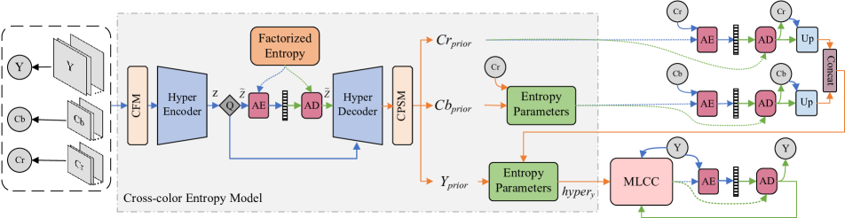
Figure 1: Overall architecture of the proposed JPEG lossless recompression method. AE and AD stands for arithmetic coding and arithmetic decoding respectively. Blue and green lines indicate data-flow for encoding and decoding respectively, orange lines are shared.

2 Related work

2.1 Overview of JPEG algorithm

JPEG algorithm first converts image from RGB sources to YCbCr color space (one luma component (Y) and two chroma components (Cb and Cr)). Then, considering human visual system is far more sensitive to brightness details stored in the luma component than to color details stored in two chroma components, the luma component is supposed to be more important than chroma components. Most JPEG images adopt YCbCr 4:2:0 format, where Y retains the same resolution while Cb and Cr components are subsampled as $\frac{1}{4}$ of their original resolution. Next, every component is divided into $8\times 8$ pixel blocks and each pixel block is transformed by discrete cosine transform (DCT) into a matrix of frequency coefficients (DCT coefficients) of the same size. Subsequently, these three components are quantized by two quantization tables: Y component uses a quantization table while Cb and Cr components share another quantization table. Finally, all DCT coefficients are compressed by lossless Huffman coding [23]. Importantly, in order to deploy Huffman coding, the two-dimensional DCT coefficients have to be turned into a one-dimensional array. Zig-zag scanning is adopted here to group similar frequencies together to obtain better performance.

2.2 JPEG recompression methods

Lepton [21] proposed by Horn et al., which achieves 22% storage reduction after recompressing JPEG losslessly, mainly focuses on optimization of entropy model and symbol representations. Instead of using Huffman coding, Lepton uses more efficient arithmetic coding [45]. Further more, combining unary, sign and absolute value, the representation method in Lepton outperforms other encodings like pure unary and two’s complement with fixed length. Lepton also deals with DC component by predicting it from AC components and storing the residual.

JPEG XL [7, 6] is a versatile compression method supporting both lossless and lossy compression. For existing JPEG images, losslessly transcoding them to JPEG XL is also supported. JPEG XL achieves better compression ratio by extending the $8\times 8$ DCT to variable-size DCT which allows block size to be one of 8, 16 or 32. Besides, JPEG XL uses Asymmetric Numeral Systems [15] in place of Huffman coding. Instead of using fixed quantization matrix globally, the quantization matrix in JEPG XL can be scaled locally to better accommodate the complexity in different areas. Compared with the primitive DC coefficient prediction mode in JPEG, JPEG XL supports eight modes and will choose the mode producing the least amount of error.

CMIX [1] is a general lossless data compression program aimed at optimizing compression ratio at the cost of high CPU/memory usage. It achieves state-of-the-art results on several compression benchmarks. CMIX uses an ensemble of independent models to predict the probability of each bit in the input stream. The model predictions are combined into a single probability using a context mixing algorithm. The output of the context mixer is refined using an algorithm called secondary symbol estimation (SSE). CMIX can compress all data files losslessly, including JPEG images.

2.3 End-to-end image compression

Learned lossy compression. Since Ballé et al. [8] proposes an end-to-end learned image compression method based on variational autoencoder [43] (VAE) architecture, subsequent deep-learning based approaches continue to explore and improve similar architectures (e.g. [9, 36, 29, 27, 13, 22, 18, 46, 19, 12, 47]). These methods initially focus on how to deal with non-differential quantization and rate estimation to enable end-to-end training [8, 36]. Then, in order to build more accurate entropy model to further reduce the cross entropy (corresponding to bit rate), some methods [9, 22] devote to introduce hyperprior models to the VAE architecture. More recent approaches investigate context models for more accurate entropy estimation, e.g. adding pixel-wise [29] or channel-wise autoregressive [30] modules. These techniques have greatly improved the performance of learned image compression. Actually, all of the learned methods mentioned above have outperformed JPEG. The performance of newest methods [18, 47] even surpasses the intra coding of latest standard VVC/H.266 [31]. However, they focus on the compression of images stored in lossless format like PNG, serving as replacement of JPEG instead of recompressing existing JPEG images.

Learned lossless compression. Our research is more related to learned lossless image compression. In theory, any probabilistic model can be used together with entropy coders to compress data into compact bitstreams losslessly. The bit rate lower bound is given by the probabilistic model according to Shannon’s landmark paper [37] (i.e. the more accurate the probabilistic model is, the lower the bit rate will be). Representative learned lossless image compression methods include likelihood-based generative models (e.g. PixelCNN [32], PixelRNN [42], MS-PixelCNN [35]), bits-back methods (e.g. BB-ANS [39], Bit-Swap [25], Hilloc [40]) and flow-based models (e.g. IDF [20], IDF++ [41], iVPF [49]). To reduce computation complexity, a parallelizable hierarchical probabilistic model is proposed in L3C [28], which is the first practical full-resolution learned lossless image compression method. This hierarchical probabilistic modeling idea is later improved by SReC [11] and the multi-scale progressive statistical model [48]. Nevertheless, same as learned lossy image compression, these learned lossless compression methods still only consider images stored in PNG format while ignoring the vast already existing JPEG images. In our investigation, we find these methods cannot be used directly to losslessly compress JPEG images, which we focus on in this work.

3 Method

3.1 Framework

The overall framework of the proposed model is presented in Fig. 1. Since DCT domain is used in our method to design an efficient entropy model, we first rearrange each $8\times 8$ block of DCT coefficients in order to learn better distribution (Sec. 3.2). Because JPEG usually adopts YCbCr 4:2:0 format, we apply a Coefficient Fusion Model (CFM) detailed in Sec. 3.3 to align the shape of DCT coefficients from different color components. After shape alignment, DCT coefficients are sent to a Hyper Encoder and will produce the hyperprior $\widetilde{z}$, which is saved in the bitstream as side information. Subsequently, the coding prior of the three color components will be obtained after the hyperprior $\widetilde{z}$ goes through Hyper Decoder and a Coefficient Prior Split Model (CPSM) detailed in Sec. 3.3.

Besides the shared hyperprior $\widetilde{z}$, we further reduce the statistical redundancy by explicitly modelling the correlation between color components and DCT coefficients. Detailed in Sec. 3.3, we estimate Cr distribution conditioned on $\widetilde{z}$, Cb distribution conditioned on both $\widetilde{z}$ and Cr, and Y distribution conditioned on $\widetilde{z}$, Cr and Cb. According to human perception, Y component contains more information than Cb and Cr components. We propose a multi-level cross-channel (MLCC) entropy enhancement model to better predict Y distribution, which is described in Sec. 3.5.

Finally, we use arithmetic coding [45] based on these probabilistic distributions to compress component coefficients into compact bitstreams losslessly.

3.2 DCT Coefficients Rearrangement

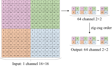
Figure 2: DCT coefficients rearrangement using a $16\times 16$ image as an example. Four $8\times 8$ DCT blocks are rearranged by frequency and zigzag scan.

JPEG encoder transforms the pixels in an $8\times 8$ block to a matrix of DCT coefficients in the same size and each coefficient in the matrix stands for one frequency. The top left corner of this matrix is the DC component, while the remaining 63 coefficients are AC components. As shown in Fig. 2, we first adopt the same way as [17] to rearrange DCT coefficients so that the same frequency from all blocks are extracted together to form the spatial dimension, and different frequencies form the channel dimension. This operation converts Y, Cb, Cr components to 64 channels with $\frac{1}{64}$ of their original spatial size. A lot of coefficients in AC components will go to zero after quantization. Therefore, we rearrange the channel dimension by zigzag scan in the original DCT matrix to make zero values as close as possible to exploit the structural information.

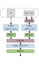
(a) CFM

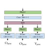
(b) CPSM

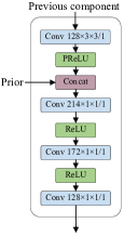
(c) Entropy Parameters

Figure 3: Detailed architecture of CFM, CPSM and Entropy Parameters network.

3.3 Cross-Color Entropy Model

Cross-color correlation can be modeled both implicitly (through shared hyperprior) and explicitly (through the entropy parameters network).

Hyperprior network proposed in [9] can be viewed as an efficient entropy model which generates hyperprior $\widetilde{z}$ as side information and then produces the scale parameters for Gaussian distribution conditioned on $\widetilde{z}$. This method is improved in their later work [29], where hyperprior is combined with context-based predictions. The same hyper-network as [29] is used in our method to extract hyperprior from fused color components, which serves as side information and models the cross-color correlation implicitly. However, this VAE-like model is unable to support YCbCr 4:2:0 format directly due to different spatial resolutions. Similar to [16], we add Coefficient Fusion Model (CFM) and Coefficient Prior Split Model (CPSM) to Hyper Encoder and Hyper Decoder respectively. Architecture of CFM is shown in Fig. 3(a), through which the three color components are reshaped and fused. As shown in Fig. 3(b), CPSM is used to split the prior of the three color components, producing $Y_{prior}$, $Cb_{prior}$ and $Cr_{prior}$.

Each element of DCT coefficients is modeled as a single Laplace distribution with its own scale $b$ and location $\mu$ parameters. We split $Cr_{prior}$ into $b_{cr}$ and $\mu_{cr}$ to obtain Laplace parameters of Cr component. $b_{cr}$ and $\mu_{cr}$ have the same size as Cr component. As formulated in Eq. 1, the probability of Cr given $\widetilde{z}$ is calculated in a factorized manner. Subsequently, Cr component is fed to Entropy Parameters network (Fig. 3(c)) as context of Cb component and is fused with $Cb_{prior}$. The output of this model is split into $b_{cb}$ and $\mu_{cb}$. As a result, the probability mass function (PMF) of Cb component will be conditioned on both Cr component and hyperprior $\widetilde{z}$ and is shown in Eq. 2.

Cb and Cr components are upsampled by $3\times 3$ stride-2 transposed convolution and concatenated to serve as context of Y component. They are fed together with $Y_{prior}$ to Entropy Parameters network and we can obtain $hyper_{y}$ (Fig. 1) to calculate the conditional distribution $p_{y|\widetilde{z},{c_{b}},{c_{r}}}(y|\widetilde{z},{c_{b}},{c_{r}})$. Nevertheless, this PMF similar to Cr and Cb components is not powerful enough for the most informative Y component. In the following section, we propose a more suitable context modelling method to further reduce redundancy in Y component.

$$p_{{c_{r}}|\widetilde{z}}({c_{r}}|\widetilde{z}) =\prod^{N}_{i=0}p\left({c_{r}}_{i}|\widetilde{z}\right)$$ (1)

$$p({c_{r}}_{i}|\widetilde{z}) =\int_{{c_{r}}_{i}-\frac{1}{2}}^{{c_{r}}_{i}+\frac{1}{2}}Laplace({c_{r}}^{\prime}|\mu_{{c_{r}}_{i}},b_{{c_{r}}_{i}})\,d{c_{r}}^{\prime}$$

$$p_{{c_{b}}|\widetilde{z},{c_{r}}}({c_{b}}|\widetilde{z},{c_{r}}) =\prod^{N}_{i=0}p\left({c_{b}}_{i}|\widetilde{z},{c_{r}}\right)$$ (2)

$$p({c_{b}}_{i}|\widetilde{z},{c_{r}}) =\int_{{c_{b}}_{i}-\frac{1}{2}}^{{c_{b}}_{i}+\frac{1}{2}}Laplace({c_{b}}^{\prime}|\mu_{{c_{b}}_{i}},b_{{c_{b}}_{i}})\,d{c_{b}}^{\prime}$$

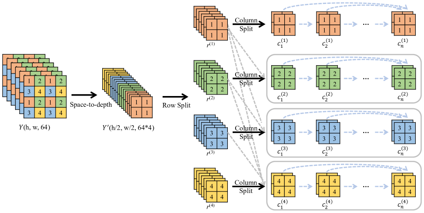
Figure 4: Matrix representation of our parallel context modelling method. Solid arrows indicate data operation and dotted arrows denote conditional relationships. Light grey and light blue dotted arrows align with Outer Channel and Inner Channel in Fig. 5, respectively.

3.4 Matrix Context Model

Context modeling is an efficient technique to predict precise probabilistic distribution of unknown symbols based on adjacent symbols that have already been decoded. Previous learning-based codecs adopt a spatially auto-regressive context model, which requires decoding each symbol sequentially. While these methods are effective, they are impractical for real-world deployment due to low computational efficiency caused by the lack of parallelization [29, 24]. Then, channel-conditional (CC) context models are explored in [30], which splits the symbol tensor along channel dimension into many equal-size slices and each slice can be modeled conditioned on all already decoded slices, providing much better parallelism. Subsequently, He et al. [19] proposes a novel spatial parallel context model with a two-pass decoding approach, where the symbol tensor is decomposed into two groups according to checkerboard pattern and then one group serves as context of the other to build conditional distribution. Meanwhile, a hierarchical probabilistic modeling idea, which is similar in spirit to spatially parallel context model, is prevalent in learned lossless image compression. Hierarchical models [28, 11, 48] downsample an input image into different low-resolution representations and the probabilistic distribution of the input image is the product of the conditional distributions in multiple scales.

In this paper, we propose a novel parallelizable matrix context model to enhance the entropy estimation of Y component. As shown in Fig. 4, we first use space-to-depth operation (i.e. inverse operation of PixelShuffle [38]) to convert Y component to $Y^{\prime}$ ($64\times 4$ channels with $\frac{1}{4}$ of the original spatial size). Then we partition $Y^{\prime}$ along channel dimension into 4 equal-size slices (i.e. 4 rows in the matrix representation, $Y^{\prime}={r^{(1)}\bigcup r^{(2)}\bigcup r^{(3)}\bigcup r^{(4)}}$), where each row is modeled conditioned on all previously decoded rows. Therefore, the conditional distribution $p_{y|\widetilde{z},{c_{b}},{c_{r}}}(y|\widetilde{z},{c_{b}},{c_{r}})$ can be calculated as:

$$p_{y|\widetilde{z},{c_{b}},{c_{r}}}(y|\widetilde{z},{c_{b}},{c_{r}})$$ (3)

$$= p_{y|\widetilde{z},{c_{b}},{c_{r}}}(r^{(1)},r^{(2)},r^{(3)},r^{(4)}|\widetilde{z},{c_{b}},{c_{r}})$$

$$= \prod^{4}_{i=1}p\left(r^{(i)}|r^{(i-1)},\cdots,r^{(1)},\widetilde{z},{c_{b}},{c_{r}}\right)$$

Each row has 64 channels and there exists considerable redundancy. Hence, each row is further partitioned to explicitly exploit this channel-wise correlation, i.e. $r^{(i)}=c^{(i)}_{1}\bigcup c^{(i)}_{2}\bigcup\cdots\bigcup c^{(i)}_{n}$, where $n$ is the number of split columns at row $i$. Let $R^{(i)}=\left\{r^{(i-1)},\cdots,r^{(1)},\widetilde{z},{c_{b}},{c_{r}}\right\}$ denote the context and prior for $r^{(i)}$ (specifically, $R^{(1)}=\left\{\widetilde{z},{c_{b}},{c_{r}}\right\}$), we can further factorize Eq. 3 based on

$$p\left(r^{(i)}|R^{(i)}\right)=\prod^{n}_{j=1}p\left(c^{(i)}_{j}|c^{(i)}_{j-1},\cdots,c^{(i)}_{1},R^{(i)}\right)$$ (4)

where $c^{(i)}_{j}$ is column $j$ at row $i$, $n$ is the number of columns at row $i$, and $i=1,2,3,4$.

Let $C^{(i)}_{j}=\left\{c^{(i)}_{1},\cdots,c^{(i)}_{j-1},R^{(i)}\right\}$ denote the context and prior for column $j$ at row $i$ (specifically, $C^{(i)}_{1}=\left\{R^{(i)}\right\}$) and coefficients within a column are conditionally independent and estimated by single Laplace model in parallel, we can further factorize Eq. 4 based on Eq. 5. Laplace parameters are derived from $C^{(i)}_{j}$ according to Sec. 3.5.

$$p\left(c^{(i)}_{j}|C^{(i)}_{j}\right)=\prod^{m_{j}}_{k=1}p\left(y^{(i)}_{jk}|C^{(i)}_{j}\right)$$ (5)

$$p\left(y^{(i)}_{jk}|C^{(i)}_{j}\right)=\int_{y^{(i)}_{jk}-\frac{1}{2}}^{y^{(i)}_{jk}+\frac{1}{2}}Laplace(y^{\prime}|\mu_{y^{(i)}_{jk}},b_{y^{(i)}_{jk}})\,dy^{\prime}$$

where $y^{(i)}_{jk}$ is coefficient $k$ in column $j$ at row $i$, $m_{j}$ is the number of coefficients in column $j$, $i=1,2,3,4$, $j=1,2,\cdots,n$, and $k=1,2,\cdots,m_{j}$.

According to the rearrangement in Sec. 3.2, the 64 channels at each row in our matrix context model represent different frequency, where higher frequency has been quantized more aggressively and contains less information. Therefore, we reverse the channel order in each row when formulating the matrix context (i.e. $c^{(i)}_{1}$ in Fig. 4 is the AC coefficients representing the highest frequency in $r^{(i)}$). Moreover, we design non-uniform partition for the column dimension to balance this information asymmetry. Specifically, we let the number of columns be n=9, the lengths of each column ($c^{(i)}_{j},j=1,2,\cdots,9$) are set as 28, 8, 7, 6, 5, 4, 3, 2 and 1 respectively.

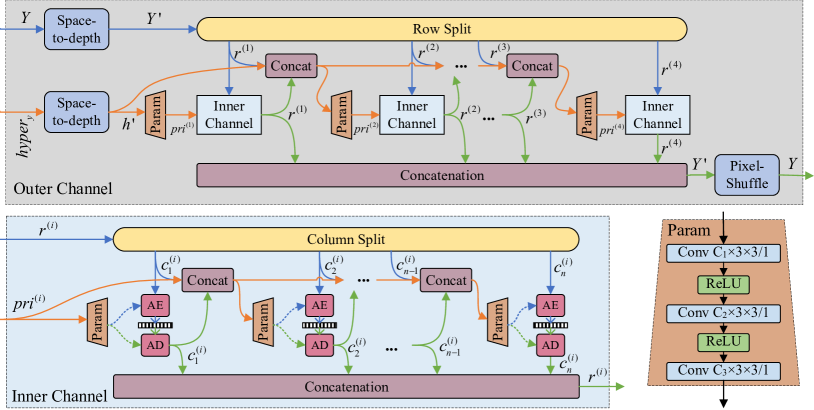
Figure 5: Detailed data-flow for applying multi-level cross-channel (MLCC) model. Letting $n$, $m$ representing the channel number of input tensor and next slice to be modeled respectively, $C_{1}$, $C_{2}$ and $C_{3}$ are decided by $C_{1}=n-d,C_{2}=n-2*d,C_{3}=2*m,d=(n-2*m)//3$. Blue and green lines indicate data-flow for encoding and decoding respectively, orange lines are shared.

3.5 Multi-Level Cross-Channel Entropy Model

A deep neural network named Multi-Level Cross-Channel (MLCC) is designed to implement our matrix context entropy model to estimate Laplace parameters (location $\mu$ and scale $b$) in Eq. 5, where we interpret the matrix context model as cross-channel autoregressive model: autoregression along the rows is viewed as Outer Channel (top in Fig. 5) to generate prior of each row (i.e. $pri^{(i)}$ in Fig. 5), autoregression along the columns in each row is modeled as Inner Channel (bottom left in Fig. 5) to generate Laplace parameters for each column. MLCC leverages both matrix context and $hyper_{y}$ (Sec. 3.3) to learn more powerful PMF for the most informative Y component.

As shown in Fig. 5, We first adopt space-to-depth to rearrange $hyper_{y}$ into $h^{\prime}$ as prior of Outer Channel ($h^{\prime}$ has $64\times 4$ channels with $\frac{1}{4}$ spatial size of $hyper_{y}$). Meanwhile, Y component is reshaped by space-to-depth and then split into 4 rows (Sec. 3.4), the first row $r^{(1)}$ is predicted conditioned solely on $h^{\prime}$. However, unlike [30], this step in our method will generate prior $pri^{(i)}$ for current row $r^{(i)}$ rather than entropy parameters. Next, the current row and its own $pri^{(i)}$ are sent to Inner Channel. In Inner Channel model, the row is partitioned into $n$ columns (we set $n$ to 9 in our method). And then the first column is compressed using a single Laplace entropy model with mean and scale conditioned only on $pri^{(i)}$, while the entropy model for the remaining columns (e.g. $c^{(i)}_{j}$) are conditioned on $pri^{(i)}$ and all decoded coefficients in previous columns (e.g. $\left\{c^{(i)}_{1},\cdots,c^{(i)}_{j-1}\right\}$). After all columns in current row are decoded by Inner Channel model, they will be concatenated with $h^{\prime}$ and all previously decoded rows, and then processed by Outer Channel model again to generate prior $pri^{(i+1)}$ for next row $r^{(i+1)}$. Repeat this operation until all rows in Y component is encoded or decoded.

With this MLCC model, decoding will be slower than encoding because of the conditional relationship. In decoding stage those columns and rows must be decoded sequentially. However, all the coefficients in the same column can be processed in parallel, ensuring that the overall sequential complexity is constant (irrelevant of the input image size), which is $4\times n$ (we let the number of columns be n=9). This guarantees that our method can be practical for recompressing high resolution JPEG images.

3.6 Loss Function

The expected code length arithmetic coding [45] can achieve, using our learned distribution as its probability model, is given by the cross entropy:

$$R =\mathbb{E}_{\widetilde{z}\sim\widetilde{p}_{\widetilde{z}}}\left[-\log_{2}p_{\widetilde{z}}(\widetilde{z})\right]+\mathbb{E}_{{c_{r}}\sim\widetilde{p}_{{c_{r}}|\widetilde{z}}}\left[-\log_{2}p_{{c_{r}}|\widetilde{z}}({c_{r}}|\widetilde{z})\right]$$ (6)

$$+\mathbb{E}_{{c_{b}}\sim\widetilde{p}_{{c_{b}}|\widetilde{z},{c_{r}}}}\left[-\log_{2}p_{{c_{b}}|\widetilde{z},{c_{r}}}({c_{b}}|\widetilde{z},{c_{r}})\right]$$

$$+\mathbb{E}_{y\sim\widetilde{p}_{y|\widetilde{z},{c_{b}},{c_{r}}}}\left[-\log_{2}p_{y|\widetilde{z},{c_{b}},{c_{r}}}(y|\widetilde{z},{c_{b}},{c_{r}})\right]$$

where $\widetilde{p}$ is the true distribution of DCT coefficients, $p$ is estimated by entropy model. Our model is trained to minimize this cross entropy to minimize the bit-length.

4 Experiments

4.1 Settings

Datasets. The training dataset comprises the largest 8000 images chosen from the ImageNet [14] validation set, where each image contains more than one million pixels. Similar to [8, 9, 19], each image is disturbed by uniform noise and downsampled. We evaluate our model on four datasets: Kodak [26] dataset with 24 images, 100 images chosen from DIV2K [4], CLIC [3] professional test dataset with 250 images and CLIC mobile dataset with 178 images. Since our method processes images entirely in DCT domain, before fed to model, we use torchjpeg.codec.quantize_at_quality [2] to extract quantized DCT coefficients with given JPEG quality level, which guarantees that the result is the same as using JPEG images generated from image libraries like Pillow. We fix the quality level of the training dataset at $75$ if not specified.

Implementation details. During training, $256\times 256$ pixel patches are randomly cropped from training data and then quantized DCT coefficients are extracted. Our model is implemented in PyTorch [33] and we adopt Adam optimizer. The batch-size is $16$ and the learning-rate is $10^{-4}$. We apply gradient clipping for the sake of stability and train the model for $2000$ epochs. All the speed testing results are obtained on single Nvidia GeForce GTX 1060 6GB (GPU) for learned methods and Intel(R) Xeon(R) CPU E5-2620 v4 @ 2.10GHz (CPU) for non-learned ones.

4.2 Performance

Performance comparison with other JPEG recompression methods. We compare the proposed model against other state-of-the-art methods for JPEG recompression on four test datasets mentioned in Sec. 4.1. We adopt our best model with $9$ non-uniform channel slices, where the number of channels is split as $[28,8,7,6,5,4,3,2,1]$. As shown in Tab. 1, with quality level set as 75, our method achieves lowest bit rate on all evaluation datasets and obtains about $30\%$ compression savings. Our method is much faster than CMIX but slower than JPEG XL and Lepton. However, it is worth noticing that our implementation of arithmetic coder is naive and our model has not been optimized to achieve the fastest speed.

Performance on different quality levels. We test our models on Kodak with $7$ different JPEG quality levels (i.e. $quality=35,45,55,65,75,85,95$). The results are presented in Fig. 6. It shows that our method still outperforms other methods, which shows that our model trained for $quality=75$ can generalize well to different quality levels except very high quality like 95. More detailed results are given in the appendix.

Performance comparison with other learned lossless compression methods. We compare our method with representative learned lossless image compression methods designed for PNG images, including IDF [20] and multi-scale model [48]. These methods are designed for RGB 4:4:4 format, so we convert JPEG 4:2:0 input data to RGB 4:4:4 format by upsampling Cb and Cr components. This upsampling operation increases resolution and may cause unfair comparison. Consequently, we also carry out experiments with JPEG 4:4:4 source format and convert it to RGB 4:4:4 as model input. By modifying these models slightly, these methods can also deal with JPEG 4:2:0 format directly, we present results of this kind of experiments in the appendix.

As shown in Tab. 2, both for JPEG 4:2:0 and JPEG 4:4:4 format, our models outperform IDF and multi-scale model by a large margin. Additionally, we evaluate neural network latency of our model, L3C [28], IDF [20] and multi-scale [48] in Fig. 7, which shows our model is faster.

	BPP and Savings (%)				time (s)
Method	Kodak	DIV2K	CLIC.mobile	CLIC.pro	Encoding	Decoding
JPEG [44]	1.369	1.285	1.099	0.922	-	-
Lepton [21]	1.102 $(19.50\%)$	1.017 $(20.86\%)$	0.863 $(21.47\%)$	0.701 $(23.97\%)$	0.239	0.127
JPEG XL [7, 6]	1.173 $(16.70\%)$	1.072 $(16.58\%)$	0.908 $(17.38\%)$	0.744 $(19.30\%)$	0.179	0.125
CMIX [1]	1.054 $(23.01\%)$	0.931 $(27.55\%)$	0.804 $(26.84\%)$	0.648 $(29.72\%)$	152.9	154.5
Ours	0.965 $(29.51\%)$	0.892 $(30.58\%)$	0.772 $(29.75\%)$	0.624 $(32.32\%)$	1.131	1.023

Table 1: Performance comparison on various datasets. The encoding and decoding time are evaluated on Kodak with QP 75.

Source format	Method	Input format	BPP
JPEG 4:2:0	Multi-scale [48]	RGB 4:4:4	4.398
	IDF [20]	RGB 4:4:4	6.964
	Ours	DCT 4:2:0	0.965
JPEG 4:4:4	Multi-scale [48]	RGB 4:4:4	4.604
	IDF [20]	RGB 4:4:4	7.059
	Ours	DCT 4:4:4	1.122

Table 2: Performance comparison with learned lossless compression methods.

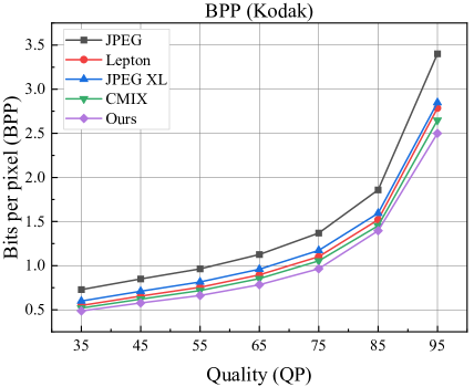
Figure 6: Comparison of bits per pixel (BPP) on Kodak dataset when recompressing JPEG images of different quality levels (QP). At QP 95, we use the model trained with QP 95. At other points, we use the model trained with QP 75.

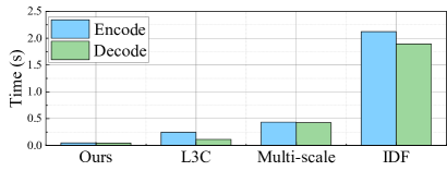
Figure 7: Time spent on neural networks compared with representative learned lossless compression methods. These models are evaluated on Kodak in JPEG 4:4:4 with QP 75.

4.3 Ablation study

We test a serial of models on Kodak with quality level 75 to investigate the effect of cross-color entropy model, multi-level cross-channel entropy enhancement model and non-uniform channel slices.

Method	Parameters	BPP	Savings
Ours	32.3M	0.965	29.51%
Cross-color case 1	36.9M	0.983	28.20%
Cross-color case 2	31.5M	0.973	28.93%
Cross-color case 3	88.0M	0.968	29.29%
Only Outer Channel	22.5M	1.027	24.98%
Only Inner Channel	9.1M	1.012	26.08%
Column-to-row	13.0M	0.988	27.83%
Uniform 8 slices	30.0M	0.986	27.98%
Non-uniform 8 slices	31.5M	0.966	29.44%

Table 3: Ablation study.

Effectiveness of cross-color entropy model. To verify the effectiveness of our cross-color entropy model, we compare three models. Cross-color case 1: Y, Cb, and Cr components are modeled totally independent of each other, i.e. there are three side information $\widetilde{z}_{Y},\widetilde{z}_{Cb},\widetilde{z}_{Cr}$, and Y (with MLCC), Cb and Cr components are dependent on $\widetilde{z}_{Y},\widetilde{z}_{Cb},\widetilde{z}_{Cr}$ respectively. Cross-color case 2: Hyperprior $\widetilde{z}$ is shared by Y, Cb, and Cr components, and these three color components are conditioned on the shared $\widetilde{z}$ except that the entropy model of Y component is enhanced by MLCC. Here $\widetilde{z}$ provides implicit cross-color correlation while no explicit modeling is used. Cross-color case 3: Three color components are modeled totally independent of each other, while they are treated equally and are all modeled by independent hyperprior with corresponding MLCC module. We give detailed architectures in the appendix. As shown in Tab. 3, savings of case 1 and case 2 are lower than our proposed model and case 2 is better than case 1, indicating that both implicit and explicit cross-color correlation modeling is helpful to bit saving. Although the network capacity and parameter number are the largest in case 3, its performance is still slightly worse than our model, proving the effectiveness of our cross-color entropy model.

Effectiveness of MLCC model. To verify the effectiveness of MLCC, we replace MLCC with three different models while keeping other parts of the model unchanged. Only Outer Channel drops the Inner Channel module in MLCC, which means there are no column split operation. Only Inner Channel has no space-to-depth and row split operations, which only has Inner Channel module in MLCC. Column-to-row is a variation of our row-to-column MLCC, which adopts column split first and then row split. Details about these models are given in the appendix. Shown in Tab. 3, the above three replacements of MLCC deteriorate the compression savings, which verifies the effectiveness of MLCC.

Effectiveness of non-uniform slices. We compare two models to verify that non-uniform column slicing in MLCC is more effective for JPEG recompression. Uniform 8 slices divides rows evenly into $8$ columns, while non-uniform 8 slices divides rows into $8$ columns of size $[36,7,6,5,4,3,2,1]$ respectively. As demonstrated in Tab. 3, non-uniform 8 slices model has the same column number as uniform 8 slices model but its compression ratio is about $1.5\%$ higher.

5 Conclusion

We propose a novel Multi-Level Cross-Channel entropy model for lossless recompression of existing JPEG images, which achieves state-of-the-art performance on Kodak, DIV2K, CLIC.mobile and CLIC.pro and has reasonable running speed. We also show that our method trained with quality level 75 can generalize well on other quality levels except very high quality like 95. To the best of our knowledge, this is the first learned method targeting lossless recompression of JPEG images. For future work, we will explore the generalizability on very high quality levels.

References

- [1] Cmix. https://www.byronknoll.com/cmix.html.
- [2] torchjpeg.codec. https://queuecumber.gitlab.io/torchjpeg/api/torchjpeg.codec.html.
- [3] Workshop and challenge on learned image compression. https://www.compression.cc/challenge/.
- [4] Eirikur Agustsson and Radu Timofte. Ntire 2017 challenge on single image super-resolution: Dataset and study. In Proceedings of the IEEE conference on computer vision and pattern recognition workshops, pages 126–135, 2017.
- [5] Nasir Ahmed, T_ Natarajan, and Kamisetty R Rao. Discrete cosine transform. IEEE transactions on Computers, 100(1):90–93, 1974.
- [6] Jyrki Alakuijala, Sami Boukortt, Touradj Ebrahimi, Evgenii Kliuchnikov, Jon Sneyers, Evgeniy Upenik, Lode Vandevenne, Luca Versari, and Jan Wassenberg. Benchmarking jpeg xl image compression. In Optics, Photonics and Digital Technologies for Imaging Applications VI, volume 11353, page 113530X. International Society for Optics and Photonics, 2020.
- [7] Jyrki Alakuijala, Ruud van Asseldonk, Sami Boukortt, Martin Bruse, Iulia-Maria Comșa, Moritz Firsching, Thomas Fischbacher, Evgenii Kliuchnikov, Sebastian Gomez, Robert Obryk, et al. Jpeg xl next-generation image compression architecture and coding tools. In Applications of Digital Image Processing XLII, volume 11137, page 111370K. International Society for Optics and Photonics, 2019.
- [8] Johannes Ballé, Valero Laparra, and Eero P Simoncelli. End-to-end optimized image compression. In Int. Conf. on Learning Representations, 2017.
- [9] Johannes Ballé, David Minnen, Saurabh Singh, Sung Jin Hwang, and Nick Johnston. Variational image compression with a scale hyperprior. In International Conference on Learning Representations, 2018.
- [10] Fabrice Bellard. Bpg image format. https://bellard.org/bpg.
- [11] Sheng Cao, Chao-Yuan Wu, and Philipp Krähenbühl. Lossless image compression through super-resolution. arXiv preprint arXiv:2004.02872, 2020.
- [12] Tong Chen, Haojie Liu, Zhan Ma, Qiu Shen, Xun Cao, and Yao Wang. End-to-end learnt image compression via non-local attention optimization and improved context modeling. IEEE Transactions on Image Processing, 30:3179–3191, 2021.
- [13] Zhengxue Cheng, Heming Sun, Masaru Takeuchi, and Jiro Katto. Learned image compression with discretized gaussian mixture likelihoods and attention modules. In Proceedings of the IEEE/CVF Conference on Computer Vision and Pattern Recognition (CVPR), June 2020.
- [14] Jia Deng, Wei Dong, Richard Socher, Li-Jia Li, Kai Li, and Li Fei-Fei. Imagenet: A large-scale hierarchical image database. In 2009 IEEE conference on computer vision and pattern recognition, pages 248–255. Ieee, 2009.
- [15] Jarek Duda, Khalid Tahboub, Neeraj J Gadgil, and Edward J Delp. The use of asymmetric numeral systems as an accurate replacement for huffman coding. In 2015 Picture Coding Symposium (PCS), pages 65–69. IEEE, 2015.
- [16] Hilmi E Egilmez, Ankitesh K Singh, Muhammed Coban, Marta Karczewicz, Yinhao Zhu, Yang Yang, Amir Said, and Taco S Cohen. Transform network architectures for deep learning based end-to-end image/video coding in subsampled color spaces. arXiv preprint arXiv:2103.01760, 2021.
- [17] Max Ehrlich, Larry Davis, Ser-Nam Lim, and Abhinav Shrivastava. Quantization guided jpeg artifact correction. In Computer Vision–ECCV 2020: 16th European Conference, Glasgow, UK, August 23–28, 2020, Proceedings, Part VIII 16, pages 293–309. Springer, 2020.
- [18] Zongyu Guo, Zhizheng Zhang, Runsen Feng, and Zhibo Chen. Causal contextual prediction for learned image compression. IEEE Transactions on Circuits and Systems for Video Technology, 2021.
- [19] Dailan He, Yaoyan Zheng, Baocheng Sun, Yan Wang, and Hongwei Qin. Checkerboard context model for efficient learned image compression. In Proceedings of the IEEE/CVF Conference on Computer Vision and Pattern Recognition, pages 14771–14780, 2021.
- [20] Emiel Hoogeboom, Jorn Peters, Rianne van den Berg, and Max Welling. Integer discrete flows and lossless compression. Advances in Neural Information Processing Systems, 32:12134–12144, 2019.
- [21] Daniel Reiter Horn, Ken Elkabany, Chris Lesniewski-Laas, and Keith Winstein. The design, implementation, and deployment of a system to transparently compress hundreds of petabytes of image files for a file-storage service. In Proceedings of the 14th USENIX Conference on Networked Systems Design and Implementation, pages 1–15, 2017.
- [22] Yueyu Hu, Wenhan Yang, and Jiaying Liu. Coarse-to-fine hyper-prior modeling for learned image compression. In Proceedings of the AAAI Conference on Artificial Intelligence, volume 34, pages 11013–11020, 2020.
- [23] David A Huffman. A method for the construction of minimum-redundancy codes. Proceedings of the IRE, 40(9):1098–1101, 1952.
- [24] Nick Johnston, Elad Eban, Ariel Gordon, and Johannes Ballé. Computationally efficient neural image compression. arXiv preprint arXiv:1912.08771, 2019.
- [25] Friso Kingma, Pieter Abbeel, and Jonathan Ho. Bit-swap: Recursive bits-back coding for lossless compression with hierarchical latent variables. In International Conference on Machine Learning, pages 3408–3417. PMLR, 2019.
- [26] Eastman Kodak. Kodak lossless true color image suite (photocd pcd0992). http://r0k.us/graphics/kodak/, 1993.
- [27] Jooyoung Lee, Seunghyun Cho, and Seung-Kwon Beack. Context-adaptive entropy model for end-to-end optimized image compression. In International Conference on Learning Representations, 2018.
- [28] Fabian Mentzer, Eirikur Agustsson, Michael Tschannen, Radu Timofte, and Luc Van Gool. Practical full resolution learned lossless image compression. In Proceedings of the IEEE/CVF conference on computer vision and pattern recognition, pages 10629–10638, 2019.
- [29] David Minnen, Johannes Ballé, and George D Toderici. Joint autoregressive and hierarchical priors for learned image compression. In Advances in Neural Information Processing Systems, pages 10771–10780, 2018.
- [30] David Minnen and Saurabh Singh. Channel-wise autoregressive entropy models for learned image compression. In 2020 IEEE International Conference on Image Processing (ICIP), pages 3339–3343. IEEE, 2020.
- [31] Jens-Rainer Ohm and Gary J Sullivan. Versatile video coding–towards the next generation of video compression. In Picture Coding Symposium, volume 2018, 2018.
- [32] Aäron van den Oord, Nal Kalchbrenner, Oriol Vinyals, Lasse Espeholt, Alex Graves, and Koray Kavukcuoglu. Conditional image generation with pixelcnn decoders. In Proceedings of the 30th International Conference on Neural Information Processing Systems, pages 4797–4805, 2016.
- [33] Adam Paszke, Sam Gross, Francisco Massa, Adam Lerer, James Bradbury, Gregory Chanan, Trevor Killeen, Zeming Lin, Natalia Gimelshein, Luca Antiga, et al. Pytorch: An imperative style, high-performance deep learning library. In Advances in Neural Information Processing Systems, pages 8024–8035, 2019.
- [34] Majid Rabbani. Jpeg2000: Image compression fundamentals, standards and practice. Journal of Electronic Imaging, 11(2):286, 2002.
- [35] Scott Reed, Aäron Oord, Nal Kalchbrenner, Sergio Gómez Colmenarejo, Ziyu Wang, Yutian Chen, Dan Belov, and Nando Freitas. Parallel multiscale autoregressive density estimation. In International Conference on Machine Learning, pages 2912–2921. PMLR, 2017.
- [36] Oren Rippel and Lubomir Bourdev. Real-time adaptive image compression. In International Conference on Machine Learning, pages 2922–2930. PMLR, 2017.
- [37] Shannon and E. C. A mathematical theory of communication. Bell Systems Technical Journal, 27(4):623–656, 1948.
- [38] Wenzhe Shi, Jose Caballero, Ferenc Huszár, Johannes Totz, Andrew P Aitken, Rob Bishop, Daniel Rueckert, and Zehan Wang. Real-time single image and video super-resolution using an efficient sub-pixel convolutional neural network. In Proceedings of the IEEE conference on computer vision and pattern recognition, pages 1874–1883, 2016.
- [39] James Townsend, Thomas Bird, and David Barber. Practical lossless compression with latent variables using bits back coding. In International Conference on Learning Representations, 2018.
- [40] James Townsend, Thomas Bird, Julius Kunze, and David Barber. Hilloc: Lossless image compression with hierarchical latent variable models. arXiv preprint arXiv:1912.09953, 2019.
- [41] Rianne van den Berg, Alexey A Gritsenko, Mostafa Dehghani, Casper Kaae Sønderby, and Tim Salimans. Idf++: Analyzing and improving integer discrete flows for lossless compression. In International Conference on Learning Representations, 2020.
- [42] Aaron Van Oord, Nal Kalchbrenner, and Koray Kavukcuoglu. Pixel recurrent neural networks. In International Conference on Machine Learning, pages 1747–1756. PMLR, 2016.
- [43] Pascal Vincent, Hugo Larochelle, Yoshua Bengio, and Pierre-Antoine Manzagol. Extracting and composing robust features with denoising autoencoders. In Proceedings of the 25th international conference on Machine learning, pages 1096–1103, 2008.
- [44] Gregory K Wallace. The jpeg still picture compression standard. IEEE transactions on consumer electronics, 38(1):xviii–xxxiv, 1992.
- [45] Ian H. Witten, Radford M. Neal, and John G. Cleary. Arithmetic coding for data compression. Commun. ACM, 30(6):520–540, June 1987.
- [46] Liang Yuan, Jixiang Luo, Shaohui Li, Wenrui Dai, Chenglin Li, Junni Zou, and Hongkai Xiong. Learned image compression with channel-wise grouped context modeling. In 2021 IEEE International Conference on Image Processing (ICIP), pages 2099–2103. IEEE, 2021.
- [47] Zhongzheng Yuan, Haojie Liu, Debargha Mukherjee, Balu Adsumilli, and Yao Wang. Block-based learned image coding with convolutional autoencoder and intra-prediction aided entropy coding. In 2021 Picture Coding Symposium (PCS), pages 1–5. IEEE, 2021.
- [48] Honglei Zhang, Francesco Cricri, Hamed R Tavakoli, Nannan Zou, Emre Aksu, and Miska M Hannuksela. Lossless image compression using a multi-scale progressive statistical model. In Proceedings of the Asian Conference on Computer Vision, 2020.
- [49] Shifeng Zhang, Chen Zhang, Ning Kang, and Zhenguo Li. ivpf: Numerical invertible volume preserving flow for efficient lossless compression. In Proceedings of the IEEE/CVF Conference on Computer Vision and Pattern Recognition, pages 620–629, 2021.