Rapid Scalable Distributed Power Flow with Open-Source Implementation

Abstract

This paper introduces a new method for solving the distributed ac power flow (pf)problem by further exploiting the problem formulation. We propose a new variant of the aladin algorithm devised specifically for this type of problem. This new variant is characterized by using a reduced modelling method of the distributed ac pf problem, which is reformulated as a zero-residual least-squares problem with consensus constraints. This pf is then solved by a Gauss-Newton based inexact aladin algorithm presented in the paper. An open-source implementation of this algorithm, called rapidpf+, is provided. Simulation results, for which the power system’s dimension varies from 53 to 10224 buses, show great potential of this combination in the aspects of both the computing time and scalability.

I Introduction

The ongoing implementation of the energy transition leads to heterogeneous energy networks with numerous energy producers, energy consumers, transport, conversion and storage systems. Due to strongly varying renewable-based energy feed-ins and demands of the power system, new challenges arise in the aspect of power flow analysis, including power flow (pf)problems and optimal power flow (opf)problems.

The conventional pf problem is modeled as a system of nonlinear equations. Usually, it is solved by centralized methods, i.e., Gauss-Seidel or Newton-Raphson (Grainger, 1999). However, the centralized approach requires one central entity, where all generation information and network topology data are collected. Sharing such data is unsatisfactory for system operators. In contrast to the centralized approach, the distributed approach first solves each decoupled sub-problem in its own local agent respectively, and then deals with a coupled problem in a central coordinator, in which only little information is acquired. As a result, the distributed approach not only preserves the information privacy and decision independence, but also decreases the vulnerability due to single-point-of failure (Mühlpfordt et al., 2021).

The most well-known distributed algorithms for power flow analysis are Optimality Condition Decomposition (ocd)proposed by Hug-Glanzmann and Andersson (2009), Auxiliary Problem Principle (app)by Baldick et al. (1999), and Alternating direction method of multipliers (admm)by Erseghe (2014). In this context, ocd follows the idea of Lagrangian Relaxation Decomposition. Under certain assumptions, which cannot be guaranteed in general, it can converge to a solution with slight deviation to the optimizer. Different from ocd, app and admm introduce Augmented Lagrangian Relaxation techniques to improve convergence behaviors, while admm outperforms app by reducing the communication effort. Although admm has drawn significant attention for power flow analysis (Erseghe, 2014; Kim and Baldick, 2000; Guo et al., 2016), it normally takes quite a few iterates to approach a solution with moderate accuracy. Lately, Sun and Sun (2021) proposed a two-level admm for solving distributed ac opf problem with convergence guarantee. Nonetheless, the power flow model is formulated as a Quadratically Constrained Quadratic Program (qcqp)problem at the expense of accuracy, and the algorithm converges to a modest accuracy slowly.

In addition, Houska et al. (2016) proposed the Augmented Lagrangian based Alternating Direction Inexact Newton method (aladin)that is devised for non-convex problems with local convergence guarantee. It has found widespread application for power flow analysis of small- and medium-sized power systems (Engelmann et al., 2018; Meyer-Huebner et al., 2019; Du et al., 2019). aladin shares the same idea with admm—update primal variables in an alternating fashion. However aladin requires sensitivities information of sub-problems to build a second-order approximation in the coordinator. When using suitable Hessian approximation, aladin can achieve locally quadratic convergence. In our previous work (Mühlpfordt et al., 2021), an open-source matlab code for rapid prototyping for distributed power flow (rapidpf) is provided, in which the ac pf problem is reformulated as a zero-residual least-squares problem tailored for the aladin to speed up the convergence—all the example cases can converge within half-dozen iterates. Nevertheless, the total computing time is not acceptable for large-scale problems due to the relative large dimension of the decoupled nlp problem and the problematic code efficiency of aladin-$\alpha$ toolbox (Engelmann et al., 2020).

The contribution of the present paper is two-fold. We propose a Gauss-Newton based aladin algorithm for solving the zero-residual least-squares problem and a reduced modelling method for distributed ac pf. Based on them, we upgrade the open-source code of rapidpf. The remainder of this paper is organized as follows: Section II formulates the distributed ac pf as a zero-residual least-squares problem. Section III presents both the standard aladin and the Gauss-Newton based aladin algorithms. The upgrade of rapidpf, called rapidpf+, is described in Section IV. The simulation results are compared and discussed in Section V.

II Problem Formulation

This section introduces the distributed ac pf problem of polar voltage coordination and its zero-residual least-squares formulation. Before further discussion, we first introduce some nomenclature. For a power system, $\setRegion$ represents the set of regions, $\nregions$ is the number of regions and $\nconnections$ is the number of all the connecting tie lines between regions. In a specific region $\ell$, $\setBus_{\ell}$ is the set of all buses, whereas $\setBus^{core}_{\ell}$ and $\setBus^{copy}_{\ell}$ are the set of core and copy buses in this region $\ell$, respectively.

II-A Distributed Power Flow

The conventional ac pf problem seeks a deterministic solution to the steady-state operation of an ac electrical power system by applying numerical analysis techniques (Frank and Rebennack, 2016). Each bus in the system has four variables, i.e., voltage angle $\vang$, voltage magnitude $\vmag$, active power injection $\p$, and reactive power injection $\q$.

(a) Coupled system

(b) Decoupled region 2

(c) Decoupled region 2

Figure 1: Decomposition by sharing components for a two-region system

Fact 1

Genetically, there are multiple mathematically valid solutions to a power flow problem, but only one solution has physical meaning (Frank and Rebennack, 2016).This results, e.g., from the periodic voltage angle $\vang$, and the respective trigonometric functions.

In order to apply a distributed algorithm, reformulation of the ac pf problem is necessary. In terms of partitioning the power system, we share the components between neighboring regions to ensure physical consistency. As an example, we take the 6-bus system with 2 regions, shown in Figure 1. The coupled system, shown in Figure 1(a), has been partitioned into 2 local regions. To solve the ac pf problem in region $R_{1}$, besides its own buses {1,2,3} called core buses, the complex voltage of bus {4} from neighboring region $R_{2}$ is required. Hence, for the sub-problem of region $R_{1}$, we create an auxiliary bus {4} called copy bus, along with its own core bus, to formulate a self-contained ac pf problem.

Then, affine consensus constraints of the connecting tie line are added to ensure consistency of the copy bus with its original core bus in the neighboring region. The consensus constraints of the example case in Figure 1 can be written as

$$\vang^{\textrm{core}}_{3}=\vang^{\textrm{copy}}_{3}, \;\vang^{\textrm{core}}_{4}=\vang^{\textrm{copy}}_{4}$$ (1a)

$$\vmag^{\textrm{core}}_{3}=\vmag^{\textrm{copy}}_{3}, \;\vmag^{\textrm{core}}_{4}=\vmag^{\textrm{copy}}_{4}$$ (1b)

In a specific region $\ell$, the power flow equations be represented as

$$\p_{i}^{g}-\p_{i}^{l} =\vmag_{i}\sum_{k\in\setBus_{\ell}}\vmag_{k}\left(G_{ik}\cos\vang_{ik}+B_{ik}\sin\vang_{ik}\right)$$ (2a)

$$\q_{i}^{g}-\q_{i}^{l} =\vmag_{i}\sum_{k\in\setBus_{\ell}}\vmag_{k}\left(G_{ik}\sin\vang_{ik}-B_{ij}\cos\vang_{ik}\right)$$ (2b)

for all core bus $i\in\setBus^{\textrm{core}}_{\ell}$ with the angle difference between buses $\vang_{ik}=\vang_{i}-\vang_{k}$, complex generation $s^{g}=\p^{g}+\mathrm{j}\q^{g}$, complex load $s^{l}=\p^{l}+\mathrm{j}\q^{l}$, complex components of the bus admittance matrix entries $Y_{ik}=G_{ik}+\mathrm{j}B_{ik}$. These equations can also be written as residual function

$$r_{\ell}(\chi_{\ell})=0$$ (3)

where $r_{\ell}:\mathbb{R}^{2\ncore_{\ell}+2\ncopy_{\ell}}\rightarrow{}\mathbb{R}^{\npf_{\ell}}$ with its components $r_{\ell,m}$, i.e., the $m$-th power flow residual in region $\ell$. Note that the number of power flow equations $\npf_{\ell}=2\ncore_{\ell}$ in all local region.

Hence, the distributed ac pf problem can be represented as a system of nonlinear equations and affinely coupled consensus equations as follows

$$r_{\ell}(\chi_{\ell}) =0,\;\forall\ell\in\setRegion$$ (4a)

$$\sum_{\ell\in\setRegion}A_{\ell}\chi_{\ell} =A\chi=b.$$ (4b)

with $\chi=(\chi_{1}^{\top},\chi_{2}^{\top},\cdots,\chi_{\nregions}^{\top})^{\top}$

II-B Least-Squares Formulation

Following Mühlpfordt et al. (2021), we reformulate the distributed ac pf problem (4) in a standard least-squares formulation with affine consensus constraint

$$\min_{\chi}\quad f(\chi):= \sum_{\ell\in\mathcal{R}}f_{\ell}(\chi_{\ell})=\frac{1}{2}\sum_{\ell\in\mathcal{R}}\left\lVert r_{\ell}(\chi_{\ell})\right\rVert_{2}^{2}$$ (5a)

$$\textrm{s.t.}\quad A\chi= \;b\;\;\mid\lambda$$ (5b)

with the consensus matrix $A=(A_{1},A_{2},\cdots,A_{\nregions})$ and the state $\chi=(\chi_{1}^{\top},\chi_{2}^{\top},\cdots,\chi_{\nregions}^{\top})^{\top}$ .

Proposition 1

Let the power flow problem (2) be feasible, i.e., a primal solution $\chi^{\ast}$ to the problem (5) exists such that the power flow residual $r_{\ell}(\chi^{\ast}_{\ell})=0$ for all $\ell\in\mathcal{R}$ bounded by consensus constraint (5b), and let linear independence constraint qualification (licq)holds at $\chi^{\ast}$. Then the dual variable $\lambda^{\ast}=0$ with the primal solution $\chi^{\ast}$ satisfies the kkt conditions, i.e., $(\chi^{\ast},\lambda^{\ast}=0)$ is a kkt point.

II-C Sensitivities

The derivatives of the objective $f_{\ell}(\chi_{\ell})$ can be expressed as

$$\nabla f_{\ell}(\chi_{\ell}) =J_{\ell}(\chi_{\ell})^{\top}r_{\ell}(\chi_{\ell})$$ (6a)

$$\nabla^{2}f_{\ell}(\chi_{\ell}) =J_{\ell}(\chi_{\ell})^{\top}J_{\ell}(\chi_{\ell})+Q_{\ell}(\chi_{\ell})$$ (6b)

with

$$J_{\ell}(\chi_{\ell}) =\begin{bmatrix}\nabla r_{\ell,1},\nabla r_{\ell,2},\cdots,\nabla r_{\ell,\npf}\end{bmatrix}^{\top}$$ (7a)

$$Q_{\ell}(\chi_{\ell}) =\sum_{m=1}^{\npf}r_{\ell,m}(\chi_{\ell})\nabla^{2}r_{\ell,m}(\chi_{\ell}).$$ (7b)

In practice, the first term $J_{\ell}(\chi_{\ell})^{\top}J_{\ell}(\chi_{\ell})$ of the second order derivative dominates the second one $Q_{\ell}(\chi_{\ell})$, either because the residuals $r_{\ell,m}$ are close to affine near the solution, i.e., $\nabla^{2}r_{\ell,m}$ are relatively small, or because of small residuals  (Nocedal and Wright, 2006). For solving zero-residual least-squares problem, we hence chose the so-called Gauss-Newton approximation

$$\nabla^{2}f_{\ell}(\chi_{\ell})\approx J_{\ell}(\chi_{\ell})^{\top}J_{\ell}(\chi_{\ell})$$ (8)

III Algorithm

This section presents the standard aladin algorithm and its new variant for zero-residual least-squares problems.

III-A Standard ALADIN

Houska et al. (2016) introduced a novel algorithm, i.e., aladin, to handle distributed nonlinear programming. aladin for problem (5) is outlined in Algorithm 1. The algorithm has two main steps, i.e., a decoupled step (i) and a consensus step (iii). Pursuing the idea of augmented Lagrangian, the local problem is formulated as (10) in step (i), where $\rho$ is the penalty parameter and $\Sigma_{\ell}$ is the positive definite scaling matrix for the region $\ell$. Based on the result from local nlp s (10), the aladin algorithm terminates if both the primal and the dual residuals are smaller than tolerance $\epsilon$

$$\left\lVert\sum_{\ell\in\mathcal{R}}A_{\ell}\DistOptLocalState_{\ell}-b\right\rVert_{\infty}\leq\epsilon\;\textrm{and}\;\max_{\ell}\left\lVert\Sigma_{\ell}(\DistOptLocalState_{\ell}-\DistOptUpdatedState_{\ell})\right\rVert_{\infty}\leq\epsilon$$ (9)

Algorithm 1 aladin (standard)

Initialization: $\lambda,\rho,\mu$, $\DistOptUpdatedState_{\ell}$, $\Sigma_{\ell}\succ 0$ for all $\ell\in\mathcal{R}$,
Repeat:

1. Solve decoupled nlp s

   $$\underset{\DistOptLocalState_{\ell}}{\operatorname{min}}\;\;f_{\ell}(\DistOptLocalState_{\ell})+\lambda^{\top}A_{\ell}\DistOptLocalState_{\ell}+\frac{\rho}{2}\left\lVert\DistOptLocalState_{\ell}-\DistOptUpdatedState_{\ell}\right\rVert^{2}_{\Sigma_{\ell}}$$ (10)

   and compute local sensitivities for all $\ell\in\mathcal{R}$

   $$\gradient_{\ell}=\nabla f_{\ell}^{\phantom{\ell}}(\DistOptLocalState_{\ell})\;\textrm{and}\;\Hessian_{\ell}\approx\nabla^{2}f_{\ell}^{\phantom{\ell}}(\DistOptLocalState_{\ell})$$ (11)

2. Check termination condition (9)
   

3. Solve coupled qp

   $$\underset{\Delta\DistOptLocalState,\SlackVState}{\operatorname{min}} \;\;\frac{1}{2}\Delta\DistOptLocalState^{\top}\Hessian\Delta\DistOptLocalState+\gradient^{\top}\Delta\DistOptLocalState+\lambda^{\top}\SlackVState+\frac{\mu}{2}\left\lVert s\right\rVert_{2}^{2}$$ (12a)

   s.t. $$\;\;A\left(\DistOptLocalState+\Delta\DistOptLocalState\right)=b+s$$ (12b)

   where Hessian $H=\text{diag}\{H_{\ell}\}_{\ell\in\mathcal{R}}$ and gradient $g$ with components $g_{\ell}$
   

4. Update primal and dual variables with full-step

   $$\DistOptUpdatedState^{+} =\DistOptLocalState+\Delta\DistOptLocalState,$$ (13a)

   $$\lambda^{+} =\lambda^{QP}.$$ (13b)

Compared with a simple averaging step of admm in the coordinator, aladin based on curvature information (11) builds a coupled qp (12) to coordinate the results of the decoupled step from all regions. Additionally, a slack variable $s$ is introduced in the consensus step to ensure feasibility of the coupled qp. Consequently, aladin achieves fast and guaranteed convergence. A detailed proof of local convergence can be found in Houska et al. (2016).

III-B Gauss-Newton based inexact ALADIN

Based on the framework of standard aladin, we propose a tailored version specific for solving zeros-residual least-squares problem in the present paper, see Algorithm 2. Since optimal values of Lagrangian multipliers are equal to zero $\lambda^{\ast}=0$ according to Proposition 1, the Lagrangian terms in (10)(12) can be neglected by fixing dual iterates $\lambda=0$ at the cost of convergence rate. In this way, both coupled and decoupled steps can be viewed as adding a residual to the original problems respectively, and can be solved by equivalent linear systems efficiently.

Algorithm 2 inexact aladin (Gauss-Newton)

Initialization: $\lambda,\rho,\mu$, $\DistOptUpdatedState_{\ell}$, $\Sigma_{\ell}\succ 0$ for all $\ell\in\mathcal{R}$,
Repeat:

1. Solve decoupled linear systems and update primal variables $\DistOptLocalState_{\ell}$

   $$\left(\Jacobian_{\ell}^{\DistOptUpdatedState\top}\Jacobian^{\DistOptUpdatedState}_{\ell}+\rho I\right)p_{\ell}=-\Jacobian_{\ell}^{\DistOptUpdatedState\top}r_{\ell}^{\DistOptUpdatedState}$$ (14)

   with Gauss-Newton step $p_{\ell}=x_{\ell}-z_{\ell}$, as well as compute local sensitivities for all $\ell\in\mathcal{R}$

   $$\gradient_{\ell}=\Jacobian_{\ell}(\hat{\DistOptLocalState}_{\ell})^{\top}r_{\ell}(\hat{\DistOptLocalState}_{\ell})\;\textrm{and}\;\Hessian_{\ell}=\Jacobian_{\ell}(\hat{\DistOptLocalState}_{\ell})^{\top}\Jacobian_{\ell}(\hat{\DistOptLocalState}_{\ell})$$ (15)

2. Check termination condition (9)
   

3. Solve the linear system of coupled qp

   $$\left(\Hessian+\mu A^{\top}A\right)\Delta\DistOptLocalState=-\mu A^{\top}\left(A\hat{\DistOptLocalState}-b\right)-\gradient$$ (16)

   where Hessian $H=\text{diag}\{H_{\ell}\}_{\ell\in\mathcal{R}}$ and gradient $g$ with components $g_{\ell}$
   

4. Update primal variables with full step

   $$\DistOptUpdatedState^{+}=\hat{\DistOptLocalState}+\Delta\DistOptLocalState.$$ (17)

For the decoupled step (i), the objective function (10) can be approximated by a quadratic model by applying the Gauss-Newton method

$$M_{\ell}(p_{\ell})=\frac{1}{2}p_{\ell}^{\top}\left(J_{\ell}^{\DistOptUpdatedState\top}J_{\ell}^{\DistOptUpdatedState}+\rho I\right)p_{\ell}+J_{\ell}^{\DistOptUpdatedState\top}r_{\ell}^{\DistOptUpdatedState}p_{\ell}+f_{\ell}(z_{\ell})$$ (18)

with Gauss-Newton step ${p}_{\ell}=x_{\ell}-z_{\ell}$, Jacobian matrix $\Jacobian_{\ell}^{\DistOptUpdatedState}=\Jacobian_{\ell}(\DistOptUpdatedState_{\ell})$ and residual vector $r_{\ell}^{\DistOptUpdatedState}=r_{\ell}(\DistOptUpdatedState_{\ell})$ at the initial point $\DistOptUpdatedState_{\ell}$ in every iterate. Accordingly, the decoupled nlp (10) is solved by a linear system (14), where $x_{\ell}$ is an inexact solution to this problem.

For the coupled step (iii), the objective function can be rewritten as

$$\underset{\Delta\DistOptLocalState}{\operatorname{min}}\;\;\frac{1}{2}\Delta\DistOptLocalState^{\top}\Hessian\Delta\DistOptLocalState+\gradient^{\top}\Delta\DistOptLocalState+\frac{\mu}{2}\left\lVert A\left(\hat{\DistOptLocalState}+\Delta\DistOptLocalState\right)-b\right\rVert_{2}^{2}$$ (19)

In the corresponding linear system (16), $\Delta x$ in coupled step (iii) is locally equivalent to a standard Gauss-Newton step of the original coupled problem (5), where the slack variable $s=A\left(\hat{\DistOptLocalState}+\Delta\DistOptLocalState\right)-b$ can be viewed as an additional weighted residual.

In the present paper, we focus on the local convergence due to Fact 1 and good initial guess provided by matpower. The local convergence indicates that the starting point and the iterates are all located in a small neighborhood of the optimizer, within which the solution has physical meaning. The convex set $\Omega$ concludes all the points in the bounded neighborhood. Besides, the objective $f$ of the original coupled problem (5) is second order continuously differentiable according to Section II-C, and $\left\lVert\nabla^{2}f(x)\right\rVert$ is bounded for all $x\in\Omega$. Then, there exists a constant $L>0$

$$\left\lVert\nabla f(x)-\nabla f(z^{\ast})\right\rVert=\left\lVert\nabla^{2}f(\tilde{x})\right\rVert\left\lVert x-z^{\ast}\right\rVert\leq L\left\lVert x-z^{\ast}\right\rVert$$ (20)

with $\tilde{x}=x-t(x-z^{\ast})\in\Omega$ for some $t\in(0,1)$. Hence, the function $f$ is twice Lipschitz-continuously differentiable in the neighborhood $\Omega$.

Before discussing further about the convergence property, we introduce a regularity and some nomenclature first: A kkt point is called regular if linear independence constraint qualification (licq), strict complementarity conditions (scc)and second order sufficient condition (sosc)are satisfied. For the analysis of local decoupled step (i), we introduce $\bar{x}$ as the exact solution and $\hat{x}$ as the inexact solution of the decoupled nlp s (10), whereas $x^{\ast}=z^{\ast}$ is the primal optimizer of the original coupled problem (5).

Next, let’s turn to the local convergence property of Algorithm 2.

Theorem 1

Let the minimizer $(x^{\ast}=z^{\ast},\lambda^{\ast}=0)$ be a regular kkt point of problem (5), let the initial guess located in the small neighborhood of the optimizer $\Omega$, and let $\mu$ sufficient large such that $\frac{1}{\mu}\leq O(\left\lVert\hat{x}-z^{\ast}\right\rVert)$, then the iterates $\hat{x}$ of Algorithm 2 converge quadratically to a local solution.

Proof of Theorem 1 can be established by three steps, following the analysis in Appendix by Engelmann et al. (2018). First, due to the fact that the local inexact solution $\hat{x}_{\ell}$ is obtained by Gauss-Newton method, the $\hat{x}$ is a linear contraction to the exact solution $\bar{x}$, i.e., there exists a constant $\eta_{1}>0$ such that

$$\left\lVert\hat{x}-\bar{x}\right\rVert\leq\eta_{1}\left\lVert z-\bar{x}\right\rVert.$$ (21)

Second, from Lemma 3 of Houska et al. (2016), we have

$$\left\lVert\bar{x}-z^{\ast}\right\rVert\leq\eta_{2}\left\lVert z-z^{\ast}\right\rVert,\;\exists\eta_{2}>0$$ (22)

This differs from standard aladin by a fixed dual variable $\lambda=0$.

Third, because the coupled step of Algorithm 2 is a standard Gauss-Newton step of the original coupled problem (5), as well as the Lipschitz continuity of $f$ and sufficient large $\mu$ such that $\frac{1}{\mu}\leq O(\left\lVert\hat{x}-z^{\ast}\right\rVert)$, we obtain the following inequality according to the convergence analysis of the standard Gauss-Newton method (Nocedal and Wright, 2006, Section 10.3)

$$\left\lVert\DistOptUpdatedState^{+}-\DistOptUpdatedState^{\ast}\right\rVert\leq\left\lVert H(\DistOptUpdatedState^{\ast})^{-1}Q(\DistOptUpdatedState^{\ast})\right\rVert\left\lVert\DistOptLocalState-\DistOptUpdatedState^{\ast}\right\rVert+O(\left\lVert\DistOptLocalState-\DistOptUpdatedState^{\ast}\right\rVert^{2})$$ (23)

with $Q=\text{diag}\{Q_{\ell}\}_{\ell\in\mathcal{R}}$. For problem (5), all the optimal residuals are equal to zero, then we have $Q_{\ell}(\DistOptUpdatedState^{\ast}_{\ell})=0$ for all $\ell\in\mathcal{R}$. As a result,

$$\left\lVert\DistOptUpdatedState^{+}-\DistOptUpdatedState^{\ast}\right\rVert\leq O(\left\lVert\hat{\DistOptLocalState}-\DistOptUpdatedState^{\ast}\right\rVert^{2})$$ (24)

The statement of Theorem 1 follows by combining of(21), (22) and (24).

IV Open-source Implementation

Based on the Algorithm 2, we improve the existing toolkit rapidpf. To this end, in this section, we introduce a reduced modelling method and describe the structural upgrade of rapidpf+ compared with rapidpf.

IV-A Reduced modelling method

Table I summarizes the known and unknown variables of a ac pf problem according to different bus-types in the power system. In the original distributed ac pf model proposed by Mühlpfordt et al. (2021), the known variables are constrained by bus specification, which is added as residuals in least-squares formulation. This results in the unnecessary growth of the problem dimension and slows down the run time. To overcome the issue, the present paper distinguishes the known and the unknown variables, and uses a so-called reduced modelling method to reduce the dimension of the distributed ac pf problem.

TABLE I: Known and Unknown variables for ac pf problem regarding the bus-type

	ref	pq	pv
Known variables	$\vang$, $\vmag$	$\p$, $\q$	$\vmag$, $\p$
Unknown variables	$\p$, $\q$	$\vang$, $\vmag$	$\vang$, $\q$

For a specific region $\ell\in\mathcal{N^{\textrm{reg}}}$, the state consists of variables from both core buses and copy buses. The state of the core bus $i$ is defined according to its own bus-type:

$$\zeta^{\textrm{core}}_{i}=\begin{cases}(\p_{i}^{\textrm{core}},\q_{i}^{\textrm{core}})&\text{({ref})}\\ (\vang_{i}^{\textrm{core}},\vmag_{i}^{\textrm{core}})&\text{({pq})}\\ (\vang_{i}^{\textrm{core}},\q_{i}^{\textrm{core}})&\text{({pv})}\\ \end{cases},\;\forall i\in\setBus^{\textrm{core}}_{\ell},$$ (25)

whereas the state of the copy bus $j$ contains voltage angle and magnitude

$$\zeta^{\textrm{copy}}_{j}=(\vang_{j}^{\textrm{copy}},\vmag_{j}^{\textrm{copy}}),\;\forall j\in\setBus^{\textrm{copy}}_{\ell},$$ (26)

The state of this specific region $\chi_{\ell}\in\mathbb{R}^{2\ncore_{\ell}+2\ncopy_{\ell}}$ is composed by all the core and the copy buses in the regions.

Typically, $\ncore$ dominates $\ncopy$ in a sub-system of a power grid. Therefore, the dimension by using the reduced modelling method, i.e., $\sum_{\ell}2\ncore_{\ell}+2\ncopy_{\ell}$, is almost reduced by half, compared with the original model— $\sum_{\ell}4\ncore_{\ell}+2\ncopy_{\ell}$—proposed by Mühlpfordt et al. (2021).

IV-B rapidPF vs. rapidPF+

As shown in Figure 2, the rapidpf builds a distributed ac pf problem based on matpower case files and solves it by interfacing with an external aladin-$\alpha$ toolbox. Nevertheless, due to the problematic code efficiency of the aladin-$\alpha$ toolbox, computing for a large-scale problem is not acceptable—for a 4662-Bus system, it takes 90.1 seconds to converge by using fmincon, whereas the initial time by using casadi is intolerant.

Figure 2: Flow charts for solving distributed ac pf by the rapidpf and the rapidpf+ toolbox

In contrast, rapidpf+ doesn’t rely on the external aladin toolbox. The user can switch between two models and two aladin algorithms. Comparison of these combinations is carried out in the following section.

V Simulation Results

In this section, we illustrate the performance of several combinations of the two distributed ac pf models and the two variants of aladin algorithm. We use the suggested combination by Mühlpfordt et al. (2021) as a benchmark, i.e., the original distributed power flow model with standard aladin (Algorithm 1). Towards practical implementation, several test cases by Mühlpfordt et al. (2021) are also modified—multiple connecting tie lines are added and the graph of regions is transferred from radial to meshed topology. Besides, we introduce a 10224-bus test case to exhibit the performance for a large-scale implementation.

The framework is built on matlab-R2021a and the case studies are carried out on a standard desktop computer with Intel^® i5-6600K CPU @ 3.50GHz and 16.0 GB installed ram. The casadi toolbox (Andersson et al., 2019) is used in matlab, and ipopt (Wächter and Biegler, 2006) is used as the solver for decoupled nlp s. To solve the linear system, a conjugate-gradient technique (Nocedal and Wright, 2006, Algorithm 7.2) is implemented in order to avoid matrix-matrix multiplications, i.e., $J^{\top}J$.

Following Engelmann et al. (2018), the quantities in the following are used to illustrate the convergence behavior

1. The deviation of optimization variables from the optimal value $\left\lVert x-x^{*}\right\rVert_{\infty}$.

2. The primal residual, i.e., the violation of consensus constraint $\left\lVert Ax-b\right\rVert_{\infty}=\left\lVert\sum_{\ell\in\mathcal{R}}A_{\ell}x_{\ell}-b\right\rVert_{\infty}$.

3. The dual residual $\gamma=\max_{\ell\in\mathcal{R}}\left\lVert\Sigma_{\ell}(\DistOptLocalState_{\ell}-\DistOptUpdatedState_{\ell})\right\rVert_{\infty}$.

4. The solution gap calculated as $\left|f(x)-f(x^{*})\right|$, where $f(x^{*})$ is provided by the centralized approach.

V-A Comparison of different combinations

For fair comparison, the primal variables $x$ are initialized with the initial guess provided by matpower (Zimmerman et al., 2010), while the dual variable $\lambda$ is set to zero. The tuning parameters $\rho$ and $\mu$ of the aladin algorithm are set to $10^{2}$, whereas the tolerance $\epsilon$ is set to $10^{-8}$. runpf from matpower is used to represent a centralized approach.

Table III displays the computing time of different combinations. The computing time of both algorithms also benefit from the dimensional reduction—compared with the original distributed ac pf model, the dimension by applying reduced modelling method is decreased almost by half.

What else stands out in this table is the fast computing time of the Gauss-Newton based inexact aladin (Algorithm 2). In contrast to solving nlp in a decoupled step of Algorithm 1, Algorithm 2 solves the equivalent linear systems of a quadratic approximation in both decoupled and coupled steps by exploiting the structure of the problem formulation. Consequently, the computation effort has been reduced dramatically. As a result, the computing time of solving the reduced distributed pf model by using Algorithm 2 is in the same order of magnitude with the centralized approach, and can be further improved by implementing parallel computing.

V-B Convergence behavior of 10224-Bus system

Next, we study the convergence behavior of the largest test case, i.e., 10224-bus system. The test case is composed of six 1354-bus matpower test cases, and seven 300-bus matpower test cases. Its connection graph of regions are shown in Figure 3.

Figure 3: Connection graph of 10224-bus test case

To solve the ac pf problem of the 10224-Bus system, we use the reduced modelling method with the Gauss-Newton based inexact aladin algorithm. Figure 4 shows the four quantities in every iterate, i.e., the deviation of current variables from the optimal value, the primal residual, the dual residual and the solution gap. Within half a dozen iterates, the new aladin algorithm converges to the optimal solution with high accuracy, as presented in Table II. At the same time, a locally quadratic convergence rate can be observed from Figure 4.

TABLE II: The deviation of the solution for 10224-bus system from the optimal value by applying reduced modeling method with the Gauss-Newton based inexact ALADIN

	[rad]	[p.u.]	[p.u.]	[p.u.]
$\left\lVert\;\cdot\;\right\rVert_{\infty}$	$1.7\times 10^{-8}$	$7.5\times 10^{-9}$	$5.7\times 10^{-7}$	$3.2\times 10^{-6}$

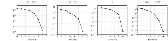
Figure 4: Convergence behavior of 10224-bus system by applying reduced modeling method with the Gauss-Newton based inexact aladin algorithm

TABLE III: Computing time for solving power flow problem with different combinations

			Original model			Reduced model
Buses			Dimension	standard[s]	inexact[s]	Dimension	standard[s]	inexact[s]	centralized
53	3	5	232	0.143	0.027	126	0.114	0.011	0.004
418	2	8	1704	0.485	0.068	868	0.315	0.028	0.014
2708	2	30	10952	3.913	0.236	5536	2.149	0.109	0.051
4662	5	130	19168	10.442	0.451	9844	5.694	0.228	0.129
10224	13	242	41864	25.909	0.996	21416	14.392	0.591	0.257

VI Conclusions

The present paper investigates the application of a new tailored version of aladin for solving the ac power flow (pf)problem. Compared with the previous work by Mühlpfordt et al. (2021), the dimension by applying reduced modelling method can be reduced by half. By applying the Gauss-Newton based inexact aladin, we trade off the convergence rate slightly for the great improvement on computing time. Besides, no external nlp solver is needed. In general, this new combination is of great potential for handling large-scale systems, and turns out to be as efficient as a centralized approach. For future work, efforts toward parallel computing will be made to reduce the computing time even further.

References

- Grainger (1999) J. J. Grainger, Power system analysis. McGraw-Hill, 1999.
- Mühlpfordt et al. (2021) T. Mühlpfordt, X. Dai, A. Engelmann, and V. Hagenmeyer, “Distributed power flow and distributed optimization—formulation, solution, and open source implementation,” Sustainable Energy, Grids and Networks, vol. 26, p. 100471, 2021.
- Hug-Glanzmann and Andersson (2009) G. Hug-Glanzmann and G. Andersson, “Decentralized optimal power flow control for overlapping areas in power systems,” IEEE Transactions on Power Systems, vol. 24, no. 1, pp. 327–336, 2009.
- Baldick et al. (1999) R. Baldick, B. H. Kim, C. Chase, and Y. Luo, “A fast distributed implementation of optimal power flow,” IEEE Transactions on Power Systems, vol. 14, no. 3, pp. 858–864, 1999.
- Erseghe (2014) T. Erseghe, “Distributed optimal power flow using ADMM,” IEEE transactions on power systems, vol. 29, no. 5, pp. 2370–2380, 2014.
- Kim and Baldick (2000) B. H. Kim and R. Baldick, “A comparison of distributed optimal power flow algorithms,” IEEE Transactions on Power Systems, vol. 15, no. 2, pp. 599–604, 2000.
- Guo et al. (2016) J. Guo, G. Hug, and O. K. Tonguz, “A case for nonconvex distributed optimization in large-scale power systems,” IEEE Transactions on Power Systems, vol. 32, no. 5, pp. 3842–3851, 2016.
- Sun and Sun (2021) K. Sun and X. A. Sun, “A two-level ADMM algorithm for AC OPF with convergence guarantees,” IEEE Transactions on Power Systems, 2021.
- Houska et al. (2016) B. Houska, J. Frasch, and M. Diehl, “An augmented Lagrangian based algorithm for distributed nonconvex optimization,” SIAM Journal on Optimization, vol. 26, no. 2, pp. 1101–1127, 2016.
- Engelmann et al. (2018) A. Engelmann, Y. Jiang, T. Mühlpfordt, B. Houska, and T. Faulwasser, “Toward distributed OPF using ALADIN,” IEEE Transactions on Power Systems, vol. 34, no. 1, pp. 584–594, 2018.
- Meyer-Huebner et al. (2019) N. Meyer-Huebner, M. Suriyah, and T. Leibfried, “Distributed optimal power flow in hybrid AC–DC grids,” IEEE Transactions on Power Systems, vol. 34, no. 4, pp. 2937–2946, 2019.
- Du et al. (2019) X. Du, A. Engelmann, Y. Jiang, T. Faulwasser, and B. Houska, “Distributed state estimation for AC power systems using Gauss-Newton ALADIN,” in 2019 IEEE 58th Conference on Decision and Control (CDC). IEEE, 2019, pp. 1919–1924.
- Engelmann et al. (2020) A. Engelmann, Y. Jiang, H. Benner, R. Ou, B. Houska, and T. Faulwasser, “ALADIN-—an open-source matlab toolbox for distributed non-convex optimization,” Optimal Control Applications and Methods, 2020.
- Frank and Rebennack (2016) S. Frank and S. Rebennack, “An introduction to optimal power flow: Theory, formulation, and examples,” IIE transactions, vol. 48, no. 12, pp. 1172–1197, 2016.
- Nocedal and Wright (2006) J. Nocedal and S. Wright, Numerical optimization. Springer Science & Business Media, 2006.
- Andersson et al. (2019) J. A. Andersson, J. Gillis, G. Horn, J. B. Rawlings, and M. Diehl, “Casadi: a software framework for nonlinear optimization and optimal control,” Math. Program. Comput.”, vol. 11, no. 1, pp. 1–36, 2019.
- Wächter and Biegler (2006) A. Wächter and L. T. Biegler, “On the implementation of an interior-point filter line-search algorithm for large-scale nonlinear programming,” Math. Program., vol. 106, no. 1, pp. 25–57, 2006.
- Zimmerman et al. (2010) R. D. Zimmerman, C. E. Murillo-Sánchez, and R. J. Thomas, “Matpower: Steady-state operations, planning, and analysis tools for power systems research and education,” IEEE Trans. Power Syst., vol. 26, no. 1, pp. 12–19, 2010.