Instantaneous Frequency Estimation In Multi-Component Signals Using Stochastic EM Algorithm

Abstract

This paper addresses the problem of estimating the modes of an observed non-stationary mixture signal in the presence of an arbitrary distributed noise. A novel Bayesian model is introduced to estimate the model parameters from the spectrogram of the observed signal, by resorting to the stochastic version of the EM algorithm to avoid the computationally expensive joint parameters estimation from the posterior distribution. The proposed method is assessed through comparative experiments with state-of-the-art methods. The obtained results validate the proposed approach by highlighting an improvement of the modes estimation performance.

1 Introduction

In this work, we introduce a novel observation model for estimating the instantaneous frequency of modes of Multicomponent Signal (MCS) in the presence of an arbitrary distributed noise. For this purpose, we use the signal spectrogram defined as the squared modulus of the Short-Time Fourier Transform (STFT), and consider the 1D signals observed by selecting a given time instant of the spectrogram. While performing parameters estimation using classical algorithms such as [14] is challenging in the presence of noise, more methods assuming the presence of spurious content [8, 9, 1, 2] achieve satisfactory estimation performance until average to low Signal-to-Noise Ratio (SNR). However these methods are generally made to deal with the presence of Gaussian noise and do not address the estimation problem in more complex scenarios (Poisson or gamma noise, mixture of noise). Here, we develop a method in a Bayesian framework for estimating the modes Instantaneous Frequency (IF) where a mixture model is used to account for the presence of both the signal components and an arbitrary distributed noise. Prior models are associated with the parameters to model the available a priori knowledge. An adapted estimation strategy is then formulated through a Stochastic Expectation-Maximization (SEM) algorithm [12, 3] to avoid intractable joint parameters estimation from the posterior distribution and to deal with the Markovian nature of the prior models. This paper is organized as follows. In Section 2 we introduce the observation model and the prior distributions associated with the model parameters. We then discuss the estimation strategy in Section 3, and comparatively evaluate the performance of the proposed method in Section 4 with numerical results. Conclusions and future work are finally reported in Section 5.

2 Observation model

Let $x$ be a mixture made of $K$ superimposed Amplitude-and Frequency-Modulated (AM-FM) components expressed as:

$$x(n)=\sum_{k=1}^{K}x^{k}(n)\text{,\quad with }x^{k}(n)=a^{k}(n)\,\mathbf{e}^{j\phi^{k}(n)},$$ (1)

where $a^{k}(n)$ and $\phi^{k}(n)$ are respectively the time-varying amplitude and angular phase of the $k$th component at time $n$. The discrete-time STFT of a signal $x$, using an analysis window $\theta$ s.t. $\theta(n)=\frac{1}{\sqrt{2\pi}L}\,\mathbf{e}^{-\frac{n^{2}}{2L^{2}}}$, with $L$ being the time spread parameter, can be defined at each time instant $n\in[0,N-1]$ and each frequency bin $m\in[0,M-1]$, as:

$$F^{\theta}_{x}(n,m)=\displaystyle\sum_{l=-\infty}^{+\infty}x(l)\theta(n-l)^{*}\,\mathbf{e}^{-j\frac{2\pi lm}{M}},$$ (2)

with $z^{*}$ the complex conjugate of $z$. Let $\boldsymbol{S}=\{|F_{x}^{\theta}|^{2}\}_{n,m}$ be the spectrogram of $x$. We denote the $\mathds{R}^{M\times 1}$ spectrogram columns as $\boldsymbol{s}_{n}=[s_{n,0},\ldots,s_{n,M-1}]^{\top}$, with $\boldsymbol{S}=\{\boldsymbol{s}_{n}\}_{n=1}^{N}$. In this work, we are interested in estimating the ridge positions $\boldsymbol{\hat{m}}_{n}=[\hat{m}_{n}^{1},\dots,\hat{m}_{n}^{K}]^{\top}$ associated with the IF $\boldsymbol{\phi}^{\prime}_{n}=\{\frac{d\phi^{k}}{dn}(n)\}_{k=1}^{K}$, $\forall n\in[0,N-1]$. For that purpose, we assume the following observation model:

$$p(s_{n,m}|\boldsymbol{w}_{n},\boldsymbol{\hat{m}}_{n})=\sum_{k=1}^{K}w_{n}^{k}g(m-\hat{m}_{n}^{k})+\frac{1}{M}\left(1-\sum_{k=1}^{K}w_{n}^{k}\right),$$ (3)

where $g(m)=\frac{2\sqrt{\pi}L}{M}\,\mathbf{e}^{-\left(\frac{2\pi mL}{M}\right)^{2}}$ is the normalized and discretized squared modulus of the Fourier transform of $\theta$, such that (s.t.) the integral of $g$ remains constant over the admissible values of $\boldsymbol{\hat{m}}_{n}$. In (3), the weight $w_{n}^{k}$ represents the probability of each element of $\boldsymbol{s}_{n}$ to belong to the $k$th component s.t. $w_{n,k}=\frac{a_{n}^{k}}{\sum_{k=1}^{K}a_{n}^{k}+Mb_{n}}$, with $b_{n}$ the average noise amplitude at time $n$. Conversely, $(1-\sum_{k=1}^{K}w_{n}^{k})$ is the probability to observe noise in $\boldsymbol{s}_{n}$. Note that the weights $\boldsymbol{w}_{n}=[w_{n}^{1},\ldots,w_{n}^{K}]^{\top}$ are constrained to belong to $[0,1]^{K}$ s.t. $\sum_{k}w_{n}^{k}\leq 1$. For further development, we set $\boldsymbol{W}=\{\boldsymbol{w}_{n}\}_{n=0}^{N-1}$ and $\boldsymbol{\hat{\mathcal{M}}}=\{\boldsymbol{\hat{m}}_{n}\}_{n=0}^{N-1}$. Assuming independence between each Time-Frequency (TF) instant conditioned on the value of $(\boldsymbol{w}_{n},\boldsymbol{\hat{m}}_{n})$, we express the joint likelihood function as

$$p(\boldsymbol{S}|\boldsymbol{W},\boldsymbol{\hat{\mathcal{M}}})=\prod_{n}\prod_{m}p(s_{n,m}|\boldsymbol{w}_{n},\boldsymbol{\hat{m}}_{n}).$$ (4)

In order to complete the Bayesian model, prior distributions have to be assigned to the model parameters to account for the a priori available knowledge [7]. First, a weak uniform prior model is associated with the elements of $\boldsymbol{W}$.

Total Variation In the presence of strong noise (low SNR), the ridges in the TF plane can be split or partially destroyed. It can thus be preferable for the IF estimates to not significantly move away from the estimation performed in the TF area with strong local maxima. We thus define the following Total Variation (TV) Markov Random Field (MRF) prior model for $\boldsymbol{\hat{\mathcal{M}}}$ which preserves sharp edges [4, 15]

$$p(\boldsymbol{\hat{\mathcal{M}}}|\epsilon)\propto\exp\left[-\epsilon\sum_{k=1}^{K}\|\boldsymbol{\hat{m}}_{k,:}^{\top}\|_{TV}\right],$$ (5)

with $\boldsymbol{\hat{m}}_{k,:}$ the $k$th row of $\boldsymbol{\hat{\mathcal{M}}}$, $\epsilon$ a fixed user-defined hyper-parameter and $\|x\|_{TV}$ the sum of the absolute values of the partial derivatives of $x$.

Laplacian Another possible choice for regularizing $\boldsymbol{\hat{\mathcal{M}}}$ is to constrain the mean curvature of the estimated ridge, remaining to bound the IF second derivatives. This is performed using a MRF Laplacian prior model [16, 13] by setting a $\ell_{2}$-norm penalization on the curvature of $\boldsymbol{\hat{\mathcal{M}}}$ as

$$p(\boldsymbol{\hat{\mathcal{M}}}|\lambda)\propto\exp\left[-\frac{\lambda}{2}\sum_{k=1}^{K}\|\boldsymbol{L}_{a}\boldsymbol{\hat{m}}_{k,:}^{\top}\|_{2}^{2}\right],$$ (6)

where $\boldsymbol{L}_{a}$ is the log-concave and differentiable Laplacian operator, s.t. $\|\boldsymbol{L}_{a}x\|_{2}^{2}$ is the sum of the squared partial derivatives of $x$. This operator controls the smoothness of the estimation. Similarly to the TV prior model, we assume $\lambda$ to be a fixed hyperparameter.

3 Estimation strategy

For the sake of clarity, we omit in the sequel the priors related hyper-parameters $\epsilon$ and $\lambda$ from the equations. Using Bayes rule, the joint posterior distribution of $(\boldsymbol{w},\boldsymbol{\hat{\mathcal{M}}})$ can be approximated as

$$p(\boldsymbol{W},\boldsymbol{\hat{\mathcal{M}}}|\boldsymbol{S})\propto p(\boldsymbol{S}|\boldsymbol{W},\boldsymbol{\hat{\mathcal{M}}})p(\boldsymbol{\hat{\mathcal{M}}})p(\boldsymbol{W}).$$ (7)

Estimating jointly $(\boldsymbol{W},\boldsymbol{\hat{\mathcal{M}}})$ is challenging due to the shape of the likelihood in Eq. (4) being multimodal with respect to $\boldsymbol{\hat{\mathcal{M}}}$. Thus, we propose to marginalize over the hidden parameter $\boldsymbol{\hat{\mathcal{M}}}$ to perform the estimation of $\boldsymbol{W}$ as the Marginal Maximum a Posteriori (MMAP) estimation as follow

$$\widehat{\boldsymbol{W}}_{\text{MMAP}}=\underset{\boldsymbol{W}}{\textrm{argmax}}~{}~{}p(\boldsymbol{W}|\boldsymbol{S}).$$ (8)

Expectation-Maximization (EM)-based algorithms are particularly adapted to address this problem. Moreover, the shape of the model in Eq. (3) is well suited to apply such methods. It remains to compute $p(\boldsymbol{W}|\boldsymbol{S})=\sum_{\boldsymbol{\hat{\mathcal{M}}}}p(\boldsymbol{W},\boldsymbol{\hat{\mathcal{M}}}|\boldsymbol{S})$, before solving Eq. (8) in a second time.

3.1 Estimation of mixture weights

Given $\boldsymbol{W}^{(i)}$ the current estimation of $\boldsymbol{W}$ at iteration $i$, the E-step is given at each iteration by

$$Q(\boldsymbol{W}|\boldsymbol{W}^{(i)})=E_{\boldsymbol{\hat{\mathcal{M}}}|\boldsymbol{S},\boldsymbol{W}^{(i)}}\left[\log(p(\boldsymbol{S},\boldsymbol{\hat{\mathcal{M}}}|\boldsymbol{W}))\right].$$ (9)

While classical EM-based algorithms are well adapted to solve problems involving hidden parameters, performing the M-step is computationally intractable due to the Markovian nature of the prior models introduced in Eq. (5)-(6). We thus resort to the SEM [12, 3, 10] s.t. $p(\boldsymbol{\hat{\mathcal{M}}}|\boldsymbol{W}^{(i)},\boldsymbol{S})$ in Eq. (9) approximated using Markov chain Monte Carlo (MCMC) simulations. More precisely, we simulate $N_{s}$ samples $\{\boldsymbol{\bar{\mathcal{M}}}_{1},\ldots,\boldsymbol{\bar{\mathcal{M}}}_{N_{s}}\}$ from $p(\boldsymbol{\hat{\mathcal{M}}})$ using a 2-step Gibbs sampler as

$$\boldsymbol{\bar{m}}_{n}=\underset{\boldsymbol{\hat{m}}_{n}}{\textrm{argmax}}\sum_{l=0,l\neq n}^{N-1}p(\boldsymbol{\hat{m}}_{n}|\boldsymbol{\hat{m}}_{l}),$$ (10)

with $\boldsymbol{\bar{\mathcal{M}}}=\{\boldsymbol{\bar{m}}_{n}\}_{n=0}^{N-1}$. These samples are then used as an approximation of $p(\boldsymbol{\hat{\mathcal{M}}})$ and Bayes rule is applied to compute an approximate distribution $\tilde{p}(\boldsymbol{\hat{\mathcal{M}}}|\boldsymbol{W}^{(i)},\boldsymbol{S})$. We finally compute a current estimation $\boldsymbol{\widetilde{\mathcal{M}}}$ of $\boldsymbol{\hat{\mathcal{M}}}$ from $\tilde{p}(\boldsymbol{\hat{\mathcal{M}}}|\boldsymbol{W}^{(i)},\boldsymbol{S})$ using a sequential MMAP estimation which will be discussed in Section 3.2. The convergence speed of the algorithm is increased by hot-starting the Gibbs sampler at each iteration using the previously generated samples. The two main steps of the EM algorithm become

$$\begin{split}\widehat{Q}(\boldsymbol{W}|\boldsymbol{W}^{(i)})&=\log p(\boldsymbol{S}|\boldsymbol{W},\boldsymbol{\widetilde{\mathcal{M}}})+\log\left[p(\boldsymbol{\hat{\mathcal{M}}})p(\boldsymbol{W})\right],\\ \boldsymbol{W}^{(i+1)}&=\underset{\boldsymbol{W}}{\textrm{argmax}}~{}~{}\widehat{Q}(\boldsymbol{W}|\boldsymbol{W}^{(i)}).\end{split}$$ (11)

The concavity of the likelihood in Eq. (3) with respect to $\boldsymbol{W}$ ensures that of $\widetilde{Q}(\boldsymbol{W}|\boldsymbol{W}^{(i)})$, allowing the use of convex optimization approaches to solve the M-step in Eq. 11. Maximization is thus performed using a Newton-Raphson second-order gradient ascent algorithm to update $\boldsymbol{W}$. We set the same EM algorithm stopping criterion as in [11].

3.2 Instantaneous frequency estimation

Although having marginalized over the nuisance variable to estimate $\boldsymbol{W}$ allows to significantly reduce the computational cost of the whole estimation process, the approximate posterior in Eq. (10) remains non convex due to the presence of multiple components. Here, we estimate $\boldsymbol{\widetilde{\mathcal{M}}}$ by iteratively performing MMAP estimation from $p(\boldsymbol{\hat{\mathcal{M}}}|\boldsymbol{\widetilde{W}},\boldsymbol{S})$, before discarding the estimate neighborhood in the posterior distribution, until $K$ estimates have been computed. Even though discarding $3$ times the standard deviation $\sigma_{d}=\sqrt{M/(\pi L)}$ of the data distribution would be a good choice (three-sigma rule of thumb), the presence of slightly frequency modulated components [5] avoided proper discard of the information related to the last MMAP estimate. We thus consider a slightly broader window by considering $3\sigma_{d}+1$, rounded up. Note that this choice depends on the frequency resolution of the STFT.

4 Results

In this section, we assess the IF estimation performance of the proposed approach on a MCS in the presence of additive noise. The MCS depicted in Fig. 1 is made of two linear chirps overlapping at time index $225$.

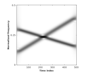
Figure 1: Spectrogram of the analyzed multicomponent signals with overlapping components.

For the experiments conducted in this section, we compute the STFT using the ASTRES toolbox [6], with $N=500$ and $L=20$. Moreover, an additive white Gaussian noise controlled through a SNR varying from -20 to 20 dB, is added to the MCS in order to model the presence of a spurious content. For comparison purpose, we select the pseudo-Bayesian (PB) approach proposed in [9], both the simple and spline Ridge Detector (RD) of [8] and the Brevdo method [1]. For the latter we keep the same hyperparameter values than that presented in [1]. For the proposed method, we set $\epsilon=10^{-3},\lambda=10^{-2}$ since it provides the best performances during our experiments. Note however that those values have to be defined according to the TF resolution. For each method, we reconstruct the signals by selecting at each time instant in the Time-Frequency Representation (TFR), a neighborhood of $2\times 3\sigma_{d}+1$ frequency values centered around the estimated IF of each component. This ensures most of the ridges information to be encapsulated in informative ribbons. A hard threshold is then applied on the TFR and the TF instants outside of the ribbons are set to zeros value. The inverse STFT is finally applied on the hard thresholded TFR in order to compare the estimated signal to its ground truth. The estimation performance of the method is thus assessed using the Reconstruction Quality Factor (RQF): $10\log_{10}\left(\frac{||x||^{2}}{||x-\hat{x}||^{2}}\right)$ where $x$ (resp. $\hat{x}$) stands for the reference (resp. estimated) signal.

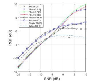
Figure 2: RQF of the first ridge with increasing frequency depicted in Fig. 1 obtained with the competing methods (averaged over 50 realizations of noise) for a varying SNR.

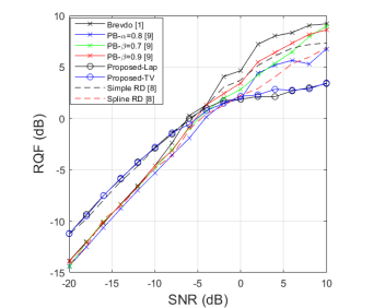
Figure 3: RQF of the second ridge with decreasing frequency depicted in Fig. 1 obtained with the competing methods (averaged over 50 realizations of noise) for a varying SNR.

From Fig. 2 and Fig. 3, we observe that the proposed approach using both prior models outperforms other at low SNR. The performance of the proposed method remains nonetheless similar to that of the spline RD [8] in Fig. 3. Note that the experiment, and more particularly the reconstruction of the TFR using a hard threshold, is not adapted to high SNR cases since we mostly discard informative content. The RQF is however adapted for low SNR scenarios, even though the TF content surrounding the estimated IF used to reconstruct the signals is also contaminated by noise. Both the TV and Laplacian prior models in the proposed approach provide similar performance, even though the TV prior perform better at high SNR (see Fig. 3).

5 Conclusion

In this work, we introduced a new observation model to perform estimation of the IF of a signal component in the presence of an arbitrary distributed noise. The presence of spurious content is approximated as a uniform distribution to allow the modelling of any additive noise. The model formulation is well suited for inference using EM algorithms, allowing to reduce the problem complexity and to estimate the mixture weights with a low computational time. The stochastic approach significantly lightens the computation of the E-step when using Markovian prior models. A sequential MMAP estimation is performed to account for the multimodal nature of the IF posterior distribution, even in scenarios involving overlapping ridges. The results demonstrate the ability of the proposed inference method to outperform the competing approaches in the low SNR regime. Future work include an estimation of the modulation rate [5] by extending, for instance, the method into a generalized EM [12]. A more general estimation process accounting for the estimation of the hyperparameters is currently under investigation.

References

- [1] E. Brevdo, N. S. Fuckar, G. Thakur, and H-T. Wu. The synchrosqueezing algorithm: a robust analysis tool for signals with time-varying spectrum. Computing Research Repository - CORR, 01 2011.
- [2] Rene Carmona, Wen Hwang, and Bruno Torrésani. Characterization of signals by the ridges of their wavelet transforms. IEEE Trans. Signal Process., 45:2586–2590, 01 1997.
- [3] G. Celeux, D. Chauveau, and J. Diebolt. Stochastic versions of the EM algorithm: an experimental study in the mixture case. Journal of Stat. Comp. and Simulation, 55(4):287–314, 1996.
- [4] A. Chambolle. An algorithm for total variation minimization and applications. Journal of Mathematical imaging and vision, 20(1):89–97, 2004.
- [5] M. Colominas, S. Meignen, and D. H. Pham. Time-frequency filtering based on model fitting in the time-frequency plane. IEEE Signal Processing Lett., PP:1–1, 03 2019.
- [6] D. Fourer, J. Harmouche, J. Schmitt, T. Oberlin, S. Meignen, F. Auger, and P. Flandrin. The ASTRES toolbox for mode extraction of non-stationary multicomponent signals. In Proc. EUSIPCO, pages 1130–1134, Aug. 2017.
- [7] D. Iatsenko, P.V.E. McClintock, and A. Stefanovska. Extraction of instantaneous frequencies from ridges in time–frequency representations of signals. Signal Processing, 125:290–303, 2016.
- [8] N. Laurent and S. Meignen. A novel ridge detector for nonstationary multicomponent signals: Development and application to robust mode retrieval. IEEE Trans. Signal Process., 69:3325–3336, 2021.
- [9] Q. Legros and D. Fourer. A novel pseudo-Bayesian approach for robust multi-ridge detection and mode retrieval. In Proc. EUSIPCO, Aug. 2021.
- [10] Q. Legros, S. McLaughlin, Y. Altmann, and S. Meignen. Stochastic EM algorithm for fast analysis of single waveform multi-spectral Lidar data. In Proc. EUSIPCO, pages 2413–2417, 2021.
- [11] Q. Legros, S. Meignen, S. McLaughlin, and Y. Altmann. Expectation-Maximization based approach to 3D reconstruction from single-waveform multispectral Lidar data. IEEE Trans. Comput. Imaging, 2020.
- [12] G. McLachlan and T. Krishnan. The EM algorithm and extensions, volume 382. John Wiley & Sons, 2007.
- [13] M. Meyer, M. Desbrun, P. Schroder, and A. H. Barr. Discrete differential-geometry operators for triangulated 2-manifolds. In Visualization and Math. III, pages 35–57. Springer Berlin Heidelberg, 2003.
- [14] G. Rilling and P. Flandrin. One or two frequencies? The empirical mode decomposition answers. IEEE Trans. Signal Process., 56(1):85–95, 2007.
- [15] L. I. Rudin, S. Osher, and E. Fatemi. Nonlinear total variation based noise removal algorithms. Physica D: nonlinear phenomena, 60(1-4):259–268, 1992.
- [16] X. Wang. Laplacian operator-based edge detectors. IEEE Trans. Patt. Anal. Mach. Intell., 29:886–90, June 2007.