FlexFringe: Modeling Software Behavior by Learning Probabilistic Automata

Abstract.

We present the efficient implementations of probabilistic deterministic finite automaton learning methods available in FlexFringe. These implement well-known strategies for state-merging including several modifications to improve their performance in practice. We show experimentally that these algorithms obtain competitive results and significant improvements over a default implementation. We also demonstrate how to use FlexFringe to learn interpretable models from software logs and use these for anomaly detection. Although less interpretable, we show that learning smaller more convoluted models improves the performance of FlexFringe on anomaly detection, outperforming an existing solution based on neural nets.

1. Introduction

We present the probabilistic deterministic finite state automaton (PDFA) learning methods implemented in the open source FlexFringe automaton learning package and demonstrate how to use them when dealing with software data. In previous work [VH17], the value of learning non-probabilistic automata for bug discovery was demonstrated. It is often easier to learn probabilistic automata since these do not require labeled data. In this paper, we describe the inner workings of the probabilistic learning methods in FlexFringe and show how they can be used to detect behavioral anomalies in a software system. Furthermore, we show how to analyze the discovered anomalous patterns. Our main goal is to get a wider audience interested in the efficient state-merging methods implemented in FlexFringe. We therefore highlight the flexible and interpretable nature of FlexFringe, as well as its efficiency and practical performance. This document can be used as a guide on developing extensions in FlexFringe or other new state-merging methods.

FlexFringe originated from the DFASAT [HV10] algorithm for learning non-probabilistic deterministic finite automata (DFA) and is based on the well-known red-blue state merging framework [LPP98]. Learning automata from trace data [CW98] has been used for analyzing different types of complex software systems such as web-services [BIPT09, ISBF07], X11 programs [ABL02], communication protocols [CWKK09, ANV11, FBLP⁺17, FBJM⁺20], Java programs [CBP⁺11], and malicious software [CKW07, CKW07]. A great benefit that state machines provide over more traditional machine learning models is that software systems are in essence state machines. Hence, these models give unparalleled insight into the inner workings of software and can even be used as input to software testing techniques [LY96].

Learning state machines from traces can be seen as a grammatical inference [DlH10] problem where traces are modeled as the words of a language, and the goal is to find a model for this language, e.g., a (probabilistic) deterministic finite state automaton [HMU01]. Although the problem of learning a (P)DFA is NP-hard [Gol78] and hard to approximate [PW93], state merging is an effective heuristic method for solving this problem [LPP98]. This method starts with a large tree-shaped model, called the prefix tree, that directly encodes the input traces. It then iteratively combines states by testing the similarity of their future behaviours using a Markov property [NN98] or a Myhill-Nerode congruence [HMU01]. This process continues until no similar states can be found. The result is a small model displaying the system states and transition structure hidden in the data. Figure 1 shows the prefix tree for a small example data set consisting of 20 sequences starting with an “a” event and ending in a “b” event. Running FlexFringe results in the PDFA shown in Figure 2.

Figure 1. A prefix tree printed by FlexFringe and displayed using Graphviz dot. Each state contains occurrence counters for the total number of traces, as well as how many of them end (fin counts) or pass through (path counts) for each trace type. You can use these to infer what traces occurred in the training data, e.g., a-a-a-b-b occurred 3 times, following transitions from state 0-1-2-4-9 and ending in state 17. The transitions are labeled by symbols and occurrence counts. The initial state has a solid edge, indicating it has already been learned as an automaton state. The dotted states can still be merged with both solid and dotted states.

Figure 2. A PDFA printed after running FlexFringe. It contains the same type of counts as the prefix tree. To obtain a PDFA from these counts, one simply needs to normalize them. Traces only end in the third state, as indicated by the fin counts. The learned PDFA correctly represents the set of traces starting with “a” and ending in “b”, i.e., $a(a|b)^{*}b$. A learned PDFA can be used for assigning probabilities to new sequences by following transitions and multiplying their probabilities. It can also be used for anomaly detection, for instance by checking whether a new trace ends in a state with fin counts greater than 0 (a final state).

The key design principle of FlexFringe is that this state merging approach can be used to learn models for a wide range of systems, including Mealy and I/O machines [SG09, AV10], probabilistic deterministic automata [VTDLH⁺05, VEDLH14], timed/extended automata [Ver10, NSV⁺12, NSV⁺12, SK14, WTD16], and regression automata [LHPV16]. All that needs to be modified is the similarity test, implemented as an evaluation function that tests for merge consistency and computes a score function to decide between possible consistent merges. In FlexFringe, these functions can be implemented and modified by adding only a single file (the evaluation function) to the code base. This file needs to implement:

• methods for processing evaluation function specific inputs such as time values,

• data structures that contain information such as frequency counts,

• methods that compute merge consistency and merge score from these structures,

• and updating routines for modifying their content due to a performed merge.

These functions can be derived and overloaded from existing evaluation functions. FlexFringe then provides efficient state-merging routines that determine which merge to perform, how this influences the automaton structure, and different ways to prioritize and search through the possible merges. This process can be fine-tuned using several parameters.

With FlexFringe, we aim to make efficient state-merging algorithms accessible to a wide range of users. Currently, most users are from the software engineering domain because they frequently deal with data generated by deterministic systems. In practice, data is usually unlabeled since one can only observe what a (software) system does and not what it does not do. Most applications of state merging therefore make use of some form of PDFA learning. We have implemented several evaluation functions in FlexFringe for well-known PDFA learning algorithms such as Alergia [CO94], MDI [Tho00], Likelihood-ratio [VWW10], and AIC minimization [Ver10]. In this paper, we describe these methods and improvements we developed to boost their performance in practice:

• We show the inner workings of efficient implementations for state-merging algorithms.

• We provide improvements over the traditional implementations that increase performance in practice.

• We perform experiments on the PAutomaC data set [VEDLH14] displaying competitive results.

• For a use-case on software logs from the HDFS data set [XHF⁺09], we demonstrate how to learn insightful models and outperform existing solutions based on neural nets.

This paper is organized as follows. We start with an overview of PDFAs and the state-merging algorithm in Sections 2 and 3, including a description of the efficient data structures used in FlexFringe. We then describe the implemented PDFA evaluation functions in Section 4 and the developed improvements in Section 5. The results obtained using the different evaluation functions on the PAutomaC competition data sets are discussed in Section 7. For software log data, we show the performance on the HDFS data from both insight and performance perspectives in Section 8. We provide an overview of closely related algorithms and tools in Section 9, and end with some concluding remarks in Section 10.

2. Probabilistic Automata

Automata or state machines are models for sequential behavior. Like hidden Markov models, they are models with hidden/latent state information. Given a string (trace) of observed symbols (events) $a_{1},\ldots,a_{n}$, this means that the corresponding system states $q_{0},q_{1},\ldots,q_{n}$ are unknown/unobserved. In deterministic automata, we assume that there exists a unique start state $q_{0}$ and that there are no unobserved events (no $\epsilon$-transitions). Furthermore, given the current system state $q_{i}$ and the next event $a_{i+1}$ there is a unique next state $q_{i+1}$. This implies that deterministic automata can be in exactly one state at every time step. Although hidden Markov models do not have this restriction, it is well-known that automata can be transformed into hidden Markov models and vice versa [DDE05]. Determinism can be important when modeling sequential behavior because the resulting models are frequently easier to interpret. Moreover, the computation of state sequences and probabilities is much more efficient.

A probabilistic deterministic finite state automaton (PDFA) is a tuple $\mathcal{A}=\{\Sigma,Q,q_{0},\delta,S,F\}$, where $\Sigma$ is a finite alphabet, $Q$ is a finite set of states, $q_{0}\in Q$ is a unique start state, $\delta:Q\times\Sigma\to Q\cup\{0\}$ is the transition function, $S:Q\times\Sigma\to\left[0,1\right]$ is the symbol probability function, and $F:Q\to\left[0,1\right]$ is the final probability function, such that $F(q)+\sum_{a\in\Sigma}S(q,a)=1$ for all $q\in Q$.

Given a sequence of observed symbols $s=a_{1},\ldots,a_{n}$, a PDFA $\mathcal{A}$ can be used as a function to assign/compute probabilities $\mathcal{A}(s)=S(q_{0},a_{1})\cdot S(q_{1},a_{2})\ldots S(q_{n-1},a_{n})F(q_{n})$, where $\delta(q_{i},a_{i+1})=q_{i+1}$ for all $0\leq i\leq n-1$. A probabilistic automaton is deterministic when its transition function $\delta$ (and hence its structure) is deterministic, meaning that for each state $q\in Q$ and symbol $s\in\Sigma$, $\delta(q,s)$ maps to exactly one state. In a non-deterministic automaton, this function maps to a subset of $Q$. The transition function is extended with a null symbol ($0$), representing that the transition does not exist. We thus allow PDFA models to be incomplete. A PDFA computes a probability distribution over $\Sigma^{*}$, i.e., $\sum_{s\in\Sigma^{*}}\mathcal{A}(s)=1$. A PDFA can also be defined without final probability function $F$, in that case it computes probability functions over $\Sigma^{n}$, i.e., $\sum_{s\in\Sigma^{n}}\mathcal{A}(s)=1$ for all $1\leq n$.

PDFAs are excellent models for systems that display deterministic behavior such as software. PDFAs and their extensions have frequently been used to model tasks in both software and cyber-physical systems, see, e.g., [NVMY21, KABP14, WRSL21, HMS⁺16] and [LVD20, SK14, LAVM18, Mai14, PLHV17]. In addition to their ability to compute probabilities and predict future symbols, their deterministic nature provides insight into a system’s inner working and can even be used to fully reverse engineer a system from observations [ANV11].

3. State merging in FlexFringe

Given a finite data set of example sequences $D$ called the input sample, the goal of PDFA learning (or identification) is to find a (non-unique) small PDFA $\mathit{A}$ that is consistent with $D$. We call such sequences positive or unlabeled. In contrast, DFAs are commonly learned from labeled data containing both positive and negative sequences. PDFA size is typically measured by the number of states ($|Q|$) or transitions ($|\{(q,a)\in Q\times\Sigma:\delta(q,a)\not=0\}|$).

Consistency is tricky to define when dealing with only positive data. Most methods define consistency by putting restrictions on the merge steps performed by the algorithm. Intuitively, a merge step concludes that for two states $q$ and $q^{\prime}$, the future sequences in $D$ occurring after reaching $q$ or $q^{\prime}$ are similarly distributed. Since $q$ and $q^{\prime}$ can be reached by different past sequences, this boils down to a type of test for a Markov property: the future is independent from the past given the current state, i.e., $\frac{\mathcal{A}(s_{q}z)}{\mathcal{A}(s_{q})}\approx\frac{\mathcal{A}(s_{q^{\prime}}z)}{\mathcal{A}(s_{q^{\prime}})}$ for all suffixes $z\in\Sigma^{*}$, where $s_{q}$ and $s_{q}^{\prime}$ are prefixes ending in state $q$ and $q^{\prime}$, respectively. States in a PDFA can thus be thought of as clusters of prefixes with similarly distributed suffixes. In addition, the restriction of using a deterministic model requires that if $s_{q}$ and $s_{q^{\prime}}$ are clustered, then $s_{q}z$ and $s_{q^{\prime}}z$ are clustered as well for all $z\in\Sigma^{*}$, called the determinization constraint, i.e., $\frac{\mathcal{A}(s_{q}yz)}{\mathcal{A}(s_{q}y)}\approx\frac{\mathcal{A}(s_{q^{\prime}}yz)}{\mathcal{A}(s_{q^{\prime}}y)}$ for all suffixes $y,z\in\Sigma^{*}$. During the learning process, we of course do not know $\mathcal{A}$ but can estimate it using the partially constructed model that is being learned.

Finding a small and consistent PDFA is a well-known hard problem and an active research topic in the grammatical inference community, see, e.g. [DlH10]. One of the most successful state merging approaches for finding a small and consistent (P)DFA is evidence-driven state-merging in the red-blue framework (EDSM) [LPP98]. FlexFringe implements this framework making use of union/find structures to keep track of performed merges and efficiently undo them, see Figure 3. Like most state merging methods, FlexFringe first constructs a tree-shaped PDFA $\mathit{A}$ known as a prefix tree from the input sample $D$, see Figure 1. Afterwards, it iteratively merges the states of $\mathit{A}$. Initially, since every prefix leads to a unique state, $\mathit{A}$ is consistent with $D$. A merge (see Algorithm 1 and Figures 3 and 4 to compare models before and after merging state 2 with state 1) of two states $q$ and $q^{\prime}$ combines the states into one by setting the representative variable from the union/find structure of $q^{\prime}$ to $q$. After this merge, whenever a computation of a sequence returns $q^{\prime}$, it returns the representative $q$ instead of $q^{\prime}$. A merge is only allowed if the states are consistent, determined using a statistical test or distance computation based on their future sequences. A unique feature of FlexFringe is that users of the algorithm are able to implement their own test by adding a single file called the evaluation function to the source code. It is even possible to add additional attributes such as continuous sensor reading to input symbols and use these in a statistical test to learn regression automata [LHPV16].

Figure 3. The union/find data structure in FlexFringe after performing the first merge operation (state 2, reached by a-a, is merged with state 1, creating a self-loop). We remove the fin and path counts for clarity. The unmerged part of the PDFA is solid, the merged parts are dotted. The arcs labeled “rep” are the representative pointers for the union/find structure. Whenever a state with a representative is queried by the algorithm, the structure follows the “rep” pointers until it finds a state without a representative and returns this one instead. Thus, when looking for the target of the transition with label “a” from state 1, it will return state 1 (the representative of state 2). States with representatives cannot be merged, but it is possible to merge states that are the representative of others, such as state 3.

When a merge introduces a non-deterministic choice, i.e., both $\delta(q,a)$ and $\delta(q^{\prime},a)$ are non-zero, the target states of these transitions are merged as well to satisfy the determinization constraint. This is called the determinization process (the for loop in Algorithm 1). Although a user can influence the type of model by defining their own evaluation function and type of input data, determinism is required and used at several places to speed up the computations. FlexFringe can therefore not be used to learn non-deterministic automata. The result of a single merge is a PDFA that is smaller than before (by following the representatives), and still consistent with the input sample $S$ as specified by the evaluation function. FlexFringe repeatedly applies this state merging process until no more consistent merges are possible.

Algorithm 1 Merging two states: merge ($\mathcal{A}$, $q$, $q^{\prime}$)

0:  PDFA $\mathcal{A}$ and two states $q,q^{\prime}$ from $\mathcal{A}$

0:  merge $q$ and $q^{\prime}$ if consistent and return true, return false otherwise

  if ${\sf consistent}(q,q^{\prime})$ is false return false

  set ${\sf representative}(q^{\prime})=q$, update ${\sf score}(q,q^{\prime})$, add counts of $q^{\prime}$ to $q$

  for  all $a\in\Sigma$  do

     if  $\delta(q^{\prime},a)\not=0$  then

        if $\delta(q,a)\not=0$ call ${\sf merge}(A^{\prime},\delta(q,a),\delta(q^{\prime},a))$

        else set $\delta(q,a)=\delta(q^{\prime},a)$

     end if

  end for

  if any merge returned false: return false

  else return true

3.1. The red-blue framework

The successful red-blue framework [LPP98] follows the state-merging algorithm just described and adds colors (red and blue) to states to guide the merge process. The framework maintains a core of red states with a fringe of blue states (see Figure 4 and Algorithm 2). A red-blue algorithm performs merges only between blue and red states (although FlexFringe has a parameter for allowing blue-blue merges). When there exists a blue state for which no consistent merge is possible, the algorithm changes the color of this blue state into red, effectively identifying a new state in the PDFA (or DFA) model. The red core of the PDFA can be viewed as a part of the PDFA that is assumed to be correctly identified. Any non-red state $q^{\prime}$ for which there exists a transition $\delta(q,a)=q^{\prime}$ from a red state $q$, is colored blue. The blue states are merge candidates.

A red-blue state-merging algorithm is complete since it is capable of producing any PDFA that can be obtained by performing merges in the prefix tree. Furthermore, it is more efficient than standard state-merging since it considers a lot less merges. Note that ${\sf undo\_merge}$ (c.f. Algorithm 2) is highly efficient when using union/find structures because only the representative variables (pointers) need to be reset to their original values and counts updated. Note that in our current implementation we do not perform the path compression operations that are commonly performed in union/find structures. Although path compression is useful to decrease lookup speed, it makes undoing merges much more complex. Moreover, since lookup is not an efficiency bottleneck in FlexFringe, we opted not to use it.

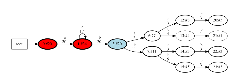
Figure 4. The red-blue framework corresponding to the union/find sets from Figure 3. The red states are the identified parts of the automaton. The blue states are the current candidates for merging. The uncolored states are pieces of the prefix tree that can, at this stage, only be merged during determinization. Currently only state 3 is a merge candidate. The merges of state 3 with 0 and state 3 with 1 will be tested by FlexFringe. If consistent, the highest scoring merge will be performed. If both are inconsistent, state 3 will be colored red and state 6 and 7 will be colored blue.

Algorithm 2 State-merging in the red-blue framework

0:  a data set $D$

0:  $\mathcal{A}$ is a small PDFA that is consistent with $D$

  construct the prefix tree $\mathcal{A}$ from $D$

  color the start state of $\mathcal{A}$ red and all of its children blue

  while  $\mathcal{A}$ contains blue states  do

     for  every blue state $q^{\prime}$  do

        for  every red state $q$  do

           call $\textsc{consistent}={\sf merge}(\mathcal{A},q,q^{\prime})$, compute the merge score

           call ${\sf undo\_merge}(\mathcal{A},q,q^{\prime})$

        end for

     end for

     if  one of the merges is consistent  then

        perform the consistent ${\sf merge}(\mathcal{A},q,q^{\prime})$ with highest score

     else

        color the first blue state in a given order red

     end if

     color all children of red states in $\mathit{A}$ blue

  end while

  return  $\mathit{A}$

3.2. Improvements to red-blue state-merging

In the grammatical inference community, there has been much research into improving merging in the red-blue framework. Initially, state merging algorithms [OG92, CO94] used an order that colors shallow states first, i.e., those closer to the start state or root of the prefix tree. In [Lan99], it was instead suggested to follow an order where the most constrained state is colored first. In FlexFringe, we typically use a largest first order, which colors the most frequent states first. The simple reason for this is that states with large frequency contain more information and thus merges are based on more evidence. In practice this leads to better automata. You can set these different orders in FlexFringe using the shallowfirst and largestblue input parameters. You can also modify whether FlexFringe should change the color of any blue state without consistent merges to red (parameter extend). These extend operations may violate the merge order. It is even allowed to consider merges between pairs of blue states (parameter blueblue). How to set these order influencing parameters is an open problem and highly dependent on the data and use-case. In FlexFringe, we provide parameter presets that exactly mimic the original state merging algorithms from the literature.

In addition to greedily following a predefined order, different search strategies have been studied such as dependency directed backtracking [OS98], using mutually (in)compatible merges [ACS04], iterative deepening [Lan99], beam-search [BO05], and sat-solving [HV10]. Most of these have been studied when learning DFA classifiers, i.e., when both positive and negative data is available. When learning PDFAs, search strategies have been less studied. Most PDFA learning algorithm rely on greedy procedures, some with PAC-bounds that guarantee performance when sufficient data is available [CG08, CT04, BCG13]. There exist some works that minimize Akaike’s Information Criterion (AIC) [Ver10], or a Minimum Description Length measure [AV07]. In FlexFringe, a best-first beam-search strategy is implemented that minimizes the AIC. We are currently working on implementing more search strategies including the use of SAT solvers when learning PDFAs.

3.3. FlexFringe’s parameters

FlexFringe is build to offer flexibility in the type of merging strategy a user wants to apply. Every dataset is different and can use a different way to perform the basic state-merging algorithm. The core red-blue state-merging functionality cannot be changed. Thus, FlexFringe can only learn deterministic automata. Many parameters can be used to change the way this framework is applied. We list the most important ones in Table 1. These are discussed in more detail in different sections in this paper.

largestblue	when set to true only the most frequent blue state is considered
shallowfirst	when set to true only the most shallow blue state is considered
extend	extend (color red) blue states that cannot be merged with any red
blueblue	whether to allow merges between pairs of blue states
redfixed	merges that add new transitions to red states are inconsistent
markovian	states with different that incomming transition symbol are inconsistent
ktail	only perform merge consistency checks up to this depth
sinkson	whether to sink states (unmergeable blue states)
sink_count	states with smaller frequency counts are sinks
state_count	the minimum count for a state to be used in consistency tests
symbol_count	the minimum count for a symbol to be used in consistency tests
correction	Laplace smoothing addition to every symbol count after pooling
finalprob	when set to true final probabilites are computed and used in tests
confidence_bound	the input parameter used by (statistical) consistency checks
mode	whether to use FlexFringe in greedy batch, search, or predict mode
apta_file	a path to a learned automaton (apta), e.g., for making predictions

Table 1. A list of parameters that influence the basic operation of FlexFringe and their meaning. The are discussed in more detail in Sections 3.2, 5.1-5.4., and 6

4. Implemented evaluation functions

Given a potential merge state pair $(q,q^{\prime})$, an evaluation function has to implement a consistency check and a score. As mentioned above, the consistency check is used to determine whether a merge is feasible. The score evaluation is used to determine which merge to perform from a set of consistent ones. In FlexFringe, both of these functions are user defined. For learning PDFAs, FlexFringe provides several well-known consistency checks, which we describe below along with their score computation. Note that these evaluation functions are applied to all pairs of states merged during determinization (the recursion in Algorithm 1). In other words, each merge calls these functions multiple (sometimes hundreds) of times. It is therefore important that they are fast to compute. For instance, FlexFringe always computes counts incrementally and only for the states that get merged during the determinization procedure and the merge itself.

4.1. Counts

All consistency checks use state and symbol counts to determine consistency. These are maintained by FlexFringe in each state using standard maps. Every time a merge is done or undone, the counts in these maps are updated. Since this has to be done for each pair of states merged during determinization, this is typically the most run-time intensive part of the merge procedure. FlexFringe therefore only performs such updates when the counts are used. For instance, they are not maintained when learning deterministic automata using the evidence-driven state-merging algorithm. To implement the well-known checks for learning PDFAs, FlexFringe maintains counts that are used to compute the following:

• $C(q)$: the frequency count of state $q$.

• $C(q,a)$: the frequency count of symbol $a$ in state $q$.

• $S(q,a)$: the probability of symbol $a$ in state $q$.

• $F(q)$: the final probability of state $q$.

• $|\mathcal{A}|$: the number of transitions in PDFA $\mathcal{A}$.

4.2. Alergia

Alergia [CO94] is one of the first and still a very successful algorithm for learning PDFAs. It relies on a test derived from the Hoeffding bound to determine merge consistency checks. For each potential merge pair $(q,q^{\prime})$, it tests for all $a\in\Sigma$ whether

$$\left|S(q,a)-S(q^{\prime},a)\right|<\sqrt{\frac{1}{2}\ln\frac{2}{\alpha}}\left(\frac{1}{\sqrt{C(q)}}+\frac{1}{\sqrt{C(q^{\prime})}}\right)$$

where $\alpha$ is a user-defined parameter, which is set in FlexFringe using the confidence_bound parameter. When using final probabilities, the final probability function $F$ is used in the same way as the symbol probability function $S$ (this holds for all evaluation functions). The Alergia check guarantees that for every pair of merged states, the outgoing symbol distributions are not significantly different. In the original Alergia paper, the state merging algorithm does not implement a score. Instead, it defines a shallow first search order and iteratively performs the first consistent merge in this order. In FlexFringe, Alergia is implemented with the default score of summing up the differences between left-hand and right-hand sides of the above equation over all pairs of tested states, i.e., the used score is:

$$\sum_{q,q^{\prime}}\left(\sqrt{\frac{1}{2}\ln\frac{2}{\alpha}}\left(\frac{1}{\sqrt{C(q)}}+\frac{1}{\sqrt{C(q^{\prime})}}\right)-\left|S(q,a)-S(q^{\prime},a)\right|\right)$$

where $q$ and $q^{\prime}$ are all pairs of states tested during determinization. The larger these differences, the more similar are the tested distributions. In addition, this score prefers merges that perform many merges during determinization. The underlying intuition is that a consistency check is performed for every performed merge. Hence, we are more certain of the consistency of merges that merge more states.

4.3. Likelihood-ratio

A likelihood-ratio test is introduced in  [VWW10] to overcome a possible weakness of Alergia. In Alergia, each pair of merged states is tested independently. When determinization merges hundreds of states, we should not be surprised that a small number of these tests fail. This prevents states from merging, resulting in a larger PDFA. The likelihood-ratio test aims to overcome this by computing a single test for the entire merge procedure, including determinization. It compares the PDFA before the merge $\mathcal{A}=\{\Sigma,Q,q_{0},\delta,S,F\}$ to the PDFA after the merge $\mathcal{A}^{\prime}=\{\Sigma,Q^{\prime},q_{0}^{\prime},\delta^{\prime},S^{\prime},F^{\prime}\}$, computing their log-likelihood and the number of parameters. The log-likelihood of a PDFA is simply the log of all probabilities it assigns to the training data $\sum_{s\in D}\log(\mathcal{A}(s))$. The number of parameters is the number of transitions $|\mathcal{A}|$. Because the two models are nested ($\mathcal{A}^{\prime}$ is a restriction/grouping of $\mathcal{A}$), we can compute a likelihood-ratio test to determine whether parameter reduction outweighs the decrease in likelihood. When it does, a merge is considered consistent. The function it computes is:

$$\chi^{2}\left(2\sum_{q\in Q,a\in\Sigma}C(q,a)\log(S(q,a))-2\sum_{q^{\prime}\in Q^{\prime},a\in\Sigma}C(q^{\prime},a)\log(S^{\prime}(q^{\prime},a)),|\mathcal{A}|-|\mathcal{A}^{\prime}|\right)>\alpha$$

where $\alpha$ is a user-defined parameter (confidence_bound), $\chi^{2}(v,n)$ is the value of $v$ in the chi-squared distribution with $n$ degrees of freedom. In the case that $C(q,a)$ equals $0$, $C(q,a)\log(S(q,a))$ is set to $0$. In FlexFringe, this function is computed incrementally by tracing which parameters get removed during a merge and its effect on the loglikelihood. As score, likelihood-ratio uses 1 minus the p-value obtained from the $\chi^{2}$ function. A larger score indicates that the decrease in likelihood is less significant, i.e., that the distributions modeled by $\mathcal{A}$ and $\mathcal{A}^{\prime}$ are more similar.

4.4. MDI

The MDI algorithm [Tho00] is an earlier approach to overcome possible weaknesses of Alergia, mainly that there is no way to bound the distance of the learned PDFA from the data sample. Like likelihood-ratio, MDI computes the likelihood and the number of parameters. Instead of comparing these directly using a test, MDI uses them to compute the Kullback-Leibler divergence from the models before merging $\mathcal{A}$ and after merging $\mathcal{A}^{\prime}$ to the distribution in the original data sample $D$. The distribution of $D$ is determined using the prefix tree $\mathcal{A}_{p}=\{\Sigma,Q_{p},q_{p,0},\delta_{p},S_{p},F_{p}\}$. When a merge makes this distance too large, it is considered inconsistent:

$$\frac{\left(\sum_{q\in Q_{p},a\in\Sigma}C_{p}(q,a)S_{p}(q,a)\cdot\left(\log(S(\hat{q},a))-\log(S^{\prime}(\hat{q}^{\prime},a))\right)\right)}{|\mathcal{A}|-|\mathcal{A}^{\prime}|}<\alpha$$

where $C_{p}(q,a)$ and $S_{p}(q,a)$ is the count information from the prefix tree $\mathcal{A}_{p}$, $\hat{q}$ and $\hat{q}^{\prime}$ are the states that are merged with $q$ in $\mathcal{A}$ and $\mathcal{A}^{\prime}$ respectively. As before, and $\alpha$ is a user-defined parameter (confidence_bound). The rest is identical to the other evaluation functions, and hence is inherited from the likelihood-ratio implementation. For efficiency reasons, our implementation is slightly different from the original formulation in [Tho00]. We use the counts from $D$ to compute the Kullback-Leibler divergence (similar to likelihood-ratio) instead of computing it directly between the different models. Unfortunately, it is currently not possible to perform a run of the original MDI algorithm which used an exact algorithm (and a lot of run-time) to compute the divergence. This is however the only difference between MDI and its implementation in FlexFringe.

4.5. AIC

The AIC or Akaike’s Information Criterion is a commonly used measure for evaluating probabilistic models  [Aka74]. It is a simple yet effective model selection method for making the trade-off between the number of parameters and likelihood. It is very similar to the likelihood-ratio function but does not rely on the $\chi^{2}$ function. It simply aims to minimize the number of parameters minus the loglikelihood. In [Ver10] this was used to learn probabilistic real-time automata, similar to the use of the minimum description length principle for learning DFAs [AJ06]. In FlexFringe, we simply consider all merges that decrease the AIC as consistent:

$$2\left(|\mathcal{A}|-|\mathcal{A}^{\prime}|\right)-2\left(\sum_{q\in Q,a\in\Sigma}C(q,a)\log(S(q,a))-\sum_{q^{\prime}\in Q^{\prime},a\in\Sigma}C(q^{\prime},a)\log(S^{\prime}(q^{\prime},a))\right)>0$$

Intuitively, this measures whether the reduction in parameters when going from $\mathcal{A}$ to $\mathcal{A}^{\prime}$ is greater than the decrease in loglikelihood. states as evaluation functions, FlexFringe computes this incrementally.

5. Improvements in Speed and Performance

In addition to its efficient implementation and flexibility, FlexFringe introduces several techniques that improve both run-time and performance in state merging. The above evaluation functions work for states that are “sufficiently frequent”. When merging infrequent states, however, they can give bad performance. For instance, Alergia will nearly always merge infrequent states since they will never provide sufficient evidence to determine an inconsistency. As a result, these merges are somewhat arbitrary and can hurt both performance and the insight you can get from the learned models. FlexFringe therefore implements several techniques that deal with low frequency states and transitions.

5.1. Sinks

Sinks are states with user-defined conditions that are ignored by the merging algorithm. The idea of using sinks originated from DFASAT in the Stamina challenge [WLD⁺13, HV13]. In the competition, data was labeled and a garbage state was needed for states that are only reached by negative sequences. Merging such states with the rest of the automaton, thereby combining negative and positive sequences, can only lower performance. In PDFAs, the default condition defines sinks as states that are reached less than sink_count (a user-defined parameter) times by sequences from the input data $D$. In FlexFringe’s merging routines, sinks are never considered as merge candidates, i.e., blue states that are sinks are ignored. They are however merged normally during determinization. (Since the counts from merged states are combined), sinks can become more frequent and thus become a merge candidate in a subsequent iteration. The merging routines continue until all remaining merge candidates are sinks. By default, these sinks and their future states are not output to the automaton model. The transitions to sink states, the sink states themselves, and all subsequent states are simply not printed. There are options to add these to the model, or to continue merging them in different ways (e.g., with red states or only with other sinks).

5.2. Pooling

In addition, the statistical Frequency pooling is a common technique to improve the reliability of statistical tests when faced with infrequent symbols/events/bins. The idea is to combine the frequency of infrequent symbols and thus gain confidence in the outcome of statistical tests. When learning PDFAs, frequency pooling is very important as the majority of states that are merged during determinization are infrequent. Every blue state that is considered for merging is the root of a prefix tree with frequent states near the root and infrequent states in all of its branches. Pooling can be quite straightforward, for example, one can simply combine the counts of symbols that occur less that a user-defined threshold in either or both states of the merge pair. We noticed, however, that straightforward pooling strategies can miss obvious differences:

	a	b	c	d	e	f	g	h	pool
$q$	5	5	5	2	2	1	0	0	20
$q^{\prime}$	0	0	1	2	2	5	5	5	20

Although states $q$ and $q^{\prime}$ are different, the pooled counts (combining columns that have cells with count less than 5) show that they are identical. This creates problems for state merging as the algorithm will consider such merges consistent while clearly they are not. Merging these small counts can have a large effect on the final model since they are added to the representative state $q$ (see Algorithm 1). This thus influences all subsequent statistical tests performed on $q$. Moreover, this effect can be large since there are many states with small counts in the prefix tree. In FlexFringe, we therefore opted to perform a different pooling strategy, with the aim of not hiding these differences. We build two pools:

	a	b	c	d	e	f	g	h	pool1	pool2
$q$	5	5	5	2	2	1	0	0	19	5
$q^{\prime}$	0	0	1	2	2	5	5	5	5	19

The first pool sums the frequency counts for all symbols that occur strictly less the threshold 5 in $q$ (d, .., h), the second those in $q^{\prime}$ (a, .., e). The counts that occur infrequently in both states are added to both pools. The parameter in FlexFringe used for this threshold setting is symbol_count. When learning a PDFA model for a software system, it can make sense to set this parameter to 1. This causes the merging process to be more influenced by the absence/presence of symbols, which is often important for software processes.

The statistical tests in FlexFringe ignore states that have an occurrence frequency lower than state_count. This means that during determinization, whenever one of the two states that are being merged is infrequent, it still performs the merge but does not compute a statistical test. This is especially important for the likelihood ratio tests, which can be influenced by a large amount of infrequent states being merged. Using the state_count parameter, these counts are not added to the likelihood value, and the size reduction (number of parameters) is also not taken into account. FlexFringe also uses a Laplace smoothing by adding correction counts (default 1) to every frequency count after pooling.

5.3. Counting parameters

Many evaluation functions require the counting of statistical parameters before and after a merge. A statistical parameter is a stochastic variable that is estimated from data, such as the sample mean or variance. For a PDFA $\mathcal{A}=\{\Sigma,Q,q_{0},\delta,S,F\}$, these are the parameters that together determine $S$ and $F$ since these are used to assign probabilities to sequences. Because the models before and after a merge are nested, we can compute powerful statistical tests such as the likelihood ratio. A problem is how to compute the reduction in number of parameters. Because a merge can combine many states during determinization, counting one parameter more or less for each state greatly influences the resulting automaton model.

Each state contains statistical parameters for estimating the $S$ and $F$. Essentially one for every possible symbol plus one for the final probability. Since automata are frequently sparse in practice, it makes little sense to include parameters for symbols that do not occur, i.e., symbols $a$ for which $S(q,a)=0$. Counting parameters for these would give a huge preference to merging as every pair of merged states reduces this amount by the size of the alphabet $|\Sigma|$. Instead, we opted to count an additional parameter only for symbols that have non-zero counts in both states before merging. In other words, we count every transition as a parameter. This implies that we measure the size of a PDFA by counting the number of transitions instead of the more common measure of counting the number of states.

5.4. Merge constraints

In addition to ways to deal with low frequency counts and symbol sparsity, FlexFringe contains several parameters that influence which merges are considered. For PDFAs, one of the the most important parameters is largestblue. When set to true, FlexFringe only considers merges with the most frequently occurring blue state. This greatly reduces run-time because instead of trying all possible red-blue merge pairs (quadratic), it only considers merges between all red states with a single blue state (linear). It typically also improves performance, as merging the most frequent states first simply makes sense when testing for consistency using statistical tests. The finalprob parameter is also important. When set to true, it causes FlexFringe to model final probabilities $F$ (learning distributions over $\Sigma^{*}$ instead of $\Sigma^{n}$). When set to false, it sets $F(a)=0$ for every $a\in\Sigma$. This setting should only be used when the ending of sequences contains information, e.g., not when learning from sliding windows that start and end arbitrarily.

When learning PDFAs, there are several other parameters that can be useful to try. Firstly, redfixed makes sure that merges cannot add new transitions to red states, when they do they are considered inconsistent. The key idea is that the red states are already learned/identified, and we should therefore not modify their structure. This does not restrict modifications to their symbol and final probabilities. Secondly, blueblue allows merges between pairs of blue states in addition to red-blue merges. Although state merging in the red-blue framework is complete in the sense that it can return any possible automaton, sometimes it can force a barely consistent merge. Allowing blue-blue merge pairs can avoid such merges. Thirdly, markovian creates a Markov-like constraint. It disallows merges between states with different incoming transition labels when set to $1$. When set to $2$ (or $3$, …), it also requires their parents (and their parents, …) to have the same incoming label. When running likelihood-ratio with a very low statistical test threshold (or negative), and markovian set to 1, it creates a Markov chain. With a larger setting, it creates an n-Gram model. Combined with one of the statistical consistency checks described above, it creates a deterministic version of a labeled Markov chain [ACD91]. Finally, FlexFringe also implements the well-known kTails algorithm for learning automata often used in software engineering [BF72], i.e., only taking futures sequences up to length $k$ into account, which can be accessed using the ktail parameter.

5.5. Searching

Much of the efficiency in FlexFringe is achieved by making use of a union/find data structure, which allows to quickly perform and undo merges. The majority of the time is typically spend on reading, writing, and updating the data structures maintained by the evaluation function which implements the consistency and score functions. A search algorithm calls these functions frequently, but only when evaluation new paths to search. Search routines can therefore quickly switch to different merge paths (undoing and redoing merges) by only performing union/find updates. In this way, FlexFringe can try to optimize a global objective. For PDFAs, it minimizes the AIC of the resulting model. We have implemented a simple best-first search strategy similar to ed-beam [BO05] for this purpose.

6. An example run

We give an example runs of FlexFringe that demonstrate its ease of use and how to use the output given by FlexFringe to decide on parameter values. We run FlexFringe from the command line using Alergia on the data from Figure 1.

./flexfringe --ini ini/alergia.ini test_paper.dat

The first argument gives the initialization file (alergia.ini), which contains parameters for running the Alergia algorithm:

[default]
heuristic-name = alergia
data-name = alergia_data
confidence_bound = 0.95
largestblue = 1
finalprob = 1

This specifies which class files to use for evaluation and data processing (alergia). Specifying this at run-time makes it easy to switch to a different underlying algorithm. Moreover, people interested in developing their own evaluation function heuristic can do so by adding only a single file to the code-base. We set Alergia to use final probabilities and a largest blue search order. The confidence_bound ($\alpha$ parameter used in the consistency check) is set to 0.95, which is much higher than the default of 0.01. This makes it possible to learn models when presented with only 20 traces. With its default setting, FlexFringe cannot distinguish states from each other and learns a single state automaton when given such few traces.

The second argument to FlexFringe provides the training data as input (the data from Figure 1). Executing the above call to FlexFringe provides the following output:

Using heuristic alergia
Creating apta using evaluation class alergia
batch mode selected
starting greedy merging
 x20  m5.0184  x20  m2.45255  m2.08965 no more possible merges
deleted merger

Flexfringe first prints checks for the selected evaluation function and search strategy. After that it outputs information on every performed merge and core extension (coloring a node red). The first output x20 means it extends the core with a state with frequency 20. The second output m5.0184 means it performed a merge with score 5.0184 (summed differences between left-hand side and right-hand side of the performed Alergia tests, see Section 4). This output can be made more verbose, it then also prints the state numbers. It ends when no more merges can be performed and prints whether it successfully freed all allocated memory.

When using FlexFringe, the output can be useful in guiding parameter settings. It can for instance happen that merges are performed with very low scores (printing m0). Such merges can be caused by merging low frequency states or an incorrect merge order. You can try to avoid them by changing parameters such as the use of sinks.

As output, FlexFringe provides two files:

test_paper.dat.ff.final.dot
test_paper.dat.ff.final.json

The dot formatted file is for visualization purposes only. Graphviz dot produces Figure 2 when given this as input. The json file can be used for further processing by FlexFringe to make predictions. This is done by calling FlexFringe in predict mode:

./flexfringe --ini ini/alergia.ini test_paper_test.dat --mode=predict
--aptafile=test_paper.dat.ff.final.json --correction=0

Which runs the predict function with the PDFA specified by the json input on the data argument. We provide an additional argument that disables Laplace smoothing, overriding the ini file and simplifying the probability calculations. We run it on a small test containing only the trace ”a b a b a”. This produces a csv-formatted file as output containing:

state sequence; score sequence
[1,2,1,2,1,1]; [0,-0.510826,-1.60944,-0.510826,-1.60944,-inf]

As can be seen in Figure 1, the state sequence corresponds to the sequence of states visited by the trace ”a b a b a”. At the end, it contains state number 1 twice to denote the state the trace ends in. The scores are the log-probabilities with base $e$ for each state-symbol combination. The trace always starts with an ”a” (log-probability 0). Afterwards it gives the log-probability of producing a ”b” symbol in state 1:

$$\ln(\frac{C(1,b)}{C(q)})=\ln(\frac{30}{50})\approx-0.51$$

The score sequence ends with ”-inf” since it tries to compute the log-probability of ending in state 1. Without smoothing, this probability is 0, giving an infinite negative score. Thus, the trace ”a b a b a” can be labeled as an anomaly.

FlexFringe comes with a Python wrapper for making the above calls for convenience. This makes it easier to integrate FlexFringe into existing Python data processing pipelines. Moreover, in addition to being open-source, FlexFringe contains pre-compiled binaries for Windows, Mac, and Linux. Tutorials on how to setup and use FlexFringe are also available online in the FlexFringe repository .

7. Results on PAutomaC

To demonstrate the value of the improvements made to general state merging algorithms in FlexFringe, we run each of the evaluation functions on the PAutomaC problem set and compare FlexFringe’s performance to the competition winners. PAutomaC was a competition on learning probability distributions over sequences held in 2012 [VEDLH14]. In the competition data there are 48 data sets with varying properties such as the type of automaton/model that was used to generate the sequences, the size of the alphabet, and the sparsity/density of transitions. Since deterministic automata can approximate non-deterministic automata [DDE05], algorithms for deterministic algorithms (such as FlexFringe) can be used for non-deterministic target models. One of the key findings from the PAutomaC competition, however, was that algorithms for learning non-deterministic models perform better when the target is non-deterministic. For evaluation, a test set is provided of unique traces. The task was to assign probabilities to these traces. For evaluation, the assigned probabilities were compared to the ground truth (probabilities assigned by the model that generated the data) using a perplexity metric:

$$Score(C,T,D)=2^{-\sum_{x\in D}P_{T}(x)*log(P_{C}(x))}$$

where $C$ is a submitted candidate model, $T$ is the target model, $D$ is the data set of testing sequences, $P_{T}(x)$ is the normalized probability of $x$ in the target and $P_{C}(x)$ is the normalized candidate probability for $x$ submitted by the participant. The perplexity score measures how well the differences in the assigned probabilities matched with the target probabilities assigned by the ground truth model.

To avoid 0 probabilities in $P_{T}(X)$, we use Laplace smoothing with a correction of 1. We compare the performance of FlexFringe using different heuristics and parameters to the PAutomaC winner (a Gibbs sampler by Shibata-Yoshinaka), and the best performing method on deterministic models (a state merging method by team Llorens). The scores for Shibata-Yoshinaka and team Llorens we obtained from the PAutomaC competition paper [VEDLH14]. We first demonstrate the effectiveness of sinks, low frequency counts, and other improvements using Alergia.

Nr	Model	Solution	Shibata	Llorens	Alergia94	Alergia+	Likelihood	MDI	AIC
6	PDFA	66.99	67.01	67.00	74.05	67.01	67.00	67.54	67.00
7	PDFA	51.22	51.25	51.26	82.92	51.24	51.24	51.46	51.24
9	PDFA	20.84	20.86	20.85	22.22	20.85	20.85	20.99	20.85
11	PDFA	31.81	31.85	32.55	76.53	31.84	31.85	33.56	31.84
13	PDFA	62.81	62.82	62.82	65.01	64.76	64.86	62.87	62.82
16	PDFA	30.71	30.72	30.72	33.49	30.72	30.72	30.78	30.72
18	PDFA	57.33	57.33	57.33	67.04	57.33	57.33	57.39	57.33
24	PDFA	38.73	38.73	38.73	39.63	38.73	38.73	38.91	38.73
26	PDFA	80.74	80.83	80.84	112.01	80.89	80.91	83.52	80.98
27	PDFA	42.43	42.46	42.46	80.52	42.46	42.46	43.49	42.47
32	PDFA	32.61	32.62	32.62	33.28	32.62	32.62	32.65	32.62
35	PDFA	33.78	33.80	34.30	72.29	33.80	33.80	36.81	33.81
40	PDFA	8.20	8.21	8.21	9.66	8.26	8.67	8.52	8.23
42	PDFA	16.00	16.01	16.01	16.14	16.01	16.01	16.05	16.01
47	PDFA	4.119	4.12	4.12	4.65	4.12	4.12	4.13	4.12
48	PDFA	8.04	8.04	8.19	11.73	8.04	8.04	8.24	8.04
1	HMM	29.90	29.99	30.40	34.01	31.98	31.58	31.20	31.19
2	HMM	168.33	168.43	168.42	171.21	168.43	168.43	168.96	168.43
5	HMM	33.24	33.24	33.24	34.65	33.24	33.24	33.31	33.24
14	HMM	116.79	116.84	116.84	117.88	116.84	116.85	117.13	116.85
19	HMM	17.88	17.88	17.92	18.60	17.97	17.98	17.92	17.92
20	HMM	90.97	91.00	93.50	149.44	92.36	91.86	98.61	91.68
21	HMM	30.52	30.57	32.22	83.40	35.25	35.47	37.31	33.52
23	HMM	18.41	18.41	18.45	18.84	18.49	18.44	18.47	18.45
25	HMM	65.74	65.78	67.27	101.97	67.26	68.24	66.83	66.96
28	HMM	52.74	52.84	53.20	60.83	53.77	53.05	53.55	53.02
33	HMM	31.87	31.87	32.03	32.21	31.96	31.95	32.64	31.97
36	HMM	37.99	38.02	38.41	40.88	38.87	38.25	38.29	38.32
38	HMM	21.45	21.46	21.60	24.02	21.84	21.49	21.49	21.49
41	HMM	13.91	13.92	13.94	14.06	14.02	13.98	13.98	14.02
44	HMM	11.71	11.76	12.04	12.62	12.70	12.01	12.04	12.04
45	HMM	24.04	24.05	24.05	24.05	24.04	24.04	24.24	24.04
3	PNFA	49.96	50.04	50.68	52.27	51.35	50.65	51.21	50.65
4	PNFA	80.82	80.83	80.84	82.30	80.95	80.93	80.89	81.02
8	PNFA	81.38	81.40	81.71	91.23	83.01	84.83	82.05	82.73
10	PNFA	33.30	33.33	34.04	49.51	33.65	35.62	35.04	33.47
12	PNFA	21.66	21.66	21.77	23.78	21.68	21.68	22.49	21.68
15	PNFA	44.24	44.27	44.70	52.29	45.10	48.69	46.80	44.66
17	PNFA	47.31	47.35	47.92	60.60	48.03	47.95	51.13	48.11
22	PNFA	25.98	25.99	26.08	39.25	26.56	27.26	26.61	26.37
29	PNFA	24.03	24.04	24.11	27.80	24.20	24.64	24.58	24.15
30	PNFA	22.93	22.93	23.21	26.05	23.47	23.25	23.33	23.22
31	PNFA	41.21	41.23	41.62	43.00	42.08	41.51	42.27	41.60
34	PNFA	19.96	19.97	20.54	36.27	25.99	43.01	26.50	22.63
37	PNFA	20.98	21.00	21.02	21.11	21.19	21.07	21.11	21.13
39	PNFA	10.00	10.00	10.00	10.34	10.00	10.00	10.05	10.00
43	PNFA	32.64	32.72	32.78	33.30	33.14	32.97	32.85	33.05
46	PNFA	11.98	11.99	12.10	15.55	12.50	13.02	12.89	12.43

Table 2. PAutomaC problems, sorted according to model types (HMM = hidden Markov model, PNFA = probabilistic non-deterministic automaton), and perplexity scores of top two teams in PAutomaC and FlexFringe with different evaluation functions. Best scores are bold. The solution column gives the best possible perplexity score.

7.1. Alergia improvements

The results are given in Table 2. We first run Alergia as written in the 1994 seminal paper [CO94]. Out-of-the-box (column Alergia94), this performs not very well and a very likely reason for this is the effect of low frequency counts on the consistency test and the resulting bad merges. When we change the shallow-first merge order into largest-blue, the performance improves. Adding sinks also improves the performance, as well as the run-time. We use a sink_count of 25, which causes FlexFringe to complete the full set of PAutomaC training files in 20 minutes on a single thread at 2.6 GHz. We did not tune the threshold parameter and kept it at its default value of $0.01$.

The results become competitive when running Alergia with our new pooling strategy (column Alergia+) in addition to using sinks. We use a state_count of 15, and a symbol_count of 10. Note that state_count has to be lower than sink_count. If not, merging states with frequency below state_count is considered valid. But since sinks are not used at all during consistency or score computations, they can be merged with any other state. It is best to avoid performing merges without evidence.

Alergia+ achieves much better scores than Alergia. FlexFringe performs particularly well when compared with the best performing state merging approach at the time of the competition (Llorens). The competition winner’s Gibbs sampling approach is hard to beat on all problems, in particular those where the ground truth model is non-deterministic. For the PDFA ground truth models, the performance is close to optimal. We emphasize, however, that we did not tune the confidence_bound parameter used by the statistical tests or run FlexFringe’s search procedure to obtain these results.

7.2. Other evaluation functions

We also evaluate the likelihood-ratio, MDI, and AIC evaluation functions (consistency and score computations) to demonstrate that the choice of function can have a large effect on the obtained performance. In fact, one of the main reasons we developed FlexFringe is to be able to design a new evaluation function quickly. We believe that different problems not only require different parameter settings, but often require different evaluation functions. In a way, this is similar to the use of different loss functions when training neural networks.

We run these different evaluation functions with the same settings for sink_count, symbol_count, and state_count, and their default confidence_bound parameter. The results from likelihood-ratio seem slightly worse than the results we obtain from our modified Alergia. Although it achieves competitive scores on many problems, on several problems, the obtained perplexity scores are much larger.

Out-of-the-box, MDI also seems to perform worse than Alergia+, though it shows smaller deviations than out-of-the-box likelihood-ratio, in particular on problem 21. Interestingly, and unexpectedly, AIC performs best out-of-the-box. Ignoring empty lines, the code for AIC is about 20 lines long. This result shows the key strength of FlexFringe: the ability to quickly implement new evaluation functions. We did not expect AIC to work so well based on earlier results [Ver10]. These results indicate that our pooling and parameter counting strategies have a positive effect on model selection criteria.

8. Results on HDFS

The HDFS data set [XHF⁺09] is a well-known data set for anomaly detection and has for instance been used to evaluate the DeepLog anomaly detection framework based on neural networks [DLZS17]. The first few lines of the training file given to FlexFringe is shown in Figure 5. As can be seen, this data contains patterns that are quite typical in software systems such as parallelism, repetitions, and sub-processes. Although FlexFringe does not specifically look for such patterns (yet), the deterministic nature of the models learned by FlexFringe does offer advantages over the use of neural networks. Firstly, since software is usually deterministic, automaton models provide insight into the software process that generated the data when visualized. Secondly, again due to software’s deterministic nature, learned automata provide excellent performance on problems such as sequence prediction and anomaly detection. Thirdly, learning automata is much faster. FlexFringe requires less than a second of training time to returns good performing and insightful models from the HDFS training data.

4855 50
1 19 5 5 5 22 11 9 11 9 11 9 26 26 26 23 23 23 21 21 21
1 13 22 5 5 5 11 9 11 9 11 9 26 26 26
1 21 22 5 5 5 26 26 26 11 9 11 9 11 9 2 3 23 23 23 21 21 21
1 13 22 5 5 5 11 9 11 9 11 9 26 26 26
1 31 22 5 5 5 26 26 26 11 9 11 9 11 9 4 3 3 3 4 3 4 3 3 4 3 3 23 23 23 21 21 21
    

Figure 5. The first six lines of the HDFS training data provided to FlexFringe in Abbadingo format [LPP98]. The first line gives the number of sequences and the alphabet size. Then each line presents a sequence by specifying the sequence type, length, and the sequence itself as a list of symbols. All traces have type 1, meaning they are all valid system occurrences. When multiple classes or sequences types are available, you can specify the type here in order to learn a classifier. In this use case, we learn a probabilistic model and do not care about sequence types. From these few sequences, we already see several subprocesses with symbols: 5s-22s at the start, 11s-9s in the middle, and 23s-21s at the end. Optionally 2s-3s-4s appears before the 23s-21s. FlexFringe will capture such structures and more hidden ones.

We obtained the data from the DeepLog GitHub repository. The training data consists of 4855 training traces (all normal), 16838 abnormal testing traces, and 553366 normal testing traces. We thus see only a small fraction of the normal data at training time. Despite this restriction, DeepLog shows quite good performance on detecting anomalies [DLZS17]: 833 false positives (normal labeled as abnormal) and 619 false negatives (abnormal labeled as normal). We now present the results of FlexFringe on this data, first in terms of insight then in terms of performance.

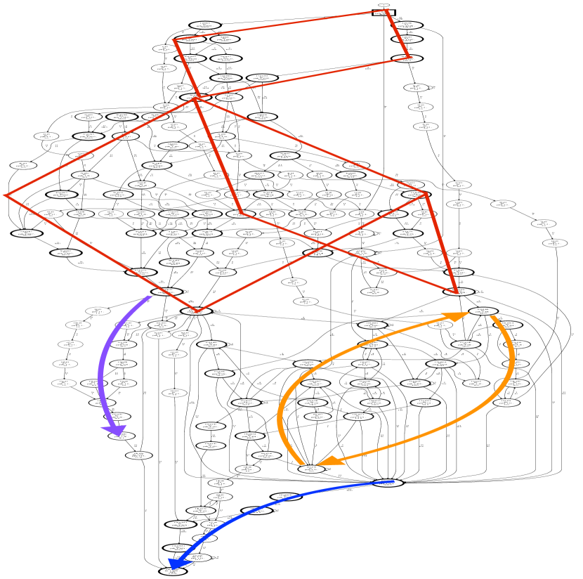
Figure 6. The result of FlexFringe’s AIC heuristic without tuning on the HDFS data set. We see clear parallelism in the top, chains of events at the left bottom, repetitions (loops) in the right bottom, and a short sequence of ending events. The thicknesses of the states are an indication of their frequency.

8.1. Software process insight

For getting initial insight into the data, we run the AIC evaluation function out-of-the-box on the training data. The result is shown in Figure 6. We can clearly distinguish subprocesses and parallelism. The top half process forms a narrow-wide-narrow shape indicative of parallel executions. The initial parallel processing consisting of 22 and 5 values is followed by three 26s and three pairs of 11s and 9s. These can all be executed in parallel, causing a very wide model containing (at least) one state for every possible set of previously executed values. Around half-way through the model, the processing continues starting from just two frequent and one infrequent state. Figure 7 shows the subgraph for the initial parallel processing of 22 and 5 values in more detail. A 22 value can and does occur before, during, or after three occurrences of a 5 value. Interestingly, this processing ends in a different state (17 instead of 14) when a 22 is followed by three 5s. Although the subsequent processing is identical, this is makes sense due to the large difference in frequency of the subsequent 11 value. The parallel processing of 9s, 11s, and 26s is similar but much more complicated.

The field of process mining [VDA12] is focused on methods that explicitly model such behavior using Petri Nets. These only require a only a single transition for a parallel event such as the 9, 11, and 26 values in the HDFS data. Automata can model parallel behavior, but at a great cost in model size since every possible set of previously seen values requires a unique state. Since the bias of automaton learning is to minimize this size, it is nice to see that FlexFringe is able to discover this behavior from only a few thousand traces. In future work, we aim to extend FlexFringe to actively search for such behavior and complete the obtained models. For instance, if we observe $abc$, $cba$, $bac$, and $cab$, we would like to infer that $acb$ is also possible. The current merging routines are unable to do so. Note that although process mining techniques can model parallelism, they have much more problems with modeling sequential context and counting (such as a 5 occurring exactly 3 times).

After the initial two processes (forming the diamond), there are two possible subprocesses: an infrequent long chain of executions 25-18-5-6-26-26-21, which can be repeated, and a frequent process with many repetitions of 2s, 3s, and 4s. These processes can also be skipped and the repetitions can end at different points. This can be seen by the many transitions going to the final process consisting of three optional repetitions of 23s and 21s.

Overall, the learned model provides a lot of insight into the structure of the process that generated the logs. We could reach similar conclusions simply by looking at the log files but we cannot look at 4855 log lines in one view, the learned automaton provides such a view. Moreover, it can show patterns that would be hard to find via manual investigation.

For instance after the parallel executions of the 9s, 11s, and 26s, there are two possible futures depending on whether the final symbol is a 9 or 26. In the latter case, starting the 23s and 21s ending sequence is much more likely. When the parallel execution ends with a 9, only 361 out of 1106 traces start this ending. When ending with a 26, these sequences occur 2519 out of 4375 times. This difference causes the learning algorithm to infer there are two states that signify the end of the 9-11-26 parallel execution: state 98 and state 100. These are the frequent (thick edged) states in the middle left and middle right of the automaton model. Another observation is that this 23-21 ending sequence can be started from many different places in the system, but after the initial parallel executions. This can be seen by the many input transitions to state 102, the frequent state in the right bottom part of the model.

The model also shows some strange bypasses of this behavior, for instance the rightmost infrequent path that skips the frequent states after the 9-11-26 parallel executions (rightmost path, middle of the automaton). This path occurs only twice in the entire training data. Consequently, the statistics used to infer this path are not well estimated. It seems likely that the learning algorithm made an incorrect inference, i.e., these frequent states should not be bypassed. We are currently working on techniques to change the bias of FlexFringe to avoid making such mistakes. Note that the only way to identify such issues is by visualizing and reasoning about the obtained models, something that is prohibitively hard for many other machine learning models such as neural nets. This is an important reason why the recent research line of extracting automaton models from complex neural networks is very relevant [WGY18, AEG19, MAP⁺21].

8.2. Anomaly detection performance

Out-of-the-box, the AIC model seems to capture the underlying process behavior and it can therefore be used for anomaly detection. The most straightforward approach, which does not involve setting a decision threshold, is simply to run the test set through the model and raise an alarm either when a trace ends in a state without any final occurrences, or when it tries to trigger a transition that does not exist. This strategy gives 4132 false positives but only 1 false negative. Using the common F1 score as metric, this gives a score of 0.89, which is worse than the 0.96 obtained by DeepLog on the same data.

We can of course improve this performance by tuning several parameters. Before we do so, it is insightful to understand the cause for the somewhat large number of false positives. FlexFringe learns (merges states) by testing whether the future process is independent from the past process. By merging more, it will generalize more, and hence cause less false positives. But should this be our aim?

One of the key strengths of learning a deterministic automaton model is that one can easily follow a trace’s execution path  [HVLS16]. The simplicity of our anomaly detection setup then allows us to reason on the logic of the detection. This kind of explainable machine learning is unheard of in the neural network literature. Investigating the raised false positives provides us with four frequent types of anomalous traces in the normal test set:

Figure 7. A subplot of the PDFA from Figure 6 showing paths taken by the mentioned anomalous traces and several parallel states (fin and path counts removed for clarity). State 7 occurs 1257 times in the training data (of 4855 traces in total) and the subsequent event is always 5 (never 11 as in the different start trace). The infrequent trace reaches state 69 (thick path), there is no outgoing transition with label 26 from state 69. However, we could infer from the parallel paths that the target state should be state 79, i.e., the state reached by swapping the last 11 and 26 events, since it seems these can be executed in parallel.

1. Not starting with a 22 and three 5s, e.g., 22-5-11-9-5-11-9-5-11-9-26-26-26.

2. Following an infrequent paths, e.g., 22-5-5-5-9-26-11-9-11-26…

3. Containing symbols not in the train set, e.g., 22-5-5-5-…-3-4-23-23-23-21-21-20-21.

4. Repetition of values, e.g., 5-5-…-4-4-4-3-4-4-4-4-4-4-4-4-4-4-4-4-2-2-…

To facilitate the analysis of these behaviors, we plot a subgraph from Figure 6 in Figure 7. The different start traces quickly reach a state without a transition for the next symbol. The listed trace ends after the 22 and 5 symbols, the reached state occurred 1257 times by traces from the training data, and all of these traces had 5 as their next symbol. We would argue that this is an anomaly that should be raised. In fact, there are only 63 traces that start with 22-5-11 in the entire test and 139761 that start with 22-5. Still, these are counted as false positives when computing the F1 score.

The infrequent paths end in, or traverse, states that occur infrequently. The listed prefix ends after the second 11 symbol in a state that occurs only 20 times and always had a 9 or 11 as next symbol in the training data. This seems no anomaly and different parameter settings would likely cause a merge of this state, and thus possibly provide a transition with label 26. The sink parameters in FlexFringe can be used to prevent learning models with infrequent occurrences and thus avoid raising such false positives. We argue however that this is bad practice as learning such an infrequent state is no mistake. Many states are required to model the parallelism present in the data, and several of these will be infrequent. Given this parallelism, we actually know what state to target, the one reached by the prefix 22, 5, 5, 5, 9, 26, 11, 9, 26, 11 (state number 79). We simply swapped the last two symbols. This state occurs much more frequently (634 times) and we could simply add this transition (from state 69 to 79 with label 26) to the model. In future work, we aim to either extend a learned automaton with such 0-occurrence transitions or check for them at test time.

The traces with new symbols are clearly abnormal and should be counted as true negatives rather than false positives. The HDFS data is somewhat strange in that events occur in the test set that never occurred at train time. Also many of the true positive traces contain such symbols.

Traces with different repetitions do show mistakes made by the learning algorithm. The repetition subprocess contains many possible repetitions, but apparently still more are possible. Performing more or different merges will change these and potentially remove these false positives. Learning which repetitions are possible and which are not requires more data or a different learning strategy/parameter settings.

Figure 8. The result of FlexFringe’s Likelihoodratio heuristic with a very low confidence_bound. It performs many more merges compared to Figure 6. As a consequence, it is much harder to interpret. We still see some parallelism at the top, but many self loops are likely overgeneralizations. Moreover, the many (probably incorrect) long transitions hinder interpretability. In terms of F1-score, it performs better than the model from Figure 6, and better than the DeepLog baseline [DLZS17]

8.3. A different learning strategy

One way to raise less false alarms is to perform more merges and thus obtain fewer states that have more outgoing transitions. The AIC evaluation function does not have a significance parameter (confidence_bound). Instead, we learn another model using the likelihood-ratio evaluation function and a very low confidence_bound of 1E-15. Other than that, we keep the default settings. The resulting model is displayed in Figure 8. The model is much less insightful than Figure 6 and likely overgeneralizes due to all the added loops. It seems to model impossible system behavior such as infinite loops of 21s. In terms of performance, however, this model achieves 330 false positives and 624 false negatives, i.e., an F1-score of 0.97 outperforming the score achieved by DeepLog.

This demonstrates automaton learning methods can outperform neural network approaches with little fine-tuning on software log data. We believe the main reason for this to be that software data is highly structured and often deterministic. On the experiments on the PAutomaC data, we also demonstrated that deterministic automata learned using FlexFringe perform excellent when the ground truth model is deterministic. Automata are simply good at capturing the type of patterns that occur in deterministic systems.

A key question and challenge for future work is how to treat infrequent states during learning. Is it better to keep them intact to obtain a more interpretable model or should we merge them and get improved performance at cost of interpretability? In order to prevent this trade-off, we are currently extending FlexFringe with methods that look for software specific patterns such as parallelism and subprocesses. We believe that such extensions will be crucial for obtaining high performing interpretable models.

9. Related works

There exist a lot of different algorithms for learning (P)DFAs. Like FlexFringe, most of these use some form of state consistency based on their future behavior, i.e., a test for a Markov property or Myhill-Nerode congruence. Many algorithms are active, these learn by interacting with a black-box system-under-test (SUT) by providing input and learning from the produced output. Starting from the seminal L* work in [Ang87], and its successful implementation in the LearnLib tool [RSB05], many works have applied and extended this algorithm, e.g., to analyze and reverse engineer protocols [FBJV16, FBJM⁺20] and learn register automata [IHS14a, AFBKV15]. Although closely related to learning from a data set [LZ04], since FlexFringe does not learn actively, we will not elaborate more on these approaches and refer to [Vaa17] for an overview of active learning algorithms and their application. Below, we present related algorithms that learn from a data set as input.

9.1. Algorithms

We described the main state-merging algorithms FlexFringe builds upon in Section 3. In the literature, there exist several other approaches. A closely related research line is consists of different versions of the k-Tails algorithm [BF72], essentially a state-merging method that limits consistency until depth k for computational reasons. Moreover, this allows to infer models from unlabeled data without using probabilities: simply require identical suffixes up to depth k. In the original work, the authors propose to solve this problem using mathematical optimization. Afterwards, many greedy versions of this algorithm have been developed and applied to a variety of software logs [CW98]. Notable extensions of state merging methods are the declarative specifications [BBA⁺13], learning from concurrent/parallel traces [BBEK14], and learning guarded, extended, and timed automata [MPS16, WTD16, PMM17, HW16]. Several ways to speedup state-merging algorithms have also been proposed by through divide and conquer and parallel processing [LHG17, ABDLHE10, SBB21]. There have also been several proposals to use different search strategies such as beam search [BO05], genetic algorithms [LR05, TE11], satisfiability solving [HV13, ZSU17], and ant-colony optimization [CU13].

Another closely related line of work focuses on spectral learning methods. Spectral learning formulates the PDFA (or weighted automaton) learning problem as finding the spectral decomposition of a Hankel matrix [BCLQ14, GEP15]. Every row in this matrix represents a prefix, every column a suffix, each cell contains the string probability of the corresponding row and column prefix and suffix. The rows of this matrix correspond to states of the prefix tree. If one row is the multiple of another, it means that the future suffix distribution of the corresponding states are similar, i.e., that they can be merged. Instead of searching for such similarities and forcing determinization, spectral methods approximate this using principal component analysis, returning a probabilistic non-deterministic finite state automaton (PNFA). These are less interpretable (although typically smaller) than their deterministic counterparts, but can be computed more efficiently.

Due to their close relationship with hidden Markov models (HMMs) [DDE05], several approaches exist that infer HMMs instead of PDFAs from trace data. HMMs are typically learned using a form of expectation-maximization known as the Baum-Welch algorithm [RJ86]. However, special state merging [SO92] or state splitting [TS92] algorithms have also been proposed. A notable recent approach [EM18] learns accurate probabilistic extended automata using HMMs combined with reinforcement learning.

9.2. Tools

There exist several implementations of state-merging algorithms that can be found on the internet. We list the most popular ones and highlight differences with FlexFringe.

9.2.1. MINT

[WTD16] is a tool for learning extended DFAs. These contain guards on values in addition to symbols. In MINT, these guards are inferred using a classifier from standard machine learning tools which aim to predict the next event from features of the current event. When triggering a transition, the guard is used together with the symbol to determine the next state. FlexFringe also contains such functionality, but instead of using a classifier, it uses a decision-tree like construction to determine guards. Moreover, FlexFringe uses the RTI procedure for this construction, which requires consistency for the entire future instead of only the next event. Finally, in MINT the learning of these guards is performed as preprocessing. In FlexFringe, it is computed on the fly for every blue state (merge candidate). MINT contains several algorithms including GK-Tails [LMP08], which uses the Daikon invariant inference system [EPG⁺07] to learn guards.

9.2.2. Synoptic and CSight

[BABE11, BBEK14] are tools based on k-Tails style state-merging of non-probabilistic automata. They are focused on learning models for concurrent and distributed systems, contain methods to infer invariants, and can combined with model checkers to verify these invariants against the learned models. When a model fails to satisfy an invariant, it is updated used counter-example guided abstraction refinement (CEGAR) [CGJ⁺00]. Although CEGAR is a common way to implement active learning algorithms, Synoptic and CSight both learn from data sets. From the same lab comes also InvariMint [BBA⁺13], a framework for declaratively specifying automaton learning algorithms using properties specified by LTL formulas. Similar specifications in other first order logic have also been proposed [BBB⁺15]. Such specifications are very powerful and allow for a lot of flexibility in designing learning algorithms, as a new algorithm requires just a few lines of code/formulas. Some properties, such as statistical tests, are quite hard to specify. This is why FlexFringe allows specifications of new evaluation functions by writing code instead of formulas. Currently, FlexFringe does not contain functionality for CEGAR-like refinement, or methods to mine invariants.

9.2.3. GI-learning

[COP16] is an efficient toolbox for DFA learning algorithms written in C++, including significant speedups due to parallel computation of merge tests. It contains implementations of basic approaches for both active algorithms and algorithms that learn from a data set. It is possible to extend to include more algorithms and different types of automata by extending the classes of these basic approaches. FlexFringe makes this easier by only requiring new implementations of the consistency check and score methods. FlexFringe currently contains no methods for parallel processing, but the use of the union/find datastructures (see Section 3) makes FlexFringe already very efficient.

9.2.4. LibAlf

[BKK⁺10] is a well-known extensive library for automaton learning algorithms, both active and for learning from a data set. It includes many standard but also specialized algorithms for instance for learning visibly one-counter automata, and also non-deterministic automata. Like FlexFringe, it is easily extensible but does not include algorithms for learning guards or probabilistic automata.

9.2.5. AALpy

[MAP⁺21] is a recent light-weight active automata learning library written in pure Python. In addition to many active algorithms and optimizations, it also contains basic algorithms for learning from a data set. A key feature of AALpy is its easy of use and the many different kinds of models that can be learned, including non-deterministic ones. It is extensible by defining new types of automata and algorithms. It has a different design from FlexFringe in that a new algorithm requires new implementations of the all merge routines, instead of only the evaluation functions. AALpy currently has no support for inferring guards.

9.2.6. LearnLib

[IHS15] is a popular toolkit for active learning of automata, in particular Mealy machines. It has methods to connect to a software system under test by mapping discrete symbols from the automata’s alphabet to concrete inputs for the software system, such as network packets. In addition, it contains different model-based testing methods [LY96] that are used to find counterexamples to an hypothesized automaton and optimized active learning algorithms such as TTT [IHS14b]. As such, it is frequently used in real-world use-cases, see, e.g., [FBJM⁺20]. There also exist extensions for LearnLib such as the ability to learn extended automata [CHJ15].

9.2.7. Sp2Learn

[ABDE17] is a library for spectral learning of weighted or probabilistic automata from a data set written in Python. It learns non-deterministic automata, which are typically harder to interpret than deterministic ones, but can model distributions from non-deterministic systems more efficiently. Spectral learning can be very effective, as it solves the learning problem using a polynomial time decomposition algorithm. In contrast, FlexFringe’s state-merging methods also run in polynomial time but likely results in a local minimum. Search procedures that aim to find the global optimum are very expensive to run.

9.2.8. DISC

[SLTIM20] is a recent mixed integer linear programming method for learning non-probabilistic automata from a data set. Using mathematical optimization is a promising recent approach for solving machine learning problems such as decision tree learning [CMRRM21, VZ17, BD17]. FlexFringe contains one such approach, but based on satisfiability solvers instead of integer programming. An advantage of DISC is that it can handle noisy data due to the use of integer programming, which uses continuous relaxations during its solving procedure. Due to the explicit modeling of noise, it can handle some types of non-determinism without requiring additional states. FlexFringe does not explicitly model noise, but does allow for more robust evaluation functions such as impurity metrics used in decision tree learning.

10. Conclusion

FlexFringe provides efficient implementations of key state-merging algorithms including optimizations for getting improved results in practice. We presented how to use FlexFringe in order to learn probabilistic finite state automata (PDFAs). It can learn these using a variety of methods such as EDSM, Alergia, RPNI, MDI, AIC, and with different search strategies. The kinds of automata and/or the used evaluation function can be changed by adding a single file to the code base. All that is needed is to specify when a merge is inconsistent and what score to assign to a possible merge. The main restriction compared to existing tools is that the learned models have to be deterministic. This is an invariant we use to speed-up the state-merging algorithm.

FlexFringe obtains excellent results on prediction and anomaly tasks thanks to our optimizations. Moreover, the learned models provide clear insight into the inner workings of black-box software systems. On trace prediction, our results show FlexFringe performs especially well when the data are generated from a deterministic system. On anomaly detection, the model produced by FlexFringe outperforms an existing method based on neural networks while requiring only seconds of run-time to learn. We believe its excellent performance is due to properties of software data such as little noise and determinism favoring automaton models.

We demonstrate that there exists a clear trade-off between the obtained insight and (predictive) performance of models. Sometimes, it is best to keep data intact, e.g., when there is too few data to determine what learning (merging) step to take. FlexFringe provides techniques such as sinks to prevent the state-merging algorithm from performing incorrect merges, which can be detrimental for insight as these often lead to incorrect conclusions. Also, merges with little evidence often lead to convoluted models. For making predictions, however, such convoluted and likely incorrect models perform better due to their increased generalization. This trade-off deserves further study. We expect there exist better generalization methods for software systems that do lead to both improved insight and improved performance.

References

- [ABDE17] Denis Arrivault, Dominique Benielli, François Denis, and Rémi Eyraud. Sp2learn: A toolbox for the spectral learning of weighted automata. In International conference on grammatical inference, pages 105–119. PMLR, 2017.
- [ABDLHE10] Hasan Ibne Akram, Alban Batard, Colin De La Higuera, and Claudia Eckert. Psma: A parallel algorithm for learning regular languages. In NIPS workshop on learning on cores, clusters and clouds. Citeseer, 2010.
- [ABL02] Glenn Ammons, Rastislav Bodik, and James R Larus. Mining specifications. ACM Sigplan Notices, 37(1):4–16, 2002.
- [ACD91] Rajeev Alur, Costas Courcoubetis, and David Dill. Model-checking for probabilistic real-time systems. In Automata, Languages and Programming: 18th International Colloquium Madrid, Spain, July 8–12, 1991 Proceedings 18, pages 115–126. Springer, 1991.
- [ACS04] John Abela, François Coste, and Sandro Spina. Mutually compatible and incompatible merges for the search of the smallest consistent dfa. In International Colloquium on Grammatical Inference, pages 28–39. Springer, 2004.
- [AEG19] Stéphane Ayache, Rémi Eyraud, and Noé Goudian. Explaining black boxes on sequential data using weighted automata. In International Conference on Grammatical Inference, pages 81–103. PMLR, 2019.
- [AFBKV15] Fides Aarts, Paul Fiterau-Brostean, Harco Kuppens, and Frits Vaandrager. Learning register automata with fresh value generation. In International Colloquium on Theoretical Aspects of Computing, pages 165–183. Springer, 2015.
- [AJ06] Pieter Adriaans and Ceriel Jacobs. Using mdl for grammar induction. In Grammatical Inference: Algorithms and Applications: 8th International Colloquium, ICGI 2006, Tokyo, Japan, September 20-22, 2006. Proceedings 8, pages 293–306. Springer, 2006.
- [Aka74] Hirotugu Akaike. A new look at the statistical model identification. IEEE transactions on automatic control, 19(6):716–723, 1974.
- [Ang87] Dana Angluin. Learning regular sets from queries and counterexamples. Information and computation, 75(2):87–106, 1987.
- [ANV11] Joao Antunes, Nuno Neves, and Paulo Verissimo. Reverse engineering of protocols from network traces. In 2011 18th Working Conference on Reverse Engineering, pages 169–178. IEEE, 2011.
- [AV07] Pieter Adriaans and Paul Vitanyi. The power and perils of mdl. In 2007 IEEE International Symposium on Information Theory, pages 2216–2220. IEEE, 2007.
- [AV10] Fides Aarts and Frits Vaandrager. Learning i/o automata. In International Conference on Concurrency Theory, pages 71–85. Springer, 2010.
- [BABE11] Ivan Beschastnikh, Jenny Abrahamson, Yuriy Brun, and Michael D Ernst. Synoptic: Studying logged behavior with inferred models. In Proceedings of the 19th ACM SIGSOFT symposium and the 13th European conference on Foundations of software engineering, pages 448–451, 2011.
- [BBA+13] Ivan Beschastnikh, Yuriy Brun, Jenny Abrahamson, Michael D Ernst, and Arvind Krishnamurthy. Unifying fsm-inference algorithms through declarative specification. In 2013 35th International Conference on Software Engineering (ICSE), pages 252–261. IEEE, 2013.
- [BBB+15] Maurice Bruynooghe, Hendrik Blockeel, Bart Bogaerts, Broes De Cat, Stef De Pooter, Joachim Jansen, Anthony Labarre, Jan Ramon, Marc Denecker, and Sicco Verwer. Predicate logic as a modeling language: modeling and solving some machine learning and data mining problems with idp3. Theory and Practice of Logic Programming, 15(6):783–817, 2015.
- [BBEK14] Ivan Beschastnikh, Yuriy Brun, Michael D Ernst, and Arvind Krishnamurthy. Inferring models of concurrent systems from logs of their behavior with csight. In Proceedings of the 36th International Conference on Software Engineering, pages 468–479, 2014.
- [BCG13] Borja Balle, Jorge Castro, and Ricard Gavaldà. Learning probabilistic automata: A study in state distinguishability. Theoretical Computer Science, 473:46–60, 2013.
- [BCLQ14] Borja Balle, Xavier Carreras, Franco M. Luque, and Ariadna Quattoni. Spectral learning of weighted automata. Machine learning, 96(1):33–63, 2014.
- [BD17] Dimitris Bertsimas and Jack Dunn. Optimal classification trees. Machine Learning, 106(7):1039–1082, 2017.
- [BF72] Alan W Biermann and Jerome A Feldman. On the synthesis of finite-state machines from samples of their behavior. IEEE transactions on Computers, 100(6):592–597, 1972.
- [BIPT09] Antonia Bertolino, Paola Inverardi, Patrizio Pelliccione, and Massimo Tivoli. Automatic synthesis of behavior protocols for composable web-services. In Proceedings of the 7th joint meeting of the European software engineering conference and the ACM SIGSOFT symposium on The foundations of software engineering, pages 141–150, 2009.
- [BKK+10] Benedikt Bollig, Joost-Pieter Katoen, Carsten Kern, Martin Leucker, Daniel Neider, and David R Piegdon. libalf: The automata learning framework. In International Conference on Computer Aided Verification, pages 360–364. Springer, 2010.
- [BO05] Miguel Bugalho and Arlindo L Oliveira. Inference of regular languages using state merging algorithms with search. Pattern Recognition, 38(9):1457–1467, 2005.
- [CBP+11] Chia Yuan Cho, Domagoj Babić, Pongsin Poosankam, Kevin Zhijie Chen, Edward XueJun Wu, and Dawn Song. MACE:Model-inference-Assisted concolic exploration for protocol and vulnerability discovery. In 20th USENIX Security Symposium (USENIX Security 11), 2011.
- [CG08] Jorge Castro and Ricard Gavalda. Towards feasible pac-learning of probabilistic deterministic finite automata. In International Colloquium on Grammatical Inference, pages 163–174. Springer, 2008.
- [CGJ+00] Edmund Clarke, Orna Grumberg, Somesh Jha, Yuan Lu, and Helmut Veith. Counterexample-guided abstraction refinement. In International Conference on Computer Aided Verification, pages 154–169. Springer, 2000.
- [CHJ15] Sofia Cassel, Falk Howar, and Bengt Jonsson. Ralib: A learnlib extension for inferring efsms. DIFTS. hp://www. faculty. ece. vt. edu/chaowang/di s2015/papers/paper, 5, 2015.
- [CKW07] Weidong Cui, Jayanthkumar Kannan, and Helen J Wang. Discoverer: Automatic protocol reverse engineering from network traces. In USENIX Security Symposium, pages 1–14, 2007.
- [CMRRM21] Emilio Carrizosa, Cristina Molero-Río, and Dolores Romero Morales. Mathematical optimization in classification and regression trees. Top, 29(1):5–33, 2021.
- [CO94] Rafael C Carrasco and Jose Oncina. Learning stochastic regular grammars by means of a state merging method. In International Colloquium on Grammatical Inference, pages 139–152. Springer, 1994.
- [COP16] Pietro Cottone, Marco Ortolani, and Gabriele Pergola. Gl-learning: an optimized framework for grammatical inference. In Proceedings of the 17th International Conference on Computer Systems and Technologies 2016, pages 339–346, 2016. URL: https://github.com/piecot/GI-learning.
- [CT04] Alexander Clark and Franck Thollard. Pac-learnability of probabilistic deterministic finite state automata. Journal of Machine Learning Research, 5(May):473–497, 2004.
- [CU13] Daniil Chivilikhin and Vladimir Ulyantsev. Muacosm: a new mutation-based ant colony optimization algorithm for learning finite-state machines. In Proceedings of the 15th annual conference on Genetic and evolutionary computation, pages 511–518, 2013.
- [CW98] Jonathan E Cook and Alexander L Wolf. Discovering models of software processes from event-based data. ACM Transactions on Software Engineering and Methodology (TOSEM), 7(3):215–249, 1998.
- [CWKK09] Paolo Milani Comparetti, Gilbert Wondracek, Christopher Kruegel, and Engin Kirda. Prospex: Protocol specification extraction. In 2009 30th IEEE Symposium on Security and Privacy, pages 110–125. IEEE, 2009.
- [DDE05] Pierre Dupont, François Denis, and Yann Esposito. Links between probabilistic automata and hidden markov models: probability distributions, learning models and induction algorithms. Pattern recognition, 38(9):1349–1371, 2005.
- [DlH10] Colin De la Higuera. Grammatical inference: learning automata and grammars. Cambridge University Press, 2010.
- [DLZS17] Min Du, Feifei Li, Guineng Zheng, and Vivek Srikumar. Deeplog: Anomaly detection and diagnosis from system logs through deep learning. In Proceedings of the 2017 ACM SIGSAC conference on computer and communications security, pages 1285–1298, 2017.
- [EM18] Seyedeh Sepideh Emam and James Miller. Inferring extended probabilistic finite-state automaton models from software executions. ACM Transactions on Software Engineering and Methodology (TOSEM), 27(1):1–39, 2018.
- [EPG+07] Michael D Ernst, Jeff H Perkins, Philip J Guo, Stephen McCamant, Carlos Pacheco, Matthew S Tschantz, and Chen Xiao. The daikon system for dynamic detection of likely invariants. Science of computer programming, 69(1-3):35–45, 2007.
- [FBJM+20] Paul Fiterau-Brostean, Bengt Jonsson, Robert Merget, Joeri De Ruiter, Konstantinos Sagonas, and Juraj Somorovsky. Analysis of DTLS implementations using protocol state fuzzing. In 29th USENIX Security Symposium (USENIX Security 20), pages 2523–2540, 2020.
- [FBJV16] Paul Fiterău-Broştean, Ramon Janssen, and Frits Vaandrager. Combining model learning and model checking to analyze tcp implementations. In International Conference on Computer Aided Verification, pages 454–471. Springer, 2016.
- [FBLP+17] Paul Fiterău-Broştean, Toon Lenaerts, Erik Poll, Joeri de Ruiter, Frits Vaandrager, and Patrick Verleg. Model learning and model checking of ssh implementations. In Proceedings of the 24th ACM SIGSOFT International SPIN Symposium on Model Checking of Software, pages 142–151, 2017.
- [GEP15] Hadrien Glaude, Cyrille Enderli, and Olivier Pietquin. Spectral learning with proper probabilities for finite state automation. In ASRU 2015-Automatic Speech Recognition and Understanding Workshop. IEEE, 2015.
- [Gol78] E Mark Gold. Complexity of automaton identification from given data. Information and control, 37(3):302–320, 1978.
- [HMS+16] Christian Hammerschmidt, Samuel Marchal, Radu State, Gaetano Pellegrino, and Sicco Verwer. Efficient learning of communication profiles from ip flow records. In 2016 IEEE 41st Conference on Local Computer Networks (LCN), pages 559–562. IEEE, 2016.
- [HMU01] John E Hopcroft, Rajeev Motwani, and Jeffrey D Ullman. Introduction to automata theory, languages, and computation. Acm Sigact News, 32(1):60–65, 2001.
- [HV10] Marijn JH Heule and Sicco Verwer. Exact dfa identification using sat solvers. In International Colloquium on Grammatical Inference, pages 66–79. Springer, 2010.
- [HV13] Marijn JH Heule and Sicco Verwer. Software model synthesis using satisfiability solvers. Empirical Software Engineering, 18(4):825–856, 2013.
- [HVLS16] Christian Albert Hammerschmidt, Sicco Verwer, Qin Lin, and Radu State. Interpreting finite automata for sequential data. arXiv preprint arXiv:1611.07100, 2016.
- [HW16] Mathew Hall and Neil Walkinshaw. Data and analysis code for gp efsm inference. In IEEE International Conference on Software Maintenance and Evolution (ICSME), pages 611–611. IEEE, 2016.
- [IHS14a] Malte Isberner, Falk Howar, and Bernhard Steffen. Learning register automata: from languages to program structures. Machine Learning, 96(1):65–98, 2014.
- [IHS14b] Malte Isberner, Falk Howar, and Bernhard Steffen. The ttt algorithm: a redundancy-free approach to active automata learning. In International Conference on Runtime Verification, pages 307–322. Springer, 2014.
- [IHS15] Malte Isberner, Falk Howar, and Bernhard Steffen. The open-source learnlib. In International Conference on Computer Aided Verification, pages 487–495. Springer, 2015.
- [ISBF07] Kenneth L Ingham, Anil Somayaji, John Burge, and Stephanie Forrest. Learning dfa representations of http for protecting web applications. Computer Networks, 51(5):1239–1255, 2007.
- [KABP14] Timo Klerx, Maik Anderka, Hans Kleine Büning, and Steffen Priesterjahn. Model-based anomaly detection for discrete event systems. In 2014 IEEE 26th International Conference on Tools with Artificial Intelligence, pages 665–672. IEEE, 2014.
- [Lan99] Kevin J Lang. Faster algorithms for finding minimal consistent dfas. NEC Research Institute, Tech. Rep, 1999.
- [LAVM18] Qin Lin, Sridha Adepu, Sicco Verwer, and Aditya Mathur. Tabor: A graphical model-based approach for anomaly detection in industrial control systems. In Proceedings of the 2018 on asia conference on computer and communications security, pages 525–536, 2018.
- [LHG17] Chen Luo, Fei He, and Carlo Ghezzi. Inferring software behavioral models with mapreduce. Science of Computer Programming, 145:13–36, 2017.
- [LHPV16] Qin Lin, Christian Hammerschmidt, Gaetano Pellegrino, and Sicco Verwer. Short-term time series forecasting with regression automata. 2016.
- [LMP08] Davide Lorenzoli, Leonardo Mariani, and Mauro Pezzè. Automatic generation of software behavioral models. In Proceedings of the 30th international conference on Software engineering, pages 501–510, 2008.
- [LPP98] Kevin J Lang, Barak A Pearlmutter, and Rodney A Price. Results of the abbadingo one dfa learning competition and a new evidence-driven state merging algorithm. In International Colloquium on Grammatical Inference, pages 1–12. Springer, 1998.
- [LR05] Simon M Lucas and T Jeff Reynolds. Learning deterministic finite automata with a smart state labeling evolutionary algorithm. IEEE transactions on pattern analysis and machine intelligence, 27(7):1063–1074, 2005.
- [LVD20] Qin Lin, Sicco Verwer, and John Dolan. Safety verification of a data-driven adaptive cruise controller. In 2020 IEEE Intelligent Vehicles Symposium (IV), pages 2146–2151. IEEE, 2020.
- [LY96] David Lee and Mihalis Yannakakis. Principles and methods of testing finite state machines-a survey. Proceedings of the IEEE, 84(8):1090–1123, 1996.
- [LZ04] Steffen Lange and Sandra Zilles. Formal language identification: Query learning vs. gold-style learning. Information Processing Letters, 91(6):285–292, 2004.
- [Mai14] Alexander Maier. Online passive learning of timed automata for cyber-physical production systems. In 2014 12th IEEE International Conference on Industrial Informatics (INDIN), pages 60–66. IEEE, 2014.
- [MAP+21] Edi Muškardin, Bernhard K. Aichernig, Ingo Pill, Andrea Pferscher, and Martin Tappler. AALpy: An active automata learning library. In Automated Technology for Verification and Analysis - 19th International Symposium, ATVA 2021, Gold Coast, Australia, October 18-22, 2021, Proceedings, Lecture Notes in Computer Science. Springer, 2021. URL: https://github.com/DES-Lab/AALpy.
- [MPS16] Leonardo Mariani, Mauro Pezzè, and Mauro Santoro. Gk-tail+ an efficient approach to learn software models. IEEE Transactions on Software Engineering, 43(8):715–738, 2016.
- [NN98] James R Norris and James Robert Norris. Markov chains. Number 2. Cambridge university press, 1998.
- [NSV+12] Oliver Niggemann, Benno Stein, Asmir Vodencarevic, Alexander Maier, and Hans Kleine Büning. Learning behavior models for hybrid timed systems. In Twenty-Sixth AAAI Conference on Artificial Intelligence, 2012.
- [NVMY21] Azqa Nadeem, Sicco Verwer, Stephen Moskal, and Shanchieh Jay Yang. Alert-driven attack graph generation using s-pdfa. IEEE Transactions on Dependable and Secure Computing, 2021.
- [OG92] José Oncina and Pedro Garcia. Inferring regular languages in polynomial updated time. In Pattern recognition and image analysis: selected papers from the IVth Spanish Symposium, pages 49–61. World Scientific, 1992.
- [OS98] Arlindo L Oliveira and Joao P Marques Silva. Efficient search techniques for the inference of minimum size finite automata. In Proceedings. String Processing and Information Retrieval: A South American Symposium (Cat. No. 98EX207), pages 81–89. IEEE, 1998.
- [PLHV17] Gaetano Pellegrino, Qin Lin, Christian Hammerschmidt, and Sicco Verwer. Learning behavioral fingerprints from netflows using timed automata. In 2017 IFIP/IEEE Symposium on Integrated Network and Service Management (IM), pages 308–316. IEEE, 2017.
- [PMM17] Fabrizio Pastore, Daniela Micucci, and Leonardo Mariani. Timed k-tail: Automatic inference of timed automata. In 2017 IEEE International conference on software testing, verification and validation (ICST), pages 401–411. IEEE, 2017.
- [PW93] Leonard Pitt and Manfred K Warmuth. The minimum consistent dfa problem cannot be approximated within any polynomial. Journal of the ACM (JACM), 40(1):95–142, 1993.
- [RJ86] Lawrence Rabiner and Biinghwang Juang. An introduction to hidden markov models. ieee assp magazine, 3(1):4–16, 1986.
- [RSB05] Harald Raffelt, Bernhard Steffen, and Therese Berg. Learnlib: A library for automata learning and experimentation. In Proceedings of the 10th international workshop on Formal methods for industrial critical systems, pages 62–71, 2005.
- [SBB21] Donghwan Shin, Domenico Bianculli, and Lionel Briand. Prins: Scalable model inference for component-based system logs. arXiv preprint arXiv:2106.01987, 2021.
- [SG09] Muzammil Shahbaz and Roland Groz. Inferring mealy machines. In International Symposium on Formal Methods, pages 207–222. Springer, 2009.
- [SK14] Jana Schmidt and Stefan Kramer. Online induction of probabilistic real-time automata. Journal of Computer Science and Technology, 29(3):345–360, 2014.
- [SLTIM20] Maayan Shvo, Andrew C Li, Rodrigo Toro Icarte, and Sheila A McIlraith. Interpretable sequence classification via discrete optimization. arXiv preprint arXiv:2010.02819, 2020.
- [SO92] Andreas Stolcke and Stephen Omohundro. Hidden markov model induction by bayesian model merging. Advances in neural information processing systems, 5, 1992.
- [TE11] Fedor Tsarev and Kirill Egorov. Finite state machine induction using genetic algorithm based on testing and model checking. In Proceedings of the 13th annual conference companion on Genetic and evolutionary computation, pages 759–762, 2011.
- [Tho00] Franck Thollard Thollard. Probabilistic dfa inference using kullback-leibler divergence and minimality. In In Seventeenth International Conference on Machine Learning. Citeseer, 2000.
- [TS92] Jun-ichi Takami and Shigeki Sagayama. A successive state splitting algorithm for efficient allophone modeling. In Acoustics, Speech, and Signal Processing, IEEE International Conference on, volume 1, pages 573–576. IEEE Computer Society, 1992.
- [Vaa17] Frits Vaandrager. Model learning. Communications of the ACM, 60(2):86–95, 2017.
- [VDA12] Wil Van Der Aalst. Process mining: Overview and opportunities. ACM Transactions on Management Information Systems (TMIS), 3(2):1–17, 2012.
- [VEDLH14] Sicco Verwer, Rémi Eyraud, and Colin De La Higuera. Pautomac: a probabilistic automata and hidden markov models learning competition. Machine learning, 96(1):129–154, 2014.
- [Ver10] Sicco Verwer. Efficient identification of timed automata: Theory and practice. 2010.
- [VH17] Sicco Verwer and Christian A Hammerschmidt. Flexfringe: a passive automaton learning package. In 2017 IEEE International Conference on Software Maintenance and Evolution (ICSME), pages 638–642. IEEE, 2017.
- [VTDLH+05] Enrique Vidal, Franck Thollard, Colin De La Higuera, Francisco Casacuberta, and Rafael C Carrasco. Probabilistic finite-state machines-part i. IEEE transactions on pattern analysis and machine intelligence, 27(7):1013–1025, 2005.
- [VWW10] Sicco Verwer, Mathijs de Weerdt, and Cees Witteveen. A likelihood-ratio test for identifying probabilistic deterministic real-time automata from positive data. In International Colloquium on Grammatical Inference, pages 203–216. Springer, 2010.
- [VZ17] Sicco Verwer and Yingqian Zhang. Learning decision trees with flexible constraints and objectives using integer optimization. In International Conference on AI and OR Techniques in Constraint Programming for Combinatorial Optimization Problems, pages 94–103. Springer, 2017.
- [WGY18] Gail Weiss, Yoav Goldberg, and Eran Yahav. Extracting automata from recurrent neural networks using queries and counterexamples. In International Conference on Machine Learning, pages 5247–5256. PMLR, 2018.
- [WLD+13] Neil Walkinshaw, Bernard Lambeau, Christophe Damas, Kirill Bogdanov, and Pierre Dupont. Stamina: a competition to encourage the development and assessment of software model inference techniques. Empirical Software Engineering, 18(4):791–824, 2013.
- [WRSL21] Kandai Watanabe, Nicholas Renninger, Sriram Sankaranarayanan, and Morteza Lahijanian. Probabilistic specification learning for planning with safety constraints. In 2021 IEEE/RSJ International Conference on Intelligent Robots and Systems (IROS), pages 6558–6565. IEEE, 2021.
- [WTD16] Neil Walkinshaw, Ramsay Taylor, and John Derrick. Inferring extended finite state machine models from software executions. Empirical Software Engineering, 21(3):811–853, 2016. URL: https://github.com/neilwalkinshaw/mintframework.
- [XHF+09] Wei Xu, Ling Huang, Armando Fox, David Patterson, and Michael I Jordan. Detecting large-scale system problems by mining console logs. In Proceedings of the ACM SIGOPS 22nd symposium on Operating systems principles, pages 117–132, 2009.
- [ZSU17] Ilya Zakirzyanov, Anatoly Shalyto, and Vladimir Ulyantsev. Finding all minimum-size dfa consistent with given examples: Sat-based approach. In International Conference on Software Engineering and Formal Methods, pages 117–131. Springer, 2017.