Parameter-efficient Model Adaptation for Vision Transformers

Abstract

In computer vision, it has achieved great transfer learning performance via adapting large-scale pretrained vision models (e.g., vision transformers) to downstream tasks. Common approaches for model adaptation either update all model parameters or leverage linear probes. In this paper, we aim to study parameter-efficient model adaptation strategies for vision transformers on the image classification task. We formulate efficient model adaptation as a subspace training problem and perform a comprehensive benchmarking over different efficient adaptation methods. We conduct an empirical study on each efficient model adaptation method focusing on its performance alongside parameter cost. Furthermore, we propose a parameter-efficient model adaptation framework, which first selects submodules by measuring local intrinsic dimensions and then projects them into subspace for further decomposition via a novel Kronecker Adaptation (KAdaptation) method. We analyze and compare our method with a diverse set of baseline model adaptation methods (including state-of-the-art methods for pretrained language models). Our method performs the best in terms of the tradeoff between accuracy and parameter efficiency across 20 image classification datasets under the few-shot setting and 7 image classification datasets under the full-shot setting.

Introduction

In the last few years, large-scale vision models and language models pretrained on web-scale data have seen a great surge of interest with promising performance (Radford et al. 2019; Devlin et al. 2018; Yang et al. 2019; Liu et al. 2019). Meanwhile, aided by the rapid gains in hardware, their sizes keep growing rapidly. Currently, vision transformers (Dosovitskiy et al. 2020) (ViTs) with billions of parameters such as ViT-Large (Dosovitskiy et al. 2020) have been released. It is expected that pretrained vision models with even larger orders of magnitude will emerge in the foreseeable future.

These large-scale pretrained models are powerful when transferred to downstream vision tasks. However, deploying many independent instances of fine-tuned models can also cause substantial storage and deployment costs and hinder the applicability of large-scale ViTs to real-world problems. Motivated by this and the importance of parameter-efficient learning (Houlsby et al. 2019; Hu et al. 2021; Zaken, Ravfogel, and Goldberg 2021; Mahabadi, Henderson, and Ruder 2021; He et al. 2021), we aim to study the parameter-efficient model adaptation strategy for vision transformers. Conventional wisdom for transfer learning in our computer vision community is fine-tuning all model parameters or leveraging linear probes. However, performing full-model fine-tuning of pretrained ViTs may incur both financial and environmental costs (Patterson et al. 2021), requires a high computational budget, and becomes increasingly infeasible as the model size continuously grows. Another go-to strategy is performing linear-probing by stacking an additional trainable multi-layer perceptron (MLP) layer in the end. It is parameter-efficient yet suboptimal in terms of performance. Ideally, we hope to design model adaptation strategies that can achieve the best tradeoff between efficiency and effectiveness (see Figure 1) — optimizing adaptation parameter-efficiency while allowing for the model to maintain the effectiveness of transfer learning on downstream vision tasks, especially the image classification task.

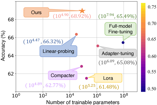
Figure 1: The tradeoff between accuracy and parameter numbers of various model adaptation methods. The results are measured using the vision transformer (ViT-B-224/32) via CLIP pretraining across the average of 20 image classification datasets. Our method places in the topleft corner and achieves the best tradeoff between accuracy and parameter efficiency. The color of points and numbers denote the performance-efficiency (PE) metric (higher is better).

To this end, we ask an essential question: what are the general guidelines one should adopt while adapting large-scale pretrained vision models on the downstream image classification datasets? This work aims to answer the question by building a benchmark for adapting ViTs and proposing a more parameter-efficient model adaptation method. We choose ViTs as the pretrained vision models, which are representative mainstream state-of-the-art (SOTA) models on a wide range of downstream vision tasks. Specifically, we experiment with two off-the-shelf pretrained ViTs in the remainder of this paper: the one via Contrastive Language-Image Pretraining (also known as CLIP) (Radford et al. 2021a), and the one via supervised pretraining (we refer to as Supervised ViT) (Vaswani et al. 2017). In addition to Full-model Fine-tuning and linear-probing, we re-implement several SOTA efficient adaptation methods (Houlsby et al. 2019; Rücklé et al. 2021; Hu et al. 2021; Zaken, Ravfogel, and Goldberg 2021; Li and Liang 2021) (originally proposed for pretrained language models) on vision tasks, and design various new baseline methods for comparison.

Aghajanyan et al. (2020) show that pretrained language models have a low intrinsic dimension and can still learn efficiently despite a low-dimensional reparameterization. Motivated by this observation, we reformulate the task of efficient model adaptation as a subspace training problem. Within this framework, we measure the local intrinsic dimension of each module in ViTs, which reveals that the attention module dominates the training progress. Moreover, we introduce a novel parameter-efficient model adaptation framework named Kronecker Adaptation (KAdaptation), where during adaptation, pretrained weights are frozen, and only the updates to the weights receive gradients. And the weight updates are decomposed to a set of Kronecker products, with the slow weights (Wen, Tran, and Ba 2020) shared across layers and fast weights (Wen, Tran, and Ba 2020) further decomposed into low-rank matrices product to improve parameter efficiency. We apply KAdaptation to attention weights, and it achieves the best average accuracy among efficient model adaptation methods while containing much less trainable parameters, e.g., around 45% parameters of LoRA (Hu et al. 2021) and 0.09% of all the model parameters in CLIP under the few-shot setting.

The contributions of this paper are summarized below:

• We build a benchmark for parameter-efficient model adaptation of ViTs on the image classification task by introducing our new baseline methods and several state-of-the-art efficient model adaptation strategies inspired from the NLP community. To our best knowledge, this is the first empirical study of the efficient model adaptation of Transformers to date that considers pure vision tasks.

• We formulate efficient model adaptation as a subspace training problem. To address it, we define the local intrinsic dimension, based on which we choose submodules — attention modules and we employ the proposed KAdaptation method to decompose the weight updates of attention modules for trainable parameter deduction.

• We experiment on 20 datasets under the few-shot setting and 7 image classification datasets under the full-shot setting. The results demonstrate the effectiveness of our method, achieving the best tradeoff between accuracy and parameter efficiency, as shown in Figure 1.

Related Work

Vision Transformer

Fine-tuning large-scale pretrained ViTs has shown prominent performance for computer vision tasks, such as image classification (Dosovitskiy et al. 2020), object detection (Carion et al. 2020), and etc. Recently, there are also other variants, including hierarchical ViTs with varying resolutions and spatial embeddings (Liu et al. 2021; Dong et al. 2021) been proposed. Undoubtedly, the recent progress of large ViTs posts great demands for developing efficient model adaptation strategies.

Efficient Model Adaptation in NLP

In the natural language processing domain, efficient model adaptation techniques typically involve adding to or modifying a limited number of parameters of the model — limiting the dimension of the optimization problem can prevent catastrophic forgetting (McCloskey and Cohen 1989). Exiting methods are mainly divided into two categories depending on whether new trainable parameters are introduced. Specifically, one is to train a subset of the model parameters, where the common approach is to use a linear probe on top of pretrained features (Radford et al. 2021a). The other alternatives include new parameters in between the network (Li and Liang 2021; Rücklé et al. 2021; Houlsby et al. 2019; Hu et al. 2021; Pfeiffer et al. 2021; Sung, Cho, and Bansal 2022). Nevertheless, these methodologies normally have not been investigated in the computer vision scenario and it is furthermore uncertain if findings from NLP tasks (e.g., question answering (Rajpurkar et al. 2016), natural language understanding (Wang et al. 2018), etc.) can transfer to downstream vision applications. Spurred by those facts, we establish a benchmark to compare these methods and we further advocate our method which can gain a better tradeoff under both the full-shot and few-shot settings.

Efficient Model Adaptation with Subspace Training

Given a large pretrained vision transformer $\mathcal{M}$ with size $|\mathcal{M}|$. Our goal is to develop a parameter-efficient model adaptation technique with trainable parameters $\theta$ of size $d\ll|\mathcal{M}|$, that can attain comparable performance with fine-tuning the whole model. Our ultimate goal is that one could achieve satisfactory results in both efficacy and efficiency without the hassle of fine-tuning the full model.

Subspace Training

A typical neural network contains numerous dense layers that perform matrix multiplication. The weight matrices in these layers can be full-rank. When adapting to a specific task, however, Aghajanyan et al. (2020) show that the pretrained language models have a low intrinsic dimension and can still learn efficiently despite a low-dimensional reparameterization.

Drawing inspiration from their observation and study, we hypothesize that the updates to weights of ViTs during each step in model adaptation also have a low intrinsic rank and develop our method accordingly. The intuition behind our method is to perform subspace training on weight updates. In the de-facto training paradigm of neural network models, the gradient is computed first, followed by gradient steps taken by the optimizer in the entire parameter space $D$. While in subspace training, we instead build a random $d$-dimensional parameter subspace from $\mathcal{M}$, where generally $d\ll|\mathcal{M}|$, and optimize directly in this subspace.

In fact, most current parameter-efficient NLP model adaptation strategies perform subspace training. Given a large pretrained language model $\mathcal{M}$ with size $|\mathcal{M}|$, existing methods either select a submodule from $\mathcal{M}$ or inject an additional module to $\mathcal{M}$. For the parameter vector $\Theta\in\mathbb{R}^{D}$ from this module, they learn a projection $\mathcal{P}$ mapping $\Theta$ into a random $d$-dimensional subspace and perform training in that subspace to minimize computational cost. With this observation, we motivate our study on the efficient model adaptation problem in the principle of subspace training. We approach the problem by addressing two scientific questions: how to choose these submodules and how to make the subspace projection.

The Proposed Kronecker Adaptation

To answer the two fundamental questions of efficient model adaptation, how to choose these submodules and how to make the subspace projection, we propose a novel framework that consists of two corresponding strategies. First, we define the local intrinsic dimension and we choose submodules based on their measured local intrinsic dimensions. Second, we propose a Kronecker Adaptation method to perform the subspace projection on the selected submodules by exploiting parameterized hypercomplex multiplication layers (PHM) (Zhang et al. 2021).

Local Intrinsic Dimension

Measuring the intrinsic dimension of an objective function was first proposed in Li et al. (2018). Aghajanyan et al. (2020) extended it to analyze the quality of pretrained language models. They point out that analyzing model adaptation through the lens of intrinsic dimension offers empirical and theoretical intuitions. Both of them study the intrinsic dimension of the entire model.

Unlike them, we propose to measure the intrinsic dimension of each individual submodule in ViT. We define the intrinsic dimension of the submodule as local intrinsic dimension, to distinguish it from the intrinsic dimension of the whole model. The local intrinsic dimension is indicative of the contribution of each submodule during model adaptation and measuring it will tell us how many free parameters are required to approximate the optimization problem closely. The conventional standard method of measuring the intrinsic dimensionality of an objective (Li et al. 2018) asks for performing grid search over different subspace dimensions $d$, training using standard SGD (Ruder 2016) over the subspace reparameterization, and selecting the smallest $d$ which can produce a satisfactory solution (e.g., 90% of the full training metric). Likewise, we measure the local intrinsic dimension via finding the smallest $d$ for the measured submodule that can reach 90% of the full accuracy.

To this end, we first follow the similar definition in Li et al. (2018) and define $\Theta$ in a subspace in the following way:

$$\Theta=\Theta_{0}+P\theta,$$ (1)

where $\Theta_{0}\in\mathbb{R}^{D}$ is the initial parameter vector of $\Theta$ when the training begins, $P\in\mathbb{R}^{D\times d}$ is the projection matrix generated by the Fastfood transform (Le, Sarlós, and Smola 2014), and $\theta\in\mathbb{R}^{d}$ is the parameter vector in the subspace. Subspace training proceeds by computing gradients with respect to $\theta$ and taking steps in that subspace. By performing experiments with gradually larger values of $d$, we can find the subspace dimension $d_{t}$ at which the performance of the model $\mathcal{M}$ reaches 90% of the full accuracy. We refer to $d_{t}$ the local intrinsic dimension of the measured submodule.

The module with the lowest local intrinsic dimension — attention module is selected. We project them into subspace via our proposed KAdaptation method for the sake of efficient model adaptation. KAdaptation fine-tunes attention weight matrices indirectly by optimizing decomposition matrices of the updates to attention weight matrices. To lower the parameter cost, the decomposition is computed as the sum of Kronecker products while the original matrices remain frozen.

Kronecker Product

The Kronecker product between matrix $\boldsymbol{A}\in\mathbb{R}^{m\times n}$ and $\boldsymbol{B}\in\mathbb{R}^{p\times q}$, denoted by $\boldsymbol{A}\otimes\boldsymbol{B}\in\mathbb{R}^{mp\times nq}$, is mathematically written in the following form:

$$\boldsymbol{A}\otimes\boldsymbol{B}=\left(\begin{array}[]{ccc}a_{11}\boldsymbol{B}&\cdots&a_{1n}\boldsymbol{B}\\ \vdots&\ddots&\vdots\\ a_{m1}\boldsymbol{B}&\cdots&a_{mn}\boldsymbol{B},\end{array}\right)$$ (2)

where $a_{ij}$ shows the element in the $i$-th row and $j$-th column of $\boldsymbol{A}$.

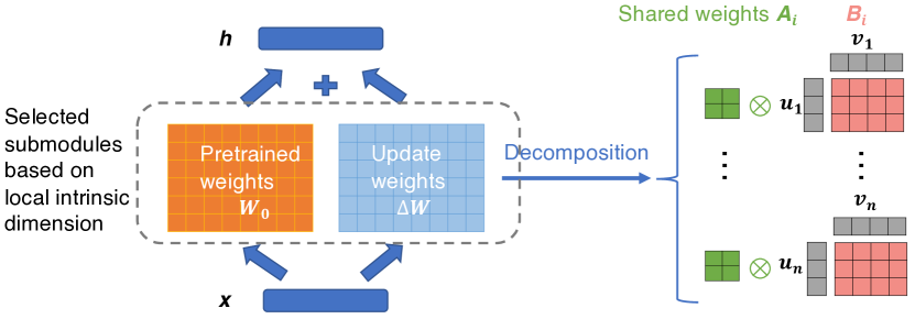
Figure 2: An illustration of KAdaptation. $\boldsymbol{A_{i}}$ denotes the shared weight matrix, with $i\in\{1,\ldots,n\}$. $\boldsymbol{B_{i}}$ is decomposed into two low-rank matrices $\boldsymbol{u}_{\boldsymbol{i}}$ and $\boldsymbol{v}_{\boldsymbol{i}}$. $\boldsymbol{h}$ is the output of the selected ViT submodule. $\boldsymbol{x}$ is the input to the submodule. During model adaptation process, only matrices $\boldsymbol{A_{i}}$, $\boldsymbol{u}_{\boldsymbol{i}}$, and $\boldsymbol{v}_{\boldsymbol{i}}$ receive gradients to improve parameter efficiency.

Kronecker Adaptation

Leveraging the Kronecker product to perform language model compression has been shown to be beneficial in prior works (Tahaei et al. 2021; Edalati et al. 2021). Recently, Zhang et al. (2021) introduces PHM layers, theoretically demonstrating that Kronecker products can help to reduce learnable parameters in language models and maintain performance. Built upon the success of PHM, for an update matrix $\Delta\boldsymbol{W}\in\mathbb{R}^{k\times d}$ in the ViT, we propose the KAdaptation to adapt it into subspace. The illustration is shown in Fig. 2. Mathematically, we compute $\Delta\boldsymbol{W}$ as follows:

$$\Delta\boldsymbol{W}=\sum_{i=1}^{n}\boldsymbol{A}_{\boldsymbol{i}}\otimes\boldsymbol{B}_{\boldsymbol{i}},$$ (3)

where $n$ is the user-defined hyperparameter representing the number of Kronecker products, $\boldsymbol{A}_{\boldsymbol{i}}\in\mathbb{R}^{n\times n}\text{, and }\boldsymbol{B}_{\boldsymbol{i}}\in\mathbb{R}^{\frac{k}{n}\times\frac{d}{n}}$. The new representation of the update weights in Eq. 3 is composed of a sum of $n$ Kronecker products between shared slow weights $\boldsymbol{A}_{i}$ and independent fast weights $\boldsymbol{B}_{i}$, with $i\in\{1,\ldots,n\}$.

Meanwhile, low-rank methods (Aghajanyan, Zettlemoyer, and Gupta 2020; Li et al. 2018; Sainath et al. 2013) have demonstrated that strong performance can be achieved by optimizing models in a low-rank subspace. Similarly, we hypothesize that $\Delta\boldsymbol{W}$ can be effectively adapted by learning transformations in a low-rank subspace to reduce parameter cost further. Therefore, we parameterize $\boldsymbol{B}_{i}\in\mathbb{R}^{\frac{k}{n}\times\frac{d}{n}}$ as low rank and further decompose it into the product of two low-rank matrices $\boldsymbol{u}_{\boldsymbol{i}}\in\mathbb{R}^{\frac{k}{n}\times r}$ and $\boldsymbol{v}_{\boldsymbol{i}}\in\mathbb{R}^{r\times\frac{d}{n}}$, where $r$ is the rank of the matrix. Overall, similar to the low-rank parameterized hypercomplex multiplication layer (LPHM) proposed in Mahabadi, Henderson, and Ruder (2021), the expression of the update matrix $\Delta\boldsymbol{W}$ is then:

$$\Delta\boldsymbol{W}=\sum_{i=1}^{n}\boldsymbol{A}_{\boldsymbol{i}}\otimes\boldsymbol{B}_{\boldsymbol{i}}=\sum_{i=1}^{n}\boldsymbol{A}_{\boldsymbol{i}}\otimes\left(\boldsymbol{u}_{\boldsymbol{i}}\boldsymbol{v}_{\boldsymbol{i}}^{\top}\right).$$ (4)

The number of trainable parameters is now substantially saved. Note that similar to $\boldsymbol{B}_{i}\in\mathbb{R}^{\frac{k}{n}\times\frac{d}{n}}$, the shared slow weights $\boldsymbol{A}_{i}$ can also be further decomposed into the product of low-rank matrices. Additional bias terms can also be applied to the update matrix. We give the analysis of parameter efficiency in the next section.

Analysis of Efficient Model Adaptation Methods

Discussion of State-of-the-art Methods

In what follows, we discuss connections between our method and state-of-the-art parameter-efficient tuning methods on NLP tasks and provide additional insight into the characteristics of our method.

Adapter-tuning (Houlsby et al. 2019)

is the first efficient model adaptation work in the NLP community. It brings in an additional trainable set of modules by adding a trainable bottleneck layer after the feedforward network in each Transformer layer of the pretrained language models. A bottleneck layer consists of a down and up projection pair that shrinks and recovers the size of token hidden states.

Similar to the Adapter-tuning method where they use the bottleneck structure in the additional layer, our method implements low-rank decomposition on the fast rank-one matrices (Wen, Tran, and Ba 2020). The critical functional difference is that our learned weights can be merged with the main weights during inference, thus introducing no latency.

LoRA (Hu et al. 2021)

is another line of work for parameter-efficient language model tuning: it treats the model parameters after fine-tuning as an addition of the pretrained parameters $\Theta_{\text{pretrained }}$ and task-specific differences $\theta_{\text{task }}$, where $\Theta_{\text{pretrained }}$ is fixed and a new subset of model parameters are added on top. Given a pretrained weight matrix $\boldsymbol{W}_{0}\in\mathbb{R}^{d\times k}$, they constrain its update by performing low-rank decomposition: $\boldsymbol{W_{0}}+\Delta\boldsymbol{W}=\boldsymbol{W}_{0}+\boldsymbol{BA}$, where $\boldsymbol{A}\in\mathbb{R}^{r\times k}$, $\boldsymbol{B}\in\mathbb{R}^{d\times r}$, and the rank $r\ll\min(d,k)$. By doing this, the weight matrices are split into two parts, where during training, $\boldsymbol{W}_{0}$ is frozen and receives no gradient updates, while only $\boldsymbol{A}$ and $\boldsymbol{B}$ contain trainable parameters.

Our work differs from LoRA mainly in that we decompose weight updates to a set of Kronecker product decomposition. The decomposed slow weight are shared across layers, further reducing the parameter cost.

Compacter (Mahabadi, Henderson, and Ruder 2021)

inserts task-specific weight matrices into weights of pretrained models. Each Compacter weight matrix is computed as the sum of Kronecker products between shared slow weights and fast matrices defined per Compacter layer.

In a similar vein to Compacter, we also leverage the Kronecker product in our method to reduce parameter cost further. Yet, apart from application domains, our method fundamentally differs from Adapter/Compacter based methods in that: first, our method brings in no additional layer and introduces no latency; Second, our method first selects submodules by measuring the local intrinsic dimension and then performs the KAdaptation over the update weights to selected submodules; Third, during adaptation, only updates to the weights of selected submodules receive gradients and tuned, while pretrained weights are always fixed.

Method	#Params	Complexity
Adapter-tuning	$4Lkd$	$\mathcal{O}\left(kd\right)$
LoRA	$2Lrd_{model}$	$\mathcal{O}\left(rd_{model}\right)$
Compacter	$4L(\frac{k}{n}+\frac{d}{n})+n^{3}$	$\mathcal{O}\left(\frac{k+d}{n}\right)$
KAdaptation	$2L(\frac{d_{model}}{n}+\frac{r}{n})+n^{3}$	$\mathcal{O}\left(\frac{r+d_{model}}{n}\right)$

Table 1: Parameter count in Adapter-tuning, LoRA, Compacter, and KAdaptation. $L$ is the number of layers in the Transformer. $k$ is the size of the input dimension to the Adapter layer. $d$ is the bottleneck dimension in the Adapter layer. $d_{model}$ is the Transformer hidden size. $r$ denotes the rank in the low-rank decomposition step. $n$ is the number of Kronecker products usually very small.

Analysis of Parameter Efficiency

We analyze the parameter-efficiency of our KAdaptation and other model adaptation methods as below:

Adapter-tuning

In the standard setting, two Adapters are added per layer of a Transformer model (Baevski and Auli 2019). Each Adapter layer consists of $2\times k\times d$ parameters for the down and up-projection matrices, where $k$ is the size of the input dimension and $d$ is the Adapter’s bottleneck dimension. The total number of parameters for Adapters for a $L-$layer Transformer is, $|\Theta|=2\times L\times 2\times k\times d$s.

LoRA

LoRA adds trainable pairs of rank decomposition matrices to existing weight matrices. The number of trainable parameters is determined by the rank $r$: $|\Theta|=2\times L\times d_{\text{model }}\times r$, where $d_{\text{model }}$ is Transformer hidden size.

Compacter

Compacter shares the trained weight matrices $\left\{\boldsymbol{A}_{\boldsymbol{i}}\right\}_{i=1}^{n}$ consisting of $n^{3}$ parameters across all layers, where $n$ is the number of Kronecker products. Compacter also has two rank-one weights for each Adapter layer consisting of $\frac{k}{n}+\frac{d}{n}$ parameters, where the Adapter layers are of size $k\times d$, resulting in a total of $2\times\left(\frac{k}{n}+\frac{d}{n}\right)$ parameters for down and up-projection weights. Therefore, the total number of parameters of Compacter is $4\times L\times\left(\frac{k}{n}+\frac{d}{n}\right)+n^{3}$ for a Transformer with $L$ layers in the encoder and decoder.

Our Approach

we analyze the parameter efficiency of our approach under the scenario where we decompose the updates to weights into a sum of Kronecker products first and then further perform low-rank decomposition for the fast weights. The total number of parameters in this scenario will be: $2\times L\times\left(\frac{r+d_{model}}{n}\right)+n^{3}$.

The overall comparison of parameter counts is shown in Table 1. Our method has a complexity of $\mathcal{O}\left(\frac{r+d_{model}}{n}\right)$ with $r$ being a small integer. Our approach greatly reduces the number of parameters. The exact numbers of trainable parameters are present in Table 3.

Experiments

Method	Caltech101	CIFAR10	CIFAR100	Country211	DTD	EuroSat	FER2013	FGVCAircraft	Food101	GTSRB	HatefulMemes	KittiDistance	MNIST	Flowers102	OxfordPets	PatchCamelyon	SST2	RESISC45	StanfordCars	VOC2007	Ave Acc ($\uparrow$)	#Params ($\downarrow$)	PE ($\uparrow$)
Fine-tuning	87.64	91.11	71.52	15.75	54.36	85.24	52.72	26.22	83.28	74.05	55.64	39.15	65.55	80.55	87.31	64.92	59.09	75.61	57.21	82.95	65.49	87,878,739	0.498
Linear-probing	90.96	90.35	67.31	17.36	62.04	72.95	51.91	29.52	83.82	56.47	55.83	40.37	77.50	92.29	88.03	59.00	59.36	78.10	68.30	84.99	66.32	29,523	0.663
Adapter-tuning	90.18	90.14	73.57	16.83	57.13	67.97	41.76	30.52	83.58	58.50	48.91	37.18	80.34	90.78	86.52	59.92	58.70	79.22	67.68	82.22	65.08	1,237,587	0.647
LoRA	87.64	90.52	69.69	17.12	50.16	74.03	51.04	20.01	83.76	42.96	55.88	48.05	61.36	74.28	85.49	63.20	57.04	62.09	54.89	80.33	61.48	176,979	0.614
Compacter	89.02	79.96	44.33	28.22	52.93	50.48	35.46	41.13	78.28	66.90	47.60	57.72	85.82	88.29	79.23	61.83	64.22	63.76	64.79	75.84	62.79	77,907	0.628
KAdaptation	88.96	90.03	73.92	17.53	63.97	76.25	47.45	30.04	84.38	80.71	55.86	42.29	85.20	93.19	89.05	63.39	59.18	79.96	70.21	84.49	68.92	79,699	0.689

Table 2: The averaged 5-shot experimental result comparison on 20 datasets from ELEVATER benchmark (Li et al. 2022b) in terms of accuracy (%) and number of trainable parameters (#Params) across random seeds of {$0$, $1$, $2$}. The vision transformer (ViT-B-224/32) via CLIP pretraining is evaluated. Our method achieves the best tradeoff between accuracy and parameter efficiency: it obtains the best average accuracy among all efficient model adaptation methods, while updating only 0.09% of the model parameters in CLIP. We color each accuracy value as the best and second best: the same hereinafter.

Datasets

For few-shot benchmark experiments, we conduct experiments on 20 image classification datasets from the ELEVATER benchmark (Li et al. 2022b) on four Quadro RTX A6000 GPUs. Detailed dataset statistics are given in the supplementary material. For full-shot experiments, we summarize the results by computing the average performance on CIFAR10 (Krizhevsky, Hinton et al. 2009), CIFAR100 (Krizhevsky, Hinton et al. 2009), SUN397 (Xiao et al. 2010), DTD (Cimpoi et al. 2014a), STL10 (Coates, Ng, and Lee 2011), FGVCAircraft (Maji et al. 2013a), and FER2013 (Goodfellow et al. 2013a). We use the official split for each of these datasets.

Implementation Details

For benchmark experiments, we use the SGD (Ruder 2016) optimizer with the learning rate and weight decay being automatically searched for all methods so that these two hyperparameters have the optimum combination. We borrow the automatic hyper-parameter tuning toolkit from Li et al. (2022b). Training epochs are set via grid search. We test two pretrained $12$-layer ViTs: the one using ViT-B-224/32 via unsupervised pretraining (CLIP) and the one using ViT-B-224/16 via supervised pretraining (Supervised ViT).

For intrinsic dimension experiments, we use the AdamW (Kingma and Ba 2014) as the optimizer, with the weight decay of $10^{-8}$, learning rate of $10^{-5}$, and batch size of 32 following the setting in Li et al. (2018). The Fastfood transform (Le, Sarlós, and Smola 2014) is applied to the attention and multi-layer perceptron (MLP) module in the first layer of Supervised ViT, respectively. The dimension $d$ is measured from $0-2000$ in both scenarios. Each model is fine-tuned for 300 epochs.

Baselines

We test the baselines below. Unless otherwise specified, the task-specific classification layer and added parameters are tuned while the pretrained ViTs are frozen.

First are commonly-used model adaptation methods for vision models.

• Full-model Fine-tuning: fine-tunes all model parameters.

• Linear-probing: only tune the task-specific classification layer.

The second types are SOTA methods borrowed from the NLP community.

• BitFit (Zaken, Ravfogel, and Goldberg 2021): freezes all ViT parameters except for the bias terms and the task-specific classification layer.

• Adapter-tuning (Houlsby et al. 2019): two Adapters are added and tuned in each Transformer layer.

• AdapterDrop (Rücklé et al. 2021): only keep Adapters from the last Transformer layer.

• LoRA (Hu et al. 2021): apply LoRA to $\boldsymbol{W}_{q}$ and $\boldsymbol{W}_{v}$ matrices in the attention module and tune the low-rank decomposition matrices.

• Compacter (Mahabadi, Henderson, and Ruder 2021): we experiment with $n=4$.

The third types are new baseline methods we developed.

• Transformer-probing: an additional trainable Transformer block is stacked before the task-specific classification layer and tuned.

• LoRA-Fix: the matrix $\boldsymbol{A}$ in LoRA (Hu et al. 2021) is fixed and only the matrix $\boldsymbol{B}$ is tuned.

• LayerNorm Tuning: the layer norm layers are tuned.

• Attention Tuning: the attention layers are tuned.

• LePE Tuning (Dong et al. 2021): locally-enhanced positional encoding (LePE) is added to the ViT and tuned. We implement it by the depthwise convolution operator (Chollet 2017) on the matrix $\boldsymbol{V}$ in the attention layer: $\operatorname{Attention}(\boldsymbol{Q},\boldsymbol{K},\boldsymbol{V})=\operatorname{SoftMax}\left(\boldsymbol{Q}\boldsymbol{K}^{T}/\sqrt{d}\right)\boldsymbol{V}+\operatorname{DWConv}(\boldsymbol{V}).$

• Relative Position Bias (RPB) Tuning (Liu et al. 2021): an additional relative position bias term $\boldsymbol{B}$ is included in computing self-attention in the ViT and tuned: $\operatorname{Attention}(\boldsymbol{Q},\boldsymbol{K},\boldsymbol{V})=\operatorname{SoftMax}\left(\boldsymbol{Q}\boldsymbol{K}^{T}/\sqrt{d}+\boldsymbol{B}\right)\boldsymbol{V}.$

LayerNorm Tuning, Attention Tuning, and BitFit shed light on which parameters in ViT matter more during model adaptation. Among all modules in ViT, multi-layer perceptron (MLP) tuning is not considered a baseline because it is prohibitively costly compared to others. Given that the special structure of ViT and its variants, e.g., depthwise convolution operator and relative position bias, are different from the general transformers in natural language processing, we actually made the first step towards parameter-efficient model adaptation for the ViT via LePE Tuning and Relative Position Bias Tuning.

Results and Analysis

Metric with performance-efficiency trade-off

To better compare different methods with a single number that considers both prediction accuracy and parameter-efficiency, we resort to the performance-efficiency (PE) metric defined in Li et al. (2022a):

$$\text{PE}=\text{score}*\exp\left(-\log_{10}(\text{\# trainable-parameters }/M_{0}+1)\right)$$

where score is the prediction accuracy, while # trainable-parameters is the number of updated parameters in the model adaptation stage, and $M_{0}$ is the normalization constant. $M_{0}$ is set to $10^{8}$ because most existing vision backbone model size are in this magnitude, for example, ViT-Base (80M parameters).

The experimental results of measured average accuracy across the 20 datasets in the low-data regime and under the 5-shot setting using random seeds of $0$, $1$, and $2$ are shown in Table 2. As observed, the parameter cost of linear-probing is the lowest while that of full-model fine-tuning is the highest. Our method has the highest average accuracy and remains the ideal approach with the optimum tradeoff: our method has much less trainable parameters than other adaptation methods — the second lowest and is only higher than Linear-probing. From the performance-efficiency trade-off metric, it can also be seen that ours has the highest PE.

To further compare our method with SOTA methods for NLP models and more baselines, we investigate the performance of adaptation approaches in the full-data regime and test under the full-shot setting. The results across the seven datasets are shown in Table 3. In our analytical experiments, we first observe that Full-model Fine-tuning has the highest accuracy in both scenarios, serving as a performance upper bound. Second, different efficient model adaptation methods exhibit diverse characteristics and perform differently on the same task. Third, the results from CLIP are mostly consistent with the results from Supervised ViT. This suggests that the pretraining strategy may not affect the selection of downstream model adaptation strategy much. Fourth, previous methods such as Adapter-tuning (Houlsby et al. 2019) and LoRA (Hu et al. 2021) are still effective, and their accuracy is substantially higher than naive baselines, including BitFit and Attention-tuning regardless of the pretrained checkpoint. Fifth, among naive baselines where only submodules or task-specific classification heads are tuned, tuning the parameters of the attention layer turns out to be a surprisingly effective approach even compared to some SOTA methods, though its parameter cost is significantly higher. This further validates the effectiveness of our method by applying KAdaptation to attention weights. Finally, our method outperforms all the SOTA methods borrowed from the NLP community as well as their variants in both scenarios.

Furthermore, the average number of trainable parameters across seven datasets is also shown in Table 3. As can be seen, our KAdaptation method contains the lowest parameter cost compared with other SOTA methods. This phenomenon is obviously noticeable when compared with Full-model Fine-tuning, where our method takes less than 0.14% of trainable parameters of end-to-end Full-model Fine-tuning but it is capable of achieving comparable performance.

Method	CLIP									Supervised ViT
	CIFAR10	CIFAR100	SUN397	DTD	FER2013	FGVCAircraft	STL10	Average ($\uparrow$)	#Params ($\downarrow$)	CIFAR10	CIFAR100	SUN397	DTD	FER2013	FGVCAircraft	STL10	Average ($\uparrow$)	#Params ($\downarrow$)
Commonly-used model adaptation methods for vision models
Full-model Fine-tuning	97.7	85.4	73.8	79.0	69.8	59.0	99.7	80.6	87,897,654	99.0	92.4	75.0	72.4	68.2	52.6	99.6	79.9	86,630,561
Linear-probing	94.8	80.1	72.4	75.4	67.3	49.7	98.4	76.9	49,175	96.3	87.7	70.1	72.7	60.1	45.0	98.7	75.8	49,175
SOTA methods for NLP models
BitFit	92.1	76.0	70.8	75.9	68.0	54.5	98.8	76.6	179,049	92.3	81.0	71.8	72.6	60.4	45.9	99.0	74.7	358,741
Adapter-tuning	94.7	81.4	77.1	78.0	68.4	55.3	99.0	79.1	1,242,843	98.4	90.6	74.2	71.0	63.4	52.4	99.3	78.5	1,505,654
AdapterDrop	93.3	78.3	71.4	77.1	67.1	51.3	98.0	76.6	91,487	96.8	88.4	72.3	70.2	46.9	35.6	99.6	72.8	174,646
LoRA	95.1	78.1	80.8	78.1	67.7	55.8	99.2	79.3	147,236	98.7	90.6	73.6	70.4	62.7	54.9	99.4	78.6	219,601
Baseline methods developed in this work
Transformer-probing	95.6	80.1	74.3	75.9	67.6	50.9	98.5	77.6	3,198,999	96.5	86.9	76.7	72.0	60.7	45.5	99.0	76.8	3,198,999
LoRA-Fix	92.5	77.1	60.0	77.7	65.5	44.4	88.6	72.3	98,481	96.2	88.3	72.0	65.5	53.4	51.7	99.0	75.2	148,704
LayerNorm Tuning	82.5	76.6	66.7	72.4	61.0	37.6	99.1	70.8	52,405	92.2	71.7	72.0	69.0	52.7	51.0	98.8	72.5	75,413
Attention Tuning	96.8	81.8	73.1	75.0	62.2	54.2	97.6	77.2	41,005,636	93.9	85.7	73.8	69.2	55.2	51.9	99.2	75.6	28,405,278
LePE Tuning	95.1	78.9	68.0	75.4	65.2	54.0	98.0	76.4	112,556	93.7	90.8	73.2	69.8	60.0	49.3	99.1	76.6	167,225
RPB Tuning	94.7	77.1	68.4	75.2	65.1	54.1	97.9	76.1	66,768	96.7	87.0	72.4	70.4	50.9	51.4	98.9	75.4	145,920
KAdaptation	95.9	84.8	74.0	78.1	69.0	56.0	99.2	79.6	80,726	97.9	91.2	75.1	71.4	63.8	55.5	99.4	79.2	114,079

Table 3: Experimental result comparison on CIFAR10 (Krizhevsky, Hinton et al. 2009), CIFAR100 (Krizhevsky, Hinton et al. 2009), SUN397 (Xiao et al. 2010), DTD (Cimpoi et al. 2014a), STL10 (Coates, Ng, and Lee 2011), FGVCAircraft (Maji et al. 2013a), and FER2013 (Goodfellow et al. 2013a) datasets in terms of accuracy (%) and number of trainable parameters (#Params).

To further validate the efficiency of our proposed method, in addition to parameter costs, we perform additional evaluation on memory footprint and inference time. We compare the per-sample memory usage of each method in Table 4. Our method reduces memory overhead by $-86.0$% compared to Full-model Fine-tuning and is in the same order of magnitude as other efficient model adaptation methods. We compare the inference time cost per batch in Table 4 as well. On average, our method costs $6.93$s per batch, the same as the vanilla ViT and LoRA, while Adapter-tuning costs $12.97$s and Compacter takes $14.90$s. Our method is the most efficient. It’s within expectation as our method does not bring any additional layer to the original ViT, suffering from no inference latency.

Method	Average Accuracy ($\uparrow$)	Inference time ($\downarrow$)	Memory ($\downarrow$)
Full-model Fine-tuning	79.9	6.93	421.5
Linear-probing	75.8	6.93	27.1
Adapter-tuning	78.5	12.97	70.2
LoRA	78.6	6.93	56.0
Compacter	78.6	14.90	70.0
KAdaptation	79.2	6.93	59.1

Table 4: Average accuracy (%), average inference time/throughput (s) per batch, and average peak memory (MB) for each method. Our method is time-efficient, and our memory footprint is in the same order of magnitude as other efficient model adaptation methods and much less than Full-model Fine-tuning.

Local Intrinsic Dimension

Local intrinsic dimension (Li et al. 2018) informs us of the importance of each module in the ViT and we select submodules to perform KAdaptation based on the measurement results of the local intrinsic dimension. We measure the local intrinsic dimension of the two fundamental architectural components in the ViT — the MLP module and the attention module. We use the remarkable Fastfood transform (Le, Sarlós, and Smola 2014) to do the projection. The accuracy results averaged across $\{1,6,12\}$-th ViT layers are shown in Fig. 3. As a substantiating point to performing Kronecker Adaptation on attention layers, we can see the attention module has a lower intrinsic dimension than the MLP module (300 vs. 575).

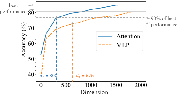
Figure 3: Validation Accuracy vs. Subspace Dimension $d$ of MLP and the attention module for Supervised ViT on CIFAR100. The local intrinsic dimension $d_{t}$ of the attention module is lower than that of the MLP.

Method	Average Accuracy
Adapters on attention layer	54.1
Standard Adapter-tuning	87.7
KAdaptation to MLP	86.6
KAdaptation	88.1

Table 5: KAdaptation and Adapter-tuning ablation experiments with Supervised ViT on CIFAR10 (Krizhevsky, Hinton et al. 2009), CIFAR100 (Krizhevsky, Hinton et al. 2009), and SUN397 (Xiao et al. 2010). We report the average accuracy (%) across the three datasets.

Ablation Studies

We ablate our method and Adapter-tuning using the settings in Table 3. As can be seen in Table 5, several intriguing properties are observed. First, applying KAdaptation to MLP modules performs worse than the original method where we apply KAdaptation to attention modules. This phenomenon is consistent with our findings from naive baseline experiments and intrinsic dimension experiments. Second, we test another variant of Adapter-tuning. Instead of inserting two Adapters after the attention and feedforward modules respectively following Houlsby et al. (2019), we add Adapters in the attention layers. It can be observed that the standard Adapter-tuning outperforms this variance, indicating the effectiveness of the vanilla Adapter-tuning when it is adapted to vision tasks.

Conclusion

In this paper, we conduct the first comprehensive comparison of efficient model adaptation on the image classification tasks using vision transformers. We also propose a better parameter-efficient model adaptation strategy in the principle of subspace training and parameterized hypercomplex multiplication, which achieves the best tradeoff between accuracy and parameter efficiency. We release a benchmark by providing the implementation of all the methods studied in this paper, which could be directly used in developing future efficient model adaptation strategies and will hopefully facilitate research in this area. Looking into the future, we plan to explore the generalization of our method to other tasks, especially in the vision-and-language domain.

Appendix A Detailed Dataset Statistics

For the few-shot setting, we test on Caltech101 (Fei-Fei, Fergus, and Perona 2004), CIFAR10 (Krizhevsky, Hinton et al. 2009), CIFAR100 (Krizhevsky, Hinton et al. 2009), Country211 (Radford et al. 2021b), DTD (Cimpoi et al. 2014b), EuroSat (Helber et al. 2019), FER2013 (Goodfellow et al. 2013b), FGVCAircraft (Maji et al. 2013b), Food101 (Bossard, Guillaumin, and Gool 2014), GTSRB (Stallkamp et al. 2011), HatefulMemes (Kiela et al. 2020), KittiDistanc (Fritsch, Kuehnl, and Geiger 2013), MNIST (Deng 2012), Flowers102 (Nilsback and Zisserman 2008), OxfordPets (Parkhi et al. 2012), PatchCamelyon (Veeling et al. 2018), SST2 (Radford et al. 2021b), RESISC45 (Cheng, Han, and Lu 2017), StanfordCars (Krause et al. 2013), and VOC2007 (Everingham et al. 2010) using the vision transformer (ViT-B-224/32) via Contrastive Language-Image Pretraining (also known as CLIP). In Table 6, we list the basic statistics of 20 image classification datasets used in our few-shot setting experiments.

For the full-shot setting, we use the seven datasets mentioned in the main paper: CIFAR10 (Krizhevsky, Hinton et al. 2009), CIFAR100 (Krizhevsky, Hinton et al. 2009), SUN397 (Xiao et al. 2010), DTD (Cimpoi et al. 2014a), STL10 (Coates, Ng, and Lee 2011), FGVCAircraft (Maji et al. 2013a), and FER2013 (Goodfellow et al. 2013a).

Dataset	#Concepts	Train size	Test size	Evaluation metric
Hateful Memes (Kiela et al. 2020)	2	8,500	500	ROC AUC
PatchCamelyon (Veeling et al. 2018)	2	262,144	32,768	Accuracy
Rendered-SST2 (Radford et al. 2021b)	2	6,920	1,821	Accuracy
KITTI Distance (Fritsch, Kuehnl, and Geiger 2013)	4	6,347	711	Accuracy
FER 2013 (Goodfellow et al. 2013b)	7	28,709	3,589	Accuracy
CIFAR10 (Krizhevsky, Hinton et al. 2009)	10	50,000	10,000	Accuracy
EuroSAT (Helber et al. 2019)	10	5,000	5,000	Accuracy
MNIST (Deng 2012)	10	60,000	10,000	Accuracy
VOC 2007 Classification (Everingham et al. 2010)	20	2,501	4,952	11-point mAP
Oxford-IIIT Pets (Parkhi et al. 2012)	37	3,680	3,669	Mean-per-class
GTSRB (Stallkamp et al. 2011)	43	26,640	12,630	Accuracy
Resisc-45 (Cheng, Han, and Lu 2017)	45	3,150	25,200	Accuracy
Describable Textures (Cimpoi et al. 2014b)	47	1,880	1,880	Accuracy
CIFAR100 (Krizhevsky, Hinton et al. 2009)	100	50,000	10,000	Accuracy
FGVC Aircraft (variants) (Maji et al. 2013b)	100	3,334	3,333	Mean-per-class
Food-101 (Bossard, Guillaumin, and Gool 2014)	101	75,750	25,250	Accuracy
Caltech101 (Fei-Fei, Fergus, and Perona 2004)	102	3,060	6,084	Mean-per-class
Oxford Flowers 102 (Nilsback and Zisserman 2008)	102	1,020	6,149	Mean-per-class
Stanford Cars (Krause et al. 2013)	196	8,144	8,041	Accuracy
Country-211 (Radford et al. 2021b)	211	31,650	21,100	Accuracy
Total	2151	1,919,596	242,677	–

Table 6: Statistics of 21 datasets used in few-shot image classification experiments.

Name	Value	Description
Optimizer	SGD	-
Learning rate	$10^{-6}$-$10^{6}$	Automatically searched for each dataset
Weight decay	-	Automatically searched for each dataset
Max epoch	50	-
Batch size	32	-

Table 7: Hyperparameter settings for benchmark experiments under the few-shot setting.

Appendix B Hyperparameter Settings

The overall hyperparameter settings for benchmark experiments under the few-shot setting are specified in Table 7. We repeat experiments for three different random seeds of $\{0,1,2\}$. The learning rate and weight decay are automatically searched so that these two hyperparameters will always have the optimum combination. The number of seaching epochs is set to 10. The number of training epochs is set to 50. For the method-specific hyperparameter settings, for all Adapter-based methods (Houlsby et al. 2019), we experiment with Adapters of bottleneck size of 64; For Compacter (Mahabadi, Henderson, and Ruder 2021), we experiment with the number of Kronecker products $n=4$; For LoRA (Hu et al. 2021), we follow the same setting in the original paper; In our KAdaptation method, we set the user-defined hyperparameter $n\in\mathbb{Z}>0$, which is the number of Kronecker products, by performing the grid search from $\{4,32,64\}$ and choosing the best one. We report the model performing the best with $n=32$.

The overall hyperparameter settings for benchmark experiments under the full-shot setting are specified in Table 8. For each method, we set the batch size to 64. All experiments are performed with the same random seed. The optimum number of training epochs is set by grid search in the range of {100, 200, 400}.

Name	Value	Description
Optimizer	SGD	-
Learning rate	$10^{-6}$-$10^{6}$	Automatically searched for each dataset
Weight decay	-	Automatically searched for each dataset
Max epoch	100-400	Grid search
Batch size	64	-

Table 8: Hyperparameter settings for benchmark experiments under the full-shot setting.

Appendix C Additional Related Works

Transformers

Transformer (Vaswani et al. 2017) is a sequence-to-sequence architecture that makes heavy use of self-attention mechanisms to replace the recurrence and convolution operations. It is initially used for machine translation (Bahdanau, Cho, and Bengio 2014) and has shown outstanding performance in a wide range of natural language processing (NLP) tasks, including reading comprehension (Dai et al. 2020), question answering (Min et al. 2019), vision-and-language tasks (Li et al. 2020), etc. Since Radford et al. (2019) first applied a stack of Transformer decoders to autoregressive language modeling, fine-tuning Transformer-based language models has dominated NLP, achieving state-of-the-art performance in many tasks. Meanwhile, fine-tuning large-scale pretrained ViTs has shown prominent performance for computer vision tasks, such as image classification (Dosovitskiy et al. 2020), object detection (Carion et al. 2020), etc. Recently, there are also other variants, including hierarchical ViTs with varying resolutions and spatial embeddings (Liu et al. 2021; Dong et al. 2021) been proposed. Beyond doubt, the recent progress of large Transformer-alike models posts great demands for developing efficient model adaptation strategies.

Pretraining

Pretraining in NLP (Liu et al. 2019; Devlin et al. 2018), has achieved state-of-the-art performances in many downstream tasks (Thongtan and Phienthrakul 2019; White et al. 2017). It is widely deemed that adapting models pretrained on general domain data (Devlin et al. 2018; Radford et al. 2019) to downstream datasets could provide a substantial performance gain compared to training on task-specific data directly. In computer vision, adapting pretrained models, e.g. (Simonyan and Zisserman 2014; He et al. 2016; Dosovitskiy et al. 2020), has come to the forefront of deep learning techniques due to its success in downstream tasks (Ren et al. 2015; Lee et al. 2018) that can substantially outperform tuning models with random initialization. In this paper, we will mainly focus on the parameter-efficient model adaptation of pretrained ViT on the image classification task.

References

- Aghajanyan, Zettlemoyer, and Gupta (2020) Aghajanyan, A.; Zettlemoyer, L.; and Gupta, S. 2020. Intrinsic Dimensionality Explains the Effectiveness of Language Model Fine-Tuning. arXiv:2012.13255 [cs].
- Baevski and Auli (2019) Baevski, A.; and Auli, M. 2019. Adaptive Input Representations for Neural Language Modeling. In ICLR.
- Bahdanau, Cho, and Bengio (2014) Bahdanau, D.; Cho, K.; and Bengio, Y. 2014. Neural machine translation by jointly learning to align and translate. arXiv preprint arXiv:1409.0473.
- Bossard, Guillaumin, and Gool (2014) Bossard, L.; Guillaumin, M.; and Gool, L. V. 2014. Food-101–mining discriminative components with random forests. In ECCV.
- Carion et al. (2020) Carion, N.; Massa, F.; Synnaeve, G.; Usunier, N.; Kirillov, A.; and Zagoruyko, S. 2020. End-to-end object detection with transformers. In European Conference on Computer Vision, 213–229. Springer.
- Cheng, Han, and Lu (2017) Cheng, G.; Han, J.; and Lu, X. 2017. Remote sensing image scene classification: Benchmark and state of the art. Proceedings of the IEEE.
- Chollet (2017) Chollet, F. 2017. Xception: Deep learning with depthwise separable convolutions. In Proceedings of the IEEE conference on computer vision and pattern recognition, 1251–1258.
- Cimpoi et al. (2014a) Cimpoi, M.; Maji, S.; Kokkinos, I.; Mohamed, S.; ; and Vedaldi, A. 2014a. Describing Textures in the Wild. In Proceedings of the IEEE Conf. on Computer Vision and Pattern Recognition (CVPR).
- Cimpoi et al. (2014b) Cimpoi, M.; Maji, S.; Kokkinos, I.; Mohamed, S.; and Vedaldi, A. 2014b. Describing textures in the wild. In CVPR.
- Coates, Ng, and Lee (2011) Coates, A.; Ng, A.; and Lee, H. 2011. An analysis of single-layer networks in unsupervised feature learning. In Proceedings of the fourteenth international conference on artificial intelligence and statistics, 215–223. JMLR Workshop and Conference Proceedings.
- Dai et al. (2020) Dai, Z.; Lai, G.; Yang, Y.; and Le, Q. V. 2020. Funnel-transformer: Filtering out sequential redundancy for efficient language processing. arXiv preprint arXiv:2006.03236.
- Deng (2012) Deng, L. 2012. The MNIST database of handwritten digit images for machine learning research. IEEE signal processing magazine.
- Devlin et al. (2018) Devlin, J.; Chang, M.-W.; Lee, K.; and Toutanova, K. 2018. Bert: Pre-training of deep bidirectional transformers for language understanding. arXiv preprint arXiv:1810.04805.
- Dong et al. (2021) Dong, X.; Bao, J.; Chen, D.; Zhang, W.; Yu, N.; Yuan, L.; Chen, D.; and Guo, B. 2021. Cswin transformer: A general vision transformer backbone with cross-shaped windows. arXiv preprint arXiv:2107.00652.
- Dosovitskiy et al. (2020) Dosovitskiy, A.; Beyer, L.; Kolesnikov, A.; Weissenborn, D.; Zhai, X.; Unterthiner, T.; Dehghani, M.; Minderer, M.; Heigold, G.; Gelly, S.; et al. 2020. An image is worth 16x16 words: Transformers for image recognition at scale. arXiv preprint arXiv:2010.11929.
- Edalati et al. (2021) Edalati, A.; Tahaei, M.; Rashid, A.; Nia, V. P.; Clark, J. J.; and Rezagholizadeh, M. 2021. Kronecker decomposition for gpt compression. arXiv preprint arXiv:2110.08152.
- Everingham et al. (2010) Everingham, M.; Van Gool, L.; Williams, C. K.; Winn, J.; and Zisserman, A. 2010. The pascal visual object classes (VOC) challenge. IJCV.
- Fei-Fei, Fergus, and Perona (2004) Fei-Fei, L.; Fergus, R.; and Perona, P. 2004. Learning generative visual models from few training examples: An incremental Bayesian approach tested on 101 object categories. In CVPR workshop.
- Fritsch, Kuehnl, and Geiger (2013) Fritsch, J.; Kuehnl, T.; and Geiger, A. 2013. A new performance measure and evaluation benchmark for road detection algorithms. In ITSC. IEEE.
- Goodfellow et al. (2013a) Goodfellow, I. J.; Erhan, D.; Carrier, P. L.; Courville, A.; Mirza, M.; Hamner, B.; Cukierski, W.; Tang, Y.; Thaler, D.; Lee, D.-H.; et al. 2013a. Challenges in representation learning: A report on three machine learning contests. In International conference on neural information processing, 117–124. Springer.
- Goodfellow et al. (2013b) Goodfellow, I. J.; Erhan, D.; Carrier, P. L.; Courville, A.; Mirza, M.; Hamner, B.; Cukierski, W.; Tang, Y.; Thaler, D.; Lee, D.-H.; et al. 2013b. Challenges in representation learning: A report on three machine learning contests. In International conference on neural information processing, 117–124. Springer.
- He et al. (2021) He, J.; Zhou, C.; Ma, X.; Berg-Kirkpatrick, T.; and Neubig, G. 2021. Towards a unified view of parameter-efficient transfer learning. arXiv preprint arXiv:2110.04366.
- He et al. (2016) He, K.; Zhang, X.; Ren, S.; and Sun, J. 2016. Deep residual learning for image recognition. In CVPR.
- Helber et al. (2019) Helber, P.; Bischke, B.; Dengel, A.; and Borth, D. 2019. EuroSat: A novel dataset and deep learning benchmark for land use and land cover classification. IEEE Journal of Selected Topics in Applied Earth Observations and Remote Sensing.
- Houlsby et al. (2019) Houlsby, N.; Giurgiu, A.; Jastrzebski, S.; Morrone, B.; de Laroussilhe, Q.; Gesmundo, A.; Attariyan, M.; and Gelly, S. 2019. Parameter-Efficient Transfer Learning for NLP. arXiv:1902.00751 [cs, stat].
- Hu et al. (2021) Hu, E. J.; Shen, Y.; Wallis, P.; Allen-Zhu, Z.; Li, Y.; Wang, S.; Wang, L.; and Chen, W. 2021. LoRA: Low-Rank Adaptation of Large Language Models. arXiv:2106.09685 [cs].
- Kiela et al. (2020) Kiela, D.; Firooz, H.; Mohan, A.; Goswami, V.; Singh, A.; Ringshia, P.; and Testuggine, D. 2020. The hateful memes challenge: Detecting hate speech in multimodal memes. NeurIPS.
- Kingma and Ba (2014) Kingma, D.; and Ba, J. 2014. Adam: A Method for Stochastic Optimization. International Conference on Learning Representations.
- Krause et al. (2013) Krause, J.; Stark, M.; Deng, J.; and Fei-Fei, L. 2013. 3d object representations for fine-grained categorization. In ICCV workshops.
- Krizhevsky, Hinton et al. (2009) Krizhevsky, A.; Hinton, G.; et al. 2009. Learning multiple layers of features from tiny images.
- Le, Sarlós, and Smola (2014) Le, Q. V.; Sarlós, T.; and Smola, A. J. 2014. Fastfood: Approximate kernel expansions in loglinear time. arXiv preprint arXiv:1408.3060.
- Lee et al. (2018) Lee, K.-H.; Chen, X.; Hua, G.; Hu, H.; and He, X. 2018. Stacked cross attention for image-text matching. In Proceedings of the European Conference on Computer Vision (ECCV), 201–216.
- Li et al. (2018) Li, C.; Farkhoor, H.; Liu, R.; and Yosinski, J. 2018. Measuring the Intrinsic Dimension of Objective Landscapes. arXiv:1804.08838 [cs, stat].
- Li et al. (2022a) Li, C.; Liu, H.; Li, L. H.; Zhang, P.; Aneja, J.; Yang, J.; Jin, P.; Lee, Y. J.; Hu, H.; Liu, Z.; and Gao, J. 2022a. ELEVATER: A Benchmark and Toolkit for Evaluating Language-Augmented Visual Models. arXiv preprint.
- Li et al. (2022b) Li, C.; Liu, H.; Li, L. H.; Zhang, P.; Aneja, J.; Yang, J.; Jin, P.; Lee, Y. J.; Hu, H.; Liu, Z.; et al. 2022b. ELEVATER: A Benchmark and Toolkit for Evaluating Language-Augmented Visual Models. arXiv preprint arXiv:2204.08790.
- Li et al. (2020) Li, X.; Yin, X.; Li, C.; Zhang, P.; Hu, X.; Zhang, L.; Wang, L.; Hu, H.; Dong, L.; Wei, F.; et al. 2020. Oscar: Object-semantics aligned pre-training for vision-language tasks. In European Conference on Computer Vision, 121–137. Springer.
- Li and Liang (2021) Li, X. L.; and Liang, P. 2021. Prefix-Tuning: Optimizing Continuous Prompts for Generation. arXiv:2101.00190 [cs].
- Liu et al. (2019) Liu, Y.; Ott, M.; Goyal, N.; Du, J.; Joshi, M.; Chen, D.; Levy, O.; Lewis, M.; Zettlemoyer, L.; and Stoyanov, V. 2019. Roberta: A robustly optimized bert pretraining approach. arXiv preprint arXiv:1907.11692.
- Liu et al. (2021) Liu, Z.; Lin, Y.; Cao, Y.; Hu, H.; Wei, Y.; Zhang, Z.; Lin, S.; and Guo, B. 2021. Swin Transformer: Hierarchical Vision Transformer Using Shifted Windows. arXiv:2103.14030 [cs].
- Mahabadi, Henderson, and Ruder (2021) Mahabadi, R. K.; Henderson, J.; and Ruder, S. 2021. Compacter: Efficient Low-Rank Hypercomplex Adapter Layers. arXiv:2106.04647 [cs].
- Maji et al. (2013a) Maji, S.; Rahtu, E.; Kannala, J.; Blaschko, M.; and Vedaldi, A. 2013a. Fine-grained visual classification of aircraft. arXiv preprint arXiv:1306.5151.
- Maji et al. (2013b) Maji, S.; Rahtu, E.; Kannala, J.; Blaschko, M.; and Vedaldi, A. 2013b. Fine-grained visual classification of aircraft. arXiv preprint arXiv:1306.5151.
- McCloskey and Cohen (1989) McCloskey, M.; and Cohen, N. J. 1989. Catastrophic interference in connectionist networks: The sequential learning problem. In Psychology of learning and motivation, volume 24, 109–165. Elsevier.
- Min et al. (2019) Min, S.; Chen, D.; Zettlemoyer, L.; and Hajishirzi, H. 2019. Knowledge guided text retrieval and reading for open domain question answering. arXiv preprint arXiv:1911.03868.
- Nilsback and Zisserman (2008) Nilsback, M.-E.; and Zisserman, A. 2008. Automated flower classification over a large number of classes. In Indian Conference on Computer Vision, Graphics & Image Processing. IEEE.
- Parkhi et al. (2012) Parkhi, O. M.; Vedaldi, A.; Zisserman, A.; and Jawahar, C. 2012. Cats and dogs. In CVPR.
- Patterson et al. (2021) Patterson, D.; Gonzalez, J.; Le, Q.; Liang, C.; Munguia, L.-M.; Rothchild, D.; So, D.; Texier, M.; and Dean, J. 2021. Carbon emissions and large neural network training. arXiv preprint arXiv:2104.10350.
- Pfeiffer et al. (2021) Pfeiffer, J.; Kamath, A.; Rücklé, A.; Cho, K.; and Gurevych, I. 2021. AdapterFusion: Non-Destructive Task Composition for Transfer Learning. arXiv:2005.00247 [cs].
- Radford et al. (2021a) Radford, A.; Kim, J. W.; Hallacy, C.; Ramesh, A.; Goh, G.; Agarwal, S.; Sastry, G.; Askell, A.; Mishkin, P.; Clark, J.; et al. 2021a. Learning transferable visual models from natural language supervision. arXiv preprint arXiv:2103.00020.
- Radford et al. (2021b) Radford, A.; Kim, J. W.; Hallacy, C.; Ramesh, A.; Goh, G.; Agarwal, S.; Sastry, G.; Askell, A.; Mishkin, P.; Clark, J.; et al. 2021b. Learning transferable visual models from natural language supervision. In ICML.
- Radford et al. (2019) Radford, A.; Wu, J.; Child, R.; Luan, D.; Amodei, D.; and Sutskever, I. 2019. Language models are unsupervised multitask learners. OpenAI Blog, 1(8): 9.
- Rajpurkar et al. (2016) Rajpurkar, P.; Zhang, J.; Lopyrev, K.; and Liang, P. 2016. Squad: 100,000+ questions for machine comprehension of text. arXiv preprint arXiv:1606.05250.
- Ren et al. (2015) Ren, S.; He, K.; Girshick, R.; and Sun, J. 2015. Faster r-cnn: Towards real-time object detection with region proposal networks. In Advances in neural information processing systems, 91–99.
- Rücklé et al. (2021) Rücklé, A.; Geigle, G.; Glockner, M.; Beck, T.; Pfeiffer, J.; Reimers, N.; and Gurevych, I. 2021. AdapterDrop: On the Efficiency of Adapters in Transformers. arXiv:2010.11918 [cs].
- Ruder (2016) Ruder, S. 2016. An overview of gradient descent optimization algorithms. arXiv preprint arXiv:1609.04747.
- Sainath et al. (2013) Sainath, T. N.; Kingsbury, B.; Sindhwani, V.; Arisoy, E.; and Ramabhadran, B. 2013. Low-rank matrix factorization for deep neural network training with high-dimensional output targets. In 2013 IEEE international conference on acoustics, speech and signal processing, 6655–6659. IEEE.
- Simonyan and Zisserman (2014) Simonyan, K.; and Zisserman, A. 2014. Very deep convolutional networks for large-scale image recognition.
- Stallkamp et al. (2011) Stallkamp, J.; Schlipsing, M.; Salmen, J.; and Igel, C. 2011. The German traffic sign recognition benchmark: a multi-class classification competition. In IJCNN.
- Sung, Cho, and Bansal (2022) Sung, Y.-L.; Cho, J.; and Bansal, M. 2022. Vl-adapter: Parameter-efficient transfer learning for vision-and-language tasks. In Proceedings of the IEEE/CVF Conference on Computer Vision and Pattern Recognition, 5227–5237.
- Tahaei et al. (2021) Tahaei, M. S.; Charlaix, E.; Nia, V. P.; Ghodsi, A.; and Rezagholizadeh, M. 2021. Kroneckerbert: Learning kronecker decomposition for pre-trained language models via knowledge distillation. arXiv preprint arXiv:2109.06243.
- Thongtan and Phienthrakul (2019) Thongtan, T.; and Phienthrakul, T. 2019. Sentiment Classification Using Document Embeddings Trained with Cosine Similarity. In ACL SRW.
- Vaswani et al. (2017) Vaswani, A.; Shazeer, N.; Parmar, N.; Uszkoreit, J.; Jones, L.; Gomez, A. N.; Kaiser, Ł.; and Polosukhin, I. 2017. Attention is all you need. In Advances in neural information processing systems, 5998–6008.
- Veeling et al. (2018) Veeling, B. S.; Linmans, J.; Winkens, J.; Cohen, T.; and Welling, M. 2018. Rotation equivariant CNNs for digital pathology. In MICCAI.
- Wang et al. (2018) Wang, A.; Singh, A.; Michael, J.; Hill, F.; Levy, O.; and Bowman, S. R. 2018. Glue: A multi-task benchmark and analysis platform for natural language understanding. arXiv preprint arXiv:1804.07461.
- Wen, Tran, and Ba (2020) Wen, Y.; Tran, D.; and Ba, J. 2020. Batchensemble: an alternative approach to efficient ensemble and lifelong learning. arXiv preprint arXiv:2002.06715.
- White et al. (2017) White, A. S.; Rastogi, P.; Duh, K.; and Van Durme, B. 2017. Inference is everything: Recasting semantic resources into a unified evaluation framework. In Proceedings of the Eighth International Joint Conference on Natural Language Processing (Volume 1: Long Papers), 996–1005.
- Xiao et al. (2010) Xiao, J.; Hays, J.; Ehinger, K. A.; Oliva, A.; and Torralba, A. 2010. Sun database: Large-scale scene recognition from abbey to zoo. In 2010 IEEE Computer Society Conference on Computer Vision and Pattern Recognition, 3485–3492. IEEE.
- Yang et al. (2019) Yang, Z.; Dai, Z.; Yang, Y.; Carbonell, J.; Salakhutdinov, R. R.; and Le, Q. V. 2019. Xlnet: Generalized autoregressive pretraining for language understanding. In Advances in neural information processing systems, 5754–5764.
- Zaken, Ravfogel, and Goldberg (2021) Zaken, E. B.; Ravfogel, S.; and Goldberg, Y. 2021. BitFit: Simple Parameter-Efficient Fine-Tuning for Transformer-Based Masked Language-Models. arXiv:2106.10199 [cs].
- Zhang et al. (2021) Zhang, A.; Tay, Y.; Zhang, S.; Chan, A.; Luu, A. T.; Hui, S. C.; and Fu, J. 2021. Beyond fully-connected layers with quaternions: Parameterization of hypercomplex multiplications with parameters. arXiv preprint arXiv:2102.08597.