Autoregressive Co-Training for Learning Discrete Speech Representations

Abstract

While several self-supervised approaches for learning discrete speech representation have been proposed, it is unclear how these seemingly similar approaches relate to each other. In this paper, we consider a generative model with discrete latent variables that learns a discrete representation for speech. The objective of learning the generative model is formulated as information-theoretic co-training. Besides the wide generality, the objective can be optimized with several approaches, subsuming HuBERT-like training and vector quantization for learning discrete representation. Empirically, we find that the proposed approach learns discrete representation that is highly correlated with phonetic units, more correlated than HuBERT-like training and vector quantization.

Index Terms: Self-supervised learning, co-training, discrete representation learning

1 Introduction

Self-supervised learning has been widely successful at learning discrete representations from speech. For example, many [1, 2, 3, 4] have adopted self-supervised representations for acoustic unit discovery. Besides, constraining certain representations to be discrete appears to encourage the learning of phonetic information and improves performance on automatic speech recognition (ASR) [3, 5, 6, 7]. The main technique enabling the learning of discrete representations is vector quantization (VQ) [8, 9], where a vector is mapped to the nearest cluster and is represented by the identity of the cluster. A sequence of real-valued vectors, the typical representation produced by self-supervised models, can be discretized into a sequence of discrete units using vector quantization.

Despite discretization having zero gradient almost everywhere, Gumbel softmax [10, 11] makes it possible to optimize self-supervised objectives end to end, regardless of whether the objective is reconstruction-based [2, 6] or contrastive-based [3, 5]. In discrete representation learning of speech, the training of HuBERT [5] pushes the idea further, computing the contrastive objective based on quantized acoustic features. Contrasting quantized acoustic features is reminiscent to predicting the cluster identities of frames, and we refer to this approach as HuBERT-like training.

The combination of various training objectives and where the quantization layer is placed creates a variety of seemingly similar training objectives. In this paper, we propose a generative model with discrete latent variables, making the relationship among them explicit. To train this generative model, we formulate training under information-theoretic co-training [12], noticing that there are often two players collaborating to optimize an objective. This is especially common in contrastive approaches, where one player produces a representation, while another player predicts the produced representation. For example, contrastive predictive coding has a convolutional neural network producing a representation that are predicted by a recurrent neural network. The approach has been inherited in wav2vec 2.0, where a convolutional neural network produces a discrete representation that is predicted by a Transformer [3]. HuBERT pushes this further where one player simply quantizes the acoustic features, while the other player is still a Transformer [5], predicting the quantized acoustic features.

Based on this observation, it is natural to consider training our model with co-training. In co-training [12], the player that predicts the representation is called, not surprisingly, a prediction network, while the other player that produces the representation is called a confirmation network, confirming the predicted representation. The two networks see two different views of the input acoustic features, such as the past versus the future or the masked versus the unmasked, so as to avoid degenerate solutions when the two players collaborate. For example, the prediction network takes the past as input and predicts a representation of the future, while the confirmation network takes the future and confirms the predicted representation. In this paper, we will follow the past and future views, i.e., an autoregressive co-training approach, as it is more intuitive and consistent with the original work of McAllester [12]. We will leave the extension of masked and unmasked view to future work.

Our approach is similar to but more general than autoregressive predictive coding (APC) [13]. VQ-APC [2] can be seen as a special case under our forumulation. We will also show that HuBERT-like training is equivalent to performing block-coordinate descent on our co-training objective. Instead of limiting ourselves to this particular optimization approach, we will empirically show that performing stochastic gradient descent directly on the co-training objective greatly improves optimization.

To study the utility of the representation, we evaluate the learned representation with phone classification, because the task shows the amount of phonetic information accessible by a linear classifier, and has been shown to correlate well with applications such as ASR [14, 15]. We compare several representation learning approaches, APC, VQ-APC, HuBERT-like training, and co-training. We find that directly optimizing the co-training objective significantly improves the phone classification results.

To summarize, we make the following contributions. First, we propose a generative model with discrete latent variables for learning discrete speech representations. Second, we provide several alternatives to train the generative model, in particular, information-theoretic co-training which subsumes VQ-APC and HuBERT-like training. Finally, we show that directly optimizing the co-training objective significantly improves the optimization of the objective and the quality of the representation measured by phone classification.

2 Autoregressive Co-Training

Consider an utterance of $T$ frames $x_{1},x_{2},\dots,x_{T}$. For $1\leq t\leq T$, each frame $x_{t}$ is a real-valued vector, for example, a log Mel spectrum. For every anchor time point $t$, we refer to frames before $t$ as the past, and frames after $t$ as the future. We first assume each future frame $x_{t+k}$ for some $k>0$ is governed by a latent variable $z_{t+k}$, meaning that $x_{t+k}$ is independent of everything else given $z_{t+k}$. The latent variable $z_{t+k}\in\{1,2,\dots,N\}$ is discrete and is said to be the discrete representation of the frame $x_{t+k}$. We also assume that $z_{t+k}$ depends on frames from the past $x_{1:t}$.

The graphical model based on our assumptions is shown in Figure 1. Training this graphical model amounts to learning the distribution $p(z_{t+k}|x_{1:t})$ and $p(x_{t+k}|z_{t+k})$. The likelihood of the parameters can be written as

$$p(x_{1:T})=p(x_{1:k})\prod_{t=1}^{T-k}p(x_{t+k}|x_{1:t}).$$ (1)

We can further write

$$p(x_{t+k}|x_{1:t})=\sum_{z_{t+k}}p(x_{t+k}|z_{t+k})p(z_{t+k}|x_{1:t}),$$ (2)

where the factorization is based on the independence assumptions in the graphical model. The model is reminiscent to autoregressive predictive coding (APC) [13]. In fact, we will discuss how VQ-APC [2] is a special case of our model.

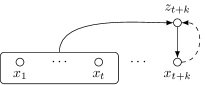
Figure 1: The proposed graphical model for generating acoustic frames. Solid lines denote the generative process, while the dashed line denotes the auxiliary distribution $q(z_{t+k}|x_{t+k})$.

Given the generative process, we propose to train the model with information-theoretic co-training [12] instead of the likelihood (1). Below we briefly review information-theoretic co-training under our setting.

The goal of co-training is to maximize the mutual information of the past $x_{1:t}$ and the discrete representation $z_{t+k}$ had we know the future frame $x_{t+k}$. We introduce an auxiliary distribution $q(z_{t+k}|x_{t+k})$ to simplify inference. By the definition of mutual information, we have that

$$I(z_{t+k},x_{1:t}|x_{t+k})=H(z_{t+k}|x_{t+k})-H(z_{t+k}|x_{1:t},x_{t+k}).$$ (3)

The key observation is that we can upper bound entropy with cross entropy and get

$$H(z_{t+k}|x_{1:t},x_{t+k}) =\mathbb{E}_{z_{t+k}\sim q}[-\log q(z_{t+k}|x_{1:t},x_{t+k})]$$

$$\leq\mathbb{E}_{z_{t+k}\sim q}[-\log p(z_{t+k}|x_{1:t},x_{t+k})],$$ (4)

where we have

$$p(z_{t+k}|x_{1:t},x_{t+k})\propto p(x_{t+k}|z_{t+k})p(z_{t+k}|x_{1:t})$$ (5)

using our independence assumptions in the graphical model. Combining (3) and (4), our final objective for the entire utterance, is thus

$$\mathcal{L} =\sum_{t=1}^{T-k}\mathbb{E}_{z_{t+k}\sim q}\big{[}-\log q(z_{t+k}|x_{t+k})$$

$$\qquad{}+\log p(x_{t+k}|z_{t+k})+\log p(z_{t+k}|x_{1:t})\big{]}.$$ (6)

The distributions are modeled with neural networks. In particular, $p(z_{z_{t+k}}|x_{1:t})$ is the prediction network, while $q(z_{t+k}|x_{t+k})$ is the confirmation network.

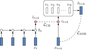
Figure 2: The forward process of training. The recurrent neural network and the quantization layer are trained jointly with the co-training objective.

For the prediction network, we choose a multilayer unidirectional recurrent network, allowing us to compare different training objectives, such as APC and VQ-APC, while holding the model architecture fixed. We apply a linear projection $U$ on the output of the recurrent network to obtain the probability of the latent variable. Formally,

$$p(z_{t+k}|x_{1:t})=p(z_{t+k}|h_{t})=\frac{\exp\left(h_{t}^{\top}U\mathbf{1}_{z_{t+k}}\right)}{\sum_{j=1}^{N}\exp\left(h_{t}^{\top}u_{j}\right)},$$ (7)

where $h_{t}$ is the output of the recurrent network after taking $x_{1:t}$ as input, $\mathbf{1}_{z_{t+k}}$ is a one-hot vector where the $z_{t+k}$-th element is set to 1, and $u_{j}$ is the $j$-th row of $U$.

For the confirmation network, we choose

$$q(z_{t+k}|x_{t+k})=\frac{\exp\left(-\|x_{t+k}-V\mathbf{1}_{z_{t+k}}\|^{2}\right)}{\sum_{j=1}^{N}\exp\left(-\|x_{t+k}-v_{j}\|^{2}\right)},$$ (8)

where $v_{j}$ is the $j$-th row of a matrix $V$. The distribution is chosen so that finding the mode of $q$ is equivalent to finding the closest row vector in $V$ to $x_{t+k}$. Given the similarity to VQ, we call $V$ the codebook, and each row vector in $V$ a codeword.

Finally, the generation distribution of the future frame is chosen as

$$p(x_{t+k}|z_{t+k})=\frac{1}{(2\pi)^{d/2}}\exp\left(-\frac{1}{2}\|x_{t+k}-WV\mathbf{1}_{z_{t+k}}\|^{2}\right),$$ (9)

where $W$ is a linear projection and $d$ is the dimension of $x_{t+k}$. In words, the probability can be interpreted as using the vector after quantization (one of the codewords) to generate $x_{t+k}$. For simplicity, we let each codeword have the same dimension as a frame and let $W$ be the identity matrix.

The parameters for training are the parameters in the recurrent network, $U$, $V$, and $W$ (if it weren’t fixed to the identity matrix). Note that based on the choice of distribution above, $\mathbb{E}_{z_{t+k}\sim q}[-\log p(z_{t+k}|x_{1:t})]$ is a cross-entropy (CE) loss, $\mathbb{E}_{z_{t+k}\sim q}[-\log p(x_{t+k}|z_{t+k})]$ is a weighted mean-squared-error (MSE) loss, and $\mathbb{E}_{z_{t+k}\sim q}[-\log q(z_{t+k}|x_{t+k})]$ is the entropy. The forward process is shown in Figure 2.

3 Related Work

Based on the loss functions and Figure 2, it is now clear that HuBERT-like training is a special case of our proposed approach. Specifically, the two steps

$$q(z_{t+k}|x_{t+k})=\mathbbm{1}[{z_{t+k}=\operatorname*{\arg\!\min\,}_{i=1,\dots,N}\|x_{t+k}-v_{i}\|}]$$ (10)

$$\min_{V}\sum_{t=1}^{T-k}\mathbb{E}_{z_{t+k}\sim q}[-\log p(x_{t+k}|z_{t+k})]$$ (11)

where $\mathbbm{1}[s]$ is 1 if $s$ is true and 0 otherwise, are exactly the steps in $k$-means. If we choose (10) instead of (8) as our confirmation network and optimize the codebook $V$ first before optimizing the recurrent network in (6), then our proposed approach is exactly HuBERT-like training, where $k$-means is first run offline and a model is trained to predict the $k$-means centroids [5]. This approach is only HuBERT-like, because (besides the architectural differences) there are subsequent clustering, pseudo-labeling, and training steps that are not covered in our approach. Another difference is that HuBERT uses an ad-hoc loss function when contrasting the quantized features, while our formulation simply uses cross entropy.

Several others [17, 18] have noted VQ as a hard E-step, i.e., the choise of $q$ in (10), in the context of variational expectation maximization, but the two training approaches have not been empirically compared.

Our approach subsumes VQ-APC if we optimize the likelihood (1) directly using Gumbel softmax to approximate the expectation (2). Specifically, we can write (2) as

$$p(x_{t+k}|x_{1:t})=\mathbb{E}_{z_{t+k}\sim p(z_{t+k}|x_{1:t})}[p(x_{t+k}|z_{t+k})].$$ (12)

The expectation can be approximated by drawing a single sample from the discrete distribution $p(z_{t+k}|x_{1:t})$. This can be achieved by adding Gumbel noise and a temperature to (7). The matrix $U$ is used to compute the sampling probability, while the matrix $V$ selects a codeword for the subsequent forward process. The matrix $W$ is also trained, and that completes the special case of VQ-APC.

Vector quantization has been widely applied to learning discrete units of speech [1, 19, 20] There is also evidence that enforcing discreteness in the model architecture learns a better representation for ASR [3, 6, 5, 7]. Each of these models is likely to have an underlying generative process similar to the one in Figure 1. Our work makes clear the connection between the generative process in Figure 1 and the forward process in Figure 2, explicitly showing where the discrete variables are assumed.

We also want to emphasize that while Gumbel softmax is often used as together with learning discrete representation, learning discrete representation does not neccessarily need to have Gumbel softmax. For example, since our generation distribution $p(x_{t+k}|z_{t+k})$ is shallow, exact marginalization is in fact efficient. Exact marginalization becomes expensive both in time and in memory when $p(x_{t+k}|z_{t+k})$ is deep, and that is when Gumbel softmax becomes neccessary, especially when using a large number of codewords.

4 Experiments

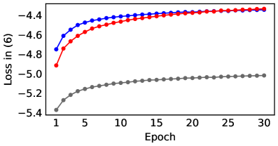
Figure 3: The co-training losses for various optimization approaches. The codebook size is $256$. At epoch $0$, the losses of exact marginalization, Gumbel approximation and HuBERT-like training are $-19.9$, $-19.9$ and $-8.4$ respectively. The epoch 0 losses are excluded for clarity.

One common belief is that the learned representation through self-supervision is highly correlated with phones [21, 2, 20]. To test this hypothesis, we pre-train our generative model on the 360-hour subset of LibriSpeech and perform phone classification on Wall Street Journal (WSJ). On top of this hypothesis, since our proposed approach subsumes HuBERT-like training and VQ-APC as special cases, we study the effect of different training approaches while holding the architecture fixed.

We extract 40-dimensional log Mel features for all data sets with a window size of 25 ms and a hop length of 10 ms. We normalize the acoustic frames based on the mean and variance of individual training sets. Following the protocol of prior work [13, 2, 22], we leave 10% of the training set si284 for development, and report phone error rates (PER) on the test set dev93. We use forced alignments obtained from a speaker-adaptive GMM-HMM as the ground truth.

We choose a 512-dimensional 3-layer unidirectional LSTM as the prediction network. We let the time shift $k=5$. For the confirmation network, we only use a codebook of size $N$, where each codeword is a 40-dimensional vector, the same dimension as the input frames. Regarding VQ-APC, we use a codebook of size $N$ with 512-dimensional codewords. For the targets of HuBERT-like training, we follow prior work [5] and use the $k$-means algorithm with $N$ centroids. We initialize the centroids with $k$-means++ [23] on randomly selected 3,000 utterances. Regular $k$-means is trained for 10 iterations. Once the models are pre-trained, we freeze the models and inspect the phonetic information in different layers of LSTMs by adding a linear projection on top of the hidden vectors.

A learning rate of $10^{-3}$ and a batch size of 16 are used for all experiments. We use Adam to optimize the pre-training objectives for 30 epochs, while only using 10 epochs for the linear classifier. Instead of using $\ell_{1}$ loss as in prior work [13, 2], our loss is MSE due to the choice of Gaussian. For Gumbel softmax, we cool the temperature $\tau$ from $2.0$ to $0.5$ with a decay rate of $0.99995$. Ths cooling schedule is used in both the sampling approximation of co-training and VQ-APC. We use the straight-through estimator when computing the gradient of the sampling.

4.1 Comparing Training Objectives

We train three variants based on the same objective in (6), HuBERT-like training, exact marginalization in (6), and a Gumbel approximation only for the term $\mathbb{E}_{z_{t+k}\sim q}[-\log p(z_{t+k}|x_{t+k})]$ to simulate the case when approximation is needed. In HuBERT-like training, only the cross entropy term $\mathbb{E}_{z_{t+k}\sim q}[-\log p(z_{t+k}|x_{1:t})]$ is optimized, since the other two terms are already optimized with $k$-means. We simply clamp $V$ to the $k$-means centroids when plotting the HuBERT-like objective. Despite using Gumbel approximation, we still report the exact marginalization of the loss. The training losses of the three variants are shown in Figure 3. Since $k$-means is trained off-line for HuBERT-like, its loss starts much higher than the other two. However, since the other two optimizes the entire objective, their losses rapidly surpass the HuBERT-like. We also find that using Gumbel approximation converges faster, but exact marginalization eventually becomes better.

Table 1: Phone error rates (PER) on dev93 for different learned representations. $N$ is the size of the codebook, and $h_{1}$, $h_{2}$, and $h_{3}$ indicate the use of the first, second, and third layer, respectively, for evaluation.

	$N$	PER(%) $\downarrow$
		$h_{1}$	$h_{2}$	$h_{3}$
APC	-	30.9	22.1	24.5
VQ-APC	100	28.1	22.4	30.0
	256	27.4	22.0	31.4
	512	27.2	22.4	31.2
HuBERT-like APC	100	24.9	20.5	26.2
	256	23.9	20.6	27.1
	512	22.6	21.1	27.9
Co-training (Gumbel)	100	24.7	19.9	25.1
	256	24.3	19.8	25.2
	512	24.9	19.8	25.1
Co-training (Marginalization)	100	26.0	19.7	24.4
	256	27.5	19.5	24.2
	512	26.3	19.5	24.8

4.2 Phone Classification Results

Given the three variants, we evaluate the learned representation with phone classification. We also compare vanilla APC and VQ-APC given how similar the approaches are. We use the same 3-layer unidirectional LSTM for all approaches. We experiment three codebook sizes, namely, 100, 256, and 512. The phone error rates (PER) are shown in Table 1.

We first notice that our reimplementation of APC is better than the prior work [13] due to various differences in the training pipeline. We observe better performance in the second layer, consistent with the general observation that phonetic information is more accessible in middle layers [13, 5]. HuBERT-like training is better than APC and VQ-APC, while both the Gumbel approximation and the exact marginalization are better than HuBERT-like. Optimizing the co-training objective with exact marginalization achieves an 11.8% relative improvement over vanilla APC, and a 4.9% relative improvement over HuBERT-like training.

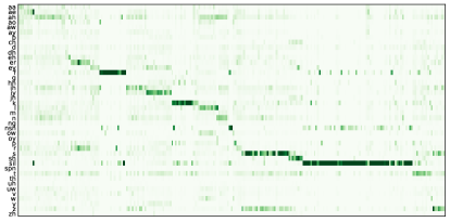
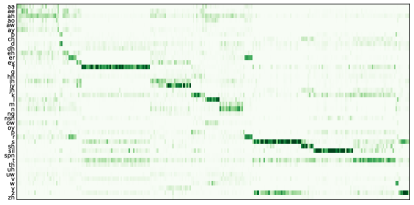
Figure 4: The conditional probabilities of phones given the codes evaluated on WSJ training set. The codes are based on the mode of either the prediction network (top) or confirmation network (bottom). The normalized mutual information is 0.228 (top) and 0.282 (bottom). The y-axis and x-axis represent the 42 phones and the codes respectively; the codebook size is $256$.

4.3 Correlation between phones and codes

Given the strong performance of phone classification, we expect the discrete representation (the codes in the codebook) to correlate well with phones. In Figure 4, we plot the conditional probabilities of phones given the codes (for $N=256$) based on co-occurrences on the WSJ training set. The codes are inferred based on either the mode of the prediction network (7) or the mode of the confirmation network (8). We observe a strong correlation between phones and codes for both. The codes correlate especially well with unvoiced fricatives, namely /f, s, sh/, and silences. The codes are also shared reasonably across phone classes, for example, between /s/ and /z/ for similar cutoff frequency, /r/ and /er/ for the distinct low F3, and /iy/ and /ey/ for sharing the high F2.

5 Conclusions

We have shown the strong performance of autoregressive co-training on learning discrete speech representation. Despite the simplicity of HuBERT-like training, predicting quantized acoustic frames alone gives a significant gain over APC. Optimizing the co-training objective gives the most significant gain. Our approach subsumes HuBERT-like training and VQ-APC, yet its generality has not been fully explored. Viable directions for future work include using a deep confirmation network and extending to discrete structures, similar to [24, 25].

References

- [1] J. Chorowski, R. J. Weiss, S. Bengio, and A. van den Oord, “Unsupervised speech representation learning using wavenet autoencoders,” IEEE Transactions on Audio, Speech, and Language Processing, 2019.
- [2] Y. Chung, H. Tang, and J. R. Glass, “Vector-quantized autoregressive predictive coding,” in Interspeech, 2020.
- [3] A. Baevski, Y. Zhou, A. Mohamed, and M. Auli, “wav2vec 2.0: A framework for self-supervised learning of speech representations,” 2020.
- [4] H. Zhou, A. Baevski, and M. Auli, “A comparison of discrete latent variable models for speech representation learning,” in ICASSP, 2021.
- [5] W. Hsu, B. Bolte, Y. H. Tsai, K. Lakhotia, R. Salakhutdinov, and A. Mohamed, “HuBERT: Self-supervised speech representation learning by masked prediction of hidden units,” IEEE Transactions on Audio, Speech, and Language Processing, 2021.
- [6] S. Ling and Y. Liu, “DeCoAR 2.0: Deep contextualized acoustic representations with vector quantization,” 2021.
- [7] Y. Chung, Y. Zhang, W. Han, C. Chiu, J. Qin, R. Pang, and Y. Wu, “w2v-BERT: Combining contrastive learning and masked language modeling for self-supervised speech pre-training,” in ASRU, 2021.
- [8] A. Mnih and K. Gregor, “Neural variational inference and learning in belief networks,” in ICML, 2014.
- [9] A. van den Oord, O. Vinyals, and K. Kavukcuoglu, “Neural discrete representation learning,” in NeurIPS, 2017.
- [10] C. J. Maddison, A. Mnih, and Y. W. Teh, “The concrete distribution: A continuous relaxation of discrete random variables,” in ICLR, 2017.
- [11] E. Jang, S. Gu, and B. Poole, “Categorical reparameterization with Gumbel-softmax,” in ICLR, 2017.
- [12] D. McAllester, “Information theoretic co-training,” arXiv:1802.07572, 2018.
- [13] Y. Chung, W. Hsu, H. Tang, and J. R. Glass, “An unsupervised autoregressive model for speech representation learning,” in Interspeech, 2019.
- [14] A. L.Maas, P. Qi, Z. Xie, A. Y. Hannun, C. T. Lengerich, D. Jurafsky, and A. Y.Ng, “Building DNN acoustic models for large vocabulary speech recognition,” Computer Speech & Language, 2017.
- [15] Y.-A. Chung and J. Glass, “Generative pre-training for speech with autoregressive predictive coding,” in ICASSP, 2020.
- [16] D. P. Kingma and M. Welling, “Auto-encoding variational Bayes,” in ICLR, 2014.
- [17] S. Jin, S. Wiseman, K. Stratos, and K. Livescu, “Discrete latent variable representations for low-resource text classification,” in ACL, 2020.
- [18] G. E. Henter, X. Wang, and J. Yamagishi, “Deep encoder-decoder models for unsupervised learning of controllable speech synthesis,” arXiv:1807:11470, 2018.
- [19] D. Harwath, W.-N. Hsu, and J. Glass, “Learning hierarchical discrete linguistic units from visually-grounded speech,” in ICLR, 2019.
- [20] B. van Niekerk, L. Nortje, and H. Kamper, “Vector-quantized neural networks for acoustic unit discovery in the ZeroSpeech 2020 Challenge,” in Interspeech, 2020.
- [21] A. Baevski, S. Schneider, and M. Auli, “vq-wav2vec: Self-supervised learning of discrete speech representations,” in ICLR, 2020.
- [22] A. H. Liu, Y. Chung, and J. R. Glass, “Non-autoregressive predictive coding for learning speech representations from local dependencies,” in Interspeech, 2021.
- [23] D. Arthur and S. Vassilvitskii, “k-means++: the advantages of careful seeding,” in SODA, 2007.
- [24] S. Bhati, J. Villalba, P. Zelasko, L. Moro-Velázquez, and N. Dehak, “Segmental contrastive predictive coding for unsupervised word segmentation,” in Interspeech, 2021.
- [25] J. Chorowski, G. Ciesielski, J. Dzikowski, A. Lancucki, R. Marxer, M. Opala, P. Pusz, P. Rychlikowski, and M. Stypulkowski, “Aligned contrastive predictive coding,” in Interspeech, 2021.