Quantum Annealing and Computation

Abstract

We introduce and review briefly the phenomenon of quantum annealing and analog computation. The role of quantum fluctuation (tunneling) in random systems with rugged (free) energy landscapes having macroscopic barriers are discussed to demonstrate the quantum advantage in the search for the ground state(s) through annealing. Quantum annealing as a physical (analog) process to search for the optimal solutions of computationally hard problems are also discussed.

Keywords: Adiabaticity, Analog computation, Cost function, D-wave annealer, Energy landscape, Ergodic, Escape probability, Entanglement, Fidelity, Free energy, Logic gates, Monte Carlo technique, Non-ergodic, Optical lattice, Photion cavity, Sherrington-Kirkpatrick model, Simulated annealing, Quantum annealing, Quantum tunneling, Spin glass, Time-dependent Schrodinger Equation, Travelling salesman problem

I Introduction

The idea of computation by decomposing the entire operation into elementary operations like addition, subtraction, etc, and eventually recasting the problem into just number crunching arithmetic, has been quite successful and popular. This has been possible because of the feasibility of binary digitization of the real numbers and availability of ever faster electronic logic gates (AND, OR, XOR, NOT, etc.).

The development and success of digital computers eclipsed the development of the analog computers, based on the dynamics of physical systems. Imagine a bowl on the table and you need to ‘locate’ its bottom point. Of course, one can calculate the local depths (from a reference height) everywhere along the inner surface of the bowl and search for the point where the local depth is maximum. However, as every one would easily guess, a much simpler and practical method could be to allow rolling of a marble ball along the inner surface of the bowl and wait for its resting location or position. Here, the physics of the forces of gravity and friction allows us to ‘calculate’ the location of the bottom-most (or minimum energy) point in an analog way! In principle, a similar trick would work for cases where the internal surface of the bowl has modulations, keeping the surface contour or the landscape valleys all tilted towards the same bottom point location. Problem comes when these valleys get separated by ‘barriers’, high enough.

Computationally hard problems, e.g., search of the ground state(s) of $N$-spin Sherrington-Kirkpatrick (SK) spin glass system sudip-sk involves locating the minima in a rugged landscape of size $2^{N}$, or exponential in $N$. The (free) energy landscape becomes rugged with occasional barriers of $N$ order, meaning that by flipping a countable few spins one can not get out of the local minimum. For that, one needs to flip a macroscopic number (of order $N$) to get out of the local minima. The same is true for the $N$-city Traveling Salesman Problem (see e.g., sudip-SA ) where one has to find the minimum cost (or travel distance) tours for visiting all the cities, from among the $N!$ order possible tours. Here also, perturbing a tour of higher travel length (cost function), by rearranging the local visit sequence (of a few cities), will not lead to success and one has to take a global view of modifying the sequence of visits to a finite fraction of the cities (effectively by overcoming $N$ order cost function barriers). Generally, for such minimum cost search from among $\exp(N)$ or higher configurations (or tours), often separated by $N$-order (energy or cost function) barriers, the search time can not be bounded by any polynomial in $N$ (NP-hard problems).

II Simulated (classical) annealing

In the seminal paper sudip-SA by Kirkpatrick et al., a novel stochastic technique was proposed based on the metallurgical annealing technique: To search for the optimized cost (energy of the ground state ‘crystal’) at eventually vanishing noise (or temperature $T$), one starts from a high noise ($T$) ‘melt’ phase, and tune slowly the noise level. In this ‘simulated noise’ tuning process, the (classical) noise at any intermediate level of annealing allows for the acceptance with (Gibbs-like) probability determined by the change in cost or energy (scaled by the noise factor) of even higher cost (energy) fluctuations. As the noise level ($T$) is slowly reduced during the annealing, the gradually decreasing probability of accepting higher cost values allows the system to come out of the local minima valleys and to settle eventually in the ‘ground state’ of the system with lowest cost (energy) value. It has been a remarkably successful trick for ‘practical’ computational solutions of a large class of multi-variable optimization problems in reasonable convergence time. For NP-hard problems, however, the search or convergence time for reaching the lowest cost state or configuration grows exponentially with $N$.

The bottleneck could be identified soon. Extensive study of the dynamics of frustrated random systems like the SK model showed that its (free) energy landscape (in the spin glass phase) is extremely rugged and the barriers, separating the local valleys, often become $N$ order for a $N$-spin glass. Same is true for $N$-city Traveling Salesman Problem. In the macroscopic size limit ($N$ approaching infinity) therefore such systems become (effectively) non-ergodic or localized and the classical (thermal) fluctuations, like that in the simulated annealing, fail to help the system to come out of such high barriers (at random locations or configurations, not dictated by any symmetry) as the escape probability is of order $\exp(-N/T)$ only. Naturally the annealing time (inversely proportional to the escape probability), to get the ground state of the $N$-spin SK model, can not be bounded by any polynomial in $N$.

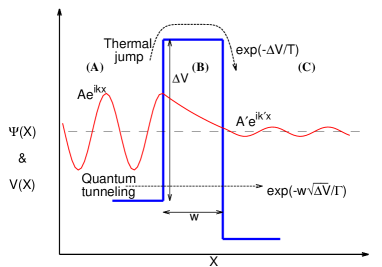
Figure 1: Schematic diagram suggesting the advantage of quantum tunneling over thermal hopping across a potential barrier. For kinetic energy ($E$) greater than the barrier potential $(V)$, compared to those in regions (A) and (C), the plane wave functions ($\psi(x)=A\exp(ikx)$ or $\psi(x)=A^{\prime}\exp(ik^{\prime}x)$) are indicated with (real) wave vectors $k=\sqrt{E-V}\simeq k^{\prime}$ in the two regions respectively. For region (B), the wave vector becomes imaginary (as $V>E$) and the consequent damping of the amplitude $A$ in region (A) to $A^{\prime}$ in region (C), occurs while passing through region (B). For $V$ of order $N$ and $E$ of order $N\Gamma$, the barrier transmission probability $(A^{\prime}/A)^{2}$ scales as $\exp(-w\sqrt{N(1-\Gamma)})\sim exp(-w\sqrt{N}/\Gamma)$.

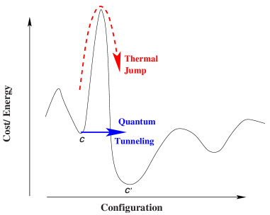
Figure 2: Optimizing the cost function of a computationally hard problem (for example, search for the ground state energy of a spin glass or for the minimum travel distance in a traveling salesman problem), one has to get out of a shallower local minimum (indicated here by the configuration $C$ of the spins in a spin glass or of a travel route of the salesman), to reach a deeper minimum (indicated here by $C^{\prime}$). This requires jumps or tunneling like fluctuations in the dynamics. Classically one has to jump over the energy or the cost barriers separating them, while (as indicated in Fig. 1) quantum mechanically one can tunnel through the same. With increasing barrier height, thermal jump becomes extremely difficult. However, if the barrier is narrow enough, quantum tunneling can help the search problem much easily.

III Quantum tunneling advantage for annealing

The indication sudip-ray was that quantum fluctuations in the SK model can perhaps lead to some escape routes to ergodicity or quantum fluctuation induced delocalization (at least in low temperature region of the spin glass phase) by allowing tunneling through such macroscopically tall but thin barriers which are difficult to scale using classical fluctuations. This is based on the argument that escape probability (see e.g., the discussion in ref. sudip-bikas ) due to quantum tunneling, from a single valley with single barrier of height $V$ and width $w$, scales as $\exp(-\sqrt{V}w/\Gamma)$; where $\Gamma$ represents the quantum fluctuation strength (or tunneling probability), while the classical (escape) probability is of order $\exp(-V/T)$ with $T$ denoting the temperature of the system (see Fig. 1). This extra handle through the barrier width $w$ (absent in the classical escape probability) helps in a major way in its vanishing limit. Indeed, for a single narrow ($w\rightarrow$ 0) barrier of height $N$, when the tunneling parameter $\Gamma$ is slowly tuned to zero, the annealing time to reach the ground state or optimized cost, will become $N$ independent! It has led to some important clues. Of course, complications (due to localization) may still arise for many such barriers at random locations.

In the Quantum Annealing scheme, the cost function of a multivariable optimization problem is mapped on to the energy function corresponding to a classical (frustrated) Hamiltonian ($H_{0}$). A time dependent quantum (non-commuting) kinetic term ($\Gamma(t)H^{\prime}$) is then added to the system. As $H^{\prime}$ does not commute with the $H_{0}$, it provides quantum dynamics to the overall system represented by the time dependent Hamiltonian $H(t)=H_{0}+\Gamma(t)H^{\prime}$ and the evolution of the system is given by the solution of the time dependent Schrödinger equation of the system

$$i{\hbar}{\frac{\partial\psi}{\partial t}}=\Big{[}\Gamma(t)H^{\prime}+H^{0}\Big{]}\psi.$$

If $\Gamma(0)$ is taken to be very large, then $\psi$ starts as the ground state of $H^{\prime}$, which is assumed to be known. As $\Gamma(t)$ starts decreasing slowly enough, following the quantum adiabatic theorem, the system will then be carried into the ground state of the instantaneous total Hamiltonian. At the end of the annealing schedule the kinetic term becomes zero ($\Gamma=0)$. Hence, one would expect the system to arrive at (one of) the ground state(s) of $H_{0}$, thereby giving the optimized value of the original cost function. We represent schematically the advantage of quantum annealing, compared to the classical one, using Fig. 2. This was first demonstrated sudip-Nishimori for random spin systems, by numerical solutions of the above Schrodinger equation for such systems. Indeed, the numerical results reported there for the annealing of a frustrated magnetic system (with less than ten spins), are shown in Fig. 3, indicating the clear advantage of tuning the quantum fluctuation, compared to the classical (thermal) one. The successive theoretical sudip-Farhi ; sudip-Santoro and experimental sudip-Brooke demonstrations led to the emergence of the field sudip-das .

Figure 3: Time dependence of the overlaps $P$ (with the ground state) of the frustrated model with $\Gamma(t)=T(t)=3/{\sqrt{t}}$ for classical and quantum annealing (subscripts ‘SA’ and ‘QA’ indicate simulated annealing and quantum annealing respectively, whereas superscript ‘st’ corresponds to quasistatic solution). [Fig. taken from ref. sudip-Nishimori ]

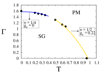
Figure 4: Phase diagram of quantum SK spin glass model as estimated from the Monte Carlo simulation and exact diagonalization. The spin glass and paramagnetic phases are denoted by SG and PM respectively. The data points at $T=0$ and $\Gamma=0$ are associated with the purely quantum and classical phase transitions, respectively. The two observed different critical behaviors of the system are indicated by blue (with the Binder cumulant $g_{c}$ near $0$ and the correlation length exponent value near $1/4$) and by yellow (with critical Binder cumulant $g_{c}$ near $0.22$ and correlation length exponent value near $1/2$) lines. The crossover in the critical behavior occurs around $T=0.49$ and $\Gamma=1.31$. [Fig. taken from ref. sudip-jsps ]

IV Quantum annealing in spin glasses

Using Suzuki-Trotter mapping of the quantum SK model to the effective classical spin model, Monte Carlo studies were conducted and annealing through ergodic and nonergodic regions of the model was studied sudip-jsps . Determination of thee phase diagram of the quantum SK model, employing the Monte Carlo simulation (at finite temperatures) and exact diagonalization technique (at zero temperature) revealed some interesting features. To extract the critical behavior at finite temperatures, different sizes (number of Ising spins ranging from $20$ to $180$) were considered in sudip-jsps , keeping constant the ratio of Trotter size and the effective dynamical size of the number of spins. At zero temperature, however, the maximum system size (for diagonalization study) had been of order 20 only. They found that from the quantum transition point ($T=0,\Gamma_{c}\simeq 1.63$) to almost the point ($T=0.45,\Gamma=1.33$), the critical Binder cumulant value remained vanishingly small (it can indeed effectively vanish even for non-Gaussian fluctuation-induced phase transitions). In this range of the phase boundary, they found the correlation length exponent to be about $1/4$ from the data collapse of Binder cumulant plots. In the rest of the phase boundary, the critical Binder cumulant value is about $0.22$ and they observed a satisfactory data collapse with the correlation length exponent equal to $1/2$. These two different values of the critical Binder comulant and the correlation length exponent for the two different parts of the phase boundary indicate the classical to quantum crossover (at $T\simeq 0.49$ and $\Gamma\simeq 1.31$; see Fig. 4) occurs at a non-vanishing value of temperature in the quantum SK model.

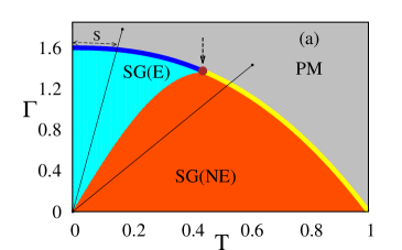
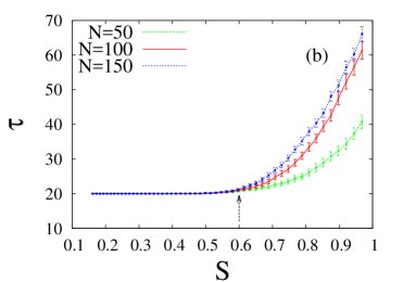
Figure 5: (a) Schematic phase diagram of the quantum SK model. The spin glass and paramagnetic phases are denoted by SG and PM, respectively. Numerical results showed sudip-jsps that the spin glass phase is further divided into two regions: ergodic spin glass phase SG(E) and nonergodic spin glass phase SG(NE). The quantum-classical crossover point in the critical behavior of the model is indicated by the red dot on the SG-PM phase boundary. The annealing behavior for the schedules $T(t)=T_{0}(1-t/\tau)$ and $\Gamma(t)=\Gamma_{0}(1-t/\tau)$, with $T_{0}$ and $\Gamma_{0}$ values corresponding to the paramagnetic phase are shown in (b). The Variation of annealing time $\tau$ with S, the length of the arc measured along the phase boundary (starting from the zero-temperature quantum transition point) to the intersection of the annealing line with the phase boundary. Low values of $S$ correspond to the SG(E)-PM phase boundary, while higher values of $S$ correspond to SG(NE)-PM boundary. The annealing time $\tau$ is clearly system size independent when the annealing path passes through the SG(E) region and increases rapidly with the system size when it pass through the SG(NE) region. [Fig. taken from ref. sudip-jsps ]

Unlike in the pure system (also in non-frustrated random system), where the free-energy landscape is smoothly inclined towards the global minima (Landau scenario), in the SK spin glass the landscape is extremely rugged. In particular, the local minima are often separated by system size dependent energy barriers which induce nonergodicity and the consequent replica-symmetry-broken distribution of the order parameter. Therefore, at any finite temperature the thermal fluctuations are unable to help the localized system to come out or escape from the macroscopically high free-energy barriers to reach the ground state (by flipping finite fraction of spins). With the aid of the transverse field the system can tunnel through such free-energy barriers sudip-ray ; sudip-bikas ; sudip-das . As a consequence, at low temperatures, the phase transition is governed by the quantum fluctuation and the system essentially exhibits quantum critical behavior (see the discussion on “possible restoration of ergodicity through quantum tunneling” for appropriate parameter space in the quantum SK model sudip-Leschke ).

Study on the nature of the order parameter distribution in the spin glass phase at finite temperatures through Monte Carlo simulations also showed sudip-jsps that in the high-temperature (low-transverse-field) classical fluctuation dominated spin glass region, along with the peak at the most probable value of the order parameter, the distribution contains a long tail (extending up to the zero value of the order parameter). This tail did not vanish even in the large system size limit, which indicated that the order parameter distribution remains Parisi type (replica Symmetry broken), corresponding to the nonergodic region SG(NE) (Fig. 5a) of the spin glass phase. On the other hand, in the low temperature (large transverse field) region, where the order parameter distribution effectively converges to a Gaussian form (with a peak around the most probable value) in the infinite-system-size limit. This indicates the existence of a single (replica-symmetric) order parameter in this ergodic region SG(E) of the spin glass phase. At zero temperature, the extrapolated order parameter distribution function showed a clear tendency to become one with a sharp peak (around the most probable value) in the large-system-size limit, suggesting the conclusion that the ergodic and non-ergodic regions of the spin glass phase are separated by a line possibly originating from point ($T=0,\Gamma=0$) and extending up to the quantum-classical crossover point ($T$ near $0.49$ and $\Gamma$ near $1.31$) on the phase boundary (see Fig. 5a). In order to find the role of such quantum-fluctuation-induced ergodicity in the (annealing) dynamics, they studied the variation of the annealing time $\tau$ (re- quired to reach close to the ground state(s)) with the system size following the schedules $T(t)=T_{0}(1-t/\tau)$ and $\Gamma(t)=\Gamma_{0}(1-t/\tau$). Attempts were made to reach a desired preassigned very low energy state (near the ground state) at the end of the annealing dynamics (in time $\tau$), keeping both $T$ and $\Gamma$ nonzero (but very small) at the end of the annealing schedule as the Suzuki-Trotter Hamiltonian (which governed the annealing dynamics) has singularities at both $T=0$ and $\Gamma=0$ (starting with $T_{0}$ and $\Gamma_{0}$ corresponding to the paramagnetic region of the phase diagram). They found (see Fig. 5b) that the average annealing time does not depend on the system size when annealing is carried out along paths that pass entirely through the ergodic region, whereas the annealing time becomes much larger and strongly size-dependent for paths that pass through the nonergodic region of the spin glass phase. These confirm the earlier observations sudip-ray ; sudip-bikas regarding the annealing time behavior, occurring due to tunneling through macroscopically tall but thin free-energy barriers in the SK model. In fact, the temporal variations of the average spin autocorrelation at finite temperatures also showed distinct behavior in these two regions of the spin glass phase of the quantum SK model. While at high temperatures, in the classical fluctuation dominated (nonergodic) region of the spin glass phase (SG(NE) region in Fig. 5a), one obtains very large values of the fitting relaxation times, the fitting relaxation times become order of magnitude smaller in the low temperature quantum fluctuation dominated region (SG(E) in Fig. 5a) presumably because of quantum tunneling sudip-jsps . These investigations clearly indicated the existence of a high-temperature (low-transverse-field) nonergodic region as well as a low-temperature (high-transverse-field) ergodic region in the spin glass phase. The line separating these two regions starts from $T=0$, $\Gamma=0$ and intersects the spin glass phase boundary at the quantum-classical crossover point (see Fig. 5(a)). The annealing behaviors are indicated in Fig. 5(b), showing that the annealing time $\tau$ is practically independent of $N$ when the annealing schedule (line) passes through the ergodic spin glass region (at low $T$ and high $\Gamma$).

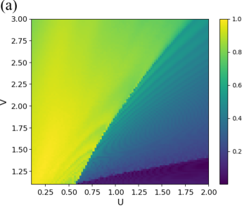
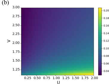
Figure 6: (a) Color density plot showing the solution fidelity after an adiabatic sweep using a Hamiltonian description with a classical mean-field approximation of the photon cavity modes. The parameter $U$ describes the particle-particle on-site repulsive interaction and the parameter $V$ represents the total potential depth of the specifically shifted lattice site, to create an impurity with a unique optimal solution. Three regions are clearly visible, a green-yellowish one, where the correct solution of two-particle on the mentioned lattice site is found, a bluish region with finite overlap but non-optimal solution, and a dark purple region with minimal overlap to the optimal solution. (b) Color density plot for the same parameter range showing the maximum entropy generated during the adiabatic sweep. In comparison, a connection between low maximum entropy and high success probability can be seen [Courtesy, E. Starchl sudip-Stachel ; private communication]

V Quantum annealer using optical lattice in a cavity

Indeed, Starchl and Ritsch sudip-Stachel studied a minimal Bose-Hubbard type system containing two atoms inside a cavity-generated optical lattice induced by an external trapping potential and directly pumped by two laser beams resulting in photon scattering into two separate cavity modes. Introduction of an additional local energy shift for a specific lattice site allows creating a unique energy separated optimal ground state for the problem Hamiltonian. The main focus was to compare the full quantum mechanical model with the semi-classical model, where the field mode induced interactions are approximated by classical coherent fields. The investigation revealed strong differences between the quantum and semi-classical model, which can be cast into a sort of phase diagram separating a distinct parameter region where (partial) quantum annealing does not find the optimum in the semi-classical approach, while full quantum annealing does. They found strong evidence for the involvement of entanglement in two ways. First, they sudip-Stachel confirmed the importance of vanishing entanglement at the end of the protocol and its influence on the minimal time needed for a successful simulation. Second, they identified a novel role of the maximum entanglement generated during the quantum annealing protocol in finding an optimal solution to the problem. They also studied the impact of different photon number cut-offs in the numerical quantum simulation. Most surprisingly they found improvement in the optimization success rate even for short simulation times when they used too low cut-off numbers to get a numerically accurate solution of the Schrödinger equation. Using higher cut-off numbers and thus a better representation of the exact quantum dynamics seems to be more relevant only for longer simulation times with very high success rates (see Fig. 6). These observations indicate a clear quantitative improvement of the annealing process for a full quantum system compared to a semi-classical one.

VI Outlook and further reading

Quantum Annealing is now a very well developed subject, both theoretically as well as experimentally (see e.g., sudip-das ; sudip-Brooke ). The breakthrough implementation of quantum annealing, employing superconducting qubits in successive generations of the D-wave annealers sudip-Johnson since 2011 and their availability in the market, has helped the growth of analog quantum computing in a major way. In fact, the availability of commercial quantum annealing condensed matter devices (like the D-wave systems) have revolutionized quantum information processing and computing algorithms for optimization across many disciplines, and led to developments which were unthinkable about a decade back. We would refer the readers to a few recent studies to get further informations and ideas. For discussions on quantum versus classical annealing the readers may consult ref. sudip-Heim , while for discussions on the efficiency of quantum versus classical annealing in the context of learning problems, the readers may consult ref. sudip-Baldassia (see sudip-Nath for a recent review on machine learning using quantum annealing). For a discussion on fault-tolerant quantum heuristics in the context of combinatorial optimizations, one may consult ref. sudip-Sanders , and ref. sudip-Pelofske for the indication of a major success using parallel quantum annealing algorithms. For a discussion on computer aided design of heterogeneous materials using quantum annealing algorithms, one may consult sudip-Sahimi . For recent extensive discussions on both theoretical and experimental developments, the readers are referred to the books sudip-Tanaka ; sudip-Dutta and reviews sudip-Albash ; sudip-Hauke .

Acknowledgement: We are thankful to our colleagues Arunava Chakrabarti, Arnab Das and Purusattam Ray for their contributions at various stages of this development over last three decades, to Gabriel Aeppli, Amit Dutta, Uma Divakaran, Jun-ichi Inoue, Atanu Rajak, Thomas Rosenbaum, Diptiman Sen, Parongama Sen, Sei Suzuki, Ryo Tamura and Shu Tanaka for collaborations on this and closely related topics over the years, and to Elias Starchl for his comments on the manuscript and help with Fig. 6. BKC is grateful to the Indian Academy of Sciences for their support through a Senior Scientist Research Grant. SM thanks the SERB, DST (India) for partial financial support through the TARE scheme [file no.:TAR/2021/000170] (2022).

References

- (1) D. Sherrington and S. Kirkpatrick, Phys. Rev. Lett. 35, 1792 (1975).
- (2) S. Kirkpatrick, C. D. Gelatt, and M. P. Vecchi, Optimization by Simulated Annealing, Science, 220, 671 (1983).
- (3) P. Ray, B. K. Chakrabarti and A. Chakrabarti, Phys. Rev. B. 39, 11828 (1989).
- (4) S. Mukherjee, B. K. Chakrabarti, Eur. Phys. J. Special Topics 224, 17 (2015).
- (5) T. Kadowaki and H. Nishimori, Phys. Rev. E, 58, 5355 (1998).
- (6) E. Farhi, J. Goldstone, S. Gutmann, J. Lapan, A. Ludgren and D. Preda, Science, 292, 472 (2001).
- (7) G. E. Santoro, R. Martoňák, E. Tosatti and R. Car, Science, 295, 2427 (2002).
- (8) J. Brooke, D. Bitko, T. F. Rosenbaum and G. Aeppli, Science 284, 779 (1999).
- (9) A. Das and B. K. Chakrabarti, Rev. Mod. Phys. 80, 1061 (2008).
- (10) S. Mukherjee and B. K. Chakrabarti, J. Phys. Soc. Jap., 88, 061004 (2019).
- (11) H. Leschke, C. Manai, R. Ruder and S. Warzel, Phys. Rev. Lett., 127, 207204 (2021).
- (12) E. Starchl and H. Ritsch, J. Phys. B: At. Mol. Opt. Phys. 55 (2022) 025501 (2022).
- (13) M. W. Johnson, M. H. S. Amin, S. Gildert, T. Lanting, F. Hamze, N. Dickson, R. Harris, A. J. Berkley, J. Johansson and P. Bunyk, Nature, 473, 194 (2011).
- (14) B. Heim, T. F. Rønnow, S. V. Isakov and M. Troyer, Science, 348, 215 (2015).
- (15) C. Baldassia and R. Zecchinaa, Proc. Nat. Acad. Sc., 115, 1457 (2018).
- (16) R. K. Nath, H. Thapliyal T. S. Humble, SN Comp. Sc., 2, 365 (2021).
- (17) Y. R. Sanders, D. W. Berry, P. C. S. Costa, L. W. Tessler, N. Wiebe, C. Gidney, H. Neven, and R. Babbush, PRX Quantum 1, 020312 (2020).
- (18) E. Pelofske, G. Hahn, H. N. Djidjev, Sci. Rep. 12, 4499 (2022).
- (19) M. Sahimi and P. Tahmasebi, Phys. Rep. 939, 1 (2021).
- (20) A. Dutta, G. Aeppli, B. K. Chakrabarti, U. Divakaran, T. F. Rosenbaum and D. Sen, Quantum Phase Transitions in Transverse Field Spin Models: From Statistical Physics to Quantum Information, Cambridge University Press, Cambridge (2015).
- (21) S. Tanaka, R. Tamura and B. K Chakrabarti, Quantum spin glasses, annealing and computation, Cambridge University Press, Cambridge (2017).
- (22) T. Albash and D. A. Lidar, Rev. Mod. Phys. 90, 015002 (2018).
- (23) P. Hauke, H. G. Katzgraber, W. Lechner, H. Nishimori and W. D. Oliver, Rep. Prog. Phys., 83, 054401 (2020).