Improved tetrahedron method for the Brillouin-zone integration applicable to response functions

Abstract

We improve the linear tetrahedron method to overcome systematic errors due to overestimations (underestimations) in integrals for convex (concave) functions, respectively. Our method is applicable to various types of calculations such as the total energy, the charge (spin) density, response functions, and the phonon frequency, in contrast with the Blöchl correction, which is applicable to only the first two. We demonstrate the ability of our method by calculating phonons in MgB₂ and fcc lithium.

I Introduction

In calculations of periodic systems on the basis of density functional theory (DFT)Hohenberg and Kohn (1964), integrals of matrix elements over the Brillouin zone (BZ) are evaluated to obtain various physical quantities of solids including the total energy, the electron (spin) density, the density of states, response functions, and the phonon frequency. Since this integral with respect to the Bloch wave vector $\bm{k}$ is replaced with a summation over a range of points described by a discrete variable $\bm{k}$, approximation schemes employed for this summation can significantly affect the accuracy and computational costs. Accurate integration using a modest number of $\bm{k}$ points is even more important for hybrid-DFT Perdew et al. (1996) and $GW$ approximation Hedin (1965), because in these cases the computational cost is proportional to the square of the number of $\bm{k}$ points, whereas standard semi-local approximations have a linear dependence.

There are two kinds of schemes to perform such an integration over the $\bm{k}$ points, namely, the broadening methodMethfessel and Paxton (1989) and the tetrahedron methodJepsen and Andersen (1971). In the broadening method, we replace the delta function with a smeared function which has a finite broadening width; we have to check the convergences about both the broadening width and the number of $\bm{k}$ points to obtain accurate results. In the tetrahedron method, we perform analytical integration in tetrahedral regions covering the BZ with the piecewise linear interpolation of a matrix element. Unlike the broadening method, we have to check the convergence only about the number of $\bm{k}$ points. The tetrahedron method is applied to calculations of susceptibility Rath and Freeman (1975), phonon frequency Savrasov (1992), phonon line width Savrasov and Savrasov (1996), and the local Green’s function as part of the dynamical mean field theory in the Hubbard model Fujiwara et al. (2003).

However, the tetrahedron method has a drawback; if a matrix element $A_{\bm{k}}$ is a convex (concave) function of $\bm{k}$, this method systematically overestimates (underestimates) its contribution to the integral due to the linear interpolation involved. Although this can be avoided by using the quadratic interpolation, we cannot perform analytical integration straightforwardly in such a case. The Blöchl correction Blöchl et al. (1994) was invented to overcome this issue by utilizing the following two facts: (i) the difference between the linear interpolation integration and that using the quadratic interpolation is approximately proportional to the second derivative of $A_{\bm{k}}$ integrated over the occupied region; (ii) although $\partial^{2}A_{\bm{k}}/\partial k^{2}$ cannot be evaluated within the framework of linear interpolation, we can perform the volume integral by replacing it with the Fermi surface integration of the first derivative of $A_{\bm{k}}$ (which can be evaluated by linear interpolation) using the Gauß theorem. Using this method we can reduce the number of $\bm{k}$ points to obtain converged results for total energies and charge densities. However, in the calculation of response functions or phonon frequencies, the integral $\int_{\epsilon_{\bm{k}}<\epsilon_{\rm F}}d^{3}kA_{\bm{k}}/(\epsilon_{\rm F}-\epsilon_{\bm{k}})$ appears, where $A_{\bm{k}}$ is an arbitrary function of $\bm{k}$. In this case, the Blöchl correction is inapplicable because we cannot perform the Fermi surface integration when $\partial(A_{\bm{k}}/(\epsilon_{\rm F}-\epsilon_{\bm{k}}))/\partial k$ is singular.

In this work, we develop a newly improved tetrahedron method that is applicable to calculations involving integrations of functions with singularities on the Fermi surfaces. It is constructed by means of a higher-order interpolation and the least square method. We apply our method to the BZ integration in calculations of phonon frequencies based on density functional perturbation theory (DFPT) Baroni et al. (2001). Following that we successfully calculate the frequency of phonons in MgB₂ and fcc Li. In contrast, it is difficult to achieve convergence in this calculation using conventional methods because the phonons in these materials couple strongly with electrons in the vicinity of Fermi surfaces Calandra et al. (2010); Bazhirov et al. (2010). In Sec. II, we describe our new tetrahedron method in detail after summarizing the conventional linear tetrahedron method and the Blöchl correction. Section III shows how our method improves the convergence about the number of $\bm{k}$ points in the calculation of phonons, followed by the conclusion in Sec. IV.

II Method

In this section, we introduce our new tetrahedron method; we begin with the standard linear tetrahedron method and the Blöchl correction to explain why these methods are not necessarily efficient in calculating response functions such as phonon frequencies.

II.1 The linear tetrahedron method and its drawbacks

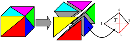
Figure 1: Sub-cell division into six tetrahedra and numbering of the tetrahedron corners; the red lines in the rightmost tetrahedron are the edges of the sub-cell.

We overview the general procedure of the tetrahedron method and its drawbacks. We calculate the integral

$$\int d^{3}kA_{\bm{k}}B(\epsilon_{\bm{k}}),$$ (1)

on the basis of the linear tetrahedron method, where $B(\epsilon_{\bm{k}})$ is a function of the orbital energy such as $\theta(\epsilon_{\rm F}-\epsilon_{\bm{k}})$, $\delta(\epsilon_{\rm F}-\epsilon_{\bm{k}})$, or $\theta(\epsilon_{\rm F}-\epsilon_{\bm{k}})/(\epsilon_{\rm F}-\epsilon_{\bm{k}})$. Here, $\theta(x)$ is the Heaviside step function. First, we divide a sub-cell into six tetrahedra (Fig. 1); this sub-cell is partitioned with the uniform $\bm{k}$-point mesh; for convenience, we number the corners of each tetrahedron from 1 to 4 along specific edges of the sub-cell (see Fig. 1). The contribution of this tetrahedron ($T$) to the integral (1) is

$$6V_{T}\int_{0}^{1}dx\int_{0}^{1-x}dy\int_{0}^{1-x-y}dzA_{T}({\bm{s}})B[\epsilon_{T}({\bm{s}})],$$ (2)

where ${\bm{s}}=(x,y,z)$, and

$$A_{T}({\bm{s}})\equiv A_{\bm{k}_{1}^{T}(1-x-y-z)+\bm{k}_{2}^{T}x+\bm{k}_{3}^{T}y+\bm{k}_{4}^{T}z},$$ (3)

$$\epsilon_{T}({\bm{s}})\equiv\epsilon_{\bm{k}_{1}^{T}(1-x-y-z)+\bm{k}_{2}^{T}x+\bm{k}_{3}^{T}y+\bm{k}_{4}^{T}z},$$ (4)

where $\bm{k}_{i}^{T}$ is the $\bm{k}$ point of the $i$th corner of $T$. In the linear tetrahedron method, we approximate $A_{T}$ and $\epsilon_{T}$ with linear functions:

$$A_{T}^{1}({\bm{s}}) =A_{1}(1-x-y-z)+A_{2}x+A_{3}y+A_{4}z,$$ (5)

$$\epsilon_{T}^{1}({\bm{s}}) =\epsilon_{1}(1-x-y-z)+\epsilon_{2}x+\epsilon_{3}y+\epsilon_{4}z,$$ (6)

where $A_{i}$ and $\epsilon_{i}$ are the matrix element and the orbital energy at the $i$th corner, respectively. The integration (2) with formulae (5) and (6) is performed analytically.

However, linear interpolation has a drawback; if the matrix element $A_{T}({\bm{s}})$ is a convex function within the tetrahedron $T$, the interpolated function $A_{T}^{1}({\bm{s}})$ becomes $A_{T}^{1}({\bm{s}})\geq A_{T}({\bm{s}})$ in $T$; hence, the integral is systematically overestimated. If $A_{T}({\bm{s}})$ is a concave function, the sign of the inequality is reversed (see Fig. 2(a)).

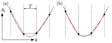
Figure 2: Two kinds of approximations of the matrix element. True and approximated matrix elements $A_{T}$ are depicted as black dash-doted lines and red solid lines, respectively; the black points indicate the matrix elements $A_{\bm{k}}$ for a given value of $\bm{k}$; the dashed lines indicate the boundaries of the tetrahedra. (a) The liner interpolated function $A_{T}^{1}$ is always smaller (larger) than the true function $A_{T}$ in the case of a convex (concave) function. (b) The leveled linear function is a better approximation of the true function.

II.2 The Blöchl correction and its limitation

In the special case that the integral (1) becomes

$$\int d^{3}kA_{\bm{k}}\theta(\epsilon_{\rm F}-\epsilon_{\bm{k}}),$$ (7)

we can overcome the drawback of the linear tetrahedron method by considering the curvature of $A_{\bm{k}}$ within the framework of the linear interpolation Blöchl et al. (1994); this type of integration appears in the calculations of total energies or charge (spin) densities. In this case, we can evaluate the difference between the integral (7) with the linear interpolation of $A_{\bm{k}}$ ($A^{\rm lin}$) and that with the quadratic interpolation ($A^{\rm quad}$) as follows. First, we write this difference as

$$\Delta A\equiv A^{\rm quad}-A^{\rm lin}=\sum_{T}^{\epsilon_{\bm{k}}\leq\epsilon_{\rm F}}\sum_{ij}C_{ij}^{T}\Braket{\frac{\partial^{2}A_{\bm{k}}}{\partial k_{i}\partial k_{j}}}_{T},$$ (8)

where $C_{ij}^{T}$ is the form factor describing the shape and the orientation of the tetrahedron as follows

$$C_{ij}^{T}=\frac{1}{40}\left[\sum_{l=1}^{4}(\bm{k}_{l}^{T})_{i}\sum_{m=1}^{4}(\bm{k}_{m}^{T})_{j}-4\sum_{l=1}^{4}(\bm{k}_{l}^{T})_{i}(\bm{k}_{l}^{T})_{j}.\right],$$ (9)

and $\Braket{\cdots}_{T}$ indicates an integration in the tetrahedron $T$. Now, we replace $\partial^{2}A_{\bm{k}}/\partial k^{2}$ with $\partial A_{\bm{k}}/\partial k$ because the former cannot be evaluated in the framework of the linear interpolation, but the latter can be. We assume the form factor is a constant over the entire BZ ($C_{ij}^{T}\approx C_{ij}$), and then we apply the Gauß theorem:

$$\Delta A \approx\sum_{ij}C_{ij}\int_{\epsilon_{\bm{k}}<\epsilon_{\rm F}}d^{3}k\frac{\partial^{2}A_{\bm{k}}}{\partial k_{i}\partial k_{j}}$$

$$=\sum_{ij}C_{ij}\int_{\epsilon_{\bm{k}}=\epsilon_{\rm F}}d^{2}k\frac{(\nabla_{\bm{k}}\epsilon_{\bm{k}})_{i}}{|\nabla_{\bm{k}}\epsilon_{\bm{k}}|}\frac{\partial A_{\bm{k}}}{\partial k_{j}}$$

$$\approx\sum_{T}^{{\rm Fermisurface}}\sum_{ij}C_{ij}^{T}\left\langle\frac{(\nabla_{\bm{k}}\epsilon_{\bm{k}})_{i}}{|\nabla_{\bm{k}}\epsilon_{\bm{k}}|}\frac{\partial A_{\bm{k}}}{\partial k_{j}}\right\rangle_{T}$$ (10)

However, when we calculate an integral such as

$$\int d^{3}kA_{\bm{k}}\frac{\theta(\epsilon_{\rm F}-\epsilon_{\bm{k}})}{\epsilon_{\rm F}-\epsilon_{\bm{k}}},$$ (11)

(this kind of integration appears in the calculations of response functions and phonon frequencies), the difference associated with the two kinds of interpolation becomes

$$\Delta A=\sum_{T}^{\epsilon_{\bm{k}}<\epsilon_{\rm F}}\sum_{ij}C_{ij}^{T}\Braket{\frac{\partial^{2}A_{\bm{k}}}{\partial k_{i}\partial k_{j}}}_{T}G(\epsilon_{\bm{k}},\nabla_{\bm{k}}\epsilon_{\bm{k}}),$$ (12)

where $G(\epsilon_{\bm{k}},\nabla_{\bm{k}}\epsilon_{\bm{k}})$ is a complicated function of $\epsilon_{\bm{k}}$ and $\nabla_{\bm{k}}\epsilon_{\bm{k}}$; therefore, we cannot apply the Blöchl correction because we cannot replace $\partial^{2}A_{\bm{k}}/\partial k^{2}$ with $\partial A_{\bm{k}}/\partial k$ as before. This is due to the presence of the energy denominator; hence, we have to start with another concept to overcome this issue.

II.3 A newly improved tetrahedron method applicable to response functions

The systematic error of the tetrahedron method is a result of the linear interpolation. Although we can avoid this problem if we use higher order interpolation, the integral (2) becomes unsolvable analytically. The real question is: how can we improve the linear approximation of the matrix elements? The answer is to employ leveling rather than interpolating (see fig. 2 b). The procedure is explained below.

1. We construct the $N$th polynomial $A_{T}^{N}({\bm{s}})$ from $A_{\bm{k}}$ and $\bm{k}$ using the corners of a tetrahedron $T$ and some additional surrounding points for sampling.

2. We fit a linear function

   $$A_{T}^{LSM}({\bm{s}})={\bar{A}}_{1}(1-x-y-z)+{\bar{A}}_{2}x+{\bar{A}}_{3}y+{\bar{A}}_{4}z$$ (13)

   into $A_{T}^{N}({\bm{s}})$ through the least square method (LSM); that is to say, we solve

   $$\frac{\partial}{\partial{\bar{A}}_{i}}\int_{0}^{1}dx \int_{0}^{1-x}dy\int_{0}^{1-x-y}dz$$

   $$\times|A_{T}^{N}({\bm{s}})-A_{T}^{LSM}({\bm{s}})|^{2}=0.$$ (14)

3. We apply the same procedure to $\epsilon_{\bm{k}}$, and obtain $\epsilon_{T}^{LSM}({\bm{s}})$.

4. We evaluate integral (2) replacing $A_{T}({\bm{s}})$ and $\epsilon_{T}({\bm{s}})$ with $A_{T}^{LSM}({\bm{s}})$ and $\epsilon_{T}^{LSM}({\bm{s}})$, respectively.

5. We repeat the above steps for all tetrahedra.

Although the approximated matrix element $A_{T}^{LSM}({\bm{s}})$ is discontinuous at boundaries of tetrahedra (see Fig. 2(b)), it is of no concern because we are interested only in the integrated value.

II.4 Implementation

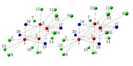
Figure 3: Points for constructing a third order interpolation function (parallel stereogram). Red points denote the corners of $T$. The blue and green points are explained in Table 1.

Table 1: Points for constructing a third order interpolation function

Nearest neighbor points on extended lines
of each edge of $T$ (green balls in Fig. 3).
$\bm{k}_{5}=2\bm{k}_{1}-\bm{k}_{2}$	$\bm{k}_{9}=2\bm{k}_{1}-\bm{k}_{3}$	$\bm{k}_{13}=2\bm{k}_{1}-\bm{k}_{4}$
$\bm{k}_{6}=2\bm{k}_{2}-\bm{k}_{3}$	$\bm{k}_{10}=2\bm{k}_{2}-\bm{k}_{4}$	$\bm{k}_{14}=2\bm{k}_{2}-\bm{k}_{1}$
$\bm{k}_{7}=2\bm{k}_{3}-\bm{k}_{4}$	$\bm{k}_{11}=2\bm{k}_{3}-\bm{k}_{1}$	$\bm{k}_{15}=2\bm{k}_{3}-\bm{k}_{2}$
$\bm{k}_{8}=2\bm{k}_{4}-\bm{k}_{1}$	$\bm{k}_{12}=2\bm{k}_{4}-\bm{k}_{2}$	$\bm{k}_{16}=2\bm{k}_{4}-\bm{k}_{3}$
Remaining corners of tetrahedra
that share surfaces with $T$ (blue balls in Fig. 3).
$\bm{k}_{17}=\bm{k}_{4}-\bm{k}_{1}+\bm{k}_{2}$           $\bm{k}_{18}=\bm{k}_{1}-\bm{k}_{2}+\bm{k}_{3}$
$\bm{k}_{19}=\bm{k}_{2}-\bm{k}_{3}+\bm{k}_{4}$           $\bm{k}_{20}=\bm{k}_{3}-\bm{k}_{4}+\bm{k}_{1}$

We use a third order polynomial $A_{T}^{3}({\bm{s}})$ as $A_{T}^{N}({\bm{s}})$ in our implementation. The sampling points used to construct $A_{T}^{3}({\bm{s}})$ are the corners of the tetrahedron $T$ (4 points) and the other 16 points given in Table 1 and Fig. 3. As a result, $A_{T}^{3}({\bm{s}})$ becomes

$$A_{T}^{3} ({\bm{s}})=\frac{A_{1}}{2}u(u+1)(2-u)+\frac{A_{2}}{2}x(x+1)(2-x)$$

$$+\frac{A_{3}}{2}y(y+1)(2-y)+\frac{A_{4}}{2}z(z+1)(2-z)$$

$$-\frac{u^{2}x}{6}(2A_{5}+A_{14})-\frac{x^{2}y}{6}(2A_{6}+A_{15})$$

$$-\frac{y^{2}z}{6}(2A_{7}+A_{16})-\frac{z^{2}u}{6}(2A_{8}+A_{13})$$

$$-\frac{u^{2}y}{6}(2A_{9}+A_{11})-\frac{x^{2}z}{6}(2A_{10}+A_{12})$$

$$-\frac{y^{2}u}{6}(2A_{11}+A_{9})-\frac{z^{2}x}{6}(2A_{12}+A_{10})$$

$$-\frac{u^{2}z}{6}(2A_{13}+A_{8})-\frac{x^{2}u}{6}(2A_{14}+A_{5})$$

$$-\frac{y^{2}x}{6}(2A_{15}+A_{6})-\frac{z^{2}y}{6}(2A_{16}+A_{7})$$

$$+(A_{2}+A_{4})xz(u+y)+(A_{1}+A_{3})uy(x+z)$$

$$-\left(A_{17}+\frac{A_{10}+A_{12}}{2}+\frac{A_{5}-A_{14}}{6}+\frac{A_{13}-A_{8}}{6}\right)xzu$$

$$-\left(A_{18}+\frac{A_{9}+A_{11}}{2}+\frac{A_{6}-A_{15}}{6}+\frac{A_{14}-A_{5}}{6}\right)xyu$$

$$-\left(A_{19}+\frac{A_{10}+A_{12}}{2}+\frac{A_{7}-A_{16}}{6}+\frac{A_{15}-A_{6}}{6}\right)xyz$$

$$-\left(A_{20}+\frac{A_{9}+A_{11}}{2}+\frac{A_{8}-A_{13}}{6}+\frac{A_{16}-A_{7}}{6}\right)yzu,$$ (15)

where $u=1-x-y-z$. By substituting it into (2), we obtain $A_{T}^{LSM}({\bm{s}})$:

$${\bar{A}}_{i}=\sum_{j=1}^{20}P_{ij}A_{\bm{k}_{j}},$$ (16)

where

$${\bf P}=({\bf P}^{(1)},{\bf P}^{(2)},{\bf P}^{(3)},{\bf P}^{(4)},{\bf P}^{(5)}),$$ (17)

$${\bf P}^{(1)} =\frac{1}{1260}\begin{pmatrix}1440&0&30&0\\ 0&1440&0&30\\ 30&0&1440&0\\ 0&30&0&1440\end{pmatrix},$$ (18)

$${\bf P}^{(2)} =\frac{1}{1260}\begin{pmatrix}-38&7&17&-28\\ -28&-38&7&17\\ 17&-28&-38&7\\ 7&17&-28&-38\end{pmatrix}={}^{t}{\bf P}^{(4)},$$ (19)

$${\bf P}^{(3)} =\frac{1}{1260}\begin{pmatrix}-56&9&-46&9\\ 9&-56&9&-46\\ -46&9&-56&9\\ 9&-46&9&-56\end{pmatrix},$$ (20)

$${\bf P}^{(5)} =\frac{1}{1260}\begin{pmatrix}-18&-18&12&-18\\ -18&-18&-18&12\\ 12&-18&-18&-18\\ -18&12&-18&-18\end{pmatrix}.$$ (21)

We go through the same procedure for the orbital energy $\epsilon_{\bm{k}}$.

We can consider this procedure in a different way; when we calculate the contribution from a tetrahedron, we use the linear tetrahedron method after we have replaced matrix elements and orbital energies with those given in (16). Using this idea, we represent the integration (1) as

$$\int d^{3}kA_{\bm{k}}B(\epsilon_{\bm{k}})=\sum_{\bm{k}}A_{\bm{k}}w_{\bm{k}},$$ (22)

where $w_{\bm{k}}$ is calculated as follows:

1. We divide the BZ into tetrahedra.

2. We calculate effective orbital energies as

   $${\bar{\epsilon}}_{i}=\sum_{j=1}^{20}P_{ij}\epsilon_{\bm{k}_{j}^{T}}$$ (23)

   for the corners of each tetrahedron.

3. We calculate the effective weight ${\bar{w}}^{T}_{i}$ using the standard linear tetrahedron method with the effective orbital energy (23).

4. $w_{\bm{k}}$ is calculated as

   $$w_{\bm{k}}=\sum_{T}\sum_{i=1}^{4}\sum_{j=1}^{20}P_{ij}{\bar{w}}^{T}_{i}\delta(\bm{k}-\bm{k}^{T}_{j}).$$ (24)

III Comparison with other integration schemes for actual calculations

We implement our method in an ab initio electronic structure calculation code Quantum ESPRESSOGiannozzi et al. (2009) which uses plane waves to represent Kohn-Sham (KS) orbitals. Then, we test the effectiveness of the method through calculations of phonons in two systems, MgB₂ Nagamatsu et al. (2001) and fcc lithium at a high pressure (20 GPa), based on DFPT Baroni et al. (2001)(Appendix A).

Magnesium diboride has the highest $T_{C}$ (about 40 K) out of the known phonon-type superconductors. Many ab initio studies have been performed since it was discovered Calandra et al. (2010); Kong et al. (2001); Bohnen et al. (2001); Choi et al. (2002); Eiguren and Ambrosch-Draxl (2008), revealing that the high $T_{C}$ is a result of the strong interaction between intra-layer vibrations of B atoms and their covalent bonding orbitals ($\sigma$ bands) (Fig. 4).

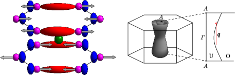
Figure 4: (left) The Mg centered Wigner-Seits cell of MgB₂. Green and purple spheres indicate Mg and B atoms respectively. The $\sigma$ orbital (blue and red isosurfaces of opposite signs.) and the displacement pattern of the intra-layer vibrational mode of the B atoms with wave number $\bm{q}$ at the $A$ point (arrows) are also depicted. (right) Schematic illustration of the Fermi surfaces of the $\sigma$ bands; the red arrow indicates the momentum vector of a phonon at the $A$ point which connects occupied (O) and unoccupied (U) regions in the vicinity of the Fermi surface.

This strong coupling also softens phonon frequencies due to the screening of the ion-ion interaction; this screening occurs due to linear responses of $\sigma$ electrons in the vicinity of the Fermi surfaces. We have to evaluate these responses accurately to determine the phonon frequencies precisely. Lithium exhibits a monatomic fcc structure at pressures between 7.5 and 39 GPa Hanfland et al. (2000). In this phase it becomes a superconductor. Its $T_{C}$ increases with pressure up to 30 GPa Deemyad and Schilling (2003); Struzhkin et al. (2002); Shimizu et al. (2002) because of the growth of the electron-phonon interaction. The lower transverse acoustic mode at $\bm{q}\approx\overrightarrow{\Gamma K}$ couples with electrons most strongly in this material Bazhirov et al. (2010). In this test, we consider the phonons of fcc Li at a pressure of 20 GPa.

We use norm-conserving pseudopotentials Hamann et al. (1979) in calculations of MgB₂; the cutoff energy of plane waves is set to 50 Ry. In the calculations of fcc lithium, we use an ultrasoft pseudopotentialVanderbilt (1990). We treat the electrons in the 1s orbitals as valence electronsPse and employ a cutoff energy of 80 Ry. In both of these applications, we use the GGA-PBE functional Perdew et al. (1997) and the first-order Hermite-Gaussian function de Gironcoli (1995); Methfessel and Paxton (1989) for broadening.

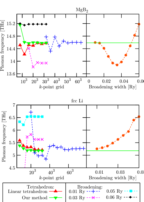
Figure 5: (left) The $\bm{k}$ convergences of the frequencies of the intra-layer vibrational mode of the B atoms at the $A$ point in the BZ for MgB₂ (top) and the lower transverse acoustic mode at the $K$ point in the BZ for fcc Li at 20 GPa (bottom) with a different $\bm{k}$ integration method. $\blacktriangle$ and $\blacktriangledown$ with red and green solid lines are the results of the linear and improved tetrahedron methods; $+$, $\times$, $\blacksquare$, and $\blacklozenge$ with blue, purple, cyan, and black dashed lines denote the results of the broadening method for widths of 0.01, 0.03, 0.05, and 0.06 Ry, respectively. Lines are guides for the eyes. (right) The frequency of these modes converged about the number of $\bm{k}$ at each broadening width ($\bullet$ with orange line); the green solid lines indicate the converged value obtained by our method.

We apply our method to the calculation of the frequency of the intra-layer vibrational mode of B atoms at the $A$ point in the BZ (Fig. 5 top left). The result of the improved tetrahedron method converges faster than that of the linear tetrahedron method; it converges with approximately $12^{3}$ $\bm{k}$ points. If we use a broadening method with a small broadening width (0.01 Ry), the result converges at an unrealistically large number of $\bm{k}$ points (about $50^{3}$ $\bm{k}$ points). On the other hand, using large broadening widths (0.03 Ry and 0.06 Ry), convergence occurs at a lower number of $\bm{k}$ points. However, results are far away from the one converged about the broadening width; The complicated dependence of the convergence on the broadening width is shown in the top-right panel of Fig. 5. The result cannot be represented by a simple function, so it is difficult to extrapolate to a broadening width of zero.

The bottom left panel of Fig. 5 shows the $\bm{k}$ convergence of the lower transverse acoustic mode at the $K$ point in the BZ for fcc Li at 20 GPa calculated with the different integration schemes. Our method achieves convergence very quickly; it requires only $16^{3}$ $\bm{k}$ points. In this system, the result of the broadening method is very sensitive to the broadening width; the error due to broadening is more than 25 % at a width of 0.05 Ry; hence, the broadening method is not suitable for this calculation.

We will show how the accuracy of the phonon calculations affects the prediction of the superconducting transition temperature within the framework of the following McMillan formula McMillan (1968); Dynes (1972):

$$T_{C}=\frac{\omega_{\log}}{1.2}\exp\left(\frac{-1.04(1+\lambda)}{\lambda-\mu^{*}(1+0.62\lambda)}\right),$$ (25)

Here,

$$\lambda=\sum_{\bm{q}\nu\bm{k}nn^{\prime}}\frac{2}{D(\epsilon_{\rm F})\omega_{\bm{q}\nu}}$$

$$\hskip 30.00005pt\times|g_{n\bm{k}n^{\prime}\bm{k}+\bm{q}}^{\bm{q}\nu}|^{2}\delta(\epsilon_{n\bm{k}}-\epsilon_{\rm F})\delta(\epsilon_{n^{\prime}\bm{k}+\bm{q}}-\epsilon_{\rm F})$$ (26)

and

$$\log(\omega_{\log})=\frac{1}{\lambda}\sum_{\bm{q}\nu\bm{k}nn^{\prime}}\frac{2}{D(\epsilon_{\rm F})\omega_{\bm{q}\nu}}\log(\omega_{\bm{q}\nu})$$

$$\hskip 30.00005pt\times|g_{n\bm{k}n^{\prime}\bm{k}+\bm{q}}^{\bm{q}\nu}|^{2}\delta(\epsilon_{n\bm{k}}-\epsilon_{\rm F})\delta(\epsilon_{n^{\prime}\bm{k}+\bm{q}}-\epsilon_{\rm F}),$$ (27)

where $\omega_{\bm{q}\nu}$ is the phonon frequency with the wave number $\bm{q}$ and the branch $\nu$, $\epsilon_{n\bm{k}}$ is the KS eigenvalue with the wave number $\bm{k}$ and the band index $n$, and $D(\epsilon_{\rm F})$ is the density of states per spin at the Fermi energy. The electron-phonon coupling constant $g_{n\bm{k}n^{\prime}\bm{k}+\bm{q}}^{\bm{q}\nu}$ is written in the form

$$g_{n\bm{k}n^{\prime}\bm{k}+\bm{q}}^{\bm{q}\nu}=\sum_{\tau\alpha}\frac{(\eta_{\bm{q}\nu})_{\tau\alpha}}{\sqrt{M_{\tau}\omega_{\bm{q}\nu}}}\Braket{n^{\prime},\bm{k}+\bm{q}}{\frac{\delta v_{S}}{\delta R_{\tau\alpha}(\bm{q})}}{n,\bm{k}},$$ (28)

where $M_{\tau}$ is a mass of an ion, $(\eta_{\bm{q}\nu})_{\tau\alpha}$ is the unit displacement pattern of the phonon $(\bm{q},\nu)$, $\Ket{n,\bm{k}}$ is the KS orbital, and ${\delta v_{S}}/{\delta R_{\tau\alpha}(\bm{q})}$ is the linear response of the KS potential with respect to the distortion of the wave number $\bm{q}$; $\tau$ and $\alpha$ are indices of an ion in the unit cell and a direction in the Cartesian coordinate, respectively. Although there are more precise methods to calculate $T_{C}$ such as density functional theory for superconductors Oliveira et al. (1988); Lüders et al. (2005), we use this simple formula because we are only interested in changes in the results due to the $\bm{k}$ integration in the phonon calculations.

To evaluate the integrals in (III) and (III) , we use the linear tetrahedron method with a $\bm{q}$ grid of $6\times 6\times 4$ ($8\times 8\times 8$) and a $\bm{k}$ grid of $24\times 24\times 18$ ($32\times 32\times 32$) for MgB₂ (fcc Li), respectively. Additionally, we calculate each $\omega_{\bm{q}\nu}$ and ${\delta v_{S}}/{\delta R_{\tau\alpha}(\bm{q})}$ with different $\bm{k}$ grids and different $\bm{k}$ integration schemes.

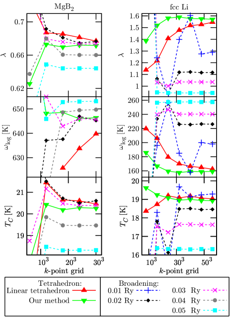
Figure 6: The $\bm{k}$ convergences of $\lambda$ (top), $\omega_{\log}$ (middle), and $T_{C}$ from the McMillan’s formula (bottom) of MgB₂ (left) and fcc Li (right) calculated using $\omega_{\bm{q}\nu}$ and ${\delta v_{S}}/{\delta R_{\tau\alpha}(\bm{q})}$ with different $\bm{k}$ integration schemes; $\blacktriangle$ and $\blacktriangledown$ with red and green solid lines are the results of the linear and improved tetrahedron methods; $\blacklozenge$, $+$, $\times$, $\blacksquare$, and $\bullet$ with gray, blue, purple, black, and cyan dashed lines denote the results of broadening methods of widths 0.01, 0.02, 0.03, 0.04, and 0.05 Ry respectively; Lines are guides for the eyes.

Figure 6 shows the result of $\lambda$, $\omega_{\log}$, and $T_{C}$ from the McMillan’s formula ($\mu^{*}=0.1$); in both the MgB₂ and Li cases, we obtain very fast $\bm{k}$ convergence using our method. Comparing the $\bm{k}$ converged result of our method to that of the broadening method with a width of 0.05 Ry, we can see a large overestimate of the phonon frequencies occurs when the broadening method is used, resulting in an underestimated $\lambda$ and an overestimated $\omega_{\log}$. Moreover, speeds of convergences about the broadening width for calculations of the $\lambda$ and $\omega_{\log}$ are very slow; these results have not reach the convergence even for the broadening width of 0.01 Ry; if we use smaller broadening width (such as 0.005 Ry), we need an unrealistic number of $\bm{k}$ points to obtain the $\bm{k}$-converged result.

IV Conclusion

We introduced an improvement to the tetrahedron method based on the third order interpolation and the least square method that reduces the number of $\bm{k}$ points required to obtain converged results of the BZ integrations. Our method is applicable to various kinds of $\bm{k}$-integration; in particular, it is efficient for calculations of phonons and response functions because the associated computational costs are large and the Blöchl correction is not applicable to these calculations. We demonstrated this effectiveness through calculations of phonon frequencies in MgB₂ and fcc Li.

Appendix A Calculation of weights for DFPT

The integration weights for the DFPT calculations of phonon frequencies are different from those of the total energy, $\theta(\epsilon_{\rm F}-\epsilon_{nk})$, or the density of states, $\delta(\epsilon-\epsilon_{nk})$. They are

$$W^{(1)}_{nn^{\prime}k} =\frac{\theta(\epsilon_{n^{\prime}k+q}-\epsilon_{\rm F})\theta(\epsilon_{\rm F}-\epsilon_{nk})}{\epsilon_{nk}-\epsilon_{n^{\prime}k+q}}$$ (29)

$$W^{(2)}_{nn^{\prime}k} =\theta(\epsilon_{\rm F}-\epsilon_{nk})\theta(\epsilon_{nk}-\epsilon_{n^{\prime}k+q}).$$ (30)

In integrations with weights that contain products of two step functions, only regions where both Heaviside functions become 1 contribute to the results; therefore, we divide the tetrahedra two times to cut out these regions (Fig. 7). We will explain how to calculate $W^{(1)}_{nn^{\prime}k}$.

1. We divide a sub-cell into six tetrahedra.

2. We cut out one or three tetrahedra $T^{\prime}$ where $\theta(\epsilon_{\rm F}-\epsilon_{nk})=1$ from tetrahedron $T$ and evaluate $\epsilon_{nk},\epsilon_{n^{\prime}k+q}$ at the corners of $T^{\prime\prime}$ as

   $$\epsilon_{T^{\prime}i}=\sum_{j=1}^{4}F_{ij}(\epsilon_{\rm F}-\epsilon_{T1},\cdots,\epsilon_{\rm F}-\epsilon_{T4})\epsilon_{Tj},$$ (31)

   through linear interpolation (Appendix B). Here $\epsilon_{T1},\cdots\epsilon_{T4}$ and $\epsilon^{\prime}_{T1},\cdots\epsilon^{\prime}_{T4}$ are $\epsilon_{nk}$ and $\epsilon_{n^{\prime}k+q}$, respectively, on the corners of $T$, where $\epsilon_{T1}\leq\epsilon_{T2}\leq\epsilon_{T3}\leq\epsilon_{T4}$.

3. We cut out one or three tetrahedra $T^{\prime\prime}$ where $\theta(\epsilon_{n^{\prime}k+q}-\epsilon_{\rm F})=1$ from tetrahedron $T^{\prime}$. The orbital energies are calculated as

   $$\epsilon_{T^{\prime\prime}i}=\sum_{j=1}^{4}F_{ij}(\epsilon^{\prime}_{T^{\prime}1}-\epsilon_{\rm F},\cdots,\epsilon^{\prime}_{T^{\prime}4}-\epsilon_{\rm F})\epsilon_{T^{\prime}j}.$$ (32)

4. The weights of the corners of $T^{\prime\prime}$ are (Appendix C)

   $$W_{T^{\prime\prime}i}^{(1)} =-V_{T^{\prime\prime}}\sum_{j=1,j\neq i}^{4}\frac{d_{j}^{2}\left(\frac{\ln d_{j}-\ln d_{i}}{d_{j}-d_{i}}d_{j}-1\right)}{\prod_{k=1,k\neq j}^{4}(d_{j}-d_{k})},$$ (33)

   where $d_{i}=\epsilon^{\prime}_{T^{\prime\prime}i}-\epsilon_{T^{\prime\prime}i}$.

5. We calculate the weights of the corners of $T^{\prime}$ from those of $T^{\prime\prime}$.

   $$W_{T^{\prime}i}^{(1)}=\sum_{j=1}^{4}F_{ji}(\epsilon^{\prime}_{T^{\prime}1}-\epsilon_{\rm F},\cdots,\epsilon^{\prime}_{T^{\prime}4}-\epsilon_{\rm F})W_{T^{\prime\prime}j}^{(1)}.$$ (34)

6. We calculate the weights of the corners of $T$ from those of $T^{\prime}$.

   $$W_{Ti}^{(1)}=\sum_{j=1}^{4}F_{ji}(\epsilon_{\rm F}-\epsilon_{T1},\cdots,\epsilon_{\rm F}-\epsilon_{T4})W_{T^{\prime}j}^{(1)}.$$ (35)

7. Finally, we sum up the contributions from all tetrahedra.

   $$W_{nn^{\prime}k}^{(1)}=\sum_{T=1}^{6N_{\bm{k}}}\sum_{i=1}^{4}W_{Ti}.$$ (36)

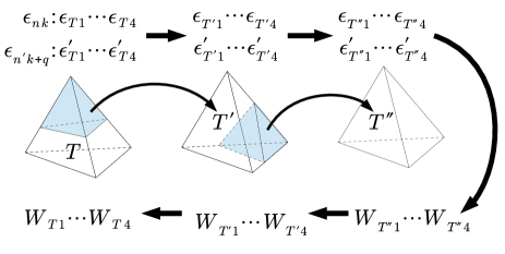
Figure 7: Flow of the calculation of weights. We divide the tetrahedra two times to cut out regions where two Heaviside functions become one.

Appendix B How to divide a tetrahedron

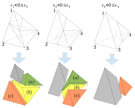
Figure 8: How to divide a tetrahedron in the case of $\epsilon_{1}\leq 0<\epsilon_{2}$ (left), $\epsilon_{2}\leq 0<\epsilon_{3}$ (center), and $\epsilon_{3}\leq 0<\epsilon_{4}$ (right).

We will explain how to cut out tetrahedra $T^{\prime}$ in the case of $\theta(\epsilon)=1$ from tetrahedron $T$. We represent $\epsilon_{nk}$ at the corners of $T$ as $\epsilon_{1},\cdots,\epsilon_{4}$, where $\epsilon_{1}\leq\epsilon_{2}\leq\epsilon_{3}\leq\epsilon_{4}$. We define $a_{ij}=-\epsilon_{j}/(\epsilon_{i}-\epsilon_{j})$. In all cases

$$V_{T^{\prime}}=V_{T}\left|\det\left(F\right)\right|.$$ (37)

1. $0\leq\epsilon_{1}$:
   We cut out no tetrahedra because $\theta(\epsilon)$ becomes 1 over the entire tetrahedron in this case.

   $$F =\begin{pmatrix}1&0&0&0\\ 0&1&0&0\\ 0&0&1&0\\ 0&0&0&1\end{pmatrix}$$ (38)

2. $\epsilon_{1}\leq 0<\epsilon_{2}$:
   Three tetrahedra are cut out (Fig. 8 left).

   $$(a)\qquad F =\begin{pmatrix}a_{12}&a_{21}&0&0\\ a_{13}&0&a_{31}&0\\ a_{14}&0&0&a_{41}\\ 0&0&0&1\end{pmatrix}$$ (39)

   $$(b)\qquad F =\begin{pmatrix}a_{12}&a_{21}&0&0\\ a_{13}&0&a_{31}&0\\ 0&0&1&0\\ 0&0&0&1\end{pmatrix}$$ (40)

   $$(c)\qquad F =\begin{pmatrix}a_{12}&a_{21}&0&0\\ 0&1&0&0\\ 0&0&1&0\\ 0&0&0&1\end{pmatrix}$$ (41)

3. $\epsilon_{2}\leq 0<\epsilon_{3}$:
   Three tetrahedra are cut out (Fig. 8 center).

   $$(a)\qquad F =\begin{pmatrix}a_{13}&0&a_{31}&0\\ a_{14}&0&0&a_{41}\\ 0&a_{24}&0&a_{42}\\ 0&0&0&1\end{pmatrix}$$ (42)

   $$(b)\qquad F =\begin{pmatrix}a_{13}&0&a_{31}&0\\ 0&a_{23}&a_{32}&0\\ 0&a_{24}&0&a_{42}\\ 0&0&0&1\end{pmatrix}$$ (43)

   $$(c)\qquad F =\begin{pmatrix}a_{13}&0&a_{31}&0\\ 0&a_{23}&a_{32}&0\\ 0&0&1&0\\ 0&0&0&1\end{pmatrix}$$ (44)

4. $\epsilon_{3}\leq 0<\epsilon_{4}$:
   One tetrahedron is cut out (Fig. 8 right).

   $$F =\begin{pmatrix}a_{14}&0&0&a_{41}\\ 0&a_{24}&0&a_{42}\\ 0&0&a_{34}&a_{43}\\ 0&0&0&1\end{pmatrix}$$ (45)

Appendix C Calculation of $W^{(1)}_{T^{\prime\prime}}$

We represent the matrix elements at the corners of the tetrahedron as $f_{1},\cdots,f_{4}$. We evaluate the integral

$$\Braket{\frac{A}{d}}_{T^{\prime\prime}}=\int_{T^{\prime\prime}}d^{3}k\frac{A_{\bm{k}}}{d_{\bm{k}}}$$ (46)

using linear interpolation to obtain

$$A_{T^{\prime\prime}}\approx 6V^{\prime\prime}\int^{1}_{0}dx\int_{0}^{1-x}dy\int_{0}^{1-x-y}dz$$

$$\times\frac{A_{1}+(A_{2}-A_{1})x+(A_{3}-A_{1})y+(A_{4}-A_{1})z}{d_{1}+(d_{2}-d_{1})x+(d_{3}-d_{1})y+(d_{4}-d_{1})z}$$

$$\equiv \sum_{i=1}^{4}A_{i}W_{T^{\prime\prime}i},$$ (47)

where

$$W_{T^{\prime\prime}i}=6V^{\prime\prime}\int_{0}^{1} dx_{1}\int^{1}_{0}dx_{2}\int_{0}^{1}dx_{3}\int_{0}^{1}dx_{4}$$

$$\times\frac{x_{i}\delta(x_{1}+x_{2}+x_{3}+x_{4}-1)}{d_{1}x_{1}+d_{2}x_{2}+d_{3}x_{3}+d_{4}x_{4}}.$$ (48)

This in turn yields (33).

References

- Hohenberg and Kohn (1964) P. Hohenberg and W. Kohn, Phys. Rev. 136, B864 (1964).
- Perdew et al. (1996) J. Perdew, M. Emzerhof, and K. Burke, J. Chem. Phys. 105, 9982 (1996).
- Hedin (1965) L. Hedin, Phys. Rev. 139, A796 (1965).
- Methfessel and Paxton (1989) M. Methfessel and A. T. Paxton, Phys. Rev. B 40, 3616 (1989).
- Jepsen and Andersen (1971) O. Jepsen and O. K. Andersen, Solid State Commun. 9, 1763 (1971).
- Rath and Freeman (1975) J. Rath and A. J. Freeman, Phys. Rev. B 11, 2109 (1975).
- Savrasov (1992) S. Y. Savrasov, Phys. Rev. Lett. 69, 2819 (1992).
- Savrasov and Savrasov (1996) S. Y. Savrasov and D. Y. Savrasov, Phys. Rev. B 54, 16487 (1996).
- Fujiwara et al. (2003) T. Fujiwara, S. Yamamoto, and Y. Ishii, J. Phys. Soc. Jpn. 72, 777 (2003).
- Blöchl et al. (1994) P. E. Blöchl, O. Jepsen, and O. K. Andersen, Phys. Rev. B 49, 16223 (1994).
- Baroni et al. (2001) S. Baroni, S. de Gironcoli, A. Dal Corso, and P. Giannozzi, Rev. Mod. Phys. 73, 515 (2001).
- Calandra et al. (2010) M. Calandra, G. Profeta, and F. Mauri, Phys. Rev. B 82, 165111 (2010).
- Bazhirov et al. (2010) T. Bazhirov, J. Noffsinger, and M. L. Cohen, Phys. Rev. B 82, 184509 (2010).
- Giannozzi et al. (2009) P. Giannozzi, S. Baroni, N. Bonini, M. Calandra, R. Car, C. Cavazzoni, D. Ceresoli, G. L. Chiarotti, M. Cococcioni, I. Dabo, A. Dal Corso, S. de Gironcoli, S. Fabris, G. Fratesi, R. Gebauer, U. Gerstmann, C. Gougoussis, A. Kokalj, M. Lazzeri, L. Martin-Samos, N. Marzari, F. Mauri, R. Mazzarello, S. Paolini, A. Pasquarello, L. Paulatto, C. Sbraccia, S. Scandolo, G. Sclauzero, A. P. Seitsonen, A. Smogunov, P. Umari, and R. M. Wentzcovitch, J. Phys.: Condens. Matter 21, 395502 (2009).
- Nagamatsu et al. (2001) J. Nagamatsu, N. Nakagawa, T. Muranaka, Y. Zenitani, and J. Akimitsu, Nature (London) 410, 63 (2001).
- Kong et al. (2001) Y. Kong, O. V. Dolgov, O. Jepsen, and O. K. Andersen, Phys. Rev. B 64, 020501 (2001).
- Bohnen et al. (2001) K.-P. Bohnen, R. Heid, and B. Renker, Phys. Rev. Lett. 86, 5771 (2001).
- Choi et al. (2002) H. J. Choi, D. Roundy, H. Sun, M. L. Cohen, and S. G. Louie, Phys. Rev. B 66, 020513 (2002).
- Eiguren and Ambrosch-Draxl (2008) A. Eiguren and C. Ambrosch-Draxl, Phys. Rev. B 78, 045124 (2008).
- Hanfland et al. (2000) M. Hanfland, K. Syassen, N. Christensen, and D. Novikov, Nature (London) 408, 174 (2000).
- Deemyad and Schilling (2003) S. Deemyad and J. S. Schilling, Phys. Rev. Lett. 91, 167001 (2003).
- Struzhkin et al. (2002) V. Struzhkin, M. Eremets, W. Gan, H. Mao, and R. Hemley, Science 298, 1213 (2002).
- Shimizu et al. (2002) K. Shimizu, H. Ishikawa, D. Takao, T. Yagi, and K. Amaya, Nature (London) 419, 597 (2002).
- Hamann et al. (1979) D. R. Hamann, M. Schlüter, and C. Chiang, Phys. Rev. Lett. 43, 1494 (1979).
- Vanderbilt (1990) D. Vanderbilt, Phys. Rev. B 41, 7892 (1990).
- (26) We used the pseudopotential Li.pbe-s-rrkjus_psl.0.2.1.UPF from http://www.quantum-espresso.org.
- Perdew et al. (1997) J. P. Perdew, K. Burke, and M. Ernzerhof, Phys. Rev. Lett. 78, 1396 (1997).
- de Gironcoli (1995) S. de Gironcoli, Phys. Rev. B 51, 6773 (1995).
- McMillan (1968) W. L. McMillan, Phys. Rev. 167, 331 (1968).
- Dynes (1972) R. Dynes, Solid State Commun. 10, 615 (1972).
- Oliveira et al. (1988) L. N. Oliveira, E. K. U. Gross, and W. Kohn, Phys. Rev. Lett. 60, 2430 (1988).
- Lüders et al. (2005) M. Lüders, M. A. L. Marques, N. N. Lathiotakis, A. Floris, G. Profeta, L. Fast, A. Continenza, S. Massidda, and E. K. U. Gross, Phys. Rev. B 72, 024545 (2005).