Difference-in-Differences for Policy Evaluation

Abstract

Difference-in-differences is one of the most used identification strategies in empirical work in economics. This chapter reviews a number of important, recent developments related to difference-in-differences. First, this chapter reviews recent work pointing out limitations of two way fixed effects regressions (these are panel data regressions that have been the dominant approach to implementing difference-in-differences identification strategies) that arise in empirically relevant settings where there are more than two time periods, variation in treatment timing across units, and treatment effect heterogeneity. Second, this chapter reviews recently proposed alternative approaches that are able to circumvent these issues without being substantially more complicated to implement. Third, this chapter covers a number of extensions to these results, paying particular attention to (i) parallel trends assumptions that hold only after conditioning on observed covariates and (ii) strategies to partially identify causal effect parameters in difference-in-differences applications in cases where the parallel trends assumption may be violated.

JEL Codes:

C14, C21, C23

Keywords:

Difference-in-differences, policy evaluation, panel data, treatment effect heterogeneity, parallel trends, two way fixed effects, event study

1 Introduction

This chapter reviews a number of recent contributions related to difference-in-differences (DID) approaches to evaluate economic policies. Difference-in-differences approaches are extremely popular in applied work in economics, and difference-in-differences methodology features prominently in well known textbooks such as [3, 38]. Although difference-in-differences identification strategies have been popular in empirical work for roughly the past 30 years ([30, 31]), there has been renewed interest in methodological issues related to difference-in-differences approaches in recent years. This interest stems from several highly influential papers that have pointed out potentially severe weaknesses with the two way fixed effects (TWFE) regressions that have been the primary way that DID identification strategies have been implemented ([63, 41, 14, 50, 76, 8, 57]). One of the main goals of this chapter is to summarize these papers as well as to review a number of recently proposed approaches that are able to circumvent the limitations of TWFE regressions.

Before proceeding along these lines, it is worth fixing ideas on what exactly DID is as well as pointing out some peculiarities of DID identification strategies. First, DID identification strategies involve observing some units in some period(s) before they become treated as well as in some period(s) after they become treated — collectively, these units are referred to as the “treated group.” Observing some units in time periods before and after they become treated is a particularly powerful framework for learning about causal effects. This is arguably the reason that DID identification strategies are often included among “natural experiment” methods in economics and is a primary difference relative to traditional panel data approaches in economics.

Second, difference-in-differences strategies typically focus on identifying and estimating the Average Treatment Effect on the Treated (ATT); this is exactly the average effect of the treatment among those who switch from being untreated to being treated. The ATT is equal to the average path of outcomes experienced over time by the treated group relative to the average path of outcomes that the treated group would have experienced had it not participated in the treatment. Thus, the key identification challenge in DID applications is recovering this “counterfactual” path of outcomes for the treated group. The main identifying assumption underlying DID is called the parallel trends assumption. It says that, in the absence of participating in the treatment, the counterfactual path of outcomes for the treated group is the same as the path of outcomes that the “untreated group” (the group of units that did not participate in the treatment) actually experienced. Third, DID identification strategies allow for treatment effect heterogeneity; that is, that the effect of participating in the treatment can vary across units (within time periods), across time periods, and across length of exposure to the treatment.

The dominant approach to implementing DID identification strategies has been to use two-way fixed effects (TWFE) regressions. The simplest and most common version of this approach is the following regression

$$Y_{it}=\theta_{t}+\eta_{i}+\alpha D_{it}+v_{it}$$ (1)

where $Y_{it}$ is the outcome of interest, $\theta_{t}$ is a time fixed effect, $\eta_{i}$ is a unit fixed effect, $D_{it}$ is an indicator for whether or not unit $i$ participated in the treatment in time period $t$, and $v_{it}$ are idiosyncratic, time-varying unobservables.

Under treatment effect homogeneity (and under the parallel trends assumption), $\alpha$ in the TWFE regression is equal to the causal effect of participating in the treatment. However, in cases with treatment effect heterogeneity, researchers have often (loosely) interpreted $\alpha$ as an overall average treatment effect. That a TWFE regression delivers a single summary measure of the effect of the treatment is appealing in many applications. Unfortunately, this kind of TWFE regression is not generally robust to treatment effect heterogeneity ([50, 41, 14]). Section 3 discusses these issues extensively, but a rough intuition is that researchers ask “too much” out of a TWFE regression; that is, they ask the TWFE regression to both allow for treatment effect heterogeneity and to fully summarize the causal effect of participating in the treatment into a single number $\alpha$, but the TWFE regression can only do one of these. [50] provides an alternative explanation for the non-robustness of TWFE regressions to treatment effect heterogeneity: $\alpha$ can be shown to be equal to a weighted average of underlying comparisons of paths of outcomes among groups whose treatment status changes relative to groups whose treatment status remains the same across time periods. These comparisons include both (i) using groups that are not-yet-treated as the comparison group and (ii) using groups that were treated in previous periods as the comparison group. The first comparison is exactly the type of comparison that should be used in DID applications, but the second type of comparison (sometimes called “bad comparisons” or “forbidden comparisons”) is generally not desirable in applications and can lead to poor estimates of causal effect parameters, particularly in the presence of treatment effect dynamics. Even in cases without treatment effect dynamics, the weights on underlying treatment effect parameters are still (undesirably) driven by the estimation method which can lead to estimates of overall treatment effects being different from the actual overall treatment effect. Both of these issues open up the possibility of poor estimates of causal effect parameters due to the estimation strategy, even when the identification strategy is valid. These are major weaknesses of using TWFE regressions in this context.

One of the main contributions of recent work on DID is to more clearly separate identification and estimation. In particular, following [29], the current chapter defines group-time average treatment effects, $ATT(g,t)$, to be the average treatment effect for a particular group at a particular point in time; a leading example of a group is to define it by the time period when a unit first becomes treated. The group-time average treatment effect is a natural generalization of the $ATT$ from the case with two time periods to the case with more time periods and variation in treatment timing. Identification arguments for group-time average treatment effects are essentially analogous to identification arguments for the $ATT$ in the two period case, and identification holds under the parallel trends assumptions without requiring additional assumptions restricting treatment effect heterogeneity. Group-time average treatment effects can provide important information about treatment effect heterogeneity with respect to group and time period and/or length of exposure to the treatment. Perhaps more importantly, group-time average treatment effects can play the role of a building-block for more aggregated treatment effect parameters. For example, if desired by the researcher, they can be aggregated into alternative target parameters such as an overall $ATT$ parameter or into an event study.

Interestingly, the usefulness of the strategy of identifying group-time average treatment effects in the presence of multiple time periods, variation in treatment timing, and treatment effect heterogeneity applies much more broadly than just to DID applications. In particular, this strategy provides a path to extending any sort of identification arguments from the case without variation in treatment timing to cases with more time periods and variation in treatment timing. See Remark 2 below for additional discussion along these lines.

Another main goal of this chapter is to compare some of the main new approaches to estimating causal effect parameters that have been proposed recently proposed; this chapter mainly considers the approach proposed in [29], the “imputation” approaches proposed in [60, 48, 14], and the regression approaches proposed in [76, 77]. All of these procedures follow similar high-level strategies: in a first step, they explicitly make the same “good comparisons” that show up in the TWFE regression (i.e., the comparisons that use units that become treated relative to units that are not-yet-treated) while explicitly avoiding the “bad comparisons” that show up in the TWFE regression (i.e., the comparisons that use already-treated units as the comparison group). Then, in a second step, they combine these underlying treatment effect parameters into target parameters of interest such as an overall average treatment effect on the treated or into an event study. This discussion suggests a high degree of similarity between all of these approaches. That being said, these approaches typically do not lead to exactly the same estimates of causal effect parameters (except in a few special cases). One main reason for this is different default choices in the software implementations of different procedures. To my knowledge, there are perhaps only two meaningful differences between approaches. In cases where the parallel trends assumption includes covariates, the doubly robust approach in [29] generally imposes weaker functional form requirements on the way covariates enter the model than alternative approaches; moreover, these types of identification arguments can be connected to the literature on double/de-biased machine learning (e.g., [35, 34]) which could further substantially weaken functional form requirements with respect to observed covariates. On the other hand, imputation strategies are often very convenient to implement in that they only involve estimating panel data-type regressions and computing predicting values. This is an important advantage particularly in “non-standard” setups. That being said, even these differences are arguably second order relative to the first order issues with TWFE regressions that all of these approaches address.

Next, the chapter turns to two useful extensions of the previous results. The first extension is to the case where the parallel trends assumption holds only after conditioning on some covariates. To give a simple example where conditioning on covariates in the parallel trends assumption is useful, consider a labor economist interested in the effect of some treatment on a person’s earnings. In this type of application, it seems likely that paths of earnings (in the absence of participating in the treatment) depend on things like demographic characteristics and years of education. If these variables are distributed differently among the treated and untreated group, then the “unconditional” parallel trends assumptions considered so far are generally violated. The new approaches to DID discussed above can readily accommodate including covariates in the parallel trends assumption; moreover, the chapter further reviews the case where the covariates may themselves be affected by participating in the treatment (sometimes referred to as a “bad control” problem) and discusses recent methodological innovations in this context as well.

The second extension is for the case where parallel trends is violated (even after potentially conditioning on covariates). It is important to emphasize that the parallel trends assumption does not hold automatically in applications with repeated observations over time. The most common way to rationalize the parallel trends assumption is using the following model for untreated potential outcomes

$$Y_{it}(0)=\theta_{t}+\eta_{i}+v_{it}$$ (2)

where $Y_{it}(0)$ denotes unit $i$’s untreated potential outcome in time period $t$ — this is the outcome that unit $i$ would have experienced in time period $t$ if it had not participated in the treatment, $\theta_{t}$ is a time fixed effect, $\eta_{i}$ is an individual fixed effect that can follow a different distribution for the treated group relative to the untreated group, and $v_{it}$ are (idiosyncratic) time varying unobservables (see, for example, [12, 48, 14]). There are a number of attractive features of this model. First, it does not put any structure on how untreated potential outcomes are generated at all. Second, it allows for arbitrary treatment effect heterogeneity. Third, units can select into the treatment on the basis of their treated potential outcomes or on their time invariant unobservables that affect untreated potential outcomes, $\eta_{i}$, but not on the basis of the time varying unobservables, $v_{it}$.

Besides these, many economic models involve unobserved heterogeneity (like $\eta_{i}$) that may be distributed differently between the treated group and the untreated group as well as trends in outcomes over time (like $\theta_{t}$). However, the parallel trends assumption also relies heavily on the additive separability between the time and individual effects; this additive separability is often not explicitly implied by economic theory. And, in many cases, it seems like it would be hard for researchers to ex ante evaluate its validity. Therefore, the chapter also emphasizes recent contributions from [61, 66] related to bounding treatment effects in a DID setup. Roughly, the idea of these papers is to consider how large violations of parallel trends assumptions can be before the results in post-treatment periods break down. One general challenge in the sensitivity analysis literature is that it is often not clear what constitutes a “large” amount of robustness to violations of underlying assumptions. However, DID applications, particularly those with additional pre-treatment time periods, are particularly attractive in this context because the magnitude of treatment effects in post-treatment time periods can be compared to the size of violations of parallel trends in pre-treatment time periods.

To conclude, the chapter provides an application on the minimum wage and employment as a way to illustrate the methodological points. This application comes from (and expands) the application in [29]. The application focuses on a period from 2001-2007 where the federal minimum wage was constant over time and uses changes in state-level minimum wage policies over time to identify effects of minimum wage increases on employment among teenagers. This example is merely intended to be illustrative of the methodological issues discussed in this chapter, and there are some notable weaknesses (discussed in more detail below). That said, the point of the application is to illustrate the empirical relevance of new approaches to DID in a relatively realistic application. Broadly, there are three main takeaways from the application. First, while the results from using traditional TWFE and event study regressions are not radically different from the results using new approaches, they are different enough to suggest that researchers should prefer using the new methods. Second, the new approaches all impose that the researcher make a number of good choices in the context of DID (such as not including units that are already treated in the first period or including time periods after all units become treated). While TWFE regressions can still suffer from negative weights and weights undesirably driven the estimation in this case, making these same sorts of “good choices” tends to notably improve the performance of regression-based estimation strategies. Finally, it is important to emphasize that the new approaches all still rely on the validity of the parallel trends assumption. Combining the [66] sensitivity analysis with new approaches to DID turns out to be very useful in this application as there appear to be moderately-sized violations of parallel trends in pre-treatment periods.

2 Baseline Case: Two Periods and Two Groups

This section considers the simplest, “textbook” version of DID — the case where there are exactly two time periods, where no units are treated in the first time periods, and where some units (the treated group) become treated in the second time period while other units (the untreated group) remain untreated in the second time period.

Notation:

This section uses the following notation. Denote the two time periods by $t^{*}$ and $t^{*}-1$ and define a treatment indicator $D_{i}$, so that $D_{i}=1$ for units that participate in the treatment and $D_{i}=0$ for units that do not participate in the treatment. Next, for $t\in\{t^{*}-1,t^{*}\}$, define $Y_{it}(1)$ to be unit $i$’s treated potential outcome in time period $t$ (this is the outcome that it would experience if it were in the treated group), and define $Y_{it}(0)$ to be unit $i$’s untreated potential outcome in time period $t$ (this is the outcome that it would experience if it were in the untreated group). The next condition is that $Y_{it^{*}-1}(1)=Y_{it^{*}-1}(0)$ for all units. This is a no-anticipation condition (which is discussed more carefully in the next section) which rules out the treatment affecting outcomes in periods before the treatment takes place. Under these conditions, the observed outcomes in each time period are $Y_{it^{*}-1}=Y_{it^{*}-1}(0)$ and $Y_{it^{*}}=D_{i}Y_{it^{*}}(1)+(1-D_{i})Y_{it^{*}}(0)$. In other words, in the first time period, one observes untreated potential outcomes for all units; and in the second time period, one observes treated potential outcomes for treated units and untreated potential outcomes for untreated units.

Target Parameters:

Most commonly, DID identification strategies target the average treatment effect on the treated (ATT), which is defined as:

$$ATT=\mathbb{E}[Y_{t^{*}}(1)-Y_{t^{*}}(0)|D=1]$$

The ATT is the mean difference between treated and untreated potential outcomes among the treated group. Perhaps a main reason that the DID literature most often considers identifying the ATT rather than, say, the ATE is that, for the treated group, the researcher observes untreated potential outcomes (in pre-treatment time periods) and treated potential outcomes (in post-treatment time periods). DID identification strategies exploit this framework, and, therefore, it is natural to identify causal effect parameters that are local to the treated group.

Identification:

The main identifying assumption underlying the DID approach is the parallel trends assumption, which in the case with two time periods, is given by

Assumption 1 (Parallel Trends).

$$\mathbb{E}[\Delta Y_{t^{*}}(0)|D=1]=\mathbb{E}[\Delta Y_{t^{*}}(0)|D=0]$$

As discussed in the introduction, Assumption 1 says that the path of untreated potential outcomes is, on average, the same between the treated group and the untreated group. This seems immediately useful from an identification standpoint because the path of untreated potential outcomes is not observed for the treated group, but the path of untreated potential outcomes is observed for units in the untreated group. In fact, this assumption is strong enough to identify $ATT$. To see this, notice that

$$ATT =\mathbb{E}[Y_{t^{*}}(1)-Y_{t^{*}}(0)|D=1]$$

$$=\mathbb{E}[Y_{t^{*}}(1)-Y_{t^{*}-1}(0)|D=1]-\mathbb{E}[Y_{t^{*}}(0)-Y_{t^{*}-1}(0)|D=1]$$

$$=\mathbb{E}[\Delta Y_{t^{*}}|D=1]-\mathbb{E}[\Delta Y_{t^{*}}(0)|D=1]$$

$$=\mathbb{E}[\Delta Y_{t^{*}}|D=1]-\mathbb{E}[\Delta Y_{t^{*}}(0)|D=0]$$

$$=\mathbb{E}[\Delta Y_{t^{*}}|D=1]-\mathbb{E}[\Delta Y_{t^{*}}|D=0]$$ (3)

where the first equality comes from the definition of $ATT$, the second equality holds by adding and subtracting $\mathbb{E}[Y_{t^{*}-1}(0)|D=1]$, the third equality holds because $Y_{t^{*}}(1)$ and $Y_{t^{*}-1}(0)$ are observed outcomes for the treated group, the fourth equality uses the parallel trends assumption, and the last equality holds because $\Delta Y_{t^{*}}(0)$ corresponds to the observed path of outcomes for units in the untreated group.

The expression in Equation 3 implies that $ATT$ is identified under Assumption 1, and the particular expression on the right hand side of Equation 3 is where difference-in-differences gets its name. Under parallel trends, $ATT$ is equal to the average difference in outcomes over time for the treated group adjusted by the average difference in outcomes over time for the untreated group. An alternative intuition for the expression in Equation 3 is the following: The researcher observes the path of outcomes over time for the treated group. The parallel trends assumption says that one can obtain the path of outcomes that the treated group would have experienced if they had not participated in the treatment from the untreated group. Therefore, the $ATT$ is equal to the actual path of outcomes experienced by the treated group adjusted by the path of outcomes of the untreated group. As an additional remark, notice that the above arguments have not imposed any assumptions restricting treatment effect heterogeneity.

Estimation:

The expression in Equation 3 immediately suggests an estimator for $ATT$ by replacing population means with sample averages given by

$$\widehat{ATT}=\frac{1}{n_{1}}\sum_{i=1}^{n}D_{i}\Delta Y_{it^{*}}-\frac{1}{n_{0}}\sum_{i=1}^{n}(1-D_{i})\Delta Y_{it^{*}}$$ (4)

where $n_{1}$ is the number of treated observations and $n_{0}$ is the number of untreated observations. Rather than taking this approach, most often $ATT$ is estimated using the TWFE regression in Equation 1. In the case considered in this section with exactly two periods, this regression is exactly equivalent to the simple linear regression of $\Delta Y_{it^{*}}$ on $D_{i}$ given by

$$\Delta Y_{it^{*}}=\theta^{*}_{t^{*}}+\alpha D_{i}+\Delta v_{it^{*}}$$ (5)

where $\theta^{*}_{t^{*}}:=(\theta_{t^{*}}-\theta_{t^{*}-1})$.

Interestingly, although the regression above appears to have restricted the effect of participating in the treatment to be constant (and given by $\alpha$) across all units, it is straightforward to show that in this case

$$\alpha=\mathbb{E}[\Delta Y_{t^{*}}|D=1]-\mathbb{E}[\Delta Y_{t^{*}}|D=0]=ATT$$

and, likewise, that

$$\hat{\alpha}=\widehat{ATT}$$

In other words, in the case with exactly two time periods, the TWFE regression is robust to treatment effect heterogeneity. The regression in Equation 5 is as straightforward to estimate as the averages in Equation 4. Moreover, this regression provides a convenient way to recover standard errors and to conduct inference using standard statistical software. The combination of robustness and simplicity of the TWFE regression in this case provides an explanation for its popularity.

Finally, and at the risk of belaboring the point, it is also worth mentioning how to estimate $ATT$ using an imputation approach in this relatively simple setting (this is instructive for the more complicated cases considered in the next section). Imputation estimators work by estimating the model for untreated potential outcomes in Equation 2 using all available untreated observations. Because the researcher does not observe untreated potential outcomes for the treated group, after taking first differences (or making a within transformation — which are equivalent in this case), this amounts to the regression

$$\Delta Y_{it^{*}}(0)=\theta_{t^{*}}+\Delta v_{it^{*}}$$

using observations from the untreated group and which, for simplicity, imposes the normalization that $\theta_{t^{*}-1}=0$. In this case, $\hat{\theta}_{t^{*}}=\frac{1}{n_{0}}\sum_{i=1}^{n}(1-D_{i})\Delta Y_{it^{*}}$. Furthermore, $Y_{it^{*}}(0)$ can be “imputed” for the treated group using

$$\hat{Y}_{it^{*}}(0)=Y_{it^{*}-1}+\hat{\theta}_{t^{*}}$$

and, therefore,

$$\widehat{ATT}_{imp} =\frac{1}{n_{1}}\sum_{i=1}^{n}D_{i}(Y_{it^{*}}-\hat{Y}_{it^{*}}(0))$$

$$=\frac{1}{n_{1}}\sum_{i=1}^{n}D_{i}\big{(}Y_{it^{*}}-(Y_{it^{*}-1}-\hat{\theta}_{t^{*}})\big{)}$$

$$=\frac{1}{n_{1}}\sum_{i=1}^{n}D_{i}\Delta Y_{it^{*}}-\frac{1}{n_{0}}\sum_{i=1}^{n}(1-D_{i})\Delta Y_{it^{*}}$$

$$=\widehat{ATT}$$

This discussion suggests that, estimating ATT by (i) the sample analogue of Equation 3, (ii) TWFE regression, or (iii) imputation, all result in numerically identical estimates in the textbook case for DID with exactly two time periods. The next section shows that this equivalence is lost when one considers more complicated cases with more periods and variation in treatment timing.

3 Multiple Periods and Variation in Treatment Timing

Much of the recent difference-in-differences literature has been interested in questions surrounding how well DID identification and estimation strategies scale to settings where there are more than two time periods and there is variation in treatment timing. These sorts of cases are often encountered in applied work. This section primarily covers (i) several recent results on the limitations of TWFE regressions to implement DID identification strategies and (ii) a number of recently suggested approaches that can circumvent the limitations that TWFE regressions suffer from. To fix ideas, this section primarily focuses on the staggered treatment adoption case as in the following assumption.

Assumption 2 (Staggered Treatment Adoption).

For all units and for all $t=2,\ldots,\mathcal{T}$, $D_{it-1}=1\implies D_{it}=1$.

Staggered treatment adoption means that once a unit becomes treated, that unit remains treated in future time periods. Staggered treatment adoption occurs in applications where different locations implement policies at different points in time (and then those policies remain in place). Staggered treatment adoption also applies in many applications where the unit is not literally treated over and over across periods, but rather that treatment is “scarring”. For example, researchers studying the effects of job training programs typically categorize individuals as being treated at the first time they participate in job training and in all subsequent periods (see, [76] for more discussion along these lines).

Notation:

This section extends the notation from the previous section. Now consider a case with $\mathcal{T}$ time periods and with staggered treatment adoption. Towards this end, define groups by the time period when a unit first becomes treated; for a particular unit, let $G_{i}$ indicate its group and denote the set of all groups by $\mathcal{G}\subseteq\{2,\ldots,\mathcal{T},\mathcal{T}+1\}$. Further, define $\bar{\mathcal{G}}=\mathcal{G}\setminus\{\mathcal{T}+1\}$ which is the set of groups excluding the never-treated group. Under staggered treatment adoption, knowing a unit’s group implies that the researcher knows its entire path of participating in the treatment across all time periods. For units that do not participate in the treatment, arbitrarily set their group to be $\mathcal{T}+1$ (which somewhat lessens the notational burden for a few lines of algebra in the next section but is otherwise inconsequential). It is also convenient to define the variable $U_{i}$ that is equal to 1 for units in the “never-treated” group and is otherwise equal to 0 for units that ever participate in the treatment. Next, define potential outcomes by a unit’s group; in particular, $Y_{it}(g)$ is the outcome that unit $i$ would experience in time period $t$ if it became treated in period $g$. Also, continue to denote $Y_{it}(0)$ as the potential outcome that unit $i$ would experience in time period $t$ if it did not participate in the treatment in any time period.

Assumption 3 (No Anticipation).

For all units $i$ and time period $t<G_{i}$ (pre-treatment time periods), $Y_{it}=Y_{it}(0)$.

Assumption 3 says that participating in the treatment does not have an effect on a unit’s outcomes in time periods before the treatment actually occurs. In some applications, it could be the case that some units anticipate being treated and “make adjustments” that affect their outcomes in periods before the treatment takes place. It is relatively straightforward to accommodate anticipation in a DID framework; in particular, one can essentially “back up” the analysis far enough in time and only include as pre-treatment periods those periods that are “far enough” before the treatment actually begins (see, for example, [29, 76]). For simplicity, this chapter mostly ignores issues related to violations of the anticipation condition above.

Under Assumption 3, observed outcomes are given by $Y_{it}=Y_{it}(0)$ when $t<G_{i}$ and $Y_{it}=Y_{it}(G_{i})$ when $t\geq G_{i}$. In other words, in pre-treatment periods, the researcher observes untreated potential outcomes, and, in post-treatment periods, the researcher observes potential outcomes corresponding to the unit’s actual group.

The next assumption provides an extended version of the parallel trends assumption to accommodate multiple time periods and variation in treatment timing.

Assumption 4 (Parallel Trends for Multiple Periods and Variation in Treatment Timing).

For all $t=2,\ldots,\mathcal{T}$, and for all $g\in\mathcal{G}$,

$$\mathbb{E}[\Delta Y_{t}(0)|G=g]=\mathbb{E}[\Delta Y_{t}(0)]$$

Assumption 4 says that average paths of untreated potential outcomes are the same for all groups and all time periods. This is a natural generalization of the parallel trends assumption in Assumption 1 to the case with multiple periods and variation in treatment timing. Like that assumption, Assumption 4 allows for heterogeneous treatment effects (both across units and with respect to time and/or length of exposure to the treatment). It also does not place any restriction on treated potential outcomes at all, and it is compatible with a fixed effects model for untreated potential outcomes like the one in Equation 2 across all time periods while allowing for the distribution of the individual fixed effect, $\eta$, to arbitrarily vary across groups. That said, there are alternative versions of parallel trends assumptions that researchers could invoke here. One example that is discussed in the next section, is when parallel trends only holds among those with similar observed characteristics. Another similar (and weaker) assumption would be to assume that parallel trends only holds relative to the never treated group and only for certain time periods. See [62] for a detailed discussion and comparison of several different possible parallel trends assumptions. To give one more example, another interesting assumption is that parallel trends holds only among groups that ever participate in the treatment. This chapter focuses on the version of parallel trends in Assumption 4, but many of the approaches considered below could be implemented under alternative parallel trends assumptions with only slight modification.

Target Parameters:

There are a large number of parameters that a researcher could potentially be interested in when there are multiple periods and variation in treatment timing. This section considers three main parameters of interest: group-time average treatment effects, overall average treatment effects, and event studies; several additional parameters are considered in [29].

To start with, define group-time average treatment effects which are given by

$$ATT(g,t)=\mathbb{E}[Y_{t}(g)-Y_{t}(0)|G=g]$$

These are the average treatment effect for group $g$ in time period $t$. $ATT(g,t)$ is an important parameter in the DID literature. First, from an identification standpoint, the next section shows that $ATT(g,t)$ can be identified using essentially the same arguments as in the case with exactly two periods considered above. Second, under Assumption 4, recent work shows that $\alpha$ in the TWFE regression can be related to “underlying” $ATT(g,t)$’s. Third, $ATT(g,t)$ can be used to highlight treatment effect heterogeneity with respect to group, time period, and/or length of exposure to the treatment. In some applications, the number of group-time average treatment effects may be large (e.g., this happens when the number of groups and time periods is relatively large) and, therefore, may be challenging to report and/or interpret. $ATT(g,t)$’s can also serve as the building block for more aggregated treatment effect parameters.

Towards this end, among units that ever participate in the treatment, define $\overline{TE}_{i}:=\frac{1}{\mathcal{T}-G_{i}+1}\displaystyle\sum_{t=G_{i}}^{\mathcal{T}}\big{(}Y_{it}-Y_{it}(0)\big{)}$, which is the average treatment effect for unit $i$ across all of its post-treatment time periods. One version of an overall treatment effect parameter is

$$ATT^{O}=\mathbb{E}\left[\overline{TE}|G\leq\mathcal{T}\right]$$

where conditioning on $G\leq\mathcal{T}$ amounts to conditioning on becoming treated in any period from $t=2,\ldots,\mathcal{T}$. This is a natural analogue for $ATT$ in the case with multiple periods and variation in treatment timing. It is the average effect of participating in the treatment among those that participate in the treatment across all their post-treatment time periods. Like the coefficient on $D_{it}$ in a TWFE regression, $ATT^{O}$ is a single number; it can be used to summarize the causal effect of participating in the treatment among those that ever participated. [29] show that

$$ATT^{O}=\sum_{g\in\mathcal{G}}\sum_{t=2}^{\mathcal{T}}w^{O}(g,t)ATT(g,t)$$

where

$$w^{O}(g,t)=\textrm{P}(G=g|G\leq\mathcal{T})\frac{\mathbf{1}\{t\geq g\}}{\mathcal{T}-g+1}$$

That is, $ATT^{O}$ can be recovered as a weighted average of $ATT(g,t)$ where the weights depend on (i) the relative size of the group among all groups that ever participate in the treatment (from the term $\textrm{P}(G=g|G\leq\mathcal{T}))$, and (ii) the number of post-treatment time periods for a particular group (from the second term) which arises due to $ATT^{O}$ applying equal weight across all treated units.

Another common target parameter in DID applications are event study parameters that summarize the effect of participating in the treatment at different lengths of exposure to the treatment. In particular, among units such that $G_{i}+e\in\{2,\ldots,\mathcal{T}\}$, define $TE_{i}(e)=\big{(}Y_{iG_{i}+e}-Y_{iG_{i}+e}(0)\big{)}$; this is the causal effect of the treatment $e$ periods after exposure to the treatment (this notation uses the convention in the literature of having $e=0$ in the period where the treatment occurs). One can summarize treatment effects across different lengths of exposure using the following parameter

$$ATT^{ES}(e)=\mathbb{E}\big{[}TE(e)|G+e\in[2,\mathcal{T}],G\leq\mathcal{T}\big{]}$$

That is, $ATT^{ES}(e)$ is the average treatment effect among those that have been exposed for exactly $e$ periods conditional on being observed having participated in the treatment for that number of periods (the condition that $G+e\in[2,\mathcal{T}]$) and ever-participating in the treatment ($G\leq\mathcal{T}$). [29] show that $ATT^{ES}(e)$ can be recovered from underlying group-time average treatment effects; in particular,

$$ATT^{ES}(e)=\sum_{g\in\mathcal{G}}w^{ES}(g,e)ATT(g,g+e)$$

where

$$w^{ES}(g,e)=\mathbf{1}\{g+e\leq\mathcal{T}\}\textrm{P}(G=g|G+e\leq\mathcal{T})$$

Thus, $ATT^{ES}(e)$ can be recovered as a weighted average of underlying $ATT(g,t)$’s. This average is given by collecting $ATT(g,t)$’s that satisfy $t=g+e$ (i.e., finding the period for a particular group where it has been exposed to the treatment for exactly $e$ periods) and then by weighting by the relative size of the group (among those groups that are ever observed to participate in the treatment for exactly $e$ periods).

Remark 1.

Given that $ATT^{O}$ and $ATT^{ES}(e)$ can be recovered from underlying $ATT(g,t)$’s, the identification arguments below focus on $ATT(g,t)$.

Remark 2.

Another notable feature of the discussion in this section is that these arguments apply quite generally for identifying causal effect parameters in applications with multiple time periods. In particular, the identification arguments below focus on identifying $ATT(g,t)$ in a DID context. However, in cases where a researcher wanted to use some other identification strategy besides DID, given that $ATT(g,t)$ is somehow identified, then the aggregations to overall treatment effect parameters, event studies, etc. continue to apply. See [26, 24] for examples along these lines in the context of unconfoundedness (conditional on lagged outcomes) and interactive fixed effects models, respectively.

3.1 Problems with TWFE Regressions

As discussed in the introduction, the dominant approach to implementing DID identification strategies has been to use the TWFE regression in Equation 1. In this context, researchers are primarily interested in $\alpha$ which has typically (though often loosely) been interpreted as an overall average treatment effect among those that ever participate in the treatment; i.e., along the lines of the definition of $ATT^{O}$ above. Recent research, particularly [63, 41, 14, 50, 8], has pointed out a number of weaknesses of this estimation strategy in cases where (i) there are more than two time periods, (ii) there is variation in treatment timing, and (iii) there is treatment effect heterogeneity — all of which are very common in applications in economics.

TWFE Regressions under Treatment Effect Homogeneity

To start with, it is worth considering where this specification comes from, and, additionally, why this approach would work well under treatment effect homogeneity. A natural starting point is the model for untreated potential outcomes in Equation 2. Next, notice that, in the setup with multiple time periods and variation in treatment timing (and under a no-anticipation condition), observed outcomes can be expressed in terms of potential outcomes by

$$Y_{it} =Y_{it}(0)+\mathbf{1}\{t\geq G_{i}\}\big{(}Y_{it}(G_{i})-Y_{it}(0)\big{)}$$ (6)

Next, a mathematical expression for treatment effect homogeneity is the condition that $Y_{it}(g)-Y_{it}(0)=\alpha$ for all units in all post-treatment time periods (i.e., periods where $t\geq g$). This condition implies that the effect of being treated does not vary across units; moreover, within units, the effect of the treatment does not vary across time periods, length of exposure, or depend on the time period when a unit becomes treated. It implies that, in post-treatment time periods, $Y_{it}(G_{i})-Y_{it}(0)=\alpha$. Plugging in the model for untreated potential outcomes in Equation 2 into Equation 6, using the treatment effect homogeneity condition, and noticing that $D_{it}=\mathbf{1}\{t\geq G_{i}\}$ implies that

$$Y_{it} =\theta_{t}+\eta_{i}+\alpha D_{it}+v_{it}$$

thus giving rise to the TWFE regression above. Under treatment effect homogeneity, the estimate of $\alpha$ from this regression can be interpreted as an estimate of the causal effect of participating in the treatment.

TWFE Regressions under Treatment Effect Heterogeneity

This section considers the same TWFE regression but relaxes the treatment effect homogeneity condition. Section 2 showed that, in the textbook case with two periods, $\alpha$ from the TWFE regression was generally robust to treatment effect heterogeneity. In contrast, this section shows that $\alpha$ is not generally robust to treatment effect heterogeneity when there are multiple periods and variation in treatment timing.

Notation:

The discussion in this section requires some extensions to the notation used so far. First, define

$$\ddot{D}_{it}:=(D_{it}-\bar{D}_{i})-\mathbb{E}[D_{t}]-\frac{1}{\mathcal{T}}\sum_{s=1}^{\mathcal{T}}\mathbb{E}[D_{s}]$$

which is the double de-meaned version of $D_{it}$. Next, for any groups $g$ and $k$, define

$$\bar{G}_{g}:=\frac{\mathcal{T}-g+1}{\mathcal{T}},\qquad\qquad p_{g}:=\textrm{P}(G=g),\qquad\qquad p_{g|\{g,k\}}:=\textrm{P}(G=g|G\in\{g,k\})$$

which are the fraction of periods for which group $g$ participates in the treatment, the overall probability of being in group $g$, and the probability of being in group $g$ conditional on either being in group $g$ or group $k$, respectively. For $t_{1}<t_{2}$, let

$$\bar{Y}_{i}^{(t_{1},t_{2})}:=\frac{1}{t_{2}-t_{1}}\sum_{t=t_{1}}^{t_{2}}Y_{it},\qquad\qquad\overline{ATT}^{(t_{1},t_{2})}(g):=\frac{1}{t_{2}-t_{1}}\sum_{t=t_{1}}^{t_{2}}ATT(g,t)$$

which are the average outcome for unit $i$ between periods $t_{1}$ and $t_{2}$ and the average group-time average treatment effect for group $g$ from period $t_{1}$ to $t_{2}$, respectively. For two groups $g$ and $k$ with $g<k$ (i.e., group $g$ becomes treated before group $k$), it is also helpful to define the short-hand notation

$$\bar{Y}_{i}^{PRE(g)}:=\bar{Y}_{i}^{(1,g-1)},\qquad\qquad\bar{Y}_{i}^{MID(g,k)}:=\bar{Y}_{i}^{(g,k-1)},\qquad\qquad\bar{Y}_{i}^{POST(k)}:=\bar{Y}_{i}^{(k,\mathcal{T})}$$

which are the average outcome for unit $i$ in periods before either group becomes treated, the average outcome for unit $i$ in periods after group $g$ becomes treated but before group $k$ becomes treated, and the average outcome for group $i$ after both group $g$ and group $k$ have become treated, respectively. Similarly, define

$$\overline{ATT}^{MID(g,k)}(g):=\overline{ATT}^{(g,k-1)}(g),\qquad\overline{ATT}^{POST(k)}(g):=\overline{ATT}^{(k,\mathcal{T})}(g),\qquad\overline{ATT}^{POST(k)}(k):=\overline{ATT}^{(k,\mathcal{T})}(k)$$

which are the average group-time average treatment effect for group $g$ in “MID” periods, the average group-time average treatment effect for group $g$ in “POST” periods, and the average group-time average treatment effect for group $k$ in “POST” periods, respectively.

There are several different variations of the following sort of result on interpreting $\alpha$ from the TWFE regression in Equation 1; the one provided below is the “Bacon Decomposition” ([50]). It provides a decomposition of $\alpha$ from the TWFE regression into a number of underlying comparisons. It is a decomposition in the sense that it does not invoke a parallel trends assumption, but rather relates $\alpha$ to underlying components that are themselves related to DID types of arguments. This sort of result is extremely helpful for understanding the mechanics of the TWFE regression.

Proposition 1 (Bacon Decomposition, [50]).

Under the setup considered in this section,

$$\alpha =\sum_{g\in\mathcal{G}}\sum_{k\in\mathcal{G},k>g}w_{1}(g,k)\left(\mathbb{E}[\bar{Y}^{MID(g,k)}-\bar{Y}^{PRE(g)}|G=g]-\mathbb{E}[\bar{Y}^{MID(g,k)}-\bar{Y}^{PRE(g)}|G=k]\right)$$

$$\hskip 75.0pt+w_{2}(g,k)\left(\mathbb{E}[\bar{Y}^{POST(k)}-\bar{Y}^{MID(g,k)}|G=k]-\mathbb{E}[\bar{Y}^{POST(k)}-\bar{Y}^{MID(g,k)}|G=g]\right)$$

where

$$w_{1}(g,k) :=\underbrace{(1-\bar{G}_{g})(\bar{G}_{g}-\bar{G}_{k})}_{\textrm{timing}}\underbrace{(p_{g}+p_{k})^{2}}_{\textrm{size}}\underbrace{p_{g|\{g,k\}}(1-p_{g|\{g,k\}})}_{\textrm{relative size}}\Big{/}\frac{1}{\mathcal{T}}\sum_{t=1}^{\mathcal{T}}\mathbb{E}[\ddot{D}_{it}^{2}]$$

$$w_{2}(g,k) :=\underbrace{\bar{G}_{k}(\bar{G}_{g}-\bar{G}_{k})}_{\textrm{timing}}\underbrace{(p_{g}+p_{k})^{2}}_{\textrm{size}}\underbrace{p_{g|\{g,k\}}(1-p_{g|\{g,k\}})}_{\textrm{relative sizes}}\Big{/}\frac{1}{\mathcal{T}}\sum_{t=1}^{\mathcal{T}}\mathbb{E}[\ddot{D}_{it}^{2}]$$

where $w_{1}(g,k)\geq 0$ and $w_{2}(g,k)\geq 0$ for all $g$ and $k$ such that $k>g$; in addition, $\sum_{g\in\mathcal{G}}\sum_{k\in\mathcal{G},k>g}w_{1}(g,k)+w_{2}(g,k)=1$.

The proof of Proposition 1 is provided in Appendix A. It mimics the proof in [50] with minor adjustments mainly related to notation. It is worth explaining this result in some more detail. First, the double sum in the expression for $\alpha$ is first over all groups (the summation involving $g$) and then over all groups that are “later-treated” than group $g$ (the summation involving $k$). Then, $\alpha$ is a weighted average of

• comparisons of paths of outcomes from “PRE” periods (where neither group $g$ nor group $k$ is treated) to “MID” periods (where group $g$ is treated but group $k$ is not treated) between an early-treated group (group $g$) and a later-treated group (group $k$).

• comparisons of paths of outcomes from “MID” periods to “POST” periods (where both group $g$ and group $k$ are treated) for the later treated group (group $k$) relative to an early-treated group (group $g$).

The comparisons in (1) are “good comparisons” in the sense that, under Assumption 4,

$$\mathbb{E}[\bar{Y}^{MID(g,k)}-\bar{Y}^{PRE(g)}|G=g]-\mathbb{E}[\bar{Y}^{MID(g,k)}-\bar{Y}^{PRE(g)}|G=k]=\overline{ATT}^{(g,k-1)}(g)$$

An informal intuition here is that parallel trends assumptions rationalize comparing paths of outcomes for early-treated groups to not-yet-treated groups and interpreting differences in these paths as being due to the effect of participating in the treatment.

However, a key limitation of the TWFE regression is due to the “bad comparisons” in (2). This is a comparison between a late-treated group to an already treated group. That is, the first main issue being pointed out in Proposition 1 is that already-treated units sometimes serve as the comparison group. Assumption 4 alone, however, does not justify using already treated units in the comparison group (instead, it rationalizes using never treated or not-yet-treated units in the comparison group). It is interesting to further expand the terms that show up in (2). Under Assumption 4, this second term can be expressed as

$$\mathbb{E}[\bar{Y}^{POST(k)}-\bar{Y}^{MID(g,k)}|G=k]-\mathbb{E}[\bar{Y}^{POST(k)}-\bar{Y}^{MID(g,k)}|G=g]$$

$$\hskip 80.0pt=\mathbb{E}[\bar{Y}^{POST(k)}-\bar{Y}^{MID(g,k)}|G=k]-\mathbb{E}[\bar{Y}^{POST(k)}-\bar{Y}^{MID(g,k)}|G=\mathcal{T}+1]$$

$$\hskip 105.0pt-\left\{\left(\mathbb{E}[\bar{Y}^{POST(k)}-\bar{Y}^{PRE(g)}|G=g]-\mathbb{E}[\bar{Y}^{POST(k)}-\bar{Y}^{PRE(g)}|G=\mathcal{T}+1]\right)\right.$$

$$\hskip 115.0pt-\left.\left(\mathbb{E}[\bar{Y}^{MID(g,k)}-\bar{Y}^{PRE(g)}|G=g]-\mathbb{E}[\bar{Y}^{MID(g,k)}-\bar{Y}^{PRE(g)}|G=\mathcal{T}+1]\right)\right\}$$

$$\hskip 80.0pt=\overline{ATT}^{POST(k)}(k)-\underbrace{\left(\overline{ATT}^{POST(k)}(g)-\overline{ATT}^{MID(g,k)}(g)\right)}_{\textrm{treatment effect dynamics}}$$

where the first equality holds by adding and subtracting terms, and the second equality uses Assumption 4. This means that, comparisons of paths of outcomes for a later-treated group (here, group $k$) to paths of outcomes for an already treated group (here, group $g$) deliver an $ATT$ parameter for group $k$ (the first term above) but that is confounded by treatment effect dynamics (the second term above) for the already treated group. This expression is also the source of the “negative weighting” issue emphasized in [41]. Negative weights imply that it is, at least in principle, possible for TWFE regression to deliver very poor estimates of causal effects. For example, in extreme cases, it would be possible for all $ATT(g,t)$’s to be positive, but due to negative weighting, for $\alpha$ to be negative.

Furthermore, notice that the additional condition of treatment effect homogeneity does justify using already treated units as the comparison group because, under treatment effect homogeneity, there are no treatment effect dynamics. Moreover, a more limited form of treatment effect homogeneity — ruling out treatment effect dynamics but allowing for heterogeneous effects across groups — is sufficient to eliminate the negative weighting issue.

Avoiding the negative weighting issue implies that some of the worst-cases for TWFE regressions will be avoided. However, even without treatment effect dynamics, this is still not strong enough to guarantee that $\alpha=ATT^{O}$; in particular, define $ATT(g)$ to be the average treatment effect for group $g$ and note that without treatment effect dynamics, $ATT(g)=ATT(g,t)$ for any value of $t$. In this case, under parallel trends, $\alpha$ delivers a weighted average of $ATT(g)$ across groups, but, in general, the weights are not equal to the relative size of the group. This implies that the TWFE estimates of $\alpha$ can still deliver a poor estimate of $ATT^{O}$ when treatment effects vary across groups. To give an example where this would be undesirable, notice that the weights depend on the timing of particular groups becoming treated; in an application where parallel trends holds across all time periods, the weights on underlying $ATT(g)$’s would change depending on how many pre-treatment periods a researcher includes in the estimation. In the presence of heterogeneous treatment effects across groups, this would lead to the value of $\alpha$ changing even though parallel trends holds across all periods and with underlying $ATT(g)$’s fixed.

To summarize the results in this section, unlike the two period case, using TWFE regressions to implement DID identification strategies with multiple periods and variation in treatment timing is not robust to treatment effect heterogeneity. In order for $\alpha$ to generally be equal to $ATT^{O}$, it would require that $ATT(g,t)$ is constant across groups and time periods. This does allow for some limited forms of treatment effect heterogeneity (e.g., it is weaker than requiring exact treatment effect heterogeneity across all units and time periods), but it is not generally robust to treatment effect heterogeneity with respect to group or time/length of exposure to the treatment. In some sense, this is a major theme of recent work critiquing TWFE regressions for implementing DID identification strategies — that they implicitly impose stronger requirements on the data generating process than the DID identification strategy would suggest, and that the failure of these additional requirements to holds (particularly various forms of treatment effect homogeneity) can lead to poor estimates of treatment effect parameters of interest. The next section shows that a number of alternative approaches can be used to directly target particular parameters of interest while (i) being robust to general forms of treatment effect heterogeneity and (ii) not being much more complicated to implement than a TWFE regression.

3.2 Alternative Approaches

The previous section suggested notable limitations of TWFE regressions for implementing difference-in-differences identification strategies, particularly in the presence of treatment effect heterogeneity. This section considers alternative approaches that are robust to treatment effect heterogeneity. One of the themes of this section is to more clearly separate identification from estimation, and then to develop estimation strategies that directly target identified parameters of interest. The first part shows that group-time average treatment effects (and hence $ATT^{O}$, $ATT^{ES}(e)$, as well as other aggregations of group-time average treatment effects) are nonparametrically identified under Assumption 4 and without requiring additional assumptions restricting treatment effect heterogeneity. The second part considers alternative estimation strategies to TWFE regressions mainly focusing on the approach suggested in [29], the “imputation” approaches suggested in [60, 48, 14], and the “regression” approaches suggested in [76, 77].

Identification

To start with, consider identifying $ATT(g,t)$. The following result shows that $ATT(g,t)$ is identified in a DID setup without imposing assumptions limiting treatment effect heterogeneity.

Proposition 2 ([29]).

In the setup considered in this section and under Assumptions 3 and 4, $g\in\bar{\mathcal{G}}$, and for all $t\geq g$ (i.e., post-treatment time periods for group $g$),

$$ATT(g,t)=\mathbb{E}[Y_{t}-Y_{g-1}|G=g]-\mathbb{E}[Y_{t}-Y_{g-1}|G=\mathcal{T}+1]$$

The proof of Proposition 2 is provided in Appendix A. The result is quite similar to the one provided in Section 2 in the two period case. In particular, $ATT(g,t)$ can be recovered by taking the actual path of outcomes experienced by group $g$ from its “base period” (this is period $g-1$ which is the period right before group $g$ becomes treated) to period $t$ and comparing it to the path of outcomes that group $g$ would have experienced over these time periods if it had not become treated. Under parallel trends, this counterfactual path of outcomes can be recovered by the path of outcomes that the never-treated group experienced over the same time periods. Given that $ATT(g,t)$ is identified for all $g\in\bar{\mathcal{G}}$ and post-treatment time periods, this further implies that other treatment effect parameters such as $ATT^{O}$ and $ATT^{ES}(e)$ can be recovered as well.

Estimation

This section introduces and compares several recently proposed estimation strategies that are able to circumvent the problems with TWFE regressions discussed above. In particular, this section discusses [29], the imputation approaches proposed in [60, 48, 14] and regression approaches proposed in [76, 77]. In the presence of treatment effect heterogeneity, all of these approaches are notably more robust than conventional TWFE regressions in applications with multiple time periods and variation in treatment timing. Compared to each other, these approaches differ in terms of (i) how they have been implemented in software, (ii) how they handle covariates, and (iii) some differences related to trading off robustness and efficiency.

Moreover, all of these approaches follow roughly the same strategy. Each of them involves a two-step procedure where the first step targets underlying treatment effect parameters (e.g., $ATT(g,t)$’s) without imposing restrictions on treatment effect heterogeneity and involving only the “good comparisons” that show up in the TWFE regression above while explicitly omitting the “bad comparisons” that also show up there. In a second step, these approaches aggregate the underlying treatment effect parameters back into target parameters of interest such as an overall $ATT$ or into an event study.

To start with, consider the case where Assumption 4 holds and consider estimating $ATT(g,t)$.

[29]:

[29] propose several estimators of group-time average treatment effects. The simplest approach, based on the constructive identification result in Proposition 2, is to simply replace population moments with their sample counterpart; that is,

$$\widehat{ATT}^{CS}_{never-treated}(g,t)=\frac{1}{n}\sum_{i=1}^{n}\frac{\mathbf{1}\{G_{i}=g\}}{\hat{p}_{g}}(Y_{it}-Y_{g-1})-\frac{1}{n}\sum_{i=1}^{n}\frac{\mathbf{1}\{G_{i}=\mathcal{T}+1\}}{\hat{p}_{\mathcal{T}+1}}(Y_{it}-Y_{ig-1})$$

In other words, take the average path of outcomes experienced by group $g$ from their “base period” $g-1$ to the current period and adjust it by the path of outcomes taken by the never-treated group over the same time periods. There are alternative related estimators that can be rationalized under Assumption 4. For example, using not-yet-treated units as the comparison group results in

$$\widehat{ATT}^{CS}_{not-yet-treated}(g,t)=\frac{1}{n}\sum_{i=1}^{n}\frac{\mathbf{1}\{G_{i}=g\}}{\hat{p}_{g}}(Y_{it}-Y_{ig-1})-\frac{1}{n}\sum_{i=1}^{n}\frac{\mathbf{1}\{D_{it}=0\}}{\hat{\textrm{P}}(D_{t}=0)}(Y_{it}-Y_{ig-1})$$

Under the full version of Assumption 4, both of these estimators leave some information on the table. First, neither uses information in periods before period $(g-1)$. Second, neither uses information on units that become treated after period $g$ but before period $t$. Along these lines, further consider

$$\widehat{ATT}^{CS}_{build-the-trend}(g,t) =\frac{1}{g-1}\sum_{s=1}^{g-1}\left(\frac{1}{n}\sum_{i=1}^{n}\frac{\mathbf{1}\{G_{i}=g\}}{\hat{p}_{g}}(Y_{it}-Y_{is})\right)$$

$$\hskip 25.0pt-\frac{1}{g-1}\sum_{s=2}^{t}\left(\frac{1}{n}\sum_{i=1}^{n}w_{btt}(g,l)\frac{\mathbf{1}\{D_{is}=0,G_{i}\neq g\}}{\hat{\textrm{P}}(D_{s}=0,G\neq g)}(Y_{is}-Y_{is-1})\right)$$

where $w_{btt}(g,l):=\min\left(g-1,l-1\right)$. This is a variation of the build-the-trend estimator proposed in [62] which uses all available untreated units in each period to “build” the trend between periods $g-1$ and $t$. Relative to [62], the difference is that this approach uses all available pre-treatment periods as the “base period” and averages over all of them (see Section A.1 for a more detailed explanation of where this estimator comes from). At any rate, this estimator addresses both of pieces of information that were not used above.

Imputation Approaches:

Imputation estimators for DID are proposed in [60, 48, 14]. The intuition for the imputation approach is to exploit the close connection between parallel trends assumptions and the model for untreated potential outcomes given in Equation 2. To more deeply understand this approach, it is helpful to define $\mathcal{U}$ as the set of observations where $D_{it}=0$ (in particular, this includes all observations for the never-treated group as well as pre-treatment observations for units that eventually become treated) and to define $\mathcal{D}$ as the set of observations where $D_{it}=1$ (which includes post-treatment observations for units that ever participate in the treatment). The imputation algorithm proceeds as follows.

Step 1: Using the set of observations $\mathcal{U}$, estimate the model for untreated potential outcomes in Equation 2. Note that, even in the case where the data itself is a balanced panel, this regression uses the data in $\mathcal{U}$ which is an unbalanced panel. This results in estimates of both the time fixed effects and the unit fixed effects, $\hat{\theta}_{t}$ and $\hat{\eta}_{i}$, for all time periods and all units.

Step 2: For each observation in $\mathcal{D}$, impute its untreated potential outcome by $\displaystyle\hat{Y}_{it}(0)=\hat{\theta}_{t}+\hat{\eta}_{i}$ Given this step, for observations in $\mathcal{D}$, both $Y_{it}(1)$ and $\hat{Y}_{it}(0)$ are now available.

Given the imputation procedure above, one can compute estimates of treatment effect parameters of interest by calculating particular averages of differences between observed outcomes and imputed outcomes among observations in $\mathcal{D}$. For example, an estimate of $ATT(g,t)$ is given by

$$\widehat{ATT}^{imp}(g,t)=\frac{1}{n}\sum_{i=1}^{n}\frac{\mathbf{1}\{G_{i}=g\}}{\hat{p}_{g}}\big{(}Y_{it}-\hat{Y}_{it}(0)\big{)}$$

There are also interesting connections between the imputation approach and the [29] approach. For example, notice that $\widehat{ATT}^{CS}(g,t)$ can be expressed as an imputation.

$$\widehat{ATT}^{CS}(g,t)=\frac{1}{n}\sum_{i=1}^{n}\frac{\mathbf{1}\{G_{i}=g\}}{\hat{p}_{g}}\big{(}Y_{it}-\hat{Y}_{it,never-treated}^{CS}(0)\big{)}$$

where

$$\hat{Y}^{CS}_{it,never-treated}(0)=Y_{ig-1}+\frac{1}{n}\sum_{i=1}^{n}\frac{\mathbf{1}\{G_{i}=\mathcal{T}+1\}}{\hat{p}_{\mathcal{T}+1}}(Y_{it}-Y_{ig-1})$$

In other words, the imputed value of the untreated potential outcome using [29] is whatever the outcome was in the “base period” plus the average path of outcomes experienced by the treated group. Alternatively, if one were to estimate the model in Equation 2 using only the never treated group and set $\hat{\eta}_{i}=Y_{ig-1}$, then the imputation estimator here would be numerically equal to $\widehat{ATT}^{CS}_{never-treated}(g,t)$.

Regression Approaches:

To conclude this section, consider the approaches proposed in [76, 77]. These approaches both estimate group-time average treatment effects using regressions, and, additionally provide further interesting connections between the various different alternative approaches to TWFE regressions that have been discussed above. [76] propose a fully interacted regression to recover estimates of group-specific ATTs that avoid the issues related to TWFE regressions

$$Y_{it}=\theta_{t}+\eta_{i}+\sum_{g\in\bar{\mathcal{G}}}\sum_{e\neq-1}\delta^{SA}_{ge}\mathbf{1}\{G_{i}=g\}\mathbf{1}\{g+e=t\}+v_{it}$$ (7)

Interestingly, one can show that $\hat{\delta}^{SA}_{ge}=\widehat{ATT}^{CS}_{never-treated}(g,g+e)$. This suggests a close connection between the [29] approach of directly calculating averages and regression-based approaches. However, this equality should not be surprising as the fully interacted regression proposed in [76] can be seen as a way to use a regression to calculate a large number of averages. In fact, this also provides an explanation for why TWFE regressions work well in the case with only two time periods — in that case, like the [76] regression with multiple periods and variation in treatment timing, the model is fully saturated in terms of interactions between groups and time periods.

Next, consider the approach suggested in [77] which involves estimating group-time average treatment effects using the following regression

$$Y_{it}=\theta_{t}+\eta_{i}+\sum_{g\in\bar{\mathcal{G}}}\sum_{s=g}^{\mathcal{T}}\alpha^{W}_{gt}\mathbf{1}\{G_{i}=g,t=s\}+v_{it}$$ (8)

This regression is very similar to the one suggested in [76] (the differences about being written in terms of event time or calendar time are unimportant because one can easily switch between the two). Relative to the regression in Equation 7, the more important difference is that this regression only includes post-treatment interaction terms. There is tradeoff between these two approaches. [76] delivers estimates of treatment effect parameters in pre-treatment time periods, which can be used for pre-testing the parallel trends assumption, while the regression in Equation 8 does not. On the other hand, the regression in Equation 8 can be shown to be more efficient (under some conditions) where the intuition for this sort of result is that this regression exploits the extra information coming from parallel trends holding in all pre-treatment periods. That said, the regression in Equation 7 tends to be more robust in the sense that violations of parallel trends in pre-treatment periods do not lead to biased estimates of treatment effect parameters in post-treatment periods (as long as parallel trends holds in the post-treatment periods).

Another interesting feature of the regression in Equation 8 is that $\hat{\alpha}^{W}_{gt}=\widehat{ATT}^{imp}(g,t)$; that is, the regression in Equation 8 delivers numerically identical estimates as the imputation approach discussed above. This suggests a high degree of similarity between all the approaches that have been discussed so far: one version of [29] gives numerically identical estimates as the fully-interacted regression of [76]; the fully interacted regression of [76] only differs from the regression proposed in [77] in terms of whether or not it includes interactions in pre-treatment periods (trading off robustness and efficiency); and the regression in [77] delivers numerically identical results to the imputation procedure discussed above.

One final comment is that the regression approaches in [76, 77] may be particularly appealing in applications where the researcher is primarily interested in estimating and conducting inference on the group-time average treatment effects themselves — in this case, these approaches can be implemented using standard software for panel data regressions. In cases where the researcher is interested in aggregated treatment effect parameters such as $ATT^{O}$ or $ATT^{ES}(e)$, then all of the procedures that have been discussed involve two-step estimation procedures where inference is complicated by needing to account for first-step estimation effects, and, therefore, one would typically need to use specialized software implementations of different approaches.

3.3 Event Studies and Pre-Testing

The TWFE regressions that have been discussed so far target estimating a single overall treatment effect parameter. The next most common target parameter in applied work is the event study; that is $ATT^{ES}(e)$. Event studies are useful to understand treatment effect dynamics (i.e., how the effect of participating in the treatment varies with length of exposure to the treatment) as well as to implement “pre-tests” of the parallel trends assumption by computing $ATT^{ES}(e)$ for values of $e$ less than 0. If the parallel trends assumption holds, then these pre-treatment versions of $ATT^{ES}(e)$ should be equal to 0.

Similar to the TWFE regression in Equation 1 above, event studies have often been implemented with the following event study regression:

$$Y_{it}=\theta_{t}+\eta_{i}+\sum_{e=-(\mathcal{T}-1)}^{-2}\beta_{e}D_{it}^{e}+\sum_{e=0}^{\mathcal{T}-1}\beta_{e}D_{it}^{e}+v_{it}$$ (9)

where $D_{it}^{e}$ is a binary variable that is equal to 1 for unit $i$ in period $t$ if unit $i$ has been treated for exactly $e$ periods in period $t$ and is equal to 0 otherwise. For example, $D_{it}^{0}$ is equal to one for units that become treated in period $t$ and is equal to zero for all other units; $D_{it}^{2}$ is equal to one for units that became treated in period $t-2$ and is equal to zero for all other units; and $D_{it}^{-2}$ is equal to all units that become treated in period $t+2$ and is equal to 0 for all other units. For units that do not participate in the treatment in any time period, $D_{it}^{e}=0$ for all values of $e$.

Notation:

To provide a decomposition result for the event study regression in Equation 9 requires introducing some more notation. First, define

$$\mathbf{D}_{it}:=\begin{pmatrix}D_{it}^{-(\mathcal{T}-1)}\\ \vdots\\ D_{it}^{-2}\\ D_{it}^{0}\\ \vdots\\ D_{it}^{\mathcal{T}-1}\end{pmatrix},\hskip 20.0pt\bar{\mathbf{D}}_{i}:=\frac{1}{\mathcal{T}}\sum_{t=1}^{\mathcal{T}}\mathbf{D}_{it},\hskip 20.0pt\ddot{\mathbf{D}}_{it}:=\mathbf{D}_{it}-\bar{\mathbf{D}}_{i}-\mathbb{E}[\mathbf{D}_{t}]+\frac{1}{\mathcal{T}}\sum_{s=1}^{\mathcal{T}}\mathbb{E}[\mathbf{D}_{s}]$$

where $\mathbf{D}_{it}$ collects $D_{it}^{e}$ across all possible values of $e$, $\bar{\mathbf{D}}_{i}$ averages $\mathbf{D}_{it}$ across time periods, and $\ddot{\mathbf{D}}_{it}$ is the double de-meaned version of $\mathbf{D}_{it}$ (with respect to unit and time fixed effects). These are all $2(\mathcal{T}-1)$ dimensional vectors. Further, recall that knowing a unit’s group pins down its entire path of participating in the treatment; the decomposition below provides group-specific weights and it is therefore helpful to have an expression converting between $\ddot{\mathbf{D}}_{it}$ and group. Along these lines, define $\tilde{h}_{e}(g,t):=\Big{(}\mathbf{1}\{t-g=e\}-\frac{\mathbf{1}\{(g+e)\in[1,\mathcal{T}]\}}{\mathcal{T}}\Big{)}\mathbf{1}\{g<\mathcal{T}+1\}$. One can show that $\ddot{D}_{it}^{e}=\tilde{h}_{e}(G_{i},t)-\mathbb{E}[\tilde{h}_{e}(G,t)]$. Defining $h(g,t)$ to be the $2(\mathcal{T}-1)$ dimensional vector that collects $(\tilde{h}_{e}(g,t)-\mathbb{E}[\tilde{h}_{e}(G,t)])$ for $e\in\{-(\mathcal{T}-1),\ldots,-2,0,\ldots,\mathcal{T}-1\}$, this implies that $\ddot{\mathbf{D}}_{it}=h(G_{i},t)$ (see discussion around Equation 20 in Appendix A for additional explanation).

The next result considers interpreting event study regressions in the presence of heterogeneous treatment effects. It is a simplified version of the main result in [76]. In particular, it is specialized to the case where (i) there are no units that are already treated in the first time period (or those units are dropped), (ii) all leads and lags of participating in the treatment except $e=-1$ are included in the event study regression (which is the most common practice in applications), and (iii) there is a never treated group (or, alternatively, post-treatment periods after all units have become treated are excluded).

Proposition 3 ([76]).

Under the setup considered in this section,

$$\beta_{e}=\sum_{l=-(\mathcal{T}-1)}^{\mathcal{T}+1}\sum_{g\in\bar{\mathcal{G}}}w_{e}^{ES}(g,l)\left(\mathbb{E}[Y_{g+l}-Y_{g-1}|G=g+l]-\mathbb{E}[Y_{g+l}-Y_{g-1}|G=\mathcal{T}+1]\right)$$

where $w^{ES}_{e}(g,l)=\mathbf{e}_{e}^{\prime}\left(\sum_{t=1}^{\mathcal{T}}\mathbb{E}[\ddot{\mathbf{D}}_{it}\ddot{\mathbf{D}}_{it}^{\prime}]\right)^{-1}h(g,g+l)\mathbf{1}\{g+l\in[1,\mathcal{T}]\}\,p_{g}$ which satisfies the following properties:

(i) $\displaystyle\sum_{g\in\bar{\mathcal{G}}}w^{ES}_{e}(g,e)=1$

(ii) for $l\neq e$, $\displaystyle\sum_{g\in\bar{\mathcal{G}}}w^{ES}_{e}(g,l)=0$

The result in Proposition 3 is interesting along several dimensions. First, notice that, under Assumption 4,

$$\mathbb{E}[Y_{g+l}-Y_{g-1}|G=g+l]-\mathbb{E}[Y_{g+l}-Y_{g-1}|G=\mathcal{T}+1]=\begin{cases}ATT(g,g+l)\quad&\textrm{for }l\geq 0\\ 0\quad&\textrm{for }l<-1\end{cases}$$

As expected, this suggests a relationship between the event study regression and group-time average treatment effects at the corresponding length of exposure.

The main negative implication of Proposition 3 is that $\beta_{e}$ includes differences in paths of outcomes at other lengths of exposure to the treatment besides $e$. As for the TWFE regression considered above, this means that, for certain patterns of group-time average treatment effects, $\beta_{e}$ could be much different from $ATT^{ES}(e)$. Second, at the “correct” length of exposure to the treatment (as in property (i) of the weights in Proposition 3), the weights sum to 1 across groups; this is a good property though, unlike $ATT^{ES}(e)$, the weights on underlying group-time average treatment effects are not equal to the relative size of a particular group (i.e., in general, $w_{e}^{ES}(g,e)\neq\textrm{P}(G=g|G+e\leq\mathcal{T})$). Third, as in property (ii) of the weights, the weights at “incorrect” lengths of exposure sum to 0. An interesting implication of these properties of the weights is that a sufficient condition for $\beta_{e}$ to be equal to $ATT^{ES}(e)$ is that $ATT(g,g+e)$ be constant across groups for all $e$. Relative to the approaches in [29, 76], this suggests that for $\beta_{e}$ to equal $ATT^{ES}(e)$ requires the additional condition limiting treatment effect heterogeneity that $ATT(g,g+e)$ does not vary across groups. Relative to the TWFE regression considered earlier though, the event study regression does not require the additional condition that $ATT(g,t)$ is constant across $t$ in order to recover its target parameter.

That being said, this discussion still suggests important advantages of the new DID approaches relative to running an event study regression — they can directly target the natural target parameter without requiring additional conditions limiting treatment effect heterogeneity. Furthermore, the setup in Proposition 3 is favorable for an event study regression; like the TWFE regression, it is very easy to introduce conceptual mistakes such as including units that are already treated in the first period or to estimate event studies in periods where no untreated comparison group is available. The event study regression can still “run” in these cases though the problems with it are likely to be more severe in these sorts of setups (see [14, 76] for more details about more complicated setups). This suggests further advantages of using new approaches in this context.

Finally, event study regressions are also commonly used to “pre-test” the parallel trends assumption — that is, to attempt to check if the parallel trends assumption held in periods before the treatment was implemented as a way to validate the parallel trends assumption. Proposition 3 suggests a major limitation of using the event study regression for this purpose because group-time average treatment effects at other lengths of exposure (including post-treatment group-time average treatment effects) show up in $\beta_{e}$ for values of $e<-1$. By way of contrast, for values of $e<0$, $ATT^{ES}(e)$ can be used to pre-test the parallel trends assumption and does not contain group-time average treatment effects from any incorrect lengths of exposure. Although pre-testing the parallel trends assumption is very useful in most applications, there are some important limitations that researchers should be aware of. First, pre-tests can have low power. That is, there can be meaningful violations of parallel trends that pre-tests may fail to detect. Second, conditioning on passing a pre-test (i.e., only reporting results that pass a pre-test) can lead to distorted inferences. [69] discusses both of these issues extensively; see also [71] for more details as well.

4 Extensions

There are a number of useful extensions to the results from the previous section. This section covers what are arguably two of the most useful extensions: (i) cases where the parallel trends assumption only holds after conditioning on some observed covariates, and (ii) how to use a sensitivity analysis in the case where the researcher is worried that parallel trends assumptions may be violated. Table 4 below provides additional references for more extensions.

4.1 Conditional Parallel Trends Assumptions

Parallel trends assumptions can often be substantially more plausible if they involve conditioning on observed covariates. The idea here is to compare the paths of outcomes among treated and untreated units conditional on having the same characteristics. This section separately considers cases where the covariates are time-invariant and time-varying which are, to some degree, conceptually different.

Time Invariant Covariates

To start with, consider the case where a researcher wants to make the parallel trends assumptions conditional on time-invariant covariates. This is a leading case in a number of applications. For example, in industrial organization applications using firm-level data, a researcher may wish to condition on a firm’s industry (which is time-invariant) in the parallel trends assumption. Similarly, in applications in labor economics with individual level data, the most important covariates are often variables like a person’s background/demographic characteristics or other variables like a person’s education that either do not vary over time at all or vary so little (e.g., years of education for adults) that they are effectively time-invariant. A version of the parallel trends assumption that conditions on time-invariant covariates is given by

Assumption 5.

For all $t=2,\ldots,\mathcal{T}$, and for all $g\in\mathcal{G}$,

$$\mathbb{E}[\Delta Y_{t}(0)|X,G=g]=\mathbb{E}[\Delta Y_{t}(0)|X]\ \ a.s.$$

This assumption says that, conditional on covariates $X$, paths of untreated potential outcomes are the same for all groups. As in Section 3, there are multiple possible identification arguments and estimation strategies that are available under this assumption. The next result provides a doubly robust expression for $ATT(g,t)$ under Assumption 5.

Proposition 4.

Under Assumption 5 and additional regularity conditions (see [29, Theorem 1 ]),

$$ATT(g,t)=\mathbb{E}\left[\left(\frac{\mathbf{1}\{G=g\}}{p_{g}}-\frac{\frac{p_{g}(X)U}{p_{g}(1-p_{g}(X))}}{\mathbb{E}\left[\frac{p_{g}(X)U}{p_{g}(1-p_{g}(X))}\right]}\right)\big{(}Y_{t}-Y_{g-1}-m^{nt}_{gt}(X)\big{)}\right]$$

where $p_{g}:=\textrm{P}(G=g)$, $p_{g}(X):=\textrm{P}(G=g|X,\mathbf{1}\{G=g\}+U=1)$ (which is the probability of being in group $g$ conditional on covariates and either being in group $g$ or being in the never-treated group), and $m^{nt}_{gt}(X):=\mathbb{E}[Y_{t}-Y_{g-1}|X,U=1]$.

Moreover, this expression for $ATT(g,t)$ is doubly robust in the sense that, given parametric working models $p_{g}(X;\pi)$ and $m_{gt}^{nt}(X;\beta)$ for the propensity score and outcome regression, respectively, the sample analogue of this expression is consistent for $ATT(g,t)$ if either model is correctly specified.

The proof of Proposition 4 is provided in Appendix A and comes from [72, 29]. It is alternatively possible to develop “regression adjustment” ([53]) or propensity score weighting ([1]) estimands for $ATT(g,t)$. The main attractive property of the doubly robust estimand given above is that it gives the researcher two chances to correctly specify a model — either for $m_{gt}^{ny}(X)$ or $p_{g}(X)$ — and delivers consistent estimates of $ATT(g,t)$ if either model is correctly specified. Moreover, this sort of estimand is also closely related to the literature on double/de-biased machine learning, and [34] uses this sort of doubly robust expression in order to be able to use modern machine learning techniques to estimate $m_{gt}^{ny}(X)$ and $p_{g}(X)$.

The expression in Proposition 4 appears rather complicated, and it is therefore useful to take it apart to some extent. Towards this end, it is useful to re-write the expression for $ATT(g,t)$ as

$$ATT(g,t)=\mathbb{E}\left[\frac{\mathbf{1}\{G=g\}}{p_{g}}\big{(}Y_{t}-Y_{g-1}-m^{nt}_{gt}(X;\beta^{*})\big{)}\right]-\mathbb{E}\left[\frac{\frac{p_{g}(X;\pi^{*})U}{p_{g}(1-p_{g}(X;\pi^{*}))}}{\mathbb{E}\left[\frac{p_{g}(X;\pi^{*})U}{p_{g}(1-p_{g}(X;\pi^{*}))}\right]}\big{(}Y_{t}-Y_{g-1}-m^{nt}_{gt}(X;\beta^{*})\big{)}\right]$$

where, in order to illustrate the double robustness property, the expression has replaced the population quantities $m_{gt}^{ny}(X)$ and $p_{g}(X)$ with the parametric working models $m_{gt}^{ny}(X;\beta)$ and $p_{g}(X;\pi)$, respectively (and where $\beta^{*}$ and $\pi^{*}$ are the pseudo-true values of the parametric working models); to make the arguments concrete, it is reasonable to think of these as being a linear regression model and logit model, respectively. If $m_{gt}^{nt}(X;\beta)$ is correctly specified, then the first term above is equal to $ATT(g,t)$ and is closely related to regression adjustment DID strategies; moreover, the second term is equal to 0 in this case. If $m_{gt}^{nt}(X;\beta)$ is incorrectly specified, then the first term is generally biased for $ATT(g,t)$. However, if the $p_{g}(X;\pi)$ is correctly specified, then the second term effectively de-biases the first term; notice that it amounts to re-weighting the residuals from the regression of $(Y_{t}-Y_{g-1})$ on $X$ among the never treated group. See [75] for additional discussion along these lines. Other work on double robustness includes [68, 73, 58].

Alternatively, imputation estimation strategies can also be used in the context of the conditional parallel trends assumption in Assumption 5. In particular, similar to the imputation estimator discussed in Section 3, one can estimate the model

$$Y_{it}(0)=\theta_{t}+\eta_{i}+X_{i}^{\prime}\beta_{t}+v_{it}$$

using all available untreated observations, and then impute untreated potential outcomes for treated observations by

$$\hat{Y}_{it}(0)=\hat{\theta}_{t}+\hat{\eta}_{i}+X_{i}^{\prime}\hat{\beta}_{t}$$

Given this imputation, one can compute treatment effect parameters of interest as in the previous section. This is conceptually similar to the regression adjustment strategy discussed above, but it provides a convenient way to globally estimate a model for untreated potential outcomes which is both relatively simple and can be more efficient than running separate group by time regressions. As a final comment, the [29] and imputation are quite similar; the [29] approach is able to more flexibly deal with covariates while the imputation tends to be simpler to implement as it only involves running regressions, computing predicted values, and averaging.

Time Varying Covariates

The previous discussion focused on the case where covariates were time invariant. However, in many applications, a researcher may like to condition on covariates that vary over time in the parallel trends assumption. A leading example is when the unit of observation is aggregated up to, say, a county or a state (which is common in DID applications); in this case, it is more common to have covariates that change over time such as a particular location’s population or its median income.

Interestingly, there has been a notable difference between how the econometrics literature has treated time varying covariates relative to how covariates are included in most empirical work. In the econometrics literature, most papers (see, for example, [1, 72]) use pre-treatment values of time-varying covariates. This effectively treats the value of time-varying covariates in the period before the treatment takes place as a time-invariant covariate, and then applies the framework for dealing with time-invariant covariates discussed above. On the other hand, empirical work in economics typically estimates the following sort of TWFE regression:

$$Y_{it}=\theta_{t}+\eta_{i}+\alpha D_{it}+X_{it}^{\prime}\beta+v_{it}$$ (10)

This regression only includes time-varying covariates. This specification, however, suffers from a number of weaknesses. First, it is important to point out that all of the issues with TWFE regressions under unconditional parallel trends that were pointed out in the previous section continue to apply when the TWFE regression includes covariates even under relatively strong functional form assumptions (see, for example, the discussion in [50, 41, 57]). For example [50] decomposes $\alpha$ in Equation 10 into a “between” component and a “within” component. The between component suffers from all the same issues as in the unconditional case — for example, already treated units can serve as the comparison group for newly treated units which can lead to negative weights.

[20] study the within component and show that, even in the case with only two time periods (a case where TWFE regressions would work well under unconditional parallel trends), the TWFE regression with covariates in Equation 10 can still perform poorly for any of a number of reasons: (i) time-varying covariates themselves being affected by the treatment, (ii) treatment effects or parallel trends assumptions that depend on the level of time-varying covariates rather than only depending on the change in covariates over time, (iii) treatment effects or parallel trends assumptions that depend on time-invariant covariates, (iv) relatively strong functional form assumptions on models for untreated potential outcomes over time, treatment effect parameters, and the propensity score. All of these issues are common in DID applications. Moreover, even if none of these issues apply in a particular application, $\alpha$ from the TWFE regression in Equation 10 delivers a weighted average of conditional ATTs but where the weights have an undesirable “weight reversal” property similar to the one pointed out in [74] in the context of cross-sectional linear regressions under an unconfoundedness assumption; that is, conditional ATTs for values of the covariates that are uncommon in the treated group relative to the untreated group get a large amount of weight while conditional ATTs for values of the covariates that are relatively common among the treated group get a small amount of weight.

Despite the limitations of TWFE regressions pointed out above, it is relatively straightforward to adapt the new DID approaches to cases where the parallel trends assumption includes time-varying covariates while side-stepping the limitations of the TWFE regression in Equation 10. For example, in cases where the researcher is confident that the treatment does not directly affect the time-varying covariates (i.e., that time-varying covariates evolve exogenously with respect to the treatment), [20] provide a doubly robust expression for the ATT analogous to the one in Proposition 4 except that it includes covariates at different points in time. This sort of doubly robust expression is particularly attractive in this context as, in many applications, covariates at different points in time are likely to be highly correlated with each other, and this expression provides a connection to the double/de-biased machine learning literature (e.g., [35, 34]) which may be better suited to estimate first-step, high-dimensional nuisance parameters in this context relative to imposing finite dimensional linear models.

In cases where the covariates themselves may be affected by participating in the treatment (this issue is often referred to as a “bad control” problem), [20] define treated and untreated potential covariates, $X_{it}(1)$ and $X_{it}(0)$. In this context, the potential covariates play a dual role: because they can be affected by the treatment, they have the flavor of an outcome; but given some identification strategy for the covariates, they also play a second role as a covariate in the parallel trends assumption. [20] provide sufficient conditions under which the idea in the econometrics literature of conditioning on pre-treatment covariates and time-invariant covariates is justified (namely, an unconfoundedness assumption on untreated potential covariates) and propose other approaches under alternative conditions on the time-varying covariates. These ideas can be implemented using strategies similar to either [29] or imputation approaches.

4.2 Violations of Parallel Trends

This chapter has emphasized limitations of TWFE regressions for implementing DID identification strategies and argued in favor of alternative estimation strategies. However, a more fundamental issue in any kind of DID application is the validity of the parallel trends assumption itself. Although DID is often grouped with quasi-experimental methods, it should be emphasized that parallel trends assumptions do not hold automatically in cases where some units participate in a treatment while others do not.

One helpful way to think about possible violations of parallel trends assumptions comes from thinking about models for untreated potential outcomes. In particular, when parallel trends is violated, it indicates that the model in Equation 2 is misspecified. Perhaps the leading source of this misspecification is that the additive separability between the time fixed effects and unit fixed effects is not justified. For example, many economic theories would involve models for untreated potential outcomes that depend on time and unobserved heterogeneity that could be distributed differently between the treated and untreated group; however, most economic theories do not imply additive separability except as an assumption for convenience/tractability. An alternative (and more general) model for untreated potential outcomes is

$$Y_{it}(0)=h_{t}(\eta_{i})+v_{it}$$

where $h_{t}$ is a nonparametric, time-varying function of the unit fixed effect $\eta$. Without further restrictions, it is hard to make progress with this sort of model because $h_{t}$ can vary in unrestricted ways over time (and in particular, note that parallel trends would not generally hold in this sort of model for untreated potential outcomes). An interesting intermediate case is an interactive fixed effects model for untreated potential outcomes

$$Y_{it}(0)=\theta_{t}+\eta_{i}+\lambda_{i}F_{t}+v_{it}$$ (11)

where $\lambda_{i}$ is an unobserved time invariant variables (for simplicity, suppose that $\lambda_{i}$ is a scalar) and $F_{t}$ is a time varying effect of $\lambda_{i}$ (see, for example, [49, 79]). Sometimes $F_{t}$ and $\lambda_{i}$ are referred to as a “factor” and “factor loading”, respectively. A special case of this interactive fixed effects model is the linear trends model which occurs when $F_{t}=t$ (see, for example, [52, 78, 64]). The more general interactive fixed effects model in Equation 11 is often challenging to identify in the case with a small number of time periods. It is possible to make some progress but typically requires some extra assumptions (see [24, 56]; see also [47] for another example of a model where parallel trends could be violated).

[61, 66] consider bounds on $ATT$ that come from relaxing the parallel trends assumption. These ideas are conceptually similar to a vast literature on sensitivity analysis. However, one of the most useful features of many DID applications is the availability of pre-treatment periods where violations of parallel trends can be observed by the researcher. The idea of [61, 66] is to relate the magnitudes of violations of parallel trends in pre-treatment periods to the “robustness” of treatment effect estimates in post-treatment periods. To provide some details (and returning back to the case where there is a single treated group), notice that, in general, one can write

$$\mathbb{E}[Y_{t^{*}}-Y_{t^{*}-1}|D=1]-\mathbb{E}[Y_{t^{*}}-Y_{t^{*}-1}|D=0]=ATT_{t^{*}}+\Big{(}\mathbb{E}[Y_{t^{*}}(0)-Y_{t^{*}-1}(0)|D=1]-\mathbb{E}[Y_{t^{*}}(0)-Y_{t^{*}-1}(0)|D=0]\Big{)}$$ (12)

Under the parallel trends assumption, the second term in Equation 12 is equal to 0 (and, therefore, the $ATT$ is equal to the average path of outcomes experienced by the treated group relative to the average path of outcomes experienced by the untreated group). But in many applications, a researcher may have doubts about the parallel trends assumption. Although in post treatment periods (i.e., $t>t^{*}$), the term on the right hand side of Equation 12 is not identified, it is identified in pre-treatment time periods. Then, a natural way to think about relaxing the parallel trends assumption is to relate it to the observed magnitudes of violations of parallel trends in pre-treatment periods. One way to do this is to assume, for some $\bar{M}\geq 0$,

$$\Big{|}\mathbb{E}[\Delta Y_{t^{*}}(0)|D=1]-\mathbb{E}[\Delta Y_{t^{*}}(0)|D=0]\Big{|}\leq\bar{M}\,\max_{t=2,\ldots,t^{*}-1}\Big{|}\mathbb{E}[\Delta Y_{t}(0)|D=1]-\mathbb{E}[\Delta Y_{t}(0)|D=0]\Big{|}$$ (13)

which implies that

$$ATT_{t^{*}}\in\Big{[}\mathbb{E}[\Delta Y_{t^{*}}|D=1]-\mathbb{E}[\Delta Y_{t^{*}}|D=0]\pm\bar{M}\,\max_{t=2,\ldots,t^{*}-1}\Big{|}\mathbb{E}[\Delta Y_{t}(0)|D=1]-\mathbb{E}[\Delta Y_{t}(0)|D=0]\Big{|}\Big{]}$$

Here, $\bar{M}$ is a sensitivity analysis parameter. When $\bar{M}=0$, it implies that the parallel trends assumption holds exactly in post-treatment periods regardless of what happened in pre-treatment periods. Another natural choice is to set $\bar{M}=1$; this case allows for violations as large as the largest violation of parallel trends observed in pre-treatment periods.

[61, 66] additionally discuss other kinds of sensitivity analyses in the context of DID. Combining new approaches to DID with this sort of sensitivity analysis seems to be a very promising way forward for many applications in economics. Even in cases where parallel trends is not rejected in pre-treatment periods, this sort of framework can still be useful especially in cases where pre-tests may be under-powered.

5 Application

This section implements the methods discussed in previous sections in an application on the effect of minimum wage changes on teen employment. The main goal is to illustrate differences between traditional regression methods and the new approaches discussed above. All of the code used in this section is open-source. The complete code can be found at https://www.github.com/bcallaway11/did_chapter.

Data:

This application uses essentially the same data as in [29] (there are slight differences with respect to the states that are included and covariates, but these differences are just to illustrate different approaches discussed in the current chapter). The unit of observation is the county, and the main outcome is county-level teen employment. Data about teen employment comes from the Quarterly Workforce Indicators (QWI) as was used in [43]. The application focuses on a time period from 2001-2007 where the federal minimum wage was constant at $5.15 per hour. This is important as it means that the identification strategy is not complicated by federal minimum wage changes. Counties that have minimum wages above the federal minimum wage are classified as being treated. This is a potential weakness of the application as it ignores variation in the amount of the minimum wage change across states. Additional county characteristics come from IPUMS National Historical GIS (county population) and QCEW County Employment and Wages (county average annual pay). Due to some missing data, the data ultimately includes a balanced panel of counties from 42 states from 2001-2007. See [29] for additional details on the data.

In order to more fully illustrate the different strategies discussed in this chapter, this section uses five subsets of data:

• Data 1: Full data - uses all available states/counties and time periods (2001-2007)

• Data 2: No already treated - drops states/counties that are already treated at the beginning of the period

• Data 3: No never treated - drops states/counties that do not participate in the treatment in any time period

• Data 4: No never treated and no already treated - drops states/counties that are never-treated or that are already treated at the beginning of the period (i.e., this only includes observations that show up in both Data 2 and Data 3)

• Data 5: No early periods - drops states/counties that are never-treated or that are already treated at the beginning of the period and also only includes years from 2004-2007 (i.e., the subset of Data 4 that only includes years from 2004-2007).

Considering different samples seems like an interesting exercise for several reasons. First, between Data 1 and Data 2, Data 2 drops units that are already treated in the first period. This is generally a good choice because, under parallel trends, already treated units are not useful for identifying/estimating treatment effect parameters; however, TWFE regressions and event study regressions will still “run” in this case and including these observations can result in additional “bad comparisons”. Data 3, Data 4, and Data 5 are probably not how any researchers would organize their data in this application, but these are meant to be representative of applications where, particularly, there is no group of units that does not participate in the treatment in any time period. TWFE regressions and event study regressions can be immediately applied to these data as well.

Table 1: Summary Statistics

	Untreated (N=1417)		Treated (N=1074)
	Mean	Std. Dev.	Mean	Std. Dev.	Diff.	Std. Err.
County Characteristics:
Teen Emp. (100s)	9.0	28.8	20.1	48.1	11.2	1.6
Population (1000s)	52.9	154.1	119.5	291.2	66.6	9.7
Avg. Yrly Pay (1000s)	24.8	5.2	26.9	5.9	2.1	0.2
	N	Pct.	N	Pct.
Region:
Northeast	0	0.0	166	15.2
Midwest	496	35.0	547	50.2
South	819	57.8	245	22.5
West	102	7.2	132	12.1

Notes: The table provides summary statistics for the data used in the application. The data used for these summary statistics is Data 2 which, relative to the full data, does not include states/counties which already had a minimum wage above the federal minimum wage in 2001. The unit of observation is the county, and the summary statistics use county-level data from 2001. Counties are classified as being treated if they are in a state that ever increased its minimum wage above the federal minimum wage in any year from 2002 to 2007.

Summary statistics for Data 2 in 2001 are provided in Table 1. It is immediately evident that there are large differences between counties where the minimum wage increased relative to counties where the minimum wage did not change. First, notice that teen employment is substantially higher in treated counties in 2001 than in untreated counties (where “treated” refers to counties that had a minimum wage higher than the federal minimum wage in any period from 2002-2007 and “untreated” refers to counties that did not). This suggests that comparisons of the level of teen employment between treated and untreated counties are likely to perform poorly in evaluating the effects of minimum wage increases. Second, treated counties and untreated counties have much different overall populations and somewhat different average yearly pay. Finally, there is a notable amount of variation in the location of treated and untreated locations; all counties in the Northeast in the data eventually have a minimum wage above the federal minimum wage while counties in the South are much less likely to experience a minimum wage increase (with Midwest and West counties in between).

Overall Treatment Effect:

This section reports results for overall treatment effect parameters using different methods and data. Before presenting those results, Figure 1 provides estimates of group-time average treatment effects, which are the building blocks for the aggregated parameters considered in this section, using the [29] approach with the never-treated comparison group. To be clear, estimates of group-time average treatment effects can change using alternative approaches (e.g., the build-the-trend estimator, the imputation estimator, or estimates under conditional parallel trends); that said it is helpful to see some disaggregated results. The most notable features of the $ATT(g,t)$ estimates are (i) notable treatment effect heterogeneity across groups, time, and particularly with length of exposure to the treatment (with most groups tending to experience larger negative effects at longer lengths of exposure), and (ii) some apparent violations of the parallel trends assumption in some pre-treatment periods for some groups.

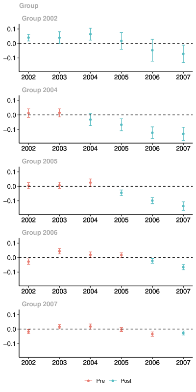
Figure 1: [29] estimates of group-time average treatment effects

Notes: The figure contains estimates of group-time average treatment effects for all available groups and time periods using the approach in [29] using the never-treated group as the comparison group and under unconditional parallel trends.

Next, the first set of overall treatment effect estimates are reported in Table 2. These results come from TWFE regressions using the five different datasets above. The results vary notably across different datasets with estimates ranging from minimum wage changes decreasing teen employment by 3.7% on average (relative to teen employment in the absence of the minimum wage change) to minimum wage changes increasing teen employment by 1.1% (which is marginally statistically significant). Interestingly, these estimates essentially run the gamut of estimates of minimum wage effects in the literature.

Table 2: TWFE estimates of overall effects

		Data 1	Data 2	Data 3	Data 4	Data 5
TWFE Est.
treated		$-0.037$*	$-0.035$*	$-0.026$*	$-0.009$	$0.011$
		($0.005$)	($0.006$)	($0.006$)	($0.007$)	($0.006$)
Bacon Decomp.
Earlier v. Later		0.861	0.952	0.474	0.745	0.250
Later v. Earlier		0.139	0.048	0.526	0.255	0.750
% Weight	$p_{g}$
$g=2002$	0.015	0.014	0.014	0.021	0.027	0.000
$g=2004$	0.094	0.168	0.170	0.234	0.286	0.000
$g=2005$	0.057	0.098	0.099	0.128	0.151	0.000
$g=2006$	0.227	0.301	0.302	0.331	0.355	0.386
$g=2007$	0.608	0.419	0.414	0.284	0.181	0.614
Num.Obs.		$18\,851$	$17\,437$	$8932$	$7518$	$3222$

Notes: The top panel of the table (“TWFE Est.”) contains estimates of the coefficient of a binary treatment indicator in a TWFE regression as in Equation 1. The middle panel (“Bacon Decomp.”) contains results from a Bacon decomposition. The rows labeled “Earlier v. Later” contain the fraction of weight that the TWFE regression puts on comparisons involving units that become treated relative to not-yet-treated units (which are the sort of comparisons justified by the parallel trends assumption). The rows labeled “Later v. Earlier” contain the fraction of weight that the TWFE regression puts on comparisons involving units that become treated relative to already-treated units (which are the sort of “bad comparisons” that show up in TWFE regressions). The bottom panel (“% Weight”) contains (i) in the column labeled “$p_{g}$”, the actual fraction of observations in each group among all units that become treated, and (ii) the fraction of weight on each group coming from the TWFE regression. The columns report estimates separately by which data was used.

There are several explanations for why the estimates change across specifications. First, the fraction of weight on “bad comparisons” varies tremendously across the data that is used. For Data 2 (that does not include already treated units), only about 5% of the weight in the TWFE regression goes to bad comparisons. Including already treated units (as in Data 1) increases the amount of weight on bad comparisons to 14%. Removing the never-treated group from the data (as in Data 3, 4, and 5) results in substantially more weight being put on bad comparisons (ranging from 26% to 75%) as well as notable changes in the estimated effect of the minimum wage.

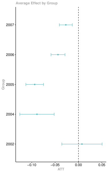
Figure 4: [29] group-specific average treatment effects

Another more subtle issue is that, even in the absence of the treatment effect dynamics (which would rationalize using already treated groups as comparison groups), the weights on underlying treatment effect parameters is still driven by the estimation method and varies across which data is used. To give an example, about 9% of counties that are ever treated become treated in 2004. However, the amount of total weight on the 2004 group of counties in the TWFE regression ranges from 0 to 29% across datasets. Further, there is notable variation in the effect of the treatment across groups (see, Figure 4 in Appendix B). This implies that variation in weights on group-time average treatment effects across regressions can cause changes in the TWFE estimates.

Table 3: Alternative estimates of overall effects

	TWFE	CS (NT)	CS (NYT)	CS (BTT)	Imp.	TWFE (D4)	CS (D4)	Imp (D4)
No Covariates	$-0.035^{*}$	$-0.040^{*}$	$-0.039^{*}$	$-0.033^{*}$	$-0.040^{*}$	$-0.009$	$-0.019^{*}$	$0.002$
	(0.006)	(0.005)	(0.005)	(0.005)	(0.008)	(0.007)	(0.007)	(0.009)
Covariates	$-0.020^{*}$	$-0.030^{*}$	$-0.028^{*}$		$-0.047^{*}$	$0.008$	$0.011$	$0.020^{*}$
	(0.006)	(0.005)	(0.006)		(0.006)	(0.007)	(0.009)	(0.009)

Notes: The table provides estimates of an overall ATT using different approaches discussed in the main text. The rows labeled “No Covariates” do not include any covariates; the rows labeled “Covariates” include the log of county population, the log of county average annual pay, and region fixed effects (with time varying coefficients). Columns labeled “TWFE” report estimates from a TWFE regression; columns labeled “CS (NT)”, “CS (NYT)”, and “CS (BTT)” report [29] estimates using the never-treated comparison group, the not-yet-treated comparison group, and the build-the-trend estimator discussed in the text, respectively; columns labeled “Imp.” report estimates from the imputation procedure discussed in the text. Estimates in the first five columns use Data 2; estimates in the last three columns use Data 4. CS and imputation estimates that include covariates drop states from the Northeast census region as all states eventually become treated in the Northeast which creates violations of underlying support assumptions for some time periods.

Finally, Table 3 provides treatment effect estimates using the new approaches discussed above. The first five columns provide estimates using Data 2. In the case where the researcher does not include additional covariates, the estimates are broadly similar to the TWFE estimates; however, it is still important to remember that none of the new approaches put any weight on “bad comparisons” and all of the weights are directly targeted at recovering the overall ATT. The second part of the table provides results when additional covariates are included; the additional covariates are the log of county population, the log of county average annual pay, and region (which is typically thought to be an important covariate in the minimum wage literature). There are larger differences between the TWFE results and new approaches in this case; for example, the TWFE estimate is about 30% smaller in magnitude than the CS estimates, and over 50% smaller than the imputation estimate. As discussed in Section 4.1, including covariates is the case with the biggest conceptual difference between CS and imputation — here, the CS approach effectively conditions on the pre-treatment level of the time varying covariates (and also enjoys the double robustness property) while the imputation approach effectively conditions on the change in the covariates over time in a linear model. The last three columns use Data 4 (which drops both always treated and never treated observations). These results are notably different. In this case, the CS estimates decrease in magnitude, and one of the imputation estimates is positive and statistically significant. The main explanation for this result is that the definition of “overall” average treatment effect changes in this case; in particular, when there is no available never-treated group, group-time average treatment effects are only identified up to 2006 (i.e., they are not available in 2007 anymore). However, notice that in Figure 1, the largest group-time average treatment effects tend to be in 2007. This suggests that, at least in the present context, changing the definition of overall ATT can lead to notably different estimates.

Event Study:

Next, Figure 2 compares the results from an event study regression using Data 1 and Data 2 to the the results using [29]. The results are fairly similar across methods/data though it is worth pointing out some interesting patterns. First, using Data 1, notice that the event study is estimated out until 6 periods after the treatment while it is only estimated out until 5 periods out using [29] and Data 2. At $e=6$, the event study regression estimates are essentially fully spurious and come from the group of counties already treated in 2001. This group also affects estimates at earlier lengths of exposure and explains the relatively large differences between the event study regressions using Data 1 and Data 2.

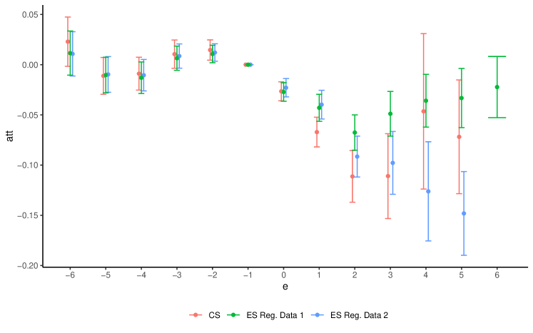
Figure 2: Event Study Comparison

Notes: The figure provides event study estimates of dynamic effects of participating in the treatment coming from using an event study regression with Data 2, and event study regression with Data 4, and an event study using the approach of [29].

Next, it is interesting to compare the results from [29] to the estimates from the event study regression using Data 2. The CS estimates are numerically equal to a weighted average of paths of outcomes from period $g-1$ to period $g+e$ among groups that participated in the treatment for $e$ periods relative to the path of outcomes of the never-treated group over the same time periods (and where the weights are given by the relative sizes of each available group). Take, for example, the estimate at $e=5$. There is only one group, $g=2002$, that is exposed to the treatment for 5 periods. The CS estimate is exactly equal to the average path of outcomes for $g=2002$ between 2001 and 2007 relative to the average path of outcomes for the never-treated group over the same periods. Exactly the same term shows up in $\beta_{5}$ in the event study regression with weight equal to 1 (which holds by additional property (ii) in Proposition 3). However, other terms also show up in the event study regression. For example, $ATT(g=2002,t=2002)$ gets a weight of -0.21 (which is the largest other weight in absolute value), and there are nine total group-time average treatment effects that get a weight of 0.1 or higher in absolute value (though it is undesirable that these have non-zero weight as they are all for event times other than $e=5$). Due to heterogeneous effects across groups and time periods, this moves the estimate from the event study regression away, at least to some extent, from the CS estimate; moreover, it is apparent that under a large amount of treatment effect heterogeneity, this event study regression could perform quite poorly.

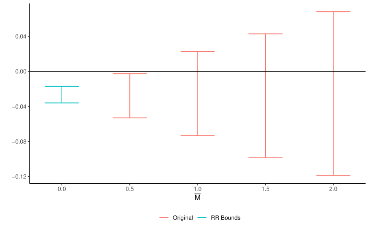
Figure 3: [66] Sensitivity Analysis

Notes: The figure provides a sensitivity analysis using the approach from [66] for the “on impact” ATT (i.e., for the CS event study in Figure 2 when $e=0$). The blue line contains the 95% confidence interval coming from the original estimate. The red lines provide 95% confidence sets allowing for violations of the parallel trends assumption up to $\bar{M}$ times as large as the maximum that occurred in pre-treatment periods.

Another thing that is interesting about the CS results in Figure 2 is that there appear to be some violations of parallel trends in pre-treatment periods (particularly, at $e=-2$, the point estimate is 0.015 and statistically different from 0). This suggests some limitations of the DID identification strategy. However, the “effects” in post-treatment periods are also statistically significant and seem large relative to the apparent violations of parallel trends. This sort of issue is likely to be fairly common in applications, and the sensitivity analysis discussed in Section 4.2 above is very well-suited for this setup. Results for the sensitivity analysis are reported in Figure 3 for $e=0$. The results indicate that the earlier conclusions are robust (in the sense of being statistically different from 0) to violations of parallel trends only up to half as large as were observed in pre-treatment periods. Allowing for violations of parallel trends as large as were observed in pre-treatment periods, the confidence set ranges from -0.073 to 0.023. This suggests a relatively wide range of possible effects of minimum wage increases on teen employment under violations of parallel trends similar to the ones that were observed in pre-treatment periods.

Discussion:

This section has considered several different approaches to estimating treatment effect parameters in a DID application with treatment effect heterogeneity and variation in treatment timing. There are several important takeaways from this application (and, arguably, these are generally representative of how using new approaches to DID can matter). First, as in any DID application, the most important concern is whether or not the parallel trends assumption actually holds. In this application, there is some evidence of moderately sized violations of the parallel trends assumption in pre-treatment periods. The [66] sensitivity analysis is particularly useful in this context and can be combined with any new DID approach. Second, treatment effect heterogeneity can matter a great deal. Under treatment effect heterogeneity, the definitions of target parameters can change due to data availability; for example, the results above were sensitive to whether or not treatment effects could be recovered in 2007 (where there tended to be the largest effects of participating in the treatment). Likewise, in the presence of treatment effect heterogeneity, the issue of having weights driven by the estimation method (as are the TWFE and event study regression weights) becomes more severe. Finally, in some cases there was a non-negligible amount of weight put on “bad comparisons” that use already treated units as the comparison group. The amount of weight on bad comparisons can be substantially mitigated by the researcher making good choices such as not including units that were already treated in the first period or by not including periods after all units have become treated. In general, the TWFE and event study regression estimates were not radically different from the estimates coming from new approaches; however, at least in some cases, there were differences that were large enough to suggest that researchers ought to use the new approaches.

6 Conclusion

Table 4: Further Reading on Related Topics

Additional Topic	References
More complicated treatment regimes (e.g., moving into and out of treatment, multi-valued or continuous treatments)	[42, 23]
Non-standard inference (e.g., small number of treated units or design-based inference)	[37, 44, 51, 8, 65]
Large-T panels (e.g., interactive fixed effects models, synthetic controls, matrix completion)	[2, 55, 49, 79, 5, 45, 6, 9]
Distributional effects (e.g., quantile treatment effects)	[7, 13, 36, 25, 27, 21]
Limited dependent variables (e.g., DID with a binary outcome)	[16, 77, 59]
Fuzzy DID (e.g., DID with aggregated data)	[40]
Sensitivity to functional form assumptions	[70]
Repeated cross sections and unbalanced panels	[1, 54, 15, 72]
DID surveys	[10, 33, 71]

This chapter has reviewed a number of recent, important advances in the econometrics literature on difference-in-differences. This literature has (i) pointed out a number of limitations of traditional regression-based approaches for implementing DID identification strategies in the presence of treatment effect heterogeneity, and (ii) proposed a set of alternative approaches that do not suffer from the same set of limitations. The new approaches are typically only slightly more complicated to implement, and there currently exist several well-developed software packages implementing the new approaches.

To conclude, there are a number of additional topics and extensions that this chapter did not cover. Table 4 lists some additional topics that may be of interest for particular applications where the goal is to study the causal effect of some economic policy/treatment and when a researcher has access to repeated observations over time. This is certainly an incomplete list but is meant to provide readers with a helpful springboard into related work.

Appendix A Proofs

Proof of Proposition 1

Proof.

To start with, well known Frisch-Waugh-Lovell type arguments imply that

$$\alpha=\frac{\displaystyle\frac{1}{\mathcal{T}}\sum_{t=1}^{\mathcal{T}}\mathbb{E}[\ddot{D}_{it}Y_{it}]}{\displaystyle\frac{1}{\mathcal{T}}\sum_{t=1}^{\mathcal{T}}\mathbb{E}[\ddot{D}_{it}^{2}]}$$

where, below (and unlike the main text), the notation sometimes indexes random variables by $i$ in places where it makes the arguments more clear. Next, notice that

$$\mathbb{E}[\ddot{D}_{it}]=0$$ (14)

Further, define $v(g,t)=\mathbf{1}\{t\geq g\}-\bar{G}_{g}$. Notice that, since treatment status is fully determined by group, one can re-write

$$D_{it}=\mathbf{1}\{t\geq G_{i}\},\hskip 20.0pt\bar{D}_{i}=\frac{1}{\mathcal{T}}\sum_{t=1}^{\mathcal{T}}D_{it}=\frac{\mathcal{T}-G_{i}+1}{\mathcal{T}},\hskip 20.0pt\mathbb{E}[D_{t}]=\textrm{P}(D_{t}=1)=\sum_{g\in\mathcal{G}}\mathbf{1}\{t\geq g\}p_{g}$$

and similarly that

$$\mathbb{E}[D_{t}]-\frac{1}{\mathcal{T}}\sum_{s=1}^{\mathcal{T}}\mathbb{E}[D_{s}] =\sum_{g\in\mathcal{G}}\mathbf{1}\{t\geq g\}p_{g}-\frac{1}{\mathcal{T}}\sum_{s=1}^{\mathcal{T}}\sum_{g\in\mathcal{G}}\mathbf{1}\{s\geq g\}p_{g}$$

$$=\sum_{g\in\mathcal{G}}\frac{1}{\mathcal{T}}\sum_{s=1}^{\mathcal{T}}\left(\mathbf{1}\{t\geq g\}-\mathbf{1}\{s\geq g\}\right)p_{g}$$

$$=\sum_{g\in\mathcal{G}}\left(\mathbf{1}\{t\geq g\}-\bar{G}_{g}\right)p_{g}$$

$$=\sum_{g\in\mathcal{G}}v(g,t)p_{g}$$

so that, in terms of $G_{i}$ and $t$,

$$\ddot{D}_{it} =\mathbf{1}\{t\geq G_{i}\}-\frac{\mathcal{T}-G_{i}+1}{\mathcal{T}}-\sum_{g\in\mathcal{G}}v(g,t)p_{g}$$

$$=v(G_{i},t)-\sum_{g\in\mathcal{G}}v(g,t)p_{g}$$ (15)

Now consider the numerator in the expression for $\alpha$

$$\frac{1}{\mathcal{T}}\sum_{t=1}^{\mathcal{T}}\mathbb{E}[\ddot{D}_{it}Y_{it}] =\frac{1}{\mathcal{T}}\sum_{t=1}^{\mathcal{T}}\mathbb{E}[\ddot{D}_{it}(Y_{it}-\mathbb{E}[Y_{t}])]$$

$$=\frac{1}{\mathcal{T}}\sum_{t=1}^{\mathcal{T}}\mathbb{E}[v(G_{i},t)(Y_{it}-\mathbb{E}[Y_{t}])]-\frac{1}{\mathcal{T}}\sum_{t=1}^{\mathcal{T}}\sum_{g\in\mathcal{G}}v(g,t)\,p_{g}\underbrace{\mathbb{E}\big{[}Y_{it}-\mathbb{E}[Y_{t}]\big{]}}_{=0}$$

$$=\frac{1}{\mathcal{T}}\sum_{t=1}^{\mathcal{T}}\sum_{g\in\mathcal{G}}v(g,t)(\mathbb{E}[Y_{t}|G=g]-\mathbb{E}[Y_{t}])\,p_{g}$$

$$=\frac{1}{\mathcal{T}}\sum_{t=1}^{\mathcal{T}}\sum_{g\in\mathcal{G}}v(g,t)\left(\mathbb{E}[Y_{t}|G=g]-\sum_{k\in\mathcal{G}}\mathbb{E}[Y_{t}|G=k]\,p_{k}\right)\,p_{g}$$

$$=\frac{1}{\mathcal{T}}\sum_{t=1}^{\mathcal{T}}\sum_{g\in\mathcal{G}}\sum_{k\in\mathcal{G}}v(g,t)\Big{(}\mathbb{E}[Y_{t}|G=g]-\mathbb{E}[Y_{t}|G=k]\Big{)}\,p_{k}\,p_{g}$$

$$=\frac{1}{\mathcal{T}}\sum_{t=1}^{\mathcal{T}}\sum_{g\in\mathcal{G}}\sum_{k\in\mathcal{G},k>g}(v(g,t)-v(k,t))\Big{(}\mathbb{E}[Y_{t}|G=g]-\mathbb{E}[Y_{t}|G=k]\Big{)}\,p_{k}\,p_{g}$$

where the first equality holds by Equation 14, the second equality holds by Equation 15, the third and fourth equalities hold by the law of iterated expectation, the fifth equality holds by re-arranging the summations, and the last equality holds because the summations are symmetric but with different “weights” $v(g,t)$.

Next, notice that

$$v(g,t)-v(k,t)=\begin{cases}\bar{G}_{k}-\bar{G}_{g}&\textrm{for }t<g<k\\ (1-\bar{G}_{g})+\bar{G}_{k}&\textrm{for }g\leq t<k\\ \bar{G}_{k}-\bar{G}_{g}&\textrm{for }g<k\leq t\end{cases}$$ (16)

Now, notice that

$$\frac{1}{\mathcal{T}}\sum_{t=1}^{\mathcal{T}}\sum_{g\in\mathcal{G}}\sum_{k\in\mathcal{G},k>g}(v(g,t)-v(k,t))\Big{(}\mathbb{E}[Y_{t}|G=g]-\mathbb{E}[Y_{t}|G=k]\Big{)}\,p_{k}\,p_{g}$$

$$\hskip 50.0pt=\sum_{g\in\mathcal{G}}\sum_{k\in\mathcal{G},k>g}\frac{1}{\mathcal{T}}\sum_{t=1}^{\mathcal{T}}(v(g,t)-v(k,t))\Big{(}\mathbb{E}[Y_{t}|G=g]-\mathbb{E}[Y_{t}|G=k]\Big{)}\,p_{k}\,p_{g}$$

$$\hskip 50.0pt=\sum_{g\in\mathcal{G}}\sum_{k\in\mathcal{G},k>g}\left\{\frac{1}{\mathcal{T}}\sum_{t=1}^{g-1}(v(g,t)-v(k,t))\Big{(}\mathbb{E}[Y_{t}|G=g]-\mathbb{E}[Y_{t}|G=k]\Big{)}\right.$$

$$\hskip 120.0pt+\left.\frac{1}{\mathcal{T}}\sum_{t=g}^{k-1}(v(g,t)-v(k,t))\Big{(}\mathbb{E}[Y_{t}|G=g]-\mathbb{E}[Y_{t}|G=k]\Big{)}\right.$$

$$\hskip 120.0pt+\left.\frac{1}{\mathcal{T}}\sum_{t=k}^{\mathcal{T}}(v(g,t)-v(k,t))\Big{(}\mathbb{E}[Y_{t}|G=g]-\mathbb{E}[Y_{t}|G=k]\Big{)}\right\}\,p_{k}\,p_{g}$$

$$\hskip 50.0pt=\sum_{g\in\mathcal{G}}\sum_{k\in\mathcal{G},k>g}\left\{\frac{g-1}{\mathcal{T}}(\bar{G}_{k}-\bar{G}_{g})\Big{(}\mathbb{E}[\bar{Y}^{PRE(g)}|G=g]-\mathbb{E}[\bar{Y}^{PRE(g)}|G=k]\Big{)}\right.$$

$$\hskip 120.0pt+\left.\frac{k-g}{\mathcal{T}}((1-\bar{G}_{g})+\bar{G}_{k})\Big{(}\mathbb{E}[\bar{Y}^{MID(g,k)}|G=g]-\mathbb{E}[\bar{Y}^{MID(g,k)}|G=k]\Big{)}\right.$$

$$\hskip 120.0pt+\left.\frac{\mathcal{T}-k+1}{\mathcal{T}}(\bar{G}_{k}-\bar{G}_{g})\Big{(}\mathbb{E}[\bar{Y}^{POST(k)}|G=g]-\mathbb{E}[\bar{Y}^{POST(k)}|G=k]\Big{)}\right\}\,p_{k}\,p_{g}$$

$$\hskip 50.0pt=\sum_{g\in\mathcal{G}}\sum_{k\in\mathcal{G},k>g}\left\{(1-\bar{G}_{g})(\bar{G}_{k}-\bar{G}_{g})\Big{(}\mathbb{E}[\bar{Y}^{PRE(g)}|G=g]-\mathbb{E}[\bar{Y}^{PRE(g)}|G=k]\Big{)}\right.$$

$$\hskip 120.0pt+\left.(\bar{G}_{g}-\bar{G}_{k})((1-\bar{G}_{g})+\bar{G}_{k})\Big{(}\mathbb{E}[\bar{Y}^{MID(g,k)}|G=g]-\mathbb{E}[\bar{Y}^{MID(g,k)}|G=k]\Big{)}\right.$$

$$\hskip 120.0pt+\left.\bar{G}_{k}(\bar{G}_{k}-\bar{G}_{g})\Big{(}\mathbb{E}[\bar{Y}^{POST(k)}|G=g]-\mathbb{E}[\bar{Y}^{POST(k)}|G=k]\Big{)}\right\}\,p_{k}\,p_{g}$$

$$\hskip 50.0pt=\sum_{g\in\mathcal{G}}\sum_{k\in\mathcal{G},k>g}\left\{(1-\bar{G}_{g})(\bar{G}_{g}-\bar{G}_{k})\Big{(}\mathbb{E}[\bar{Y}^{MID(g,k)}-\bar{Y}^{PRE(g)}|G=g]-\mathbb{E}[\bar{Y}^{MID(g,k)}-\bar{Y}^{PRE(g)}|G=k]\Big{)}\right.$$

$$\hskip 120.0pt+\left.\bar{G}_{k}(\bar{G}_{g}-\bar{G}_{k})\Big{(}\mathbb{E}[\bar{Y}^{POST(k)}-\bar{Y}^{MID(g,k)}|G=k]-\mathbb{E}[\bar{Y}^{POST(k)}-\bar{Y}^{MID(g,k)}|G=g]\Big{)}\right\}\,p_{k}\,p_{g}$$

where the first equality changes the order of the summations, the second equality splits the summations by “PRE”, “MID”, and “POST” periods, the third equality holds from Equation 16 and by the definitions of $\bar{Y}^{PRE(g)}$, $\bar{Y}^{MID(g,k)}$, and $\bar{Y}^{POST(k)}$, the fourth equality holds by the definition of $\bar{G}_{g}$, and the last equality holds by rearranging and combining terms. Finally, notice that $p_{g}=p_{g|\{g,k\}}(p_{g}+p_{k})$; plugging this expression in and the analogous expression for $p_{k}$ completes the proof. ∎

Proof of Proposition 2

Proof.

$$ATT(g,t) =\mathbb{E}[Y_{t}(g)-Y_{t}(0)|G=g]$$

$$=\mathbb{E}[Y_{t}(g)-Y_{g-1}(0)|G=g]-\mathbb{E}[Y_{t}(0)-Y_{g-1}(0)|G=g]$$

$$=\mathbb{E}[Y_{t}(g)-Y_{g-1}(0)|G=g]-\sum_{s=g}^{t}\mathbb{E}[Y_{s}(0)-Y_{s-1}(0)|G=g]$$

$$=\mathbb{E}[Y_{t}(g)-Y_{g-1}(0)|G=g]-\sum_{s=g}^{t}\mathbb{E}[Y_{s}(0)-Y_{s-1}(0)|G=\mathcal{T}+1]$$

$$=\mathbb{E}[Y_{t}(g)-Y_{g-1}(0)|G=g]-\mathbb{E}[Y_{t}(0)-Y_{g-1}(0)|G=\mathcal{T}+1]$$

$$=\mathbb{E}[Y_{t}-Y_{g-1}|G=g]-\mathbb{E}[Y_{t}-Y_{g-1}|G=\mathcal{T}+1]$$

where the first equality holds from the definition of $ATT(g,t)$, the second equality holds by adding and subtracting $\mathbb{E}[Y_{g-1}(0)|G=g]$, the third equality holds by adding and subtracting $\mathbb{E}[Y_{s}(0)|G=g]$ for all $s=g,\ldots,t-1$, the fourth equality holds by Assumption 4, the fifth equality cancels all the terms involving $\mathbb{E}[Y_{s}(0)|G=\mathcal{T}+1]$ for $s=g,\ldots,t-1$, and the last equality re-writes potential outcomes in terms of their observed counterparts. ∎

Proof of Proposition 3

Proof.

To start with, notice that the event study regression in Equation 9 can be re-written as

$$Y_{it}=\theta_{t}+\eta_{i}+\mathbf{D}_{it}^{\prime}\beta+v_{it}$$

where $\beta$ is the $2(\mathcal{T}-1)$ dimensional vector that collects all of the $\beta_{e}$ in Equation 9. Standard Frisch-Waugh types of arguments then imply that

$$\beta_{e} =\mathbf{e}_{e}^{\prime}\left(\sum_{t=1}^{\mathcal{T}}\mathbb{E}[\ddot{\mathbf{D}}_{it}\ddot{\mathbf{D}}_{it}^{\prime}]\right)^{-1}\sum_{t=1}^{\mathcal{T}}\mathbb{E}[\ddot{\mathbf{D}}_{it}Y_{it}]$$ (17)

where, with a slight abuse of notation, $\mathbf{e}_{e}$ is the $2(\mathcal{T}-1)$ column vector with 1 in the position corresponding to $e$ and all other elements equal to 0.

The results below use the following properties of double-demeaned variables: (i) $\mathbb{E}[\ddot{\mathbf{D}}_{it}]=0$; (ii) for some random variable, $Z_{i}$, that does not depend on the time period $\sum_{t=1}^{\mathcal{T}}\mathbb{E}[\ddot{\mathbf{D}}_{it}Z_{i}]=0$; and (iii) $\mathbb{E}[\ddot{\mathbf{D}}_{it}\ddot{\mathbf{D}}_{it}^{\prime}]=\mathbb{E}[\ddot{\mathbf{D}}_{it}\mathbf{D}_{it}^{\prime}]$. These are all well-known properties of double-demeaning (see, for example, [76]). Property (ii) implies that

$$\sum_{t=1}^{\mathcal{T}}\mathbb{E}[\ddot{\mathbf{D}}_{it}Y_{iG_{i}-1}]=0$$ (18)

and property (i) implies that

$$\mathbb{E}[\ddot{\mathbf{D}}_{it}]\sum_{g\in\mathcal{G}}\mathbb{E}[Y_{it}-Y_{ig-1}|G=\mathcal{T}+1]p_{g}=0$$ (19)

Further, recall that a typical element of $\mathbf{D}_{it}$ is given by $D_{it}^{e}=\mathbf{1}\{t-G_{i}=e\}\mathbf{1}\{G_{i}<\mathcal{T}+1\}$. This implies that

$$\bar{D}_{i}^{e} =\frac{1}{\mathcal{T}}\sum_{t=1}^{\mathcal{T}}\mathbf{1}\{t-G_{i}=e\}\mathbf{1}\{G_{i}<\mathcal{T}+1\}$$

$$=\frac{\mathbf{1}\{(G_{i}+e)\in[1,\mathcal{T}]\}}{\mathcal{T}}\mathbf{1}\{G_{i}<\mathcal{T}+1\}$$

where the second equality holds because $t$ can, at most, equal $G_{i}+e$ for only one value of $t=1,\ldots,\mathcal{T}$, and that

$$\mathbb{E}[D_{t}^{e}]=\sum_{g\in\mathcal{G}}\mathbf{1}\{t-g=e\}\mathbf{1}\{g<\mathcal{T}+1\}\,p_{g}$$

and

$$\frac{1}{\mathcal{T}}\sum_{s=1}^{\mathcal{T}}\mathbb{E}[D_{s}^{e}] =\frac{1}{\mathcal{T}}\sum_{s=1}^{\mathcal{T}}\sum_{g\in\mathcal{G}}\mathbf{1}\{t=g+e\}\mathbf{1}\{g<\mathcal{T}+1\}\,p_{g}$$

$$=\sum_{g\in\mathcal{G}}\frac{\mathbf{1}\{g+e\in[1,\mathcal{T}]\}}{\mathcal{T}}\mathbf{1}\{g<\mathcal{T}+1\}\,p_{g}$$

Next, recall that $\tilde{h}_{e}(g,t)=\Big{(}\mathbf{1}\{t-g=e\}-\frac{\mathbf{1}\{(g+e)\in[1,\mathcal{T}]\}}{\mathcal{T}}\Big{)}\mathbf{1}\{g<\mathcal{T}+1\}$. Thus, a typical element of $\ddot{\mathbf{D}}_{it}$ is given by

$$\ddot{D}_{it}^{e}=\tilde{h}_{e}(G_{i},t)-\sum_{g\in\mathcal{G}}\tilde{h}_{e}(g,t)\,p_{g}$$ (20)

and that $\ddot{\mathbf{D}}_{it}=h(G_{i},t)$ where $h(g,t)$ is a $2(\mathcal{T}-1)$ vector with typical element given by $\tilde{h}_{e}(g,t)-\sum_{k\in\mathcal{G}}\tilde{h}_{e}(k,t)\,p_{k}$

There are several properties of $h(g,t)$ that are used below. First, for any $g$ and $e$,

$$\sum_{t=1}^{\mathcal{T}}\tilde{h}_{e}(g,t) =\sum_{t=1}^{\mathcal{T}}\left(\mathbf{1}\{t-g=e\}-\frac{\mathbf{1}\{(g+e)\in[1,\mathcal{T}]\}}{\mathcal{T}}\right)\mathbf{1}\{g<\mathcal{T}+1\}$$

$$=\mathbf{1}\{g<\mathcal{T}+1\}\left(\mathbf{1}\{(g+e)\in[1,\mathcal{T}]\}-\sum_{t=1}^{\mathcal{T}}\frac{\mathbf{1}\{(g+e)\in[1,\mathcal{T}]\}}{\mathcal{T}}\right)$$

$$=0$$

which immediately implies that

$$\sum_{t=1}^{\mathcal{T}}h(g,t)=0$$ (21)

Another useful property is that

$$\sum_{t=1}^{\mathcal{T}}\sum_{g\in\mathcal{G}}h(g,t)\mathbb{E}[Y_{t}|G=\mathcal{T}+1]p_{g} =\sum_{t=1}^{\mathcal{T}}\mathbb{E}[Y_{t}|G=\mathcal{T}+1]\sum_{g\in\mathcal{G}}h(g,t)p_{g}$$

$$=\sum_{t=1}^{\mathcal{T}}\mathbb{E}[Y_{t}|G=\mathcal{T}+1]\mathbb{E}[h(G_{i},t)]$$

$$=\sum_{t=1}^{\mathcal{T}}\mathbb{E}[Y_{t}|G=\mathcal{T}+1]\mathbb{E}[\ddot{\mathbf{D}}_{it}]$$

$$=0$$ (22)

where the third equality holds by the definition of $h(G_{i},t)$, and the last equality holds because $\mathbb{E}[\ddot{\mathbf{D}}_{it}]=0$. Additionally, notice that

$$\sum_{t=1}^{\mathcal{T}}\sum_{g\in\mathcal{G}}h(g,t)\mathbb{E}[Y_{g-1}|G=\mathcal{T}+1]p_{g} =\sum_{g\in\mathcal{G}}\mathbb{E}[Y_{g-1}|G=\mathcal{T}+1]p_{g}\sum_{t=1}^{\mathcal{T}}h(g,t)$$

$$=0$$ (23)

where the last equality holds because $\sum_{t=1}^{\mathcal{T}}h(g,t)=0$. Therefore, it follows from Equations 22 and 23 that

$$\sum_{t=1}^{\mathcal{T}}\sum_{g\in\mathcal{G}}h(g,t)\mathbb{E}[Y_{it}-Y_{ig-1}|G=\mathcal{T}+1]p_{g} =\sum_{t=1}^{\mathcal{T}}\sum_{g\in\mathcal{G}}h(g,t)\mathbb{E}[Y_{t}|G=\mathcal{T}+1]p_{g}-\sum_{t=1}^{\mathcal{T}}\sum_{g\in\mathcal{G}}h(g,t)\mathbb{E}[Y_{g-1}|G=\mathcal{T}+1]p_{g}$$

$$=0$$ (24)

Now, consider the “numerator” in Equation 17.

$$\sum_{t=1}^{\mathcal{T}}\mathbb{E}[\ddot{\mathbf{D}}_{it}Y_{it}] =\sum_{t=1}^{\mathcal{T}}\mathbb{E}[\ddot{\mathbf{D}}_{it}Y_{it}]-\sum_{t=1}^{\mathcal{T}}\mathbb{E}[\ddot{\mathbf{D}}_{it}Y_{iG_{i}-1}]$$

$$=\sum_{t=1}^{\mathcal{T}}\mathbb{E}[h(G_{i},t)(Y_{it}-Y_{iG_{i}-1})]$$

$$=\sum_{t=1}^{\mathcal{T}}\sum_{g\in\mathcal{G}}h(g,t)\mathbb{E}[Y_{it}-Y_{ig-1}|G_{i}=g]\,p_{g}$$

$$=\sum_{t=1}^{\mathcal{T}}\sum_{g\in\mathcal{G}}h(g,t)\mathbb{E}[Y_{it}-Y_{ig-1}|G_{i}=g]\,p_{g}-\sum_{t=1}^{\mathcal{T}}\sum_{g\in\mathcal{G}}h(g,t)\mathbb{E}[Y_{it}-Y_{ig-1}|G=\mathcal{T}+1]p_{g}$$

$$=\sum_{t=1}^{\mathcal{T}}\sum_{g\in\mathcal{G}}h(g,t)\big{(}\mathbb{E}[Y_{it}-Y_{ig-1}|G_{i}=g]-\mathbb{E}[Y_{it}-Y_{ig-1}|G=\mathcal{T}+1]\big{)}\,p_{g}$$

$$=\sum_{t=1}^{\mathcal{T}}\sum_{g\in\mathcal{G}}h(g,t)\sum_{l=-(\mathcal{T}-1)}^{\mathcal{T}-1}\big{(}\mathbb{E}[Y_{ig+l}-Y_{ig-1}|G_{i}=g]-\mathbb{E}[Y_{ig+l}-Y_{ig-1}|G=\mathcal{T}+1]\big{)}\mathbf{1}\{g+l=t\}\mathbf{1}\{g<\mathcal{T}+1\}\,p_{g}$$

$$=\sum_{l=-(\mathcal{T}-1)}^{\mathcal{T}-1}\sum_{g\in\bar{\mathcal{G}}}h(g,g+l)\,p_{g}\big{(}\mathbb{E}[Y_{ig+l}-Y_{ig-1}|G_{i}=g]-\mathbb{E}[Y_{ig+l}-Y_{ig-1}|G=\mathcal{T}+1]\big{)}\underbrace{\sum_{t=1}^{\mathcal{T}}\mathbf{1}\{g+l=t\}}_{=\mathbf{1}\{g+l\in[1,T]\}}$$

where the first equality holds by Equation 18, the second equality holds by the definition of $h(G_{i},t)$, the third equality holds by the law of iterated expectations, the fourth equality holds by Equation 24, the fifth equality holds by combining terms, the sixth equality holds because the indicator inside the new summation only picks up the original term (and the inside term is equal to 0 when $g=\mathcal{T}+1$), and the last equality holds by rearranging summations and by summing over only groups that are ever treated (i.e., where $g<\mathcal{T}+1$).

This implies that

$$\beta_{e}=\sum_{l=-(\mathcal{T}-1)}^{\mathcal{T}+1}\sum_{g\in\bar{\mathcal{G}}}w^{ES}_{e}(g,l)\big{(}\mathbb{E}[Y_{ig+l}-Y_{g-1}|G=g]-\mathbb{E}[Y_{ig+l}-Y_{ig-1}|G=\mathcal{T}+1]\big{)}$$

where

$$w^{ES}_{e}(g,l)=\mathbf{e}_{e}^{\prime}\left(\sum_{t=1}^{\mathcal{T}}\mathbb{E}[\ddot{\mathbf{D}}_{it}\ddot{\mathbf{D}}_{it}^{\prime}]\right)^{-1}h(g,g+l)\mathbf{1}\{g+l\in[1,\mathcal{T}]\}\,p_{g}$$

This completes the first part of the proof. The next part shows the additional properties of the weights provided in the proposition. Towards this end, notice that

$$\sum_{g\in\bar{\mathcal{G}}}h(g,g+l)\mathbf{1}\{g+l\in[1,\mathcal{T}]\}\,p_{g} =\sum_{g\in\bar{\mathcal{G}}}\sum_{t=1}^{\mathcal{T}}h(g,t)\mathbf{1}\{t=g+l\}\,p_{g}$$

$$=\sum_{t=1}^{\mathcal{T}}\sum_{g\in\mathcal{G}}h(g,t)\mathbf{1}\{t=g+l\}\mathbf{1}\{g<\mathcal{T}+1\}\,p_{g}$$

$$=\sum_{t=1}^{\mathcal{T}}\mathbb{E}\left[h(G_{i},t)\mathbf{1}\{t=G_{i}+l\}\mathbf{1}\{G_{i}<\mathcal{T}+1\}\right]$$

$$=\sum_{t=1}^{\mathcal{T}}\mathbb{E}[\ddot{\mathbf{D}}_{it}D_{it}^{l}]$$

$$=\sum_{t=1}^{\mathcal{T}}\mathbb{E}[\ddot{\mathbf{D}}_{it}\ddot{D}_{it}^{l}]$$ (25)

where the first equality holds because $\mathbf{1}\{t=g+l\}$ holds at most once from $t=1,\ldots,\mathcal{T}$, the second equality changes the order of summations and sums across all groups, the third equality holds by the definition of expectation, the fourth equality holds by the definitions of $h(G,t)$ and $D_{it}^{l}$, and the last equality holds by the properties of double de-meaned random variables. Thus,

$$\sum_{g\in\bar{\mathcal{G}}}\left(\sum_{t=1}^{\mathcal{T}}\mathbb{E}[\ddot{\mathbf{D}}_{it}\ddot{\mathbf{D}}_{it}^{\prime}]\right)^{-1}h(g,g+l)\mathbf{1}\{g+l\in[1,\mathcal{T}]\}\,p_{g} =\left(\sum_{t=1}^{\mathcal{T}}\mathbb{E}[\ddot{\mathbf{D}}_{it}\ddot{\mathbf{D}}_{it}^{\prime}]\right)^{-1}\sum_{t=1}^{\mathcal{T}}\mathbb{E}[\ddot{\mathbf{D}}_{it}\ddot{D}_{it}^{l}]$$

$$=\mathbf{e}_{l}$$

where the first equality holds by Appendix A, and the last equality holds because the previous line amounts to a regression of $\ddot{D}_{it}^{l}$ on $\ddot{\mathbf{D}}_{it}$ (of with $\ddot{D}_{it}^{l}$ is an element and, therefore, the coefficients from this regression are all equal to 0 except the one on $\ddot{D}_{it}^{l}$ which is equal to 1). This further implies that,

$$\sum_{g\in\bar{\mathcal{G}}}w_{e}^{ES}(g,l)=\mathbf{e}_{e}^{\prime}\mathbf{e}_{l}$$

which is equal to 1 when $l=e$ and equal to 0 when $l\neq e$. This implies the additional properties of the weights. ∎

Proof of Proposition 4

Proof.

Start by rewriting the expression for $ATT(g,t)$ as

$$ATT(g,t) =\mathbb{E}\left[\frac{\mathbf{1}\{G=g\}}{p_{g}}\big{(}Y_{t}-Y_{g-1}-m^{nt}_{gt}(X)\big{)}\right]-\mathbb{E}\left[\frac{\frac{p_{g}(X)U}{p_{g}(1-p_{g}(X))}}{\mathbb{E}\left[\frac{p_{g}(X)U}{p_{g}(1-p_{g}(X))}\right]}\big{(}Y_{t}-Y_{g-1}-m^{nt}_{gt}(X)\big{)}\right]$$

$$:=A-B$$

For Term A, notice that

$$A =\mathbb{E}\left[Y_{t}-Y_{g-1}|G=g\right]-\mathbb{E}\left[\mathbb{E}[Y_{t}-Y_{g-1}|X,U=1]\Big{|}G=g\right]$$

$$=\mathbb{E}\left[Y_{t}(1)-Y_{g-1}(0)|G=g\right]-\mathbb{E}\left[\mathbb{E}[Y_{t}(0)-Y_{g-1}(0)|X,U=1\Big{|}G=g\right]$$

$$=\mathbb{E}\left[Y_{t}(1)-Y_{g-1}(0)|G=g\right]-\mathbb{E}\left[\mathbb{E}[Y_{t}(0)-Y_{g-1}(0)|X,G=g\Big{|}G=g\right]$$

$$=\mathbb{E}\left[Y_{t}(1)-Y_{g-1}(0)|G=g\right]-\mathbb{E}\left[Y_{t}(0)-Y_{g-1}(0)|G=g\right]$$

$$=\mathbb{E}\left[Y_{t}(1)-Y_{t}(0)|G=g\right]$$

$$=ATT(g,t)$$

where the first equality holds by the law of iterated expectations and by the definition of $m_{gt}^{nt}(X)$, the second equality holds by writing observed outcomes in terms of their corresponding potential outcomes, the third equality holds by Assumption 5, the fourth equality holds by the law of iterated expectations, the sixth equality cancels $\mathbb{E}[Y_{g-1}(0)|G=g]$ from each term, and the last equality holds by the definition of $ATT(g,t)$.

For term B, first notice for the denominator in the “weights” that

$$\mathbb{E}\left[\frac{p_{g}(X)U}{p_{g}(1-p_{g}(X))}\right] =\mathbb{E}\left[\frac{p_{g}(X)U}{p_{g}(1-p_{g}(X))}\Big{|}\mathbf{1}\{G=g\}+U=1\right]\,(p_{g}+p_{U})$$

$$=\mathbb{E}\left[\frac{p_{g}(X)}{p_{g}(1-p_{g}(X))}\mathbb{E}[U|X,\mathbf{1}\{G=g\}+U=1]\Big{|}\mathbf{1}\{G=g\}+U=1\right](p_{g}+p_{U})$$

$$=\frac{\mathbb{E}[p_{g}(X)|\mathbf{1}\{G=g\}+U=1]}{p_{g}}(p_{g}+p_{U})$$

$$=\frac{p_{g|\{g,U\}}}{p_{g}}{(p_{g}+p_{U})}$$

$$=1$$ (26)

where the first and second equalities hold by the law of iterated expectations, the third equality holds because $\mathbb{E}[U|X,\mathbf{1}\{G=g\}+U=1]=1-p_{g}(X)$, the fourth equality holds by the definition of $p_{g}(X)$ and the law of iterated expectations, and the last equality because $p_{g|\{g,U\}}=p_{g}/(p_{g}+p_{U})$. Thus,

$$B =\mathbb{E}\left[\frac{p_{g}(X)U}{p_{g}(1-p_{g}(X))}\Big{(}(Y_{t}-Y_{g-1})-\mathbb{E}[Y_{t}-Y_{g-1}|X,U=1]\Big{)}\right]$$

$$=\mathbb{E}\left[\frac{p_{g}(X)}{p_{g}(1-p_{g}(X))}\Big{(}(Y_{t}-Y_{g-1})-\mathbb{E}[Y_{t}-Y_{g-1}|X,U=1]\Big{)}\Big{|}U=1\right]p_{U}$$

$$=\mathbb{E}\left[\frac{p_{g}(X)}{p_{g}(1-p_{g}(X))}\underbrace{\Big{(}\mathbb{E}[Y_{t}-Y_{g-1}|X,U=1]-\mathbb{E}[Y_{t}-Y_{g-1}|X,U=1]\Big{)}}_{=0}\Big{|}U=1\right]p_{U}$$

$$=0$$

where the first equality holds by Equation 26, and the second and third equalities hold by the law of iterated expectations. This implies the first part of the result.

To show the double robustness property, let $p_{g}(X;\pi)$ denote a parametric working model for $p_{g}(X)$ and $m_{gt}^{nt}(X,\beta)$ denote a parametric working model for $m_{gt}^{nt}(X)$; let $\pi^{*}$ and $\beta^{*}$ denote the pseudo-true values of the parameters. First, consider the case where $m_{gt}^{nt}(X,\beta^{*})=m_{gt}^{nt}(X)$ so that the outcome regression model is correctly specified but allow for the possibility that the propensity score model is not correctly specified. In this case, the arguments are analogous to above: the arguments for term A did not rely on the propensity score model, and the arguments for term B also go through with $p_{g}(X,\pi^{*})$ replacing $p_{g}(X)$ and without requiring this model to be correctly specified (given that $m_{gt}^{nt}(X,\beta^{*})$ is correctly specified).

Finally, consider the case where the propensity score model is correctly specified, but the outcome regression may not be correctly specified. In this case,

$$A =\mathbb{E}[Y_{t}(1)-Y_{g-1}(0)|G=g]-\mathbb{E}[m_{gt}^{nt}(X;\beta^{*})|G=g]$$

and

$$B =\mathbb{E}\left[\frac{p_{g}(X)U}{p_{g}(1-p_{g}(X))}\Big{(}(Y_{t}-Y_{g-1})-m_{gt}^{nt}(X;\beta^{*})\Big{)}\right]$$

$$:=B_{1}-B_{2}$$

Next,

$$B_{1} =\mathbb{E}\left[\frac{p_{g}(X)U}{p_{g}(1-p_{g}(X))}(Y_{t}-Y_{g-1})\right]$$

$$=\mathbb{E}\left[\frac{p_{g}(X)}{p_{g}(1-p_{g}(X))}\big{(}Y_{t}(0)-Y_{g-1}(0)\big{)}\Big{|}U=1\right]p_{U}$$

$$=\mathbb{E}\left[\frac{p_{g}(X)}{p_{g}(1-p_{g}(X))}\mathbb{E}[Y_{t}(0)-Y_{g-1}(0)|X,U=1]\Big{|}U=1\right]p_{U}$$

$$=\mathbb{E}\left[\mathbb{E}[Y_{t}(0)-Y_{g-1}(0)|X,U=1]\Big{|}G=g\right]$$

$$=\mathbb{E}\left[\mathbb{E}[Y_{t}(0)-Y_{g-1}(0)|X,G=g]\Big{|}G=g\right]$$

$$=\mathbb{E}\left[Y_{t}(0)-Y_{g-1}(0)|G=g\right]$$

where the second equality holds by the law of iterated expectations and writing observed outcomes in terms of their corresponding potential outcomes, the third equality holds by the law of iterated expectations, the fourth equality holds by integrating with respect to group $g$ rather than the untreated group and re-weighting, the fifth equality holds by Assumption 5, and the last equality holds by the law of iterated expectations. Finally,

$$B_{2} =\mathbb{E}\left[\frac{p_{g}(X)}{p_{g}(1-p_{g}(X))}m_{gt}^{nt}(X;\beta^{*})\Big{)}\Big{|}U=1\right]p_{U}$$

$$=\mathbb{E}\left[m_{gt}^{nt}(X;\beta^{*})\Big{|}G=g\right]$$

This implies that, in this case, $A-B=ATT(g,t)$ which implies the double robustness property. ∎

A.1 Explanation for Build-the-Trend Estimator

This section provides the corresponding estimand for $\widehat{ATT}^{CS}_{\textrm{build-the-trend}}(g,t)$ stated as a proposition.

Proposition 5.

In the setup considered in Section 3 and under Assumptions 3 and 4, $g\in\bar{\mathcal{G}}$, and for all $t\geq g$ (i.e., post-treatment time periods for group $g$),

$$ATT(g,t)=\mathbb{E}[Y_{t}(g)-\bar{Y}^{PRE(g)}|G=g]-\sum_{l=2}^{t}\tilde{w}_{btt}(g,l)\mathbb{E}[Y_{l}-Y_{l-1}|D_{l}=0,G\neq g]$$

where $\tilde{w}_{btt}(g,l)=\min\left(1,\frac{l-1}{g-1}\right)$.

Proof.

$$ATT(g,t) =\mathbb{E}[Y_{t}(g)-Y_{t}(0)|G=g]$$

$$=\frac{1}{g-1}\sum_{s=1}^{g-1}\mathbb{E}[Y_{t}(g)-Y_{s}(0)|G=g]-\frac{1}{g-1}\sum_{s=1}^{g-1}\mathbb{E}[Y_{t}(0)-Y_{s}(0)|G=g]$$

$$=\mathbb{E}[Y_{t}-\bar{Y}^{PRE(g)}|G=g]-\frac{1}{g-1}\sum_{s=1}^{g-1}\sum_{l=s+1}^{t}\mathbb{E}[Y_{l}(0)-Y_{l-1}(0)|G=g]$$

$$=\mathbb{E}[Y_{t}-\bar{Y}^{PRE(g)}|G=g]-\frac{1}{g-1}\sum_{s=1}^{g-1}\sum_{l=2}^{t}\mathbf{1}\{l\geq s+1\}\mathbb{E}[Y_{l}(0)-Y_{l-1}(0)|G=g]$$

$$=\mathbb{E}[Y_{t}-\bar{Y}^{PRE(g)}|G=g]-\sum_{l=2}^{t}\mathbb{E}[Y_{l}(0)-Y_{l-1}(0)|G=g]\frac{1}{g-1}\sum_{s=1}^{g-1}\mathbf{1}\{s\leq l-1\}$$

$$=\mathbb{E}[Y_{t}-\bar{Y}^{PRE(g)}|G=g]-\sum_{l=2}^{t}\tilde{w}_{btt}(g,l)\mathbb{E}[Y_{l}(0)-Y_{l-1}(0)|G=g]$$

$$=\mathbb{E}[Y_{t}-\bar{Y}^{PRE(g)}|G=g]-\sum_{l=2}^{t}\tilde{w}_{btt}(g,l)\mathbb{E}[Y_{l}(0)-Y_{l-1}(0)|D_{l}=0,G\neq g]$$

where the first equality uses the definition of $ATT(g,t)$, the second equality amounts to using all pre-treatment periods as the “base period” and averaging over these, the third equality holds by replacing potential outcomes with their observed counterparts and because all the intermediate terms in the second part cancel with each other, the fourth equality changes the limits of the inside summation, the fifth equality holds by changing the order of the summation and then rearranging terms, the sixth equality holds by the definition of $\tilde{w}_{btt}$, and the last equality holds under Assumption 4. ∎

Appendix B Additional Figures

Notes: The figure contains estimates of group-specific average treatment effects (average across all available post-treatment time periods for a particular group) for all available groups using the approach in [29] using the never-treated group as the comparison group and under unconditional parallel trends.

References

- [1] Alberto Abadie “Semiparametric difference-in-differences estimators” In The Review of Economic Studies 72.1 Oxford University Press, 2005, pp. 1–19
- [2] Alberto Abadie, Alexis Diamond and Jens Hainmueller “Synthetic control methods for comparative case studies: Estimating the effect of California’s tobacco control program” In Journal of the American Statistical Association 105.490 Taylor & Francis, 2010, pp. 493–505
- [3] Joshua D Angrist and Jorn-Steffen Pischke “Mostly Harmless Econometrics: An Empiricist’s Companion” Princeton University Press, 2008
- [4] Vincent Arel-Bundock “modelsummary: Summary Tables and Plots for Statistical Models and Data: Beautiful, Customizable, and Publication-Ready” R package version 0.9.6, 2022 URL: https://CRAN.R-project.org/package=modelsummary
- [5] Dmitry Arkhangelsky, Susan Athey, David A Hirshberg, Guido W Imbens and Stefan Wager “Synthetic difference-in-differences” In American Economic Review 111.12, 2021, pp. 4088–4118
- [6] Susan Athey, Mohsen Bayati, Nikolay Doudchenko, Guido Imbens and Khashayar Khosravi “Matrix completion methods for causal panel data models” In Journal of the American Statistical Association Taylor & Francis, 2021, pp. 1–15
- [7] Susan Athey and Guido Imbens “Identification and inference in nonlinear difference-in-differences models” In Econometrica 74.2 Wiley Online Library, 2006, pp. 431–497
- [8] Susan Athey and Guido W Imbens “Design-based analysis in difference-in-differences settings with staggered adoption” In Journal of Econometrics 226.1 Elsevier, 2022, pp. 62–79
- [9] Jushan Bai and Serena Ng “Matrix completion, counterfactuals, and factor analysis of missing data” In Journal of the American Statistical Association Taylor & Francis, 2021
- [10] Andrew Baker, David F Larcker and Charles CY Wang “How much should we trust staggered difference-in-differences estimates?” forthcoming at Journal of Financial Economics, 2021
- [11] Laurent Bergé “Efficient estimation of maximum likelihood models with multiple fixed-effects: the R package FENmlm” In CREA Discussion Papers, 2018
- [12] Richard Blundell and Monica Costa Dias “Alternative approaches to evaluation in empirical microeconomics” In Journal of Human Resources 44.3 University of Wisconsin Press, 2009, pp. 565–640
- [13] Stephane Bonhomme and Ulrich Sauder “Recovering distributions in difference-in-differences models: A comparison of selective and comprehensive schooling” In Review of Economics and Statistics 93.2 MIT Press, 2011, pp. 479–494
- [14] Kirill Borusyak, Xavier Jaravel and Jann Spiess “Revisiting event study designs: Robust and efficient estimation” Working Paper, 2021
- [15] Irene Botosaru and Federico H Gutierrez “Difference-in-differences when the treatment status is observed in only one period” In Journal of Applied Econometrics 33.1 Wiley Online Library, 2018, pp. 73–90
- [16] Irene Botosaru and Chris Muris “Binarization for panel models with fixed effects” Working Paper, 2017
- [17] Matias Busso, John DiNardo and Justin McCrary “New evidence on the finite sample properties of propensity score reweighting and matching estimators” In Review of Economics and Statistics 96.5 MIT Press, 2014, pp. 885–897
- [18] Kyle Butts “did2s: Two-Stage Difference-in-Differences Following Gardner (2021)”, 2021 URL: https://github.com/kylebutts/did2s/
- [19] Kyle Butts “didimputation: Difference-in-Differences estimator from Borusyak, Jaravel, and Spiess (2021)”, 2021 URL: https://github.com/kylebutts/didimputation
- [20] Carolina Caetano, Brantly Callaway, Robert Payne and Hugo Rodrigues “Difference in differences with time-varying covariates” Working Paper, 2022
- [21] Brantly Callaway “Bounds on distributional treatment effect parameters using panel data with an application on job displacement” In Journal of Econometrics 222.2 Elsevier, 2021, pp. 861–881
- [22] Brantly Callaway “pte: Panel Treatment Effects” R package version 0.0.0.9000, 2022 URL: https://github.com/bcallaway11/pte
- [23] Brantly Callaway, Andrew Goodman-Bacon and Pedro HC Sant’Anna “Difference-in-differences with a continuous treatment” Working Paper, 2021
- [24] Brantly Callaway and Sonia Karami “Treatment effects in interactive fixed effects models with a small number of time periods” forthcoming at Journal of Econometrics, 2022
- [25] Brantly Callaway and Tong Li “Quantile treatment effects in difference in differences models with panel data” In Quantitative Economics 10.4 Wiley Online Library, 2019, pp. 1579–1618
- [26] Brantly Callaway and Tong Li “Policy evaluation during a pandemic” Working Paper, 2021
- [27] Brantly Callaway, Tong Li and Tatsushi Oka “Quantile treatment effects in difference in differences models under dependence restrictions and with only two time periods” In Journal of Econometrics 206.2 Elsevier, 2018, pp. 395–413
- [28] Brantly Callaway and Pedro H.C. Sant’Anna “did: Difference in Differences” R package version 2.1.1, 2022 URL: https://bcallaway11.github.io/did/
- [29] Brantly Callaway and Pedro HC Sant’Anna “Difference-in-differences with multiple time periods” In Journal of Econometrics 225.2, 2021, pp. 200–230
- [30] David Card “The impact of the Mariel boatlift on the Miami labor market” In Industrial & Labor Relations Review 43.2 SAGE Publications, 1990, pp. 245–257
- [31] David Card and Alan Krueger “Minimum wages and employment: A case study of the fast-food industry in New Jersey and Pennsylvania” In American Economic Review 84.4 American Economic Association, 1994, pp. 772
- [32] Doruk Cengiz, Arindrajit Dube, Attila Lindner and Ben Zipperer “The effect of minimum wages on low-wage jobs” In The Quarterly Journal of Economics 134.3 Oxford Academic, 2019, pp. 1405–1454
- [33] Clément Chaisemartin and Xavier D’Haultfœuille “Two-way fixed effects and differences-in-differences with heterogeneous treatment effects: A survey” In Available at SSRN, 2021
- [34] Neng-Chieh Chang “Double/debiased machine learning for difference-in-differences models” In The Econometrics Journal 23.2 Oxford University Press, 2020, pp. 177–191
- [35] Victor Chernozhukov, Denis Chetverikov, Mert Demirer, Esther Duflo, Christian Hansen, Whitney Newey and James Robins “Double/debiased machine learning for treatment and structural parameters” In The Econometrics Journal 21.1 Wiley Online Library, 2018, pp. C1–C68
- [36] Victor Chernozhukov, Ivan Fernandez-Val, Jinyong Hahn and Whitney Newey “Average and quantile effects in nonseparable panel models” In Econometrica 81.2 Wiley Online Library, 2013, pp. 535–580
- [37] Timothy G Conley and Christopher R Taber “Inference with “difference in differences” with a small number of policy changes” In The Review of Economics and Statistics 93.1 The MIT Press, 2011, pp. 113–125
- [38] Scott Cunningham “Causal Inference: The Mixtape” Yale University Press, 2021
- [39] Janet Currie, Henrik Kleven and Esmée Zwiers “Technology and big data are changing economics: mining text to track methods” In AEA Papers and Proceedings 110, 2020, pp. 42–48
- [40] Clement de Chaisemartin and Xavier D’Haultfœuille “Fuzzy differences-in-differences” In The Review of Economic Studies 85.2 Oxford University Press, 2018, pp. 999–1028
- [41] Clement de Chaisemartin and Xavier D’Haultfœuille “Two-way fixed effects estimators with heterogeneous treatment effects” In American Economic Review 110.9, 2020, pp. 2964–2996
- [42] Clement de Chaisemartin and Xavier D’Haultfœuille “Two-way fixed effects regressions with several treatments” Working Paper, 2021
- [43] Arindrajit Dube, T William Lester and Michael Reich “Minimum wage shocks, employment flows, and labor market frictions” In Journal of Labor Economics 34.3 University of Chicago Press Chicago, IL, 2016, pp. 663–704
- [44] Bruno Ferman “Matching estimators with few treated and many control observations” In arXiv preprint arXiv:1909.05093, 2019
- [45] Bruno Ferman and Cristine Pinto “Synthetic controls with imperfect pretreatment fit” In Quantitative Economics 12.4 Wiley Online Library, 2021, pp. 1197–1221
- [46] Evan Flack and Edward Jee “bacondecomp: Goodman-Bacon Decomposition” R package version 0.1.3, 2022 URL: https://github.com/evanjflack/bacondecomp/issues
- [47] Simon Freyaldenhoven, Christian Hansen and Jesse M Shapiro “Pre-event trends in the panel event-study design” In American Economic Review 109.9, 2019, pp. 3307–38
- [48] John Gardner “Two-stage difference in differences” Working Paper, 2021
- [49] Laurent Gobillon and Thierry Magnac “Regional policy evaluation: Interactive fixed effects and synthetic controls” In Review of Economics and Statistics 98.3 MIT Press, 2016, pp. 535–551
- [50] Andrew Goodman-Bacon “Difference-in-differences with variation in treatment timing” In Journal of Econometrics 225.2, 2021, pp. 254–277
- [51] Andreas Hagemann “Placebo inference on treatment effects when the number of clusters is small” In Journal of Econometrics 213.1 Elsevier, 2019, pp. 190–209
- [52] James Heckman and V Joseph Hotz “Choosing among alternative nonexperimental methods for estimating the impact of social programs: The case of manpower training” In Journal of the American Statistical Association 84.408 Taylor & Francis Group, 1989, pp. 862–874
- [53] James Heckman, Hidehiko Ichimura and Petra Todd “Matching as an econometric evaluation estimator: Evidence from evaluating a job training programme” In The Review of Economic Studies 64.4 Oxford University Press, 1997, pp. 605–654
- [54] Seung-Hyun Hong “Measuring the effect of napster on recorded music sales: Difference-in-differences estimates under compositional changes” In Journal of Applied Econometrics 28.2 Wiley Online Library, 2013, pp. 297–324
- [55] Cheng Hsiao, H. Ching and Shui Ki Wan “A panel data approach for program evaluation: Measuring the benefits of political and economic integration of Hong kong with mainland China” In Journal of Applied Econometrics 27.5 Wiley Online Library, 2012, pp. 705–740
- [56] Guido Imbens, Nathan Kallus and Xiaojie Mao “Controlling for unmeasured confounding in panel data using minimal bridge functions: From two-way fixed effects to factor models” Working Paper, 2021
- [57] Shoya Ishimaru “What do we get from a two-way fixed effects estimator? Implications from a general numerical equivalence” Working Paper, 2022
- [58] Joseph DY Kang and Joseph L Schafer “Demystifying double robustness: A comparison of alternative strategies for estimating a population mean from incomplete data” In Statistical science 22.4 Institute of Mathematical Statistics, 2007, pp. 523–539
- [59] Myoung-jae Lee and Sanghyeok Lee “Difference in differences and ratio in ratios for limited dependent variables” Working Paper, 2021
- [60] Licheng Liu, Ye Wang and Yiqing Xu “A practical guide to counterfactual estimators for causal inference with time-series cross-sectional data” Working Paper, 2021
- [61] Charles F Manski and John V Pepper “How do right-to-carry laws affect crime rates? Coping with ambiguity using bounded-variation assumptions” In Review of Economics and Statistics 100.2 MIT Press, 2018, pp. 232–244
- [62] Michelle Marcus and Pedro HC Sant’Anna “The role of parallel trends in event study settings: An application to environmental economics” In Journal of the Association of Environmental and Resource Economists 8.2 The University of Chicago Press Chicago, IL, 2021, pp. 235–275
- [63] Jonathan Meer and Jeremy West “Effects of the minimum wage on employment dynamics” In Journal of Human Resources 51.2 University of Wisconsin Press, 2016, pp. 500–522
- [64] Ricardo Mora and Iliana Reggio “Alternative diff-in-diffs estimators with several pretreatment periods” In Econometric Reviews 38.5 Taylor & Francis, 2019, pp. 465–486
- [65] Ashesh Rambachan and Jonathan Roth “Design-based uncertainty for quasi-experiments” Working Paper, 2020
- [66] Ashesh Rambachan and Jonathan Roth “An honest approach to parallel trends” Working Paper, 2021
- [67] Ashesh Rambachan and Jonathan Roth “HonestDiD: Robust inference in difference-in-differences and event study designs” R package version 0.2.0, 2021 URL: https://github.com/asheshrambachan/HonestDiD
- [68] James M Robins, Andrea Rotnitzky and Lue Ping Zhao “Estimation of regression coefficients when some regressors are not always observed” In Journal of the American statistical Association 89.427 Taylor & Francis, 1994, pp. 846–866
- [69] Jonathan Roth “Pre-test with caution: Event-study estimates after testing for parallel trends” Working Paper, 2020
- [70] Jonathan Roth and Pedro HC Sant’Anna “When is parallel trends sensitive to functional form?” Working Paper, 2021
- [71] Jonathan Roth, Pedro HC Sant’Anna, Alyssa Bilinski and John Poe “What’s trending in difference-in-differences? A synthesis of the recent econometrics literature” Working Paper, 2022
- [72] Pedro HC Sant’Anna and Jun Zhao “Doubly robust difference-in-differences estimators” In Journal of Econometrics 219.1 Elsevier, 2020, pp. 101–122
- [73] Daniel O Scharfstein, Andrea Rotnitzky and James M Robins “Adjusting for nonignorable drop-out using semiparametric nonresponse models” In Journal of the American Statistical Association 94.448 Taylor & Francis Group, 1999, pp. 1096–1120
- [74] Tymon Słoczyński “Interpreting OLS estimands when treatment effects are heterogeneous: Smaller groups get larger weights” In The Review of Economics and Statistics, 2020, pp. 1–27
- [75] Tymon Słoczyński and Jeffrey M Wooldridge “A general double robustness result for estimating average treatment effects” In Econometric Theory 34.1 Cambridge University Press, 2018, pp. 112–133
- [76] Liyang Sun and Sarah Abraham “Estimating dynamic treatment effects in event studies with heterogeneous treatment effects” In Journal of Econometrics 225.2 Elsevier, 2021, pp. 175–199
- [77] Jeff Wooldridge “Two-way fixed effects, the two-way mundlak regression, and difference-in-differences estimators” Working Paper, 2021
- [78] Jeffrey M Wooldridge “Fixed-effects and related estimators for correlated random-coefficient and treatment-effect panel data models” In Review of Economics and Statistics 87.2 MIT Press, 2005, pp. 385–390
- [79] Yiqing Xu “Generalized synthetic control method: Causal inference with interactive fixed effects models” In Political Analysis 25.1 Cambridge University Press, 2017, pp. 57–76